Probing vacuum birefringence under a high-intensity laser field with gamma-ray polarimetry at the GeV scale

Abstract

Probing vacuum structures deformed by high intense fields is of great interest in general. In the context of quantum electrodynamics (QED), the vacuum exposed by a linearly polarized high-intensity laser field is expected to show birefringence. We consider the combination of a 10 PW laser system to pump the vacuum and 1 GeV photons to probe the birefringent effect. The vacuum birefringence can be measured via the polarization flip of the probe $\gamma$-rays which can also be interpreted as phase retardation of probe photons. We provide theoretically how to extract phase retardation of GeV probe photons via pair-wise topology of the Bethe-Heitler process in a polarimeter and then evaluate the measurability of the vacuum birefringence via phase retardation given a concrete polarimeter design with a realistic set of laser parameters and achievable pulse statistics.

I Introduction

The quantum nature of the vacuum in various extreme conditions is an intriguing subject to explore. The vacuum structure can be deformed by the existence of external fields, such as gravitational fields Drummond and electromagnetic fields Toll . It can also be modified by special boundary conditions via Casimir effects Scharnhorst . Common observables in these vacuum states are the dispersion relation for probe photons and polarization dependence Shore . One interesting question is how much these properties differ between the present and the early Universe when field densities were extremely high for certain boundary conditions VSL . These properties are governed by the virtual quanta contained in the vacuum immersed in these intense fields, and the dominant virtual quanta differ depending on the dynamics. Therefore, the energy scale of the probe photon is an important factor as well as the external field strength.

Understanding the interactions of probe photon with external fields requires non-trivial field theoretical treatments in the non-perturbative regime, where summing up all-order Feynman diagrams is necessary. Among various types of intense fields, the theoretical predictions in the simplest QED case naturally become the first candidates to be thoroughly tested by laboratory experiments. Although there are a number of theoretical calculations based on different schemes applied to constant and time-varying field configurations GiesBook ; PiazzaReview ; Dinu2013 , to date there has been no direct experimental verification in pristine initial and final state conditions. The rapid development of high-intensity laser facilities, such as the Extreme Light Infrastructure (ELI) eli , leads us to consider testing the propagation properties in focused pump laser fields. Once the calculation schemes have been tested in the context of QED, non-perturbative predictions can be reliably applied to more complicated intense fields: for instance, those in strongly magnetized compact stars, such as magnetars magnetar , and the early-stage of quark-gluon plasma accompanying thermal photons in relativistic heavy-ion collisions QGPgamma , where interference between intense QED and intense quantum chromodynamic fields is expected CME ; QEDQCD .

The optical phase retardation $G$ between mutually orthogonal components of linearly polarized probe photon is given by $G=2\pi\Delta nL\lambda^{-1},$ where $\lambda$ is the wave length of the probe photon, $\Delta n$ is the relative refractive index change between the two orthogonal components induced by the pump field and $L$ is the length of the birefringent region.

Several experiments have attempted to measure the magnetic birefringence of the vacuum pvlas ; bmw ; bfrt . For example, the PVLAS experiment pvlas can realize $\Delta n=4\times 10^{-23}[\mbox{T}^{-2}]\times(2.5[\mbox{T}])^{2}$ resulting in $G=1.6\times 10^{-9}$ with the total path length. This experiment utilizes the advantage of a static magnetic field to increase the phase shift using the long path length of the interaction region, which compensates for the smallness of $\Delta n$.

In contrast to this approach utilizing a long $L$, we may consider combining a high-intensity pump laser and a high-energy probe to simultaneously increase $\Delta n$ and phase retardation with a much shorter $\lambda$. Multi-petawatt class lasers have the capability of enhancing the relative refractive index change to $\Delta n\sim 10^{-11}$ at $\sim 10^{22}$ W/cm² birefx3 . The use of X-ray probes was proposed XLaser1 ; XLaser2 and its polarimetry technique exists Xpol .

In this paper we consider extending the probe energy up to the GeV regime. The use of $\gamma$-ray probes to see the magnetic birefringent effect has been proposed GammaB1 ; GammaB2 . What we propose here is to combine linearly polarized $\gamma$-ray probes with the focused high-intensity laser field in order to realize $G\sim 1$. Widening the probe energy range will allow complete measurement of the dispersion relation and enable accurate comparisons with the QED predictions. On the other hand, we are required to newly develop a method to extract phase retardation close to unity for the GeV probe. The aim of this paper is to provide the concrete method to determine it based on pair-wise topology of the Bethe-Heitler process, i.e., via the $\gamma$ to $e^{+}e^{-}$ conversion process in a polarimeter.

This paper consists of following sections. In section II, we propose an experimental setup to probe the laser-induced vacuum birefringence effect. In section III, we discuss about the generation of highly linearly polarized probe $\gamma$-rays via nonlinear Compton scattering. In section IV, we evaluate the amount of phase retardation by the QED effect with a parametrization of high-intensity laser pulse. In section V, we derive theoretical formulae to parametrize phase retardation of probe photons based on pair-wise topology of the Bethe-Heitler process in a polarimeter. In section VI, we further provide a possible polarimeter design and then evaluate the measurability of phase retardation with a realistic set of laser parameters and statistics of pump laser pulses by performing the detector simulation. We finally conclude the realizability of the measurement and discuss the prospect in section VII.

II A conceptual design of the proposed experiment

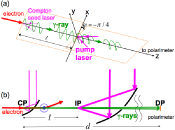
Figure 1: Conceptual experimental setup to investigate the laser-induced vacuum birefringence effect. (a) Definitions of coordinates with respect to the linear polarization plane of the Compton seed laser field and interaction points are provided. (b) Colliding beam geometry with the alignment of the incident electron beam, the parabola mirrors with pinholes and a polarimeter. CP, IP, and DP indicate Compton scattering Point, Interaction Point, and Detection Point, respectively. A distance $l$ between CP and IP and a distance $d$ between CP and DP are introduced. The used electrons are bent in advance of crossing with a pumping laser pulse at IP.

We consider a design of the experiment illustrated in Fig.1 a) for the measurement of the laser-induced birefringence effect. Figure 1 b) shows colliding beam geometry with the alignment of the incident electron beam, the parabola mirrors with pinholes and the polarimeter. The first mirror focuses a weaker laser pulse at CP to generate highly linearly polarized probe $\gamma$-rays via Compton scattering with incident monochromatic electron bunches and then the second mirror focuses an intense laser pulse at IP to pump the vacuum which is synchronized with the weaker laser pulse. The probe $\gamma$-rays penetrate through the pumped domain and the polarization states are altered by the vacuum birefringence effect. Phase retardation embedded within the pumped domain is extracted from the pair-wise topology of the Bethe-Heitler process within the polarimeter at DP. We introduce a distance $l$ between CP and IP and a distance $d$ between CP and DP for later convenience. We must require that the probe $\gamma$-ray energy is not too high in order to avoid the tunneling electron-positron pair production in the intense pump field. We assume 1 GeV probe $\gamma$-rays in the following design. We simultaneously need a high degree of linear polarization for the probe $\gamma$-ray. We note that the reference polarization plane must be parallel to the direction of the polarization of the Compton seed laser ($x-y$ plane in Fig.1 (a)) and the pump laser must be aligned with a relative rotation angle of $\pm\pi/4$ from that reference plane. This configuration produces equal amplitudes for mutually orthogonal electromagnetic field components of probe photons and, hence, maximizes the visibility of phase retardation.

Given a 10 PW-class laser, for instance, what is available at the ELI project with a typical wavelength of 800 nm, we can expect the completely synchronized weak Compton seed and intense pump laser pulses as well as accelerated unpolarized electrons by exploiting the laser-plasma acceleration technique lpa1 ; lpa2 . We will assume that 5 GeV electrons collide with the Compton seed laser pulses head-on. The assumed electron energy is reasonable given the successful demonstration of quasi-monoenergetic electrons at 4.2 GeV acc1 with laser-plasma acceleration. Of course, we may also use accurate 5 GeV electrons from a conventional accelerator as long as the electron source is synchronized with the 10 PW-class laser. Based on this design, we discuss the individual elements from the upper stream in Fig.1 in the following sections.

III Generation of linearly polarized probe $\gamma$-rays

As illustrated in Fig.1, linearly polarized probe $\gamma$-rays can be obtained by the inverse Compton scattering in the forward region of incident electrons interacting with linearly polarized laser pulses in head-on geometry. In order to efficiently get higher energy photons for a given electron energy and keep the spot size of generated $\gamma$-rays as small as possible GammaGamma , we utilize the multi-photon absorption in the nonlinear Compton scattering process. The $\gamma$-ray yields are estimated by using the cross sections of the nonlinear Compton scattering process for the linearly polarized cases parallel($\parallel$) and perpendicular($\perp$) to the linear polarization plane of the seed Compton laser field slac1 . As follows, the differential cross sections for $n$-photon absorption are expressed as a function of $u\equiv(k_{1}k_{2})/(k_{1}p_{2})$ with, respectively, the initial and final state photon four-momenta $k_{1}$ and $k_{2}$ and the final state electron four-momentum $p_{2}$, and of azimuthal angle $\phi$, which is defined as a rotation angle of the linear polarization plane of $k_{2}$ with respect to the incident linear polarization plane of $k_{1}$:

$$\frac{d\sigma_{\parallel}}{dud\phi}=2{r_{0}}^{2}\frac{m^{2}}{s-m^{2}}\frac{1}{\eta^{2}(1+u)^{2}}\times\\ \left[-2A^{2}_{0}\sigma+4\eta^{2}\left(1+\frac{u^{2}}{4(1+u)}\right)(A^{2}_{1}-A_{0}A_{2})\right],$$ (1)

$$\frac{d\sigma_{\perp}}{dud\phi}=2{r_{0}}^{2}\frac{m^{2}}{s-m^{2}}\frac{1}{\eta^{2}(1+u)^{2}}\times\\ \left[-2A^{2}_{0}(1-\sigma)+\eta^{2}\frac{u^{2}}{1+u}(A^{2}_{1}-A_{0}A_{2})\right]$$ (2)

with

$$\sigma\equiv 1+\frac{(u_{n}-u)(\eta^{2}+1)(1-\cos 2\phi)}{2u}$$ (3)

where $A_{l}$($l$=0,1,2) are defined as

$$A_{l}(\alpha_{Lin},\beta_{Lin},n)=\frac{1}{2\pi}\int^{\pi}_{-\pi}d\Phi\times\\ \cos^{(l)}\Phi\exp\{i\alpha_{Lin}\sin\Phi-i\beta_{Lin}\sin 2\Phi-in\Phi\}$$ (4)

with

$$\alpha_{Lin}=-2\sqrt{2}n\frac{\sqrt{u(u_{n}-u)}}{u_{n}}\frac{\eta}{\sqrt{1+\eta^{2}}}\cos\phi$$ (5)

and

$$\beta_{Lin}=\frac{nu}{2u_{n}}\frac{\eta^{2}}{1+\eta^{2}},$$ (6)

where $s\equiv(p_{1}+k_{1})^{2}$ with the incident electron four-momentum $p_{1}$, the electron mass $m$, and $r_{0}=e^{2}/(4\pi m)=\alpha/m=2.82\times 10^{-13}\mbox{cm}$ with the fine structure constant $\alpha=1/137$. These cross sections are characterized by a nonlinearity parameter $\eta\equiv e\sqrt{-\langle A_{\mu}A^{\mu}\rangle}/mc^{2}$ with the four-vector potential of the incident photon $A_{\mu}$ accompanying a variable $u_{n}\equiv 2(k_{1}p_{1})n/(m^{2}(1+\eta^{2}))$ for the $n$-photon absorption case.

We summarize a set of reachable beam parameters for a laser pulse, an electron bunch, and generated $\gamma$-ray probes per laser-electron crossing via nonlinear Compton scattering in Tab.1. The laser power and intensity results in $\eta=0.62$. A similar range of $\eta=0.4$ has been tested by the SLAC experiment slac2 and we expect the cross sections are still valid. Probe photons at GeV energies are generated within a small scattering angle $\vartheta$ measured from the incident electron direction and the dominant photon yield are confined in $\vartheta<1/\gamma_{e}$ rad where $\gamma_{e}$ is the Lorentz factor of the incident electrons. We consider a narrow bandwidth $\gamma$-rays within 1.015 - 1.021 GeV and emission angle less than or equal to 1/(10$\gamma_{e})=1.022\times 10^{-5}$ rad. This energy range corresponds to the case when the number of absorbed laser photons reaches $n=3$. The limitation of the emission angle is actually necessary to select highly polarized $\gamma$-rays and can be required by putting a narrow collimater at a distant point in front of the polarimeter.

Laser wavelength	$\lambda=800$ nm
Laser pulse energy	$E_{L}=2.2$ mJ
The number of laser photons	$N_{L}\equiv\frac{E_{L}}{hc/\lambda}$
Laser pulse duration	$\tau_{L}$ = 33.5 fs
Laser pulse waist	${w_{L}}_{x}={w_{L}}_{y}=1.6$ $\mu$m
Laser pulse power	66.6 GW
Laser pulse intensity	8.28 W/cm2
Electron energy	5 GeV
Electron bunch waist	${w_{e}}_{x}={w_{e}}_{y}=1$ $\mu$m
Electron bunch length	3 $\mu$m
# of electrons	$N_{e}=10^{10}$
# of absorbed laser photons	$n=3$
$\gamma$-ray energy range in $\vartheta<1/(10\gamma_{e})$	$1.015-1.021$ GeV
# of $\gamma$-rays ($\parallel$) in $\vartheta<1/(10\gamma_{e})$	${N_{\gamma}}_{\parallel}=64090$
# of $\gamma$-rays ($\perp$) in $\vartheta<1/(10\gamma_{e})$	${N_{\gamma}}_{\perp}=890$

Table 1: A set of beam parameters for a laser pulse, an electron bunch, and generated $\gamma$-ray probes per laser-electron crossing via nonlinear Compton scattering.

The number of generated probe photons $N_{\gamma}$ per laser-electron crossing can be numerically evaluated as

$$N_{\gamma}=\int^{\tau_{L}}_{0}dt{\cal L}\int^{2\pi}_{0}d\phi\int^{1/(10\gamma_{e})}_{0}d\vartheta\frac{d\sigma_{\parallel/\perp}}{du}\frac{du}{d\vartheta},$$ (7)

where ${\cal L}$ is laser-electron luminosity per crossing in head-on collision geometry which is defined as

$${\cal L}=\frac{1}{\tau_{L}}\frac{N_{e}N_{L}}{2\pi\sqrt{{w_{L}}^{2}_{x}+{w_{e}}^{2}_{x}}\sqrt{{w_{L}}^{2}_{y}+{w_{e}}^{2}_{y}}}.$$ (8)

The partially integrated cross sections are $1.59\times 10^{-20}\mu$m² and $2.21\times 10^{-22}\mu$m² yielding the numbers of generated $\gamma$-rays 64090 and 890 for $\parallel$ and $\perp$ cases, respectively.

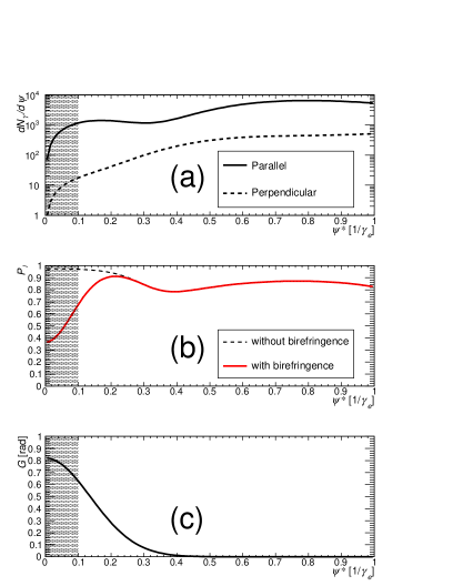
Figure 2: (a) Incident $\gamma$-ray yields as a function of the emission angle for orthogonal linear polarization states, respectively. (b) The degree of linear polarization of $\gamma$-rays. The polarization-flip effect due to the laser-induced birefringence depends on the emission angle. (c) The corresponding phase retardation $G$.

IV Expected phase retardation in the conceptual design

In the quantum mechanical view point, phase retardation may be interpreted as a consequence of polarization flips of probe photons. The degree of linear polarization of probe photons can be defined as

$$P_{l}=\frac{N_{\parallel}-N_{\perp}}{N_{\parallel}+N_{\perp}},$$ (9)

where $N_{\parallel}$ and $N_{\perp}$ are, respectively, the numbers of probe photons with linear polarization states parallel and perpendicular to the direction of the linear polarization of the pump laser. The polarization-flip phenomenon in an intense pump field has been discussed and quantified by Dinu et al. Dinu2014 . In order to parametrize the flipping probability of probe photons with energy $\omega$ for a given pump laser pulse as summarized in Tab.1, we impose following requirements:

• bandwidth is small: $(\Delta\omega_{0}/\omega_{0})^{2}\ll 1$

• validate pulse approximation: $(s^{2}\omega_{0}/(4\Delta\omega_{0}))^{2}\ll 1$

• Heisenberg-Euler limit: $2\omega\omega_{0}/m^{2}\ll 1$,

where $\omega_{0}$ is the pump photon energy, $\Delta\omega_{0}$ satisfies $\tau_{0}=\sqrt{8\log 2}/\Delta\omega_{0}$ with the pump pulse duration $\tau_{0}$, and $s=\lambda_{0}/(\pi w_{0})$ corresponds to the beam divergence with the pump beam waist $w_{0}$ and the pump laser wavelength $\lambda_{0}$. Under these conditions, suppose probe photons collide head-on with a focused pump pulse having a Gaussian profile, as illustrated in Fig.1, the flipping probability of probe photons is approximated as

$$P_{f}=\left(\frac{\alpha}{15}\frac{1}{E_{s}^{2}}\frac{{\cal E}_{0}\omega}{\pi^{2}w_{0}^{2}}\right)^{2}{\rm e}^{-\frac{4\psi^{2}}{\psi_{0}^{2}}}$$

$$\mbox{with}\quad\psi_{0}={\rm tan}^{-1}\frac{w_{0}}{l},$$ (10)

where $\alpha$ is the fine structure constant, $E_{s}$ is the Schwinger critical electric field, $w_{0}$ is the waist size of the focused laser, ${\cal E}_{0}$ is the energy of the pump laser, $\psi$ is the incident angle of probe $\gamma$-rays with respect to the head-on direction and $l$ is the distance between CP and IP in Fig.1 (b). The effect of the incident angle distribution of $\gamma$-rays or misalignment with respect to the head-on collisions is expressed as the exponential reduction of the flipping probability.

A natural experimental observable is thus the reduction of the degree of linear polarization from $P_{l}$ to $(1-2P_{f})P_{l}$. However, in the case of GeV probe photons, there is no known polarizer to directly determine $N_{\parallel}$ and $N_{\perp}$ in experiments. In addition, there could be other sources to reduce $P_{l}$ than the pure phase retardation effect embedded at IP in Fig.1 (b). Dinu et al. Dinu2014 also discuss the relation between the flipping probability and the phase retardation. If we have a way to directly determine the phase retardation itself in a polarimeter, we may be able to discriminate the true birefringent effect from the other sources of reduction of $P_{l}$. In the next section, we will provide the theoretical basis for this idea. We thus provide here the definition of phase retardation $G$ in our notation in accordance with the following section,

$$G\equiv 2\delta\sim\frac{2\sqrt{P_{f}}}{1+\bar{w}}e^{2\rho^{2}\frac{\bar{w}}{1+\bar{w}}}$$ (11)

where $\delta$ is the same definition as in Eq.(36) of Dinu et al.’s paper Dinu2014 as a function of $\rho\equiv r/w_{0}$ with the transverse position $r$ relative to the beam waist $w_{0}$ by introducing the ratio of probe to target beam waists $\bar{w}\equiv 2w^{2}/w^{2}_{0}$.

We now consider the case summarized in Tab.2 where the generated polarized $\gamma$-rays penetrate through the focal region of the pump laser after traveling a distance $l$. Assuming a conservative waist size for the focal spot of $w_{0}=2.4$ ${\rm\mu m}$, a wavelength of 800 nm, a pulse energy of 200 J and an intensity of $3.7\times 10^{22}$ W/cm², the degree of linear polarization of the incident $\gamma$-rays is expected to change from $\langle P_{l}\rangle=0.97$ to $\langle(1-2P_{f})P_{l}\rangle=0.53$ after passing through the laser-induced birefringent vacuum, where $\langle\cdot\cdot\cdot\rangle$ represents the weighted mean of the degree of the polarization over the angular range from $\psi$ = 0 to $\psi$ = $1/(10\gamma_{e})$ and the flipping probability, $P_{f}$, has been calculated with the given laser parameters and $l$ = 10 cm.

Pump laser photon energy	$\omega_{0}=1.55$ eV
Pump laser pulse energy	${\cal E}_{0}=200$ J
Pump laser pulse duration	$\tau_{0}=30$ fs
Pump laser pulse beam diameter	50 cm
Pump laser pulse waist with F#=2.35	$w_{0}=2.4$ $\mu$m
Pump laser pulse intensity	$3.7\times 10^{22}$ W/cm2
Probe $\gamma$-ray energy	$\omega=1$ GeV
Distance $l$	10 cm
Probe $\gamma$-ray waist, $l\tan\{1/(10\gamma_{e})\}$, at IP	$w=1.0$ $\mu$m
Geometrically averaged phase retardation	$\langle G\rangle=0.72$

Table 2: A set of parameters for a single pump laser pulse and linearly polarized 1 GeV probe photons.

Figure 2 (a) shows incident $\gamma$-ray yields as a function of the emission angle with respect to the direction of the incident electron based on Eq.(1), (2), (7) and (8). The horizontal axis $\psi^{*}$ in Fig. 2 is the deduced emission angle, which is normalized to the inverse of the Lorentz factor for 5 GeV electrons. The components parallel and perpendicular to the polarization direction of the Compton seed laser are depicted by solid and dotted lines in Fig.2 (a), respectively. The polarization-flip effect appears as a reduction of the degree of linear polarization, as shown in Fig.2 (b). A large polarization-flip effect is visible in the forward direction, especially for $\psi^{*}<1/10$. Figure 2 (c) shows the corresponding phase retardation $G$. The average of $G$ within $\psi^{*}<1/10$ with $\bar{w}=0.35$ reaches $\langle G\rangle=0.72$ rad.

V Extracting phase retardation from pair-wise topology of the Bethe-Heitler process

Determining of the degree of linear polarization of incident photons via the Bethe-Heitler process is proposed in Ref.pair_pol1 and the method has been applied to several experiments, for example, Ref.pair_pol5 ; pair_pol6 ; pair_pol7 . The detailed theoretical basis can also be found in Ref.pair_pol3 ; pair_pol4 . However, there is no explicit calculation for a general ellipsoidally polarized case to date. Because phase retardation $G$ is close to unity in our case, we cannot approximate the polarization state of $\gamma$-rays penetrating though the pumped domain as the linearly polarized state anymore. In this section we thus derive the pair-wise angular distribution with contemporary notations, e.g., found in Ref.Greiner in order to explicitly implement phase retardation $G$ into polarization vectors of incident photons so that the theoretical functional form is directly applicable to the concrete polarimeter proposed in the next section.

The differential cross section $d\sigma$ is expressed as

$$d\sigma=\int\frac{|S_{fi}|^{2}}{T\frac{v_{in}}{V}}V\frac{d^{3}p_{+}}{(2\pi)^{3}}V\frac{d^{3}p_{-}}{(2\pi)^{3}},$$ (12)

where $S_{fi}$ is the transition amplitude within a time interval $T$ and a normalized volume $V$ of the conversion process from an initial photon state $i$ with relative velocity $v_{in}=c$ to a fixed Coulomb potential of a target nucleus into an electron and positron pair in the final state $f$ whose four-momenta are $p_{-}$ and $p_{+}$, respectively. With respect to the static Coulomb potential with a point charge $-Ze$, the transition amplitude is described as Greiner

$$S_{fi}=Ze^{3}2\pi\delta(E_{+}+E_{-}-\omega)\sqrt{\frac{4\pi}{2\omega V}}\sqrt{\frac{m^{2}}{E_{+}E_{-}V^{2}}}\frac{4\pi}{|q|^{2}}\\ \times\bar{u}(p_{-},s_{-})\left[(-i{\ooalign{\hfil/\hfil\crcr$\epsilon$}})\frac{i}{{\ooalign{\hfil/\hfil\crcr$p_{-}$}}+{\ooalign{\hfil/\hfil\crcr$k$}}-m}(-i\gamma^{0})+\right.\\ \left.(-i\gamma^{0})\frac{i}{-{\ooalign{\hfil/\hfil\crcr$p_{+}$}}+{\ooalign{\hfil/\hfil\crcr$k$}}-m}(-i{\ooalign{\hfil/\hfil\crcr$\epsilon$}})\right]v(p_{+},s_{+})\\ \equiv-iZe^{3}2\pi\delta(E_{+}+E_{-}-\omega)\sqrt{\frac{4\pi}{2\omega V}}\sqrt{\frac{m^{2}}{E_{+}E_{-}V^{2}}}\frac{4\pi}{|q|^{2}}\\ \times\bar{u}(p_{-},s_{-})\Gamma v(p_{+},s_{+})$$ (13)

where electron and positron spinors, $u$ and $v$, respectively, with the equal mass $m$, Dirac matrices $\gamma^{\mu}$ with $\mu=0\sim 3$ giving the Feynman slash notation ${\ooalign{\hfil/\hfil\crcr$A$}}\equiv\gamma^{\mu}A_{\mu}$ for an arbitrary four-dimensional vector $A$, incident photon four-momentum $k\equiv(\omega,\vec{k})$ with the four-dimensional polarization vector $\epsilon$, four-momentum transfer $q\equiv p_{+}+p_{-}-k$ with $p_{+}\equiv(E_{+},\vec{p_{+}})$ and $p_{-}\equiv(E_{-},\vec{p_{-}})$, and $\Gamma$ is defined in Eq.(16). With $\alpha=e^{2}/(\hbar c)\equiv e^{2}$ and, in general, $(2\pi\delta^{2}(E_{f}-E_{i}))^{2}=2\pi\delta(0)2\pi\delta(E_{f}-E_{i})=2\pi T\delta(E_{f}-E_{i})$, we can express the square of the transition amplitude as

$$|S_{fi}|^{2}=Z^{2}e^{6}(2\pi)^{2}\delta^{2}(E_{+}+E_{-}-\omega)\times\\ \left(\frac{4\pi}{2\omega V}\right)\left(\frac{m^{2}}{E_{+}E_{-}V^{2}}\right)\frac{(4\pi)^{2}}{|q|^{4}}\cal{F}\\ =Z^{2}\alpha^{3}2\pi T\delta(E_{+}+E_{-}-\omega)\times\qquad\qquad\\ (4\pi)^{3}\frac{1}{V^{3}}\frac{m^{2}}{2\omega E_{+}E_{-}}\frac{1}{|q|^{4}}\cal{F}$$ (14)

with

$${\cal F}\equiv\left(\bar{u}(p_{-},s_{-})\Gamma v(p_{+},s_{+})\right)\left(\bar{u}(p_{-},s_{-})\Gamma v(p_{+},s_{+})\right)^{\dagger}\\ =\left(\bar{u}(p_{-},s_{-})\Gamma v(p_{+},s_{+})\right)\left(\bar{v}(p_{+},s_{+})\bar{\Gamma}u(p_{-},s_{-})\right)$$ (15)

where

$$\Gamma\equiv{\ooalign{\hfil/\hfil\crcr$\epsilon$}}\frac{{\ooalign{\hfil/\hfil\crcr$p_{-}$}}-{\ooalign{\hfil/\hfil\crcr$k$}}+m}{-2p_{-}\cdot k}\gamma^{0}+\gamma^{0}\frac{-{\ooalign{\hfil/\hfil\crcr$p_{+}$}}+{\ooalign{\hfil/\hfil\crcr$k$}}+m}{-2p_{+}\cdot k}{\ooalign{\hfil/\hfil\crcr$\epsilon$}}$$ (16)

and

$$\bar{\Gamma}\equiv\gamma^{0}\Gamma^{\dagger}\gamma^{0}=\gamma^{0}\frac{{\ooalign{\hfil/\hfil\crcr$p_{-}$}}-{\ooalign{\hfil/\hfil\crcr$k$}}+m}{-2p_{-}\cdot k}{\ooalign{\hfil/\hfil\crcr$\epsilon$}}^{*}+{\ooalign{\hfil/\hfil\crcr$\epsilon$}}^{*}\frac{-{\ooalign{\hfil/\hfil\crcr$p_{+}$}}+{\ooalign{\hfil/\hfil\crcr$k$}}+m}{-2p_{+}\cdot k}\gamma^{0}.$$ (17)

Here we note that $*$ is explicitly displayed only for the polarization vector part including imaginary components as we discuss later. Substituting Eq.(14) into Eq.(12) with $v_{in}=c\equiv 1$, we get

$$d\sigma=\int 8Z^{2}\alpha^{3}\delta(E_{+}+E_{-}-\omega)(2\pi)^{4}\times\\ \frac{m^{2}}{2\omega E_{+}E_{-}}\frac{1}{|q|^{4}}{\cal F}\frac{d^{3}p_{+}d^{3}p_{-}}{(2\pi)^{6}}\\ =\int\frac{4Z^{2}\alpha^{3}m^{2}}{(2\pi)^{2}\omega E_{+}E_{-}}\frac{1}{|q|^{4}}\delta(E_{+}+E_{-}-\omega)d^{3}p_{+}d^{3}p_{-}{\cal F}\qquad\\ =\int dE_{-}\frac{4Z^{2}\alpha^{3}m^{2}}{(2\pi)^{2}\omega E_{+}E_{-}}\frac{1}{|q|^{4}}\delta(E_{+}+E_{-}-\omega)\times\mbox{\hskip 105.2751pt}\\ |\vec{p_{-}}|E_{-}d\Omega_{-}|\vec{p_{+}}|E_{+}dE_{+}d\Omega_{+}{\cal F}\\ =\frac{Z^{2}\alpha^{3}}{(2\pi)^{2}}\frac{4m^{2}}{\omega|q|^{4}}|\vec{p_{-}}||\vec{p_{+}}|dE_{+}d\Omega_{+}d\Omega_{-}\Theta(\omega-E_{+}-m){\cal F}\quad$$ (18)

We then define $F$ by summing ${\cal F}$ over the possible electron and positron spin states as

$$F\equiv\sum_{s_{-},s_{+}}\text{tr}\left[\frac{{\ooalign{\hfil/\hfil\crcr$p_{-}$}}+m}{2m}\Gamma\frac{{\ooalign{\hfil/\hfil\crcr$p_{+}$}}-m}{2m}\bar{\Gamma}\right]\\ \equiv\frac{1}{16m^{2}}\left[\frac{A}{(p_{-}\cdot k)^{2}}+\frac{B}{(p_{-}\cdot k)(p_{+}\cdot k)}+\right.\\ \left.\frac{C}{(p_{+}\cdot k)(p_{-}\cdot k)}+\frac{D}{(p_{+}\cdot k)^{2}}\right]$$ (19)

with

$$A\equiv\text{tr}\left[({\ooalign{\hfil/\hfil\crcr$p_{-}$}}+m){\ooalign{\hfil/\hfil\crcr$\epsilon$}}({\ooalign{\hfil/\hfil\crcr$p_{-}$}}-{\ooalign{\hfil/\hfil\crcr$k$}}+m)\gamma^{0}\right.\\ \left.({\ooalign{\hfil/\hfil\crcr$p_{+}$}}-m)\gamma^{0}({\ooalign{\hfil/\hfil\crcr$p_{-}$}}-{\ooalign{\hfil/\hfil\crcr$k$}}+m){\ooalign{\hfil/\hfil\crcr$\epsilon$}}^{*}\right]\\ B\equiv\text{tr}\left[({\ooalign{\hfil/\hfil\crcr$p_{-}$}}+m){\ooalign{\hfil/\hfil\crcr$\epsilon$}}({\ooalign{\hfil/\hfil\crcr$p_{-}$}}-{\ooalign{\hfil/\hfil\crcr$k$}}+m)\gamma^{0}\qquad\qquad\qquad\qquad\right.\\ \left.({\ooalign{\hfil/\hfil\crcr$p_{+}$}}-m){\ooalign{\hfil/\hfil\crcr$\epsilon$}}^{*}({\ooalign{\hfil/\hfil\crcr$p_{-}$}}-{\ooalign{\hfil/\hfil\crcr$k$}}+m)\gamma^{0}\right]\\ C\equiv\text{tr}\left[({\ooalign{\hfil/\hfil\crcr$p_{-}$}}+m)\gamma^{0}(-{\ooalign{\hfil/\hfil\crcr$p_{+}$}}+{\ooalign{\hfil/\hfil\crcr$k$}}+m){\ooalign{\hfil/\hfil\crcr$\epsilon$}}\qquad\qquad\qquad\quad\right.\\ \left.({\ooalign{\hfil/\hfil\crcr$p_{+}$}}-m)\gamma^{0}({\ooalign{\hfil/\hfil\crcr$p_{-}$}}-{\ooalign{\hfil/\hfil\crcr$k$}}+m){\ooalign{\hfil/\hfil\crcr$\epsilon$}}^{*}\right]\\ D\equiv\text{tr}\left[({\ooalign{\hfil/\hfil\crcr$p_{-}$}}+m)\gamma^{0}(-{\ooalign{\hfil/\hfil\crcr$p_{+}$}}+{\ooalign{\hfil/\hfil\crcr$k$}}+m){\ooalign{\hfil/\hfil\crcr$\epsilon$}}\qquad\qquad\qquad\quad\right.\\ \left.({\ooalign{\hfil/\hfil\crcr$p_{+}$}}-m){\ooalign{\hfil/\hfil\crcr$\epsilon$}}^{*}(-{\ooalign{\hfil/\hfil\crcr$p_{+}$}}+{\ooalign{\hfil/\hfil\crcr$k$}}+m)\gamma^{0}\right]$$ (20)

where we note $F$ has dimension of eV^-2.

Let us remind of the Jones matrix in order to introduce a general ellipsoidally polarized vector beginning from a linearly polarized photon in the $x$-direction. The Jones matrix in $x-y$ coordinate is defined as Yariv

$$W(\varphi,G)=\left(\begin{array}[]{cc}\cos\varphi&\sin\varphi\\ -\sin\varphi&\cos\varphi\\ \end{array}\right)\times$$ (23)

$$\left(\begin{array}[]{cc}e^{-iG/2}&0\\ 0&e^{iG/2}\\ \end{array}\right)\left(\begin{array}[]{cc}\cos\varphi&-\sin\varphi\\ \sin\varphi&\cos\varphi\\ \end{array}\right),$$ (28)

where $\varphi$ denotes a rotation angle of the linear polarization plane of the pump laser field with respect to the linear polarization plane of an incident probe $\gamma$-ray in our case. Following Fig.1 (a) indicating $\varphi=-\pi/4$ with respect to the $x$-axis, the $x-y$ polarization vector after penetrating through the pumped domain is expressed as

$$\left(\begin{array}[]{c}\epsilon_{x}\\ \epsilon_{y}\\ \end{array}\right)=W(-\pi/4,G)\left(\begin{array}[]{c}1\\ 0\\ \end{array}\right)=\left(\begin{array}[]{c}\cos\frac{G}{2}\\ i\sin\frac{G}{2}\\ \end{array}\right).$$ (35)

We then extend this ellipsoidally polarized vector of a probe $\gamma$-ray into a four-dimensional polarization vector as follows

$$\epsilon\equiv\cos\frac{G}{2}g_{1}+i\sin\frac{G}{2}g_{2}$$ (36)

with $g_{1}=(0,1,0,0)$ and $g_{2}=(0,0,1,0)$. In this case the corresponding Feynman slash variables are defined as

$${\ooalign{\hfil/\hfil\crcr$\epsilon$}}=\cos\frac{G}{2}\gamma^{1}+i\sin\frac{G}{2}\gamma^{2}$$ (39)

$${\ooalign{\hfil/\hfil\crcr$\epsilon$}}^{*}=\cos\frac{G}{2}\gamma^{1}-i\sin\frac{G}{2}\gamma^{2}.$$ (42)

By performing the trace calculation in Eq.(19) with $g_{0}=(1,0,0,0)$, $F$ can be expressed with products of four-vectors as follows:

$$F=\frac{1}{16m^{2}}\frac{8}{(k\cdot p_{-})^{2}(k\cdot p_{+})^{2}}\Biggl{[}(k\cdot p_{+})\biggl{\{}(k\cdot p_{-})\\ \times\Bigl{(}(k\cdot p_{+})\bigl{\{}(\cos G+1)(g_{1}\cdot p_{-})^{2}-(\cos G-1)(g_{2}\cdot p_{-})^{2}\\ +2\omega\bigl{(}(g_{0}\cdot p_{-})+(g_{0}\cdot p_{+})\bigr{)}-(k\cdot p_{+})\bigr{\}}-2\omega^{2}(p_{-}\cdot p_{+})-2m^{2}\omega^{2}\Bigr{)}\\ -(k\cdot p_{+})\Bigl{(}2(g_{0}\cdot p_{+})\bigl{(}\omega-(g_{0}\cdot p_{-})\bigr{)}-(k\cdot p_{+})+(p_{-}\cdot p_{+})+m^{2}\Bigr{)}\\ \times\Bigl{(}(\cos G+1)(g_{1}\cdot p_{-})^{2}-(\cos G-1)(g_{2}\cdot p_{-})^{2}\Bigr{)}\\ +2\omega\Bigl{(}(g_{0}\cdot p_{-})+(g_{0}\cdot p_{+})\Bigr{)}(k\cdot p_{-})^{2}-(k\cdot p_{-})^{3}\biggr{\}}\\ +(\cos G+1)(g_{1}\cdot p_{+})^{2}(k\cdot p_{-})^{2}\\ \times\bigl{\{}2(g_{0}\cdot p_{-})\bigl{(}(g_{0}\cdot p_{+})-\omega\bigr{)}+(k\cdot p_{-})+(k\cdot p_{+})-(p_{-}\cdot p_{+})-m^{2}\bigr{\}}\\ +(\cos G-1)(g_{2}\cdot p_{+})^{2}(k\cdot p_{-})^{2}\\ \times\bigl{\{}2(g_{0}\cdot p_{-})\bigl{(}\omega-(g_{0}\cdot p_{+})\bigr{)}-(k\cdot p_{-})-(k\cdot p_{+})+(p_{-}\cdot p_{+})+m^{2}\bigr{\}}\\ +2(\cos G+1)(g_{1}\cdot p_{-})(g_{1}\cdot p_{+})(k\cdot p_{-})(k\cdot p_{+})\\ \times\bigl{\{}(g_{0}\cdot p_{-})\bigl{(}\omega-2(g_{0}\cdot p_{+})\bigr{)}+\omega(g_{0}\cdot p_{+})-(k\cdot p_{-})\\ -(k\cdot p_{+})+(p_{-}\cdot p_{+})+m^{2}-\omega^{2}\bigr{\}}\\ +2(\cos G-1)(g_{2}\cdot p_{-})(g_{2}\cdot p_{+})(k\cdot p_{-})(k\cdot p_{+})\\ \times\bigl{\{}(g_{0}\cdot p_{-})\bigl{(}2(g_{0}\cdot p_{+})-\omega\bigr{)}-\omega(g_{0}\cdot p_{+})+(k\cdot p_{-})\\ +(k\cdot p_{+})-(p_{-}\cdot p_{+})-m^{2}+\omega^{2}\bigr{\}}\Biggr{]}-16.$$ (43)

We used FeynmanCalcFeynmanCalc for the trace calculation. In the proceeding calculations we introduce following definitions of four-momentum with components in Cartesian coordinates and also polar coordinates for $p_{+}$ and $p_{-}$:

$$k\equiv(\omega,0,0,\omega)\\ p_{+}\equiv(E_{+},{p_{+}}_{x},{p_{+}}_{y},{p_{+}}_{z})\mbox{\hskip 128.0374pt}\\ =(E_{+},|\vec{p_{+}}|\sin\theta_{+}\cos\phi_{+},|\vec{p_{+}}|\sin\theta_{+}\sin\phi_{+},|\vec{p_{+}}|\cos\theta_{+})\\ p_{-}\equiv(E_{-},{p_{-}}_{x},{p_{-}}_{y},{p_{-}}_{z})\mbox{\hskip 128.0374pt}\\ =(E_{-},|\vec{p_{-}}|\sin\theta_{-}\cos\phi_{-},|\vec{p_{-}}|\sin\theta_{-}\sin\phi_{-},|\vec{p_{-}}|\cos\theta_{-})\\ q\equiv(p_{+}+p_{-})-k\mbox{\hskip 142.26378pt}\\ =(0,\quad{p_{+}}_{x}+{p_{-}}_{x},\quad{p_{+}}_{y}+{p_{-}}_{y},\quad{p_{+}}_{z}+{p_{-}}_{z}-\omega),$$ (44)

where energy conservation $\omega=E_{+}+E_{-}$ is required for $q$. Because the cross section is maximized in the case of $q\rightarrow 0$, we consider only symmetrically emitted $e^{+}e^{-}$ pairs within the same emission plane with following conditions

$$E_{-} = E_{+}=\omega/2$$ (45)

$$\theta_{-} = \theta_{+}$$

$$\phi_{-} = \phi_{+}+\pi.$$

Fortunately, in this symmetric case, the exact analytical expression for the square of the invariant amplitude can be quite simplified as follows

$$F_{sym}=\frac{1}{16m^{2}}\frac{16\left(\omega^{2}-4m^{2}\right)}{\omega^{2}}\sin^{2}\theta_{+}(\cos G\cos 2\phi_{+}+1).\\$$ (46)

From Eq.(18) with $|\vec{p_{-}}|=|\vec{p_{+}}|=\sqrt{\frac{\omega^{2}}{4}-m^{2}}$ and $dE_{+}=\frac{1}{2}d\omega$, $d\theta_{+}=d\theta_{-}$ and $d\phi_{+}=d\phi_{-}$, the differential cross section in terms of positron-relevant variables for the symmetric case is expressed as

$$\frac{d\sigma_{sym}}{d\omega d\phi_{+}d\theta_{+}}=\int_{0}^{2\pi}d\phi_{-}\delta(\phi_{-}-(\phi_{+}+\pi))\int_{0}^{\pi}d\theta_{-}\delta(\theta_{-}-\theta_{+})\\ \times\frac{1}{2}\frac{Z^{2}\alpha^{3}}{(2\pi)^{2}}\frac{4m^{2}}{\omega|\vec{q}|^{4}}|\vec{p_{+}}|\sin\theta_{+}|\vec{p_{-}}|\sin\theta_{-}F\Theta(\omega/2-m)\\ =\frac{1}{2}\frac{Z^{2}\alpha^{3}}{(2\pi)^{2}}\frac{4m^{2}}{\omega|\vec{q}_{sym}|^{4}}p^{2}_{+}\sin^{2}\theta_{+}F_{sym}\Theta(\omega/2-m)\mbox{\hskip 42.67912pt}\\ =\frac{Z^{2}(2\alpha)^{3}}{(2\pi)^{2}\omega^{3}}\left(\frac{p_{+}\sin\theta_{+}}{|\vec{q}_{sym}|}\right)^{4}(\cos G\cos 2\phi_{+}+1)\Theta(\omega/2-m),$$ (47)

with $|\vec{q}_{sym}|^{4}\equiv\{2|\vec{p_{+}}|\cos\theta_{+}-\omega\}^{4}$ via the relation $|\vec{q}|^{2}=-q^{2}=\{(|\vec{p_{+}}|\cos\theta_{+}+|\vec{p_{-}}|\cos\theta_{-})-\omega\}^{2}$.

We then express the partially integrated cross section within an experimental coverage $0\leq\theta_{+}\leq\Delta\theta$ and $0\leq\phi<2\pi$ in a measurement. This quantity gives us the conversion efficiency into useful symmetric pairs for the determination of phase retardation $G$. We thus further integrate over $d\phi_{+}$, $d\theta_{+}$ and $d\omega$, which gives

$$\sigma_{sym}\sim\frac{4Z^{2}\alpha}{\pi}\left(\frac{\alpha}{m}\right)^{2}\int^{\langle\omega\rangle+\Delta\omega}_{\langle\omega\rangle-\Delta\omega}d\omega\int_{0}^{\Delta\theta}d\theta_{+}\times\\ \frac{m^{2}(\omega^{2}/4-m^{2})^{2}\sin^{4}\theta_{+}}{\omega^{3}(2\sqrt{\omega^{2}/4-m^{2}}\cos\theta_{+}-\omega)^{4}}\Theta(\omega/2-m)\\ \equiv\frac{4Z^{2}\alpha}{\pi}\sigma_{e}H(\langle\omega\rangle,\Delta\omega,\Delta\theta)\mbox{\hskip 76.82234pt}$$ (48)

with $\sigma_{e}\equiv(\alpha/m)^{2}=(2.8\times 10^{-13}\text{cm})^{2}=0.0784~{}\text{b}$.

For $\langle\omega\rangle=1$ GeV, $\Delta\omega/\langle\omega\rangle=0.005$ and $\Delta\theta=0.01$, $H(\langle\omega\rangle,\Delta\omega,\Delta\theta)=0.239$ is obtained. If we choose $Z=79$ (a gold converter), the cross section reaches $\sigma_{sym}=1.1$ b, even if we require the special symmetric case of pair-wise topology in experiments.

VI Polarimetry

VI.1 Parametrization for pair-wise angular distributions

The degree of linear polarization of the $\gamma$-rays is characterized by the anisotropic angular distribution of emission planes containing electron-positron pairs with respect to the polarization plane of the incident $\gamma$-rays  pair_pol1 ; pair_pol3 ; pair_pol4 ; pair_pol5 ; pair_pol6 ; pair_pol7 . At the same time energies of $\gamma$-rays above 100 MeV can be reconstructed by the kinematical relations for the conversion process from a $\gamma$-ray into an electron-positron pair. If offline selections in experiments allow us to impose the symmetric condition in Eq.(45), we can parametrize the angular distribution based on the expression in Eq.(47) by taking other bias factors into account. One of the biases would be initially caused by the degree of linear polarization of probe $\gamma$-rays, because we have to accept a finite angular spread of incident $\gamma$-rays as indicated in Fig.2 (a). Even if we limit the angular spread in $\psi^{*}<0.1$, the averaged degree of linear polarization is 97 %. In such a case, by denoting $\phi$ as the angle of the $e^{+}e^{-}$ emission plane with respect to the linear polarization plane of the Compton seed laser for the case $G=0$, linearly polarized photons in $\parallel$ and $\perp$ directions cause an uncorrelated statistical ensemble of $P\cos 2\phi$ and $Q\cos(2(\phi+\pi/2))$ with the different statistical weights $P=N_{\parallel}/(N_{\parallel}+N_{\perp})$ and $Q=N_{\perp}/(N_{\parallel}+N_{\perp})$ resulting in $P_{l}\cos(2\phi)$ with $P_{l}=P-Q$ as defined in Eq.(9). In addition to this known bias, in general, experimental resolutions would reduce the amplitude of the modulation. By taking these factors into account, the angular distribution of emission planes containing individual $e^{+}e^{-}$ pairs can be parametrized as follows

$$\frac{dN_{e^{+}e^{-}}}{d\phi}=N_{0}\left(1+AP_{l}\cos G\cos(2\phi-\phi_{0})\right),$$ (49)

where $N_{0}$ is the number of $e^{+}e^{-}$ pairs in the unpolarized case and $\phi_{0}$ is an offset phase. The analyzing power, $A$, refers to the reduction of anisotropy caused by experimental resolution. The offset phase is introduced to allow the offset angle of the polarimeter plane ($x-z$ plane in Fig.3) with respect to the linear polarization plane of the Compton seed laser  ($x-z$ plane in Fig.1 (a)). In the proceeding discussion, we always assume $\phi_{0}=0$.

VI.2 Polarimeter design

There are two key issues in the design of the $\gamma$-ray polarimeter. The first is how to deal with a large number of $\gamma$-rays confined within a cone angle of $1/(10\gamma_{e})$. In our estimation summarized in Tab.1, $\sim 6.5\times 10^{4}$ $\gamma$-rays at 1 GeV are expected to enter into a detector at a time. For this purpose, the $\gamma$-ray converter must be carefully chosen in order to adjust the number of $e^{-}e^{+}$ pairs depending on the handling capability of the polarimeter. To accurately spot the 1/(10$\gamma_{e})\sim 10^{-5}$ rad, we need to locate the converter far from the interaction point. If the converter is located at $d=10$ m in Fig.1 (b), the angular spread results in the transverse spread of 100 $\mu$m on the converter. This suggests that a conventional silicon pixel type sensor with a few 10 $\mu$m resolution is useful for this type of polarimetry.

The second issue is how to accurately reconstruct an emission plane based on the momentum vectors of an $e^{-}e^{+}$ pair produced at the conversion point, which has the greatest effect on the analyzing power in the end. The opening angle of a pair at the conversion point is the key information needed to correctly reconstruct the anisotropy in Eq.(49). The original angle is, however, smeared by multiple Coulomb scatterings during passage through the conversion material. In addition, multiple Coulomb scatterings inside each pixel sensor also give rise to a displacement of the measured hits from the ideal trajectory of a charged particle. This displacement degrades the track finding and reconstructing capabilities and reduces the analyzing power. Thus, the thickness of the detector materials must be controlled to keep the analyzing power at an acceptable level.

The minimum elements of the detector design are illustrated in Fig.3. The detection system simultaneously performs spectroscopy and polarimetry for a multiple $\gamma$-ray injection. It is composed of a converter at the front followed by a narrow collimator to guarantee the narrow angular spread, that is, narrow energy band of the incident probe $\gamma$-rays, a static magnetic field, and three-layers of pixel sensors. The converter is chosen to suppress the smearing effect due to multiple Coulomb scatterings but to keep the pair creation efficiency reasonably high. These two requirements are in a trade-off relation as a function of the thickness and the atomic number of the conversion material. We assume a gold foil with a thickness of 2 $\mu$m resulting in a conversion efficiency of $1.3\times 10^{-5}$ based on the partially integrated cross section of the symmetric Bethe-Heitler process as discussed in Eq.(48). Given the parameters in Tab.1, the expected number of conversion pairs per shot is 0.84, which is close to unity.

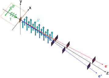
Figure 3: Configuration of the detection elements for $\gamma$-ray polarimetry and spectroscopy via the Bethe-Heitler process on a thin converter located at the origin.

VI.3 Capability to extract phase retardation

The feasibility of extracting phase retardation with the detector configuration illustrated in Fig.3 was evaluated using the Geant4 simulation toolkitgeant1 ; geant2 . In the following evaluation, for simplicity, we assume a total number of conversion pairs as $10^{4}$ with a single pair production per shot, which is likely achievable in high-intensity laser facilities such as ELI eli , where 10 PW laser pulses are available with one shot per minute resulting in 9 days in order to exceed $10^{4}$ pairs with the expectation value of 0.84 pairs per shot. A static magnetic field of 0.6 T over 12 cm was assumed just behind the converter which is enough to measure the sub-GeV momenta of the charge-separated electrons and positrons. To provide this field, a permanent-magnet-based dipole would be preferable from the point of view of the compactness and homogeneity of the field in order to allow us to arbitrarily rotate the magnet system together with the set of sensors around the $z$-axis. The three-layered position sensors made of silicon pixels are located downstream of the magnet system with the total length of the polarimeter of 25 cm from the converter. The pixel size and the thickness of the pixel sensor were assumed to be 20 $\mu$m and 50 $\mu$m, respectively.

As a result of the simulation, we found that the $\gamma$-ray energy can be reconstructed from the measured momenta of an $e^{-}e^{+}$ pair with an energy resolution of 7.8$\%$ at $\omega=1$ GeV. This energy resolution is sufficient to select a narrow enough energy range to guarantee the high degree of linear polarization of incident 1.0 GeV $\gamma$-rays based on the offline selection of pairs, because multi-photon absorption $n=2$ and $n=4$ cases give energies 0.726-0.730 GeV and 1.268-1.275 GeV in $\psi*<0.1$, respectively, which can be discriminated from the $n=3$ case 1.015-1.021 GeV with the 7.8% resolution.

Figure 4 shows reconstructed angular distributions of pair emission planes with respect to the reference plane ($\phi_{0}=0$). We assume the creation of a single $e^{-}e^{+}$ pair per shot via the conversion process with a total pair statistics of $10^{4}$ in this simulation.

The open blue and closed red points depict the angular distributions for $G=0$ and $0.72$, respectively. The raw amplitudes of the angular distributions fit with Eq.(49) are obtained as $A(0.72)P_{l}\cos(0.72)=0.529\pm 0.013$ and $A(0)P_{l}\cos(0)=0.665\pm 0.011$ where the errors include statistical errors and also biases from the effect of the finite sensor segment and the track reconstruction algorithm. The analyzing power $A$ has a monotonic $G$ dependence and we can evaluate them as A(0.72) = 0.725 and A(0) = 0.686 from the simulation in advance.

The reduction of the raw amplitude in $G=0.72$ from that of the null phase retardation case, 0.136, can reach a high enough significance level compared to the error size of the null retardation case, 0.011. Therefore, we can declare the observation of phase retardation via vacuum birefringence given the statistics of $10^{4}$ pairs by this method.

The averaged phase retardation $\langle G\rangle$ can then be extracted from $\langle G\rangle=\cos^{-1}\left(P_{l}\cos(0.72)/P_{l}\cos(0)\right)=0.720\pm 0.034$ with the same statistics after correcting the analyzing power biases at the different $G$ values. We note that experiments do not necessarily have to quantify $P_{l}$ precisely because $P_{l}$ should be common to $G=0$ and $G=0.72$ cases and systematically canceled out. From this simulation result, we evaluate that the accuracy of the reconstructed $\langle G\rangle$ can reach 4.7%.

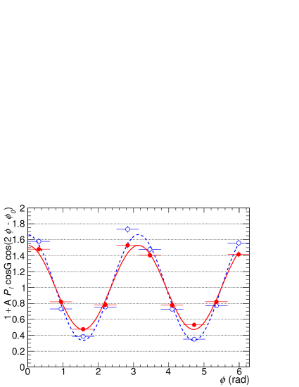
Figure 4: The angular distributions of $e^{-}e^{+}$ emission planes with respect the reference plane ($\phi_{0}=0$). The open blue and closed red points depict the angular distributions for $G=0$ and $0.72$, respectively, with fitting results based on Eq.(49). The total number of $e^{-}e^{+}$ pairs was assumed to be $10^{4}$ with a single pair production per shot in this simulation. The vertical error bars show statistical errors in the simulation.

VI.4 Possible sources of depolarization

We consider several background sources which possibly change the degree of linear polarization of probe $\gamma$-rays before entering into the gold converter of the polarimeter with $d=1000$ cm in Fig.1.

The dominant background source would come from the mixture of two linear polarization states in the nonlinear Compton scattering process. How to correct the effect of $P_{l}$ of probe photons has been already discussed in the previous subsection.

The remaining contributions are from possible interactions characterized by individual cross sections $\sigma_{\gamma A}$ between $\gamma$-rays and residual atoms $A$ in the vacuum system along the distance $d$. The number of interacting $\gamma$-rays is approximated as $N_{int}\sim\sigma_{\gamma A}n_{A}d$ with number density of residual atoms $n_{A}$. A typical vacuum system maintained at $\sim 10^{-5}$ Pa results in $n_{A}\sim 10^{10}\mbox{cm}^{-3}$ compared to $n_{A}\sim 10^{20}\mbox{cm}^{-3}$ in the atmospheric pressure. The possible interactions between GeV probe photons and atoms are pair creations, Compton scattering, and Delbrück scattering Delbrueck . The first two processes eventually absorb probe photons or change the probe photon energy drastically, hence, they can be no serious background for the phase retardation measurement as long as the narrow energy range and limited conversion points on the converter of the polarimeter are imposed in the measurement. The interaction resulting in non-absorbed photons with the same energy as the generated energy at the Compton scattering vertex is thus limited to forward Delbrück scattering via $\gamma+A\rightarrow\gamma+A$.

The differential forward Delbrück scattering cross section per solid angle for high energy photons close to GeV is expected to be described as $d\sigma_{\gamma A}/d\Omega={\cal A}^{2}(\alpha Z)^{4}(r_{0})^{2}\sim{\cal A}^{2}(\alpha Z)^{4}0.1$ b with the classical electron radius $r_{0}$ FowawrdDelbrueck . The scattering amplitude is evaluated as ${\cal A}\sim 10^{3}$ at maximum for 1 GeV FowawrdDelbrueck . Even for Kr($Z=54$), corresponding highest $Z$ in the air, $d\sigma_{\gamma A}/d\Omega\sim(10^{3})^{2}(54/137)^{4}0.1\sim 10^{3}$ b at most. For the assumed $d$ and $n_{A}$, we expect $N_{int}\sim 10^{-21}[\mbox{cm}^{2}]10^{10}[\mbox{cm}^{-3}]10^{3}[\mbox{cm}]=10^{-8}$ per shot, which is negligible with respect to $6.5\times 10^{4}$ probe photons per shot for the polarization measurement. Furthermore, by taking following facts into account: i) the proper abundance of Kr as well as the same effects from the other residual atoms with lower $Z$ in the air, ii) no reason to expect that residual atoms are polarized with respect to the incident polarization plane of probe photons over the entire length $d$, and iii) very narrow solid angle in front of the polarimeter, we expect that the depolarization effect by Delbrück scattering is totally negligible.

The robustness to the background contributions is one of advantages to use GeV probe photons compared to, for example, the case of the PVLAS experiment where careful controls of the vacuum pressure are required because eV photons more often interact with residual atoms and the atoms could be weakly polarized by the external static magnetic field along the entire path of probe photons. We note, however, that tests of birefringence with different probe wavelengths are essentially important in order to complete the measurement of the dispersion relation in the laser-induced vacuum.

VII Conclusion and prospects

We have considered combining a 10 PW laser system with 1 GeV linearly polarized probe $\gamma$-rays to enhance the sensitivity to the measurement of the laser-induced birefringence effect. We have derived formulae to directly determine phase retardation close to unity from pair-wise topology of the symmetric Bethe-Heitler process. We conclude that if $10^{4}$ pairs are available, it is possible to observe the vacuum birefringence effect with the accuracy of 4.7% for $\langle G\rangle=0.72$. This result is based on a realistic set of laser parameters and potentially realizable statistics for 10 PW systems such as ELI projects eli .

Given the firm theoretical and experimental footing in the simplest QED case, the proposed approach with the compact polarimeter design would open up a new arena of fundamental physics to explore more dynamical and complicated vacuum states realized in laboratories, astrophysical objects and possibly the early Universe.

- (1) I. T. Drummond, S. J. Hathrell, Phys. Rev. D22 343 (1980).
- (2) J.S. Toll, The Dispersion Relation for Light and its Application to Problems Involving Electron Pairs, Ph.D thesis, Princeton University, 1952 (unpublished)
- (3) K. Scharnhorst, Phys. Lett. B 236 354 (1990).
- (4) G. M. Shore, Nucl. Phys. B 778, 219 (2007)
- (5) J. Magueijo, Rept. Prog. Phys. 66 2025 (2003); S. H. S. Alexander and J. Magueijo, hep-th/0104093.
- (6) W. Dittrich and H. Gies, Probing the Quantum Vacuum, Springer, Berlin (2007).
- (7) A. Di Piazza, C. Müller, K. Z. Hatsagortsyan, and C. H. Keitel, Rev. Mod. Phys. 84, 1177 (2012).
- (8) V. Dinu, T. Heinzl, A. Ilderton, M. Marklund and G. Torgrimsson, Phys. Rev. D 89, 125003 (2014).
- (9) http://www.eli-laser.eu/
- (10) C. Thompson and R. C. Duncan, Mon. Not. Roy. Astron. Soc. 275 (1995) 255; ibid. Astrophys. J. 473 (1996) 322.
- (11) A. Adare et al., Phys. Rev. Lett. 104, 132301 (2010).
- (12) D. E. Kharzeev, L. D. McLerran, and H. J. Warringa, Nucl. Phys. A 803, 227-253 (2008).
- (13) S. Ozaki, T. Arai, K. Hattori, and K. Itakura, Phys. Rev. D 92, 016002 (2015).
- (14) F. D. Valle et al., Phys. Rev. D 90, 092003 (2014).
- (15) A. Cadene et al., Eur. Phys. J. D 68, 16 (2014).
- (16) R. Cameron et al., Phys. Rev. D 47, 3707 (1993).
- (17) K. Homma, D. Habs and T. Tajima, Appl. Phys. B 104, 769 (2011).
- (18) T. Heinzl, B. Liesfeld, K. U. Amthor, H. Schwoerer, R. Sauerbrey and A. Wipf, Opt. Commun. 267, 318 (2006)
- (19) F. Karbstein and C. Sundqvist, Phys. Rev. D 94, no. 1, 013004 (2016)
- (20) B. Marx, I. Uschmann, S. Hofer, R. Lotzsch, O. Werhrhan, E. Förster, M. Kaluza, T. Stöhlker, H. Gies, C. Detlefs, T. Roth, J. Härtwig, G.G. Paulus, Opt. Commun. 284, 915 (2011).
- (21) V. Dinu, T. Heinzl, A. Ilderton, M. Marklund and G. Torgrimsson, Phys. Rev. D 90, 045025 (2014).
- (22) G. Cantatore, F. Della Valle, E. Milotti, L. Dabrowski and C. Rizzo, Phys. Lett. B 265, 418 (1991).
- (23) T. N. Wistisen and U. I. Uggerhj, Phys. Rev. D 88, no. 5, 053009 (2013).
- (24) T. Tajima and J. M. Dawson, Phys. Rev. Lett. 43, 267(1979).
- (25) C. Joshi et al., Nature 311, 525 (1984).
- (26) W. P. Leemans et al., Phys. Rev. Lett. 113, 245002(2014).
- (27) K. Homma, K. Matsuura and K. Nakajima, PTEP 2016, no. 1, 013C01 (2016).
- (28) K. D. Shmakov, Study of nonlinear QED effects in interactions of terawatt laser with high-energy electron beam, Ph.D thesis, University of Tennessee, 1997, SLAC-R-666, UMI-98-23127, UMI-98-23127-MC.
- (29) C. Bamber et al., Phys. Rev. D 60, 092004 (1999).
- (30) T. H. Berlin and L. Madansky, Phys. Rev.78, 623 (1950).
- (31) C. N. Yang. Phys. Rev. 77, 722 (1950).
- (32) B. Wojtsekhowskia, D. Tedeschib and B. Vlahovicc, Nucl. Instr. Meth. A515, 605 (2003).
- (33) C. de Jager et al., Eur. Phys. J. A 19, Supplement 1, 275 (2004).
- (34) D. Bernard, Nucl. Instr. Meth. A729, 765-780 (2013).
- (35) H. Olsen and L.C. Maximon, Phys. Rev. 114, 887 (1959).
- (36) L.C. Maximon and H. Olsen, Phys. Rev. 126, 887 (1962).
- (37) W. Greiner and J. Reinhardt, QUANTUM ELECTRODYNAMICS Second Edition, Springer (1994).
- (38) A. Yariv, Optical Electronics in Modern Communications (Oxford University Press, Inc. 1997).
- (39) R. Mertig, Comput. Phys. Comm., 60:165, 1991.
- (40) S. Agostinelli et al., Nucl. Instr. and Meth. A 506, 250 (2003).
- (41) J. Allison et al., IEEE Trans. Nucl. Sci. 53, 270 (2006).
- (42) M. Delbrück, Z. Physik 84, 144 (1933).
- (43) F. Rohrlich and R. L. Gluckstern, Phys. Rev. 86, 1 (1952).