Central-limit approach to risk-aware Markov decision processes

Abstract

Whereas classical Markov decision processes maximize the expected reward, we consider minimizing the risk. We propose to evaluate the risk associated to a given policy over a long-enough time horizon with the help of a central limit theorem. The proposed approach works whether the transition probabilities are known or not. We also provide a gradient-based policy improvement algorithm that converges to a local optimum of the risk objective.

1 Introduction

Markov Decision Processes (MDPs) are essential models for stochastic sequential decision-making problems (e.g., Puterman, 2014; Bertsekas, 1995; Sutton and Barto, 1998). Classical MDPs are concerned with the expected performance criteria. However, in many practical problems, risk-neutral objectives may not be appropriate (cf. Ruszczyński, 2010, Example 1).

Risk-aware decision-making is prevalent in the financial mathematics and optimization literature (e.g., Artzner et al., 2002; Rockafellar, 2007; Markowitz et al., 2000; Von Neumann and Morgenstern, 2007), but limited to single-stage decisions. Risk-awareness has been adopted in multi-stage or sequential decision problems more recently. A chance-constrained formulation for MDPs with uncertain parameters has been discussed in (Delage and Mannor, 2010). A criteria of maximizing the probability of achieving a pre-determined target performance has been analyzed in (Xu and Mannor, 2011). In (Ruszczyński, 2010), Markov risk measure is introduced and a corresponding risk-averse policy iteration method is developed. A mean-variance optimization problem for MDPs is addressed in (Mannor and Tsitsiklis, 2013). A generalization of percentile optimization with objectives defined by a measure over percentiles instead of a single percentile is introduced in (Chen and Bowling, 2012). In terms of computational convenience, actor-critic algorithms for optimizing variance-related risk measures in both discounted and average reward MDPs have been proposed in (Prashanth and Ghavamzadeh, 2013). Mean and conditional value-at-risk optimization problem in MDPs is solved by policy gradient and actor-critic algorithms in (Chow and Ghavamzadeh, 2014). A unified policy gradient approach is proposed in (Tamar et al., 2015) to seek optimal strategy in MDPs with the whole class of coherent risk measures. Risk-aversion in multiarmed bandit problems is studied in (Yu and Nikolova, 2013), where algorithms are proposed with PAC guarantees for best arm identification. Robust MDPs (e.g., Nilim and El Ghaoui, 2005; Iyengar, 2005) mitigate the sensitivity of optimal policy to ambiguity in the underlying transition probabilities, and are closely related to the risk-sensitive MDPs. Such relations are uncovered by Osogami (2012).

In this work, we study the value-at-risk in finite-horizon MDPs. Computing this risk associated with a sequence of decision using the defintion and first principles is intractable. However, we show that this computation is made tractable by using a central limit theorem for Markov chains (Jones et al., 2004; Kontoyiannis and Meyn, 2003; Glynn and Meyn, 1996). For a long-enough horizon $T$ and a fixed policy $\pi$, we are thus able to evaluate the risk associated with following policy $\pi$ over $T$ time steps. Specifically, our first contributions are policy evaluation algorithms whether the transition probability matrix induced by $\pi$ is known or not. Under mild conditions, we provide high-probability error bounds for the evaluation.

For a fixed risk measure $\rho$, and a space of policies that is parametrized by $\theta$, our second contribution is a policy improvement algorithm that converges in finite iterations, under certain assumptions, to a locally optimal policy. This approach updates the parameter $\theta$ in the direction of gradient of the risk measure. Compared to the previous work, our proposed method does not explicitly approximate the value function. Therefore, it does not have approximation error due to the selection of value function approximator.

Even though we deal mainly with the static value-at-risk risk measure (defined by the cumulative reward), our results can be easily extended to deal with the conditional- or average-value-at-risk by using its definition Schied (2004).

1.1 Distinction from related works

It is important to note that our risk measure is very different from the dynamic risk measure analyzed in (Ruszczyński, 2010), which has the following recursive structure: for $T$-length horizon MDP and policy $\pi$, the dynamic risk measure $\rho_{T}$ is defined as

$$r(x_{0}^{\pi})+\gamma\rho\left(r(x_{1}^{\pi})+\gamma\rho\Big{(}r(x_{2}^{\pi})+\gamma\rho\big{(}\ldots+r(x_{T}^{\pi})\big{)}\Big{)}\right),$$

where $r$ is a state dependent reward function, $\gamma<1$ is a constant and $\rho$ is a Markov risk measure, i.e., the evaluation of each static coherent risk measure $\rho$ is not allowed to depend on the whole past. In contrast, our risk measure emphasizes the statistical properties of the reward accumulated over multiple time steps: it is similar to that used in (Yu and Nikolova, 2013) in the context of bandit problems.

From the computational and algorithmic perspective, we evaluate the policy and obtain the risk value directly. Different from the work (Prashanth and Ghavamzadeh, 2013; Chow and Ghavamzadeh, 2014; Tamar et al., 2015), which indirectly evaluated the risk value by using function approximation, our proposed method has an explicit policy evaluation step and does not require value function approximation. Therefore, it does not have approximation error due to the selection of value function approximator and the richness of the features. Moreover, for risk-aware MDPs that are known to be NP-hard (e.g., Delage and Mannor, 2010; Xu and Mannor, 2011), our method can find approximated solutions to those problems.

From the conceptual perspective, our work is the first attempt to consider general risk measures with a central-limit approach. Compared with (Tamar et al., 2015), our approach is not limited to so-called “coherent” risk measures (both static and dynamic), whose defining properties are not satisfied by the value-at-risk. The methods proposed in (Tamar et al., 2015) thus cannot be applied. Moreover, the time horizon in our setup is allowed to be infinite. Other previous work (Delage and Mannor, 2010; Xu and Mannor, 2011; Mannor and Tsitsiklis, 2013) restrict themselves to specific risk criteria: Delage and Mannor (2010) considered a set of percentile criteria; Xu and Mannor (2011) seek to find the policy that maximizes the probability of achieving a pre-determined target performance, and Mannor and Tsitsiklis (2013) discussed a mean-variance optimization problem.

This paper is organized as follows: In Section 2 we provide background and problem statement. For a fixed policy, we then evaluate its risk value in Section 3. In specific, we discuss the policy evaluation algorithms in Section 3.1 and 3.2 when the transition kernel is either known or unknown. The main result is Theorem 2, which bounds the error of true and estimated asymptotic variances. In Section 4, we provide policy gradient algorithm to improve the fixed policy. A conclusion is offered in Section 5.

2 Problem formulation

MDP is a tuple $\langle\mathcal{X},\mathcal{A},P,r,T\rangle$, where $\mathcal{X}$ is a finite set of states, $\mathcal{A}$ is a finite set of actions, $P$ is the transition kernel, $T$ is the (possibly infinite) moderate time horizon, and $r(x,a):\mathcal{X}\times\mathcal{A}\rightarrow\mathbb{R}$ is the bounded and measurable reward function. A function $F:\mathcal{X}\rightarrow\mathbb{R}$ is called lattice if there are $h>0$ and $0\leq d<h$, such that $\frac{F(x)-d}{h}$ is an integer for $x\in\mathcal{X}$. The minimal $h$ for such condition holds is called the span of $F$. If the function $F$ can be written as a sum $F=F_{0}+F_{l}$, where $F_{l}$ is lattice with span $h$ and $F_{0}$ has zero asymptotic variance (which will be defined later), then $F$ is called almost-lattice. Otherwise, $F$ is called strongly nonlattice. We assume the functional $r$ is strongly nonlattice. A policy $\pi$ is the rule according to which actions are selected at each state. We parameterize the stochastic policies by $\{\pi(\cdot|x;\theta),x\in\mathcal{X},\theta\in\Theta\subseteq\mathbb{R}^{k_{1}}\}$, and denote the set of policies by $\Pi$. Since in this setting a policy $\pi$ is represented by its $k_{1}$-dimensional parameter vector $\theta$, policy dependent functions can be written as a function of $\theta$ in place of $\pi$. So, we use $\pi$ and $\theta$ interchangeably in the paper.

Given a policy $\pi\in\Pi$, a Markov reward process $X^{\pi}=\{x_{t}^{\pi}:x\in\mathcal{X},t\in T\}$ is induced by $\pi$. We write the transition kernel of the induced Markov process and dependent rewards as $P^{\pi}$ and $r(x^{\pi}_{t})$ for all $t\in T$, respectively. We denote $(P^{\pi})^{n}$ as the $n$-step Markov transition kernel corresponding to $P^{\pi}$. We are interested in the long-term behavior of the sum

$$S_{T}^{\pi}=\sum_{t=0}^{T-1}r(x_{t}^{\pi}),\quad T\geq 1.$$

If the Markov chain is positive recurrent with invariant probability measure $\xi^{\pi}$, we define the mean of reward function $r$ as

$$\varphi^{\pi}(r)=\lim_{T\rightarrow\infty}\frac{1}{T}\mathbb{E}\left[\sum_{t=0}^{T-1}r(x_{t}^{\pi})\right],$$ (1)

where $x_{0}^{\pi}$ is the initial condition and $\mathbb{E}$ is the expectation over the Markov process $X^{\pi}$. Equivalently, the mean can be expressed as

$$\varphi^{\pi}(r)=\sum_{x}\xi^{\pi}(x)r(x).$$ (2)

Often we can quantify the rate of convergence of (1) by showing that the limit

$$\hat{r}^{\pi}(x)=\lim_{T\rightarrow\infty}\mathbb{E}\left[\sum_{t=0}^{T-1}r(x_{t}^{\pi})-T\varphi^{\pi}(r)\right]$$

exists where, in fact, the function $\hat{r}^{\pi}(x)$ solves the Poisson equation

$$P^{\pi}\hat{r}^{\pi}=\hat{r}^{\pi}-r+\varphi^{\pi}(r)\mathbf{1}.$$ (3)

Here $P^{\pi}$ operates on functions $\hat{r}^{\pi}:\mathcal{X}\rightarrow\mathbb{R}$ via $P^{\pi}\hat{r}^{\pi}(x)=\sum_{y}P(x,y)\hat{r}^{\pi}(y)$, $r$ is the vector form of $r(x)$ and $\mathbf{1}$ is the vector with all elements being $1$.

Let $\mathcal{Y}$ denote the set of bounded random variables, and let $\rho:\mathcal{Y}\rightarrow\mathbb{R}$ denote a risk measure. Our risk-aware objective is

$$\min_{\pi\in\Pi}\quad\rho\left(S_{T}^{\pi}\right).$$ (4)

We discuss specific types of risk measures in the coming sections. All proofs are deferred in the supplementary material due to space constraints.

3 Policy evaluation

In this section, we develop methods to evaluate the risk value $\rho(S^{\pi}_{T})$ for a fixed policy $\pi$. In specific, we consider the Markov chain $X^{\pi}$ induced by policy $\pi$, which is assumed to be geometrically ergodic. We then apply limit theorems for geometrically ergodic Markov chain in (Kontoyiannis and Meyn, 2003) to obtain the distribution function of cumulative reward when transition kernel is either known or unknown. Finally, we provide algorithms for computing some examples of risk measures.

Similar to Kontoyiannis and Meyn (2003), we make the following two standard assumptions for the Markov process $X^{\pi}$.

Assumption 1.

The Markov process $X^{\pi}$ is geometrically ergodic with Lyapunov function $V$ (i.e., $\psi-$irreducible, aperiodic and satisfying Condition (V4) of Kontoyiannis and Meyn (2003)) where $V:\mathcal{X}\rightarrow[1,\infty)$ satisfies $\varphi^{\pi}(V^{2})<\infty$.

The detailed definition of geometric ergodicity can be found in (Kontoyiannis and Meyn, 2003, Section 2).

Assumption 2.

The (measurable) reward function $r:\mathcal{X}\rightarrow[-1,1]$ has nontrivial asymptotic variance $\sigma^{2}\triangleq\lim_{t\rightarrow\infty}var_{x}(S^{\pi}_{t}/\sqrt{t})>0$.

Under Assumption 1 and 2, Kontoyiannis and Meyn (2003) showed that the following result holds.

Theorem 1 (Theorem 5.1, Kontoyiannis and Meyn (2003)).

Suppose that $X^{\pi}$ and the strongly nonlattice functional $r$ satisfy Assumption 1 and 2, and let $G^{\pi}_{T}(y)$ denote the distribution function of the normalized partial sums $\frac{S^{\pi}_{T}-T\varphi^{\pi}(r)}{\sigma\sqrt{T}}$:

$$G^{\pi}_{T}(y)\triangleq\mathbb{P}\left\{\frac{S^{\pi}_{T}-T\varphi^{\pi}(r)}{\sigma\sqrt{T}}\leq y\right\}.$$

Then, for all $x^{\pi}_{0}\in\mathcal{X}$ and as $T\rightarrow\infty$,

$$G^{\pi}_{T}(y)=g(y)+\frac{\gamma(y)}{\sigma\sqrt{T}}\left[\frac{\varrho}{6\sigma^{2}}(1-y^{2})-\hat{r}^{\pi}(x^{\pi}_{0})\right]+o(T^{-\frac{1}{2}}),$$

uniformly in $y\in\mathbb{R}$, where $\gamma(y)$ denotes the standard normal density and $g(y)$ is the corresponding distribution function. Here $\varrho$ is a constant related to the third moment of $S_{T}^{\pi}/\sqrt{T}$. The definitions of $\varrho$ and term $o(T^{-1/2})$ can be found in the supplementary material.

Unlike (Heyman and Sobel, 2003), which considered finite Markov chains and obtained the moments of the cumulative reward, we further impose geometric ergodicity assumption on the Markov process $X^{\pi}$. By doing this, we are able to utilize the explicit form of distribution function given by (Kontoyiannis and Meyn, 2003, Theorem 5.1) with the time error term $o(T^{-1/2})$. In addition, the geometric ergodicity property enables us to bound the approximation error in Theorem 2.

Similar to Glynn and Meyn (1996), we define the fundamental kernel $Z^{\pi}$ associated with fixed $\pi$ as

$$Z^{\pi}=(H^{\pi})^{-1},$$

where the kernel $\Xi^{\pi}$ is defined as $\Xi^{\pi}(x,\cdot)=\xi^{\pi}(\cdot)$, and $H^{\pi}\triangleq I-P^{\pi}-\Xi^{\pi}$. If the inverse of $H^{\pi}$ is well defined, Glynn and Meyn (1996) stated that the solution to Poisson equation (3) has the form

$$\hat{r}^{\pi}=Z^{\pi}(r-\varphi^{\pi}(r)\mathbf{1}).$$ (5)

When $\sigma^{2}<\infty$ and $\varphi^{\pi}(\hat{r}^{\pi})<\infty$, Meyn and Tweedie (2012, Equation 17.44) showed that the asymptotic variance $\sigma^{2}$ can be obtained by

$$\sigma^{2} =\lim_{n\rightarrow\infty}\frac{\mathbb{E}[(S^{\pi}_{n}-n\varphi^{\pi}(r))^{2}]}{n}=\sum_{x\in\mathcal{X}}[\hat{r}^{\pi}(x)^{2}-(P^{\pi}\hat{r}^{\pi}(x))^{2}]\xi^{\pi}(x).$$ (6)

We remark that the asymptotic variance can also be calculated without the knowledge of $\hat{r}^{\pi}$ by Theorem 17.5.3 of Meyn and Tweedie (2012):

$$\sigma^{2}=\sum_{x^{\pi}_{0}\in\mathcal{X}}{\overline{r}_{0}}^{2}\xi^{\pi}(x^{\pi}_{0})+2\sum_{k=1}^{\infty}\sum_{x^{\pi}_{0}\in\mathcal{X}}\overline{r}_{0}\xi^{\pi}(x^{\pi}_{0})\times\sum_{x^{\pi}_{k}\in\mathcal{X}}\overline{r}_{k}P^{\pi}(x,x^{\pi}_{k}|x=x^{\pi}_{0})^{k},$$

where $\overline{r}_{k}=r(x^{\pi}_{k})-\varphi^{\pi}(r)$ and $P^{\pi}(x,y|x=x_{0})^{n}$ denotes the $n$-step transition probability to state $y$ conditioned on the initial state $x_{0}$. It is clear that solving (6) requires the knowledge of transition kernel $P^{\pi}$. In the following subsections, we study the policy evaluation with and without knowing $P^{\pi}$, respectively.

3.1 Transition probability kernel $P^{\pi}$ is known

In this subsection, we propose an algorithm to obtain the distribution function $G_{T}^{\pi}$ in Theorem 1, using which we can evaluate the risk value.

Since transition kernel $P^{\pi}$ is known, we first calculate the stationary distribution $\xi^{\pi}$. Note that the stationary distribution satisfies

$$P^{\pi}\xi^{\pi}=\xi^{\pi}.$$

Thus, the stationary distribution is the eigenvector of matrix $P^{\pi}$ with eigenvalue $1$ (recall that $1$ is always an eigenvalues for matrix $P^{\pi}$), which is unique up to constant multiples under Assumption 1.

After we compute the stationary distribution $\xi^{\pi}$, it is straightforward to calculate the mean (2), solve Poisson equation (3) and get the asymptotic variance (6). Therefore, we are able to obtain the distribution function $G_{T}^{\pi}(y)$ defined in Theorem 1 at this stage. Finally, the risk measures that can be expressed as a function of $G_{T}^{\pi}(y)$ can be evaluated. We provide two examples below.

Example 3.1 ($T$-step value-at-risk).

Let $\lambda$ be given and fixed. The $T$-step value-at-risk is defined by

$$\rho_{\lambda}(S^{\pi}_{T})=VaR_{\lambda}(S_{T}^{\pi})=-q(\lambda),$$

where $q$ is the right-continuous quantile function of $S_{T}^{\pi}$.

When $T$ is moderate, $o(T^{-1/2})$ vanishes, the distribution function $G^{\pi}_{T}(y)$ defined in Theorem 1 has the form

$$G^{\pi}_{T}(y)\approx g(y)+\frac{\gamma(y)}{\sigma\sqrt{T}}\left[\frac{\varrho}{6\sigma^{2}}(1-y^{2})-\hat{r}^{\pi}(x^{\pi}_{0})\right].$$ (7)

This allows us to compute the $T$-step value-at-risk. The procedure is summarized in Algorithm 1. The next example considers the mean-variance risk measure.

Example 3.2 (Mean-variance risk).

Given $\lambda$, the mean-variance risk measure is given by

$$\rho_{\lambda}(S^{\pi}_{T})=-\mu(S^{\pi}_{T})+\lambda\sigma^{2}(S^{\pi}_{T}/\sqrt{T}),$$

where $\mu(S^{\pi}_{T})$ is the mean of $S^{\pi}_{T}$, and $\sigma^{2}(S^{\pi}_{T}/\sqrt{T})$ is the variance of $S^{\pi}_{T}/\sqrt{T}$.

The corollary below gives formula to obtain the mean-variance risk. An algorithm can be obtained similarly for the mean-variance risk simply by replacing line $7$ in Algorithm 1 by the corresponding risk measure. The same procedure can easily be generalized to other risk measures.

Corollary 1.

Under Assumption 1 and 2, given $\lambda$, the mean-variance risk measure can be computed by

$$\rho_{\lambda}(S^{\pi}_{T})=-\varphi(r)+\lambda\sigma^{2}.$$

where $\varphi(r)$ and $\sigma^{2}$ are defined in (2) and (6), respectively.

Algorithm 1 Policy evaluation for $T$-step value-at-risk ($P^{\pi}$ is known)

1:Input: Transition probability matrix $P^{\pi}$ induced by policy $\pi$, initial state $x^{\pi}_{0}$, decision horizon $T\in\mathbb{N}_{+}$, reward function $r$, and the coefficient $\lambda$ of value-at-risk.

2:Obtain stationary distribution $\xi^{\pi}$ by solving the equation $P^{\pi}\xi^{\pi}=\xi^{\pi}$.

3:Substitute $\xi^{\pi}$ in (2) for mean $\varphi^{\pi}(r)=\sum_{x}\xi^{\pi}(x)r(x)$.

4:Solve the Poisson equation (3) for $\hat{r}^{\pi}$ by (5).

5:Compute asymptotic variance in (6): $\sigma^{2}=\sum_{x\in\mathcal{X}}[\hat{r}^{\pi}(x)^{2}-(P^{\pi}\hat{r}^{\pi}(x))^{2}]\xi^{\pi}(x)$.

6:Calculate the constant $\varrho$.

7:Output: The $T$-step value-at-risk, which can be computed by

$$\widetilde{VaR}_{\lambda}(S_{T}^{\pi})=-\inf\left\{y\in\mathbb{R}:G^{\pi}_{T}(h(y))>\lambda\right\},$$

where $G^{\pi}_{T}(y)$ is defined in (7), and $h(y)=\frac{y-T\varphi^{\pi}(r)}{\sigma\sqrt{T}}$.

3.2 Transition probability kernel $P^{\pi}$ needs to be estimated

In practice, knowing transition kernel $P^{\pi}$ is generally hard. In this subsection, we present a policy evaluation algorithm when transition kernel needs to be estimated, and provide the corresponding approximation error.

Intuitively, if the estimated transition kernel is accurate enough, the gap between solutions to estimated and true Poisson equations is small (as shown in Lemma 5), which implies the difference between estimated and true asymptotic variances is also small (as shown in Theorem 2).

A way of estimating transition kernel is to use the empirical distribution. Denoting the required number of samples by $n_{1}$ and the estimated transition kernel by $P_{n_{1}}^{\pi}$, we make the following assumption.

Assumption 3.

There exist $\epsilon_{1}(n_{1})>0$ and $\delta_{1}(n_{1})>0$ such that $\epsilon_{1}(n_{1})\rightarrow 0$ and $\delta_{1}(n_{1})\rightarrow 0$ as $n_{1}\rightarrow\infty$. Moreover, we have the following bound for the error:

$$\mathbb{P}\left(||P^{\pi}_{n_{1}}-P^{\pi}||_{\infty}\leq\epsilon_{1}(n_{1})\right)\geq 1-\delta_{1}(n_{1}).$$

Here the supreme norm $||\cdot||_{\infty}$ of a matrix $A$ is defined as the maximum absolute row sum of the matrix:

$$||A||_{\infty}\triangleq\max_{1\leq i\leq m}\sum_{j=1}^{n}|a_{ij}|.$$

We remark Assumption 3 can be easily satisfied if a large collection of observed data is provided. This could be achievable if one is allowed to simulate the system arbitrarily many times.

Next, we perturb the true transition kernel $P^{\pi}$, define the resulting perturbed transition kernel as $\tilde{P}^{\pi}$ and denote the stationary distribution associated with $\tilde{P}^{\pi}$ as $\tilde{\xi}^{\pi}$. Given $\tilde{P}^{\pi}$, we let $\xi^{\pi}_{n}(\cdot)=\tilde{P}^{\pi}(x,\cdot)^{n}$ be an estimator of $\tilde{\xi}^{\pi}(\cdot)$. Under Assumption 1, we make the following assumption which establishes the convergence of $||\xi^{\pi}_{n}-\tilde{\xi}^{\pi}||$, where $||\cdot||$ is the total variation norm defined as following: If $\mu$ is a signed measure on $\mathcal{B}(\mathcal{X})$, then the total variation norm is defined as

$$||\mu||=\sup_{|f|\leq 1}|\mu(f)|=\sup_{A\in\mathcal{B}(\mathcal{X})}\mu(A)-\inf_{A\in\mathcal{B}(\mathcal{X})}\mu(A).$$

Assumption 4.

Given $\epsilon>0$ and perturbed transition kernel $\tilde{P}^{\pi}\in P$. If $||\tilde{P}^{\pi}-P^{\pi}||_{\infty}\leq\epsilon,$ then for every $n\in\mathbb{N}_{+}$, the geometrically ergodic Markov chain has a form of convergence

$$||\tilde{P}^{\pi}(x,\cdot)^{n}-\tilde{\xi}^{\pi}(\cdot)||\leq M(x)\tau^{n},$$

where $\tau<1$, and $M(x)$ is a nonnegative function.

This assumption essentially guarantees the geometric ergodicity property remains if the original Markov chain is slightly perturbed.

Assumption 3 and 4 immediately imply that

$$\mathbb{P}\left(||P_{n_{1}}^{\pi}(x,\cdot)^{n}-\tilde{\xi}^{\pi}(\cdot)||\leq M(x)\tau^{n}\right)\geq 1-\delta_{1}(n_{1}),$$ (8)

where $\tilde{\xi}^{\pi}$ is the stationary distribution associated with $P^{\pi}_{n_{1}}$. Let $\tau_{1}(P^{\pi})$ be the ergodicity coefficient of transition kernel $P^{\pi}$ (Seneta, 1988), which is defined by

$$\tau_{1}(P^{\pi})=\sup_{\begin{subarray}{c}||\nu||_{1}=1\\ \nu^{\top}\mathbf{e}=0\end{subarray}}||\nu^{\top}P^{\pi}||_{1}.$$ (9)

If the ergodicity coefficient satisfies $0\leq\tau_{1}(P^{\pi})<1$, Cho and Meyer (2001, Equation 3.4) shows

$$||\tilde{\xi}^{\pi}-\xi^{\pi}||_{1}\leq\frac{||P^{\pi}_{n_{1}}-P^{\pi}||_{\infty}}{1-\tau_{1}(P^{\pi})}.$$

Therefore, under Assumption 3, we have

$$\mathbb{P}\left(||\tilde{\xi}^{\pi}-\xi^{\pi}||_{1}\leq\frac{\epsilon_{1}(n_{1})}{1-\tau_{1}(P^{\pi})}\right)\geq 1-\delta_{1}(n_{1}).$$ (10)

The ergodicity coefficient $\tau_{1}(P_{n_{1}}^{\pi})$ for the estimated transition kernel $P_{n_{1}}^{\pi}$ is defined in a same manner.

Matrix $H^{\pi}$ plays an important role in defining solution to Poisson equation. We impose a requirement on the smallest singular value $\sigma_{min}(H^{\pi})$ of $H^{\pi}$.

Assumption 5.

There exists a constant $c>\widetilde{\varpi}(x)$ such that the smallest singular value of matrix $H^{\pi}$ satisfies $\sigma_{min}(H^{\pi})\geq c$. Here

$$\widetilde{\varpi}(x) =\sqrt{|\mathcal{X}|}\left(\epsilon_{1}(n_{1})+\frac{\epsilon_{1}(n_{1})}{1-\tau_{1}(P^{\pi}_{n_{1}})-\epsilon_{1}(n_{1})}+2M(x)\tau^{n_{2}}\right).$$ (11)

Similar to (3), we define the estimated Poisson equation as

$$P^{\pi}_{n_{1}}\hat{r}_{n_{1},n_{2}}^{\pi}=\hat{r}_{n_{1},n_{2}}^{\pi}-r+\varphi_{n_{2}}^{\pi}(r)\mathbf{1},$$ (12)

where $\varphi_{n_{2}}^{\pi}(r)$ is the estimated mean

$$\varphi_{n_{2}}^{\pi}(r)=\sum_{x}\xi^{\pi}_{n_{2}}(x)r(x),$$ (13)

with $\xi^{\pi}_{n_{2}}$ being the estimation of stationary distribution $\tilde{\xi}^{\pi}$

$$\xi^{\pi}_{n_{2}}(\cdot)=P_{n_{1}}^{\pi}(x,\cdot)^{n_{2}}.$$ (14)

We then define the perturbed fundamental kernel as

$$Z_{n_{1},n_{2}}^{\pi}=(H_{n_{1},n_{2}}^{\pi})^{-1},$$

where $H_{n_{1},n_{2}}^{\pi}=I-P_{n_{1}}^{\pi}-\Xi_{n_{2}}^{\pi}$ with $\Xi_{n_{2}}^{\pi}(x,\cdot)=\xi_{n_{2}}^{\pi}(\cdot)$. The following lemma shows $Z_{n_{1},n_{2}}^{\pi}$ is well defined under Assumption 5.

Lemma 1.

Under Assumption 5, $Z_{n_{1},n_{2}}^{\pi}$ is well defined.

The solution to estimated Poisson equation (12) can be expressed as

$$\hat{r}_{n_{1},n_{2}}^{\pi}=Z_{n_{1},n_{2}}^{\pi}(r-\varphi_{n_{2}}^{\pi}(r)\mathbf{1}),$$ (15)

We define the asymptotic variance associated with $\hat{r}_{n_{1},n_{2}}$ as $\sigma_{n_{1},n_{2}}^{2}$, which can be obtained by the equation below:

$$\sigma_{n_{1},n_{2}}^{2}=\sum_{x\in\mathcal{X}}[\hat{r}_{n_{1},n_{2}}^{\pi}(x)^{2}-(P_{n_{1}}^{\pi}\hat{r}_{n_{1},n_{2}}^{\pi}(x))^{2}]\xi_{n_{2}}^{\pi}(x).$$ (16)

The theorem below provides the condition for $n_{2}$ such that the difference between estimated and true asymptotic variances $\sigma^{2}$ and $\sigma_{n_{1},n_{2}}^{2}$ defined in (6) and (16) is small. We provide an outline of the proof below and a complete version can be found in the supplementary material.

Theorem 2.

Given policy $\pi$, $\epsilon\geq 0$, $\lambda\in(0,1)$ and let $\sigma_{n_{1},n_{2}}^{2}$ and $\sigma^{2}$ be the estimated and true asymptotic variances, respectively. Under Assumption 1, 2, 3, 4 and 5, there exists $n_{2}$ such that the following two conditions (C1) and (C2) are satisfied

(C1) $$\frac{|\mathcal{X}|(|\mathcal{X}|+1)^{3}(\widetilde{\varpi}-\sqrt{|\mathcal{X}|}\epsilon_{1}(n_{1}))}{(c-\widetilde{\varpi})^{2}}\leq\lambda\epsilon$$

(C2) $$\frac{\alpha_{2}(x)|\mathcal{X}|}{c}\left(\frac{(|\mathcal{X}|+1)\widetilde{\varpi}}{c-\widetilde{\varpi}}+\sqrt{|\mathcal{X}|}\left(\widetilde{\varpi}-\epsilon_{1}(n_{1})\sqrt{|\mathcal{X}|}\right)\right)+\max_{x\in\mathcal{X}}\alpha_{1}(x)\alpha_{2}(x)|\mathcal{X}|\leq(1-\lambda)\epsilon,$$

where

$$\alpha_{1}(x)= \frac{\epsilon_{1}(n_{1})\sqrt{|\mathcal{X}|}(|\mathcal{X}|+1)}{c-\widetilde{\varpi}}+\frac{|\mathcal{X}|^{\frac{3}{2}}}{c}\left(\frac{\widetilde{\varpi}(|\mathcal{X}|+1)}{c-\widetilde{\varpi}}+\sqrt{|\mathcal{X}|}\left(\widetilde{\varpi}-\epsilon_{1}(n_{1})\sqrt{|\mathcal{X}|}\right)\right),$$

$$\alpha_{2}(x)= \dfrac{|\mathcal{X}|(|\mathcal{X}|+1)(2c-\widetilde{\varpi})}{c(c-\widetilde{\varpi})}.$$

Moreover, we have

$$\mathbb{P}(|\sigma_{n_{1},n_{2}}^{2}-\sigma^{2}|\leq\epsilon)\geq 1-38\delta_{1}(n_{1}).$$

Proof.

By equations (6) and (16), we have

$$|\sigma_{n_{1},n_{2}}^{2}-\sigma^{2}|$$

$$= \bigg{|}\sum_{x\in\mathcal{X}}[{\hat{r}_{n_{1},n_{2}}^{\pi}}(x)^{2}-(P_{n_{1}}^{\pi}\hat{r}_{n_{1},n_{2}}^{\pi}(x))^{2}]\xi^{\pi}_{n_{2}}(x)-\sum_{x\in\mathcal{X}}[{\hat{r}^{\pi}}(x)^{2}-(P^{\pi}\hat{r}^{\pi}(x))^{2}]\xi^{\pi}(x)\bigg{|}$$

$$\stackrel{{\scriptstyle(1)}}{{=}} \bigg{|}\sum_{x\in\mathcal{X}}[{\hat{r}_{n_{1},n_{2}}^{\pi}}(x)^{2}-(P_{n_{1}}^{\pi}\hat{r}_{n_{1},n_{2}}^{\pi}(x))^{2}]\xi^{\pi}_{n_{2}}(x)-\sum_{x\in\mathcal{X}}[{\hat{r}_{n_{1},n_{2}}^{\pi}}(x)^{2}-(P_{n_{1}}^{\pi}\hat{r}_{n_{1},n_{2}}^{\pi}(x))^{2}]\xi^{\pi}(x)$$

$$+\sum_{x\in\mathcal{X}}[{\hat{r}_{n_{1},n_{2}}^{\pi}}(x)^{2}-(P_{n_{1}}^{\pi}\hat{r}_{n_{1},n_{2}}^{\pi}(x))^{2}]\xi^{\pi}(x)-\sum_{x\in\mathcal{X}}[{\hat{r}^{\pi}}(x)^{2}-(P^{\pi}\hat{r}^{\pi}(x))^{2}]\xi^{\pi}(x)\bigg{|}$$

$$\stackrel{{\scriptstyle(2)}}{{\leq}}a_{n}+b_{n},$$

where

$$a_{n}= \bigg{|}\sum_{x\in\mathcal{X}}[{\hat{r}_{n_{1},n_{2}}^{\pi}}(x)^{2}-(P_{n_{1}}^{\pi}\hat{r}_{n_{1},n_{2}}^{\pi}(x))^{2}](\xi^{\pi}_{n_{2}}(x)-\xi^{\pi}(x))\bigg{|},$$

$$b_{n}= \bigg{|}\sum_{x\in\mathcal{X}}[{\hat{r}_{n_{1},n_{2}}^{\pi}}(x)^{2}-(P_{n_{1}}^{\pi}\hat{r}_{n_{1},n_{2}}^{\pi}(x))^{2}]\xi^{\pi}(x)-\sum_{x\in\mathcal{X}}[{\hat{r}^{\pi}}(x)^{2}-(P^{\pi}\hat{r}^{\pi}(x))^{2}]\xi^{\pi}(x)\bigg{|}.$$

Equality $(1)$ holds due to subtracting and then adding a same term $\sum_{x\in\mathcal{X}}[{\hat{r}_{n_{1},n_{2}}^{\pi}}(x)^{2}-(P_{n_{1}}^{\pi}\hat{r}_{n_{1},n_{2}}^{\pi}(x))^{2}]\xi^{\pi}(x)$. Inequality $(2)$ holds by triangle inequality. In order to bound the terms $a_{n}$ and $b_{n}$, we need following lemmas.

First, we derive a bound for $|\tau_{1}(P_{n_{1}}^{\pi})-\tau_{1}(P^{\pi})|$ by the lemma below.

Lemma 2.

Under Assumption 3, the ergodicity coefficient for the estimated transition kernel $P_{n_{1}}^{\pi}$ satisfies

$$\mathbb{P}\left(|\tau_{1}(P_{n_{1}}^{\pi})-\tau_{1}(P^{\pi})|\leq\epsilon_{1}(n_{1})\right)\geq 1-\delta_{1}(n_{1}).$$

Denoting $||a||_{2}$ as the Euclidean norm of vector $a$, we present a lemma showing that the solution (5) of Poisson equation (3) is bounded.

Lemma 3.

Under Assumption 2 and 5, the solution to Poisson equation $\hat{r}^{\pi}$ is bounded $||\hat{r}^{\pi}||_{2}\leq\frac{\sqrt{|\mathcal{X}|}(|\mathcal{X}|+1)}{c}$.

Analogously to Lemma 3, we have the following result.

Lemma 4.

Under Assumption 1, 2, 3, 4 and 5, the solution (15) to estimated Poisson equation (12) is bounded such that

$$\mathbb{P}\left(||\hat{r}_{n_{1},n_{2}}^{\pi}||_{2}\leq\frac{\sqrt{|\mathcal{X}|}(|\mathcal{X}|+1)}{c-\widetilde{\varpi}}\right)\geq 1-4\delta_{1}(n_{1}).$$

The lemma below shows that solutions to the true and estimated Poisson equations are close to each other with high probability.

Lemma 5.

Under Assumption 1, 2, 3, 4 and 5, the difference between solutions to true and estimated Poisson equation is bounded such that

$$\mathbb{P}\left(||\hat{r}^{\pi}-\hat{r}_{n_{1},n_{2}}^{\pi}||_{2}\leq\tilde{\varsigma}\right)\geq 1-7\delta_{1}(n_{1}),$$

where $\tilde{\varsigma}=\frac{\sqrt{|\mathcal{X}|}(|\mathcal{X}|+1)\widetilde{\varpi}}{c(c-\widetilde{\varpi})}+\frac{|\mathcal{X}|}{c}\left(\widetilde{\varpi}-\epsilon_{1}(n_{1})\sqrt{|\mathcal{X}|}\right)$.

Recall that for two random variables $a_{n}$ and $b_{n}$, and $\epsilon\in\mathbb{R}$ with $\lambda\in(0,1)$, by union bound and monotonicity property of probability, we have

$$\mathbb{P}(a_{n}+b_{n}\leq\epsilon)\geq\mathbb{P}(a_{n}\leq\lambda\epsilon)+\mathbb{P}(b_{n}\leq(1-\lambda)\epsilon).$$

Finally, by bounding terms $a_{n}$ and $b_{n}$, we prove the theorem. ∎

Now we are able to compute the $T$-step value-at-risk, which is summarized as a procedure in the Algorithm 2. Note that given the asymptotic variance $\sigma_{n_{1},n_{2}}$ and solution to estimated Poisson equation $\hat{r}_{n_{1},n_{2}}$, when $T$ is moderate, $o(T^{-1/2})$ vanishes, $G^{\pi}_{T}(y)$ defined in Theorem 1 becomes

$$G^{\pi}_{T}(y)\approx g(y)+\frac{\gamma(y)}{\sigma_{n_{1},n_{2}}\sqrt{T}}\left[\frac{\tilde{\varrho}}{6\sigma_{n_{1},n_{2}}^{2}}(1-y^{2})-\hat{r}_{n_{1},n_{2}}^{\pi}(x^{\pi}_{0})\right],$$ (17)

where $\tilde{\varrho}$ is defined in a same manner as $\varrho$ by replacing $P^{\pi}$ and $\xi^{\pi}$ by $P^{\pi}_{n_{1}}$ and $\xi^{\pi}_{n_{2}}$, respectively.

In the following, we analysis the mean-variance risk defined in Example 3.2. Corollary 2 gives formula to obtain the mean-variance risk and provides high-probability bound for the risk measure. An algorithm can be developed for the mean-variance risk simply by replacing line $9$ in Algorithm 2 by the corresponding risk measure.

Corollary 2.

Under Assumption 1, 2, 3, 4 and 5, given $\lambda$, the estimated mean-variance risk measure can be computed by

$$\tilde{\rho}_{\lambda}(S^{\pi}_{T})=-\varphi_{n_{2}}^{\pi}(r)+\lambda\sigma_{n_{1},n_{2}}^{2}.$$

where $\varphi_{n_{2}}^{\pi}(r)$ and $\sigma_{n_{1},n_{2}}^{2}$ are defined in (13) and (16), respectively. Moreover, we have

$$\mathbb{P}\left(|\tilde{\rho}_{\lambda}(S^{\pi}_{T})-\rho_{\lambda}(S^{\pi}_{T})|\leq\kappa\right)\geq 1-41\delta_{1}(n_{1}),$$

where $\rho_{\lambda}(S^{\pi}_{T})$ is the true mean-variance risk value computed in Corollary 1 and $\kappa=2M(x)\tau^{n_{2}}+\frac{\epsilon_{1}(n_{1})}{1-\tau_{1}(P_{n_{1}}^{\pi})-\epsilon_{1}(n_{1})}+\lambda\epsilon$.

A similar argument can be developed for $T$-step value-at-risk defined in Example 3.1. When $\varrho=1$, $\hat{r}=0.5$, $T=100$, $\varphi(r)=0.1$, we plot the distribution functions $G_{T}$ for $\sigma=1$ and $1.1$ below.

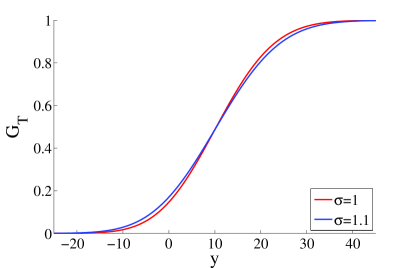
Figure 1: Distribution functions $G_{T}$ for $\sigma=1$ and $1.1$.

Figure 1 shows the distribution functions are close, which implies the corresponding $T$-step value-at-risks are also close to each other (When $\lambda=0.3$, the $T$-step value-at-risks are $5.134$ and $4.632$, respectively).

Algorithm 2 Policy evaluation for $T$-step value-at-risk ($P^{\pi}$ is unknown)

1:Input: Policy $\pi$, initial state $x^{\pi}_{0}$, reward function $r$, decision horizon $T\in\mathbb{N}_{+}$, $\lambda\in(0,1)$ and estimation parameters $\epsilon_{1}(n_{1})$ and $\delta_{1}(n_{1})$.

2:Obtain the estimated transition kernel $P^{\pi}_{n_{1}}$ satisfying Assumption 3 with parameter $\epsilon_{1}(n_{1})$ and $\delta_{1}(n_{1})$.

3:Compute the ergodicity coefficient $\tau_{1}(P^{\pi}_{n_{1}})$ for the estimated transition kernel $P^{\pi}_{n_{1}}$.

4:Choose $n_{2}$ with $\tau_{1}(P^{\pi}_{n_{1}})$ obtained from step $3$ such that conditions in Theorem 2 hold.

5:Compute the estimated stationary distribution $\xi_{n_{2}}^{\pi}$ defined by (14).

6:Calculate the solution of estimated Poisson equation $\hat{r}_{n_{1},n_{2}}^{\pi}$ by (15).

7:Obtain the asymptotic variance $\sigma_{n_{1},n_{2}}^{2}$ defined in (16).

8:Calculate the constant $\tilde{\varrho}$.

9:Output: The $T$-step value-at-risk, which can be computed by

$$\widetilde{VaR}_{\lambda}(S_{T}^{\pi})=-\inf\left\{y\in\mathbb{R}:G^{\pi}_{T}(h(y))>\lambda\right\},$$

where $G^{\pi}_{T}(y)$ is defined in (17), and $h(y)=\frac{y-T\varphi_{n_{2}}^{\pi}(r)}{\sigma_{n_{1},n_{2}}\sqrt{T}}$ with $\varphi_{n_{2}}^{\pi}(r)$ defined in (13).

4 Policy Improvement

In this section, we propose policy gradient methods to improve policy $\pi$ and solve the optimization problem (4). Specifically, we compute the gradient of the performance (i.e., the risk) w.r.t. the policy parameters from the evaluated policies, and improve $\pi$ by adjusting its parameters in the direction of the gradient.

In the following, we make a standard assumption in gradient-based MDPs literature (e.g., Sutton et al., 1999; Konda and Tsitsiklis, 1999; Bhatnagar et al., 2009; Prashanth and Ghavamzadeh, 2013).

Assumption 6.

For any state-action pair $(x,a)$, $\pi(a|x;\theta)$ is continuously differentiable in the parameter $\theta$.

In a recent work, Prashanth and Ghavamzadeh (2013, Section 4) presented actor-critic algorithms for optimizing the risk-sensitive measure that are based on two simultaneous perturbation methods: simultaneous perturbation stochastic approximation (SPSA) (Spall, 1992) and smoothed functional (SF) (Bhatnagar et al., 2012). We use similar arguments here and further apply those methods to estimate the gradient of the risk measure with respect to the policy parameter $\theta$, i.e., $\nabla_{\theta}\rho(S_{T}^{\theta})$.

The idea in these methods is to estimate the gradient $\nabla_{\theta}\rho(S_{T}^{\theta})$ using two simulated trajectories of the system corresponding to policies with parameters $\theta$ and $\theta^{+}=\theta+\beta\triangle$. Here $\beta>0$ is a positive constant and $\triangle$ is a perturbation random variable, i.e., a $k_{1}$-vector of independent Rademacher (for SPSA) and Gaussian $\mathcal{N}(0,1)$ (for SF) random variables.

SPSA-based estimate for $\nabla_{\theta}\rho(S_{T}^{\theta})$ is given by

$$\partial_{\theta^{(i)}}\rho(S_{T}^{\theta})\approx\frac{\rho(S_{T}^{\theta+\beta\triangle})-\rho(S_{T}^{\theta})}{\beta\triangle^{(i)}},\quad i=1,\dots,k_{1}$$ (18)

where $\triangle$ is a vector of independent Rademacher random variables and $\triangle^{(i)}$ is its $i$-th entry. The advantage of this estimator is that it perturbs all directions at the same time (the numerator is identical in all $k_{1}$ components). So, the number of function measurements needed for this estimator is always two, independent of the dimension $k_{1}$.

SF-based estimate for $\nabla_{\theta}\rho(S_{T}^{\theta})$ is given by

$$\partial_{\theta^{(i)}}\rho(S_{T}^{\theta})\approx\frac{\triangle^{(i)}}{\beta}\left(\rho(S_{T}^{\theta+\beta\triangle})-\rho(S_{T}^{\theta})\right),i=1,\dots,k_{1}$$ (19)

where $\triangle$ is a vector of independent Gaussian $\mathcal{N}(0,1)$ random variables.

The step size of the gradient descent $\{\lambda(t)\}$ satisfies the following condition.

Assumption 7.

The step size schedule $\{\lambda(t)\}$ satisfies

$$\lambda(t)>0,\quad\sum_{t}\lambda(t)=\infty,\quad\text{and}\quad\sum_{t}\lambda(t)^{2}<\infty.$$

At each time step $t$, we update the policy parameter $\theta$ as follows: for $i=1,\cdots,k_{1}$,

$$\theta_{t+1}^{(i)}=\Gamma_{i}\left(\theta^{(i)}_{t}-\lambda(t)\partial_{\theta^{(i)}}\rho(S_{T}^{\theta})\right).$$ (20)

Note that $\triangle_{t}^{(i)}$’s are independent Rademacher and Gaussian $\mathcal{N}(0,1)$ random variables in SPSA and SF updates, respectively. $\Gamma$ is an operator that projects a vector $\theta\in\mathbb{R}^{k_{1}}$ to the closest point in a compact and convex set $C\subset\mathbb{R}^{k_{1}}$. The projection operator is necessary to ensure the convergence of the algorithms. Specifically, we consider the differential equation

$$\dot{\theta}_{t}=\check{\Gamma}(\nabla_{\theta}\rho(S_{T}^{\theta_{t}})),$$ (21)

where $\check{\Gamma}$ is defined as follows: for any bounded continuous function $f(\cdot)$,

$$\check{\Gamma}(f(\theta_{t}))=\lim_{\tau\rightarrow 0}\frac{\Gamma(\theta_{t}+\tau f(\theta_{t}))-\theta_{t}}{\tau}.$$

The projection operator $\check{\Gamma}(\cdot)$ ensures that the evolution of $\theta$ via the differential equation (21) stays within the bounded set $C\in\mathbb{R}^{k_{1}}$. Let $\mathcal{Z}=\{\theta\in C:\check{\Gamma}(\nabla_{\theta}\rho(S_{T}^{\theta_{t}}))=0\}$ denote the set of asymptotically stable equilibrium points of the differential equation (21) and $\mathcal{Z}^{\epsilon}=\{\theta\in C:||\theta-\theta_{0}||<\epsilon,\theta_{0}\in\mathcal{Z}\}$ denote the set of points in the $\epsilon$-neighborhood of $\mathcal{Z}$.

The following is our main result, which bounds the error of our policy improvement algorithm.

Theorem 3.

Under Assumption 1, 6 and 7, for any given $\epsilon>0$, there exists $\beta_{0}>0$ such that for all $\beta\in(0,\beta_{0})$, $\theta_{t}\rightarrow\theta^{*}\in\mathcal{Z}^{\epsilon}$ almost surely.

The above theorem guarantees the convergence of the SPSA and SF updates to a local optimum of the risk objective function $\rho(S_{T}^{\theta})$. Finally, we provide the policy improvement method in Algorithm 3.

Algorithm 3 Policy improvement

1:Initialize policy $\pi$ parameterized by parameter $\theta_{1}$ and stopping criteria $\epsilon$. Let $t=1$ and $\theta_{0}=\theta_{1}+2\epsilon\mathbf{1}$.

2:while $||\theta_{t}-\theta_{t-1}||_{\infty}>\epsilon$ do

3:     Evaluate the risk value $\rho(S_{T}^{\theta_{t}})$ and $\rho(S_{T}^{\theta_{t}+\beta\triangle_{t}})$ associated with policy $\theta_{t}$ and $\theta_{t}+\beta\triangle_{t}$ by Algorithm 1 or 2. Here $\triangle_{t}$ are independent Rademacher and Gaussian $\mathcal{N}(0,1)$ random variables in SPSA and SF updates, respectively.

4:     For $i=1,\cdots,k_{1}$, update the policy parameter

$$\theta_{t+1}^{(i)}=\Gamma_{i}\left(\theta^{(i)}_{t}-\lambda(t)\partial_{\theta^{(i)}}\rho(S_{T}^{\theta})\right),$$

where $\lambda(t)$ is the step size and $\partial_{\theta^{(i)}}\rho(S_{T}^{\theta})$ is defined in (18) for SPSA or (19) for SF.

5:     $t=t+1$.

6:end while

7:Output: Policy parameter $\theta$.

5 Conclusion

In the context of risk-aware Markov decision processes, we use a central limit theorem efficiently evaluate the risk associated to a given policy. We also provide a policy improvement algorithm, which works on a parametrized policy-space in a gradient-descent way. Under mild conditions, it is guaranteed that the policy evaluation is approximately correct and that the policy improvement converges to a local optimum of the risk measure. We believe that many important problems that are usually addressed using standard MDP models should be revisited using our proposed approach to risk management (e.g., machine replacement, inventory management, portfolio optimization, etc.).

Appendix A Appendix

A.1 Defintion of $\varrho$ in Theorem 1

$$\varrho=\varrho_{1}+\varrho_{3}+\varrho_{3},$$

where

$$\varrho_{1}=\sum_{x^{\pi}_{0}\in\mathcal{X}}r(x^{\pi}_{0})^{3}\xi^{\pi}(x^{\pi}_{0}),$$

$$\varrho_{2}=3\sum_{\begin{subarray}{c}i=-\infty\\ i\neq 0\end{subarray}}^{\infty}\sum_{\begin{subarray}{c}x^{\pi}_{0}\in\mathcal{X}\end{subarray}}r(x^{\pi}_{0})^{2}\xi^{\pi}(x^{\pi}_{0})\times\sum_{\begin{subarray}{c}x^{\pi}_{i}\in\mathcal{X}\end{subarray}}r(x^{\pi}_{i})P^{\pi}(x,x^{\pi}_{i}|x=x^{\pi}_{0})^{i},$$

and

$$\varrho_{3}=6\sum_{i,j=1}^{\infty}\sum_{\begin{subarray}{c}x^{\pi}_{0}\in\mathcal{X}\end{subarray}}r(x^{\pi}_{0})\xi^{\pi}(x^{\pi}_{0})\times\sum_{\begin{subarray}{c}x^{\pi}_{i}\in\mathcal{X}\end{subarray}}r(x^{\pi}_{i})P^{\pi}(x,x^{\pi}_{i}|x=x^{\pi}_{0})^{i},\times\sum_{\begin{subarray}{c}x^{\pi}_{j}\in\mathcal{X}\end{subarray}}r(x^{\pi}_{i+j})P^{\pi}(x,x^{\pi}_{j}|x=x^{\pi}_{i})^{j}.$$

Here $P^{\pi}(x,y|x=x_{0})^{n}$ denotes the $n$-step transition probability to state $y$ conditioned on the initial state $x_{0}$.

A.2 Definition of $o(T^{-1/2})$ in Theorem 1

Kontoyiannis and Meyn (2003) showed that the term $o(T^{-1/2})$ can be represented as

$$o(T^{-1/2})=\frac{1}{\pi}\int_{-A\sqrt{T}}^{A\sqrt{T}}\bigg{|}M_{T}\left(\frac{i\omega}{\sigma\sqrt{T}}\right)-\phi_{T}(\omega)\bigg{|}\frac{d\omega}{|\omega|}+\frac{\nu}{\sqrt{T}}$$

where

$$M_{T}(\alpha)\triangleq m_{T}(\alpha)\exp(-\alpha\mathbb{E}[S_{T}^{\pi}]),$$

with $m_{T}(\alpha)=\mathbb{E}[\exp(\alpha S_{T}^{\pi})]$, $T\geq 1$ and $\alpha\in\mathbb{C}$. The characteristic function $\phi_{T}(\cdot)$ is defined as

$$\phi_{T}(\omega)\triangleq\exp\left(\frac{-\omega^{2}}{2}\right)\left(1+\frac{\varrho(i\omega)^{3}}{6\sigma^{3}\sqrt{T}}\right),\quad\omega\in\mathbb{R}.$$

$A$ is chosen large enough so that $A>24(\nu\pi)^{-1}|\Psi_{T}^{{}^{\prime}}\left(y-\frac{\mathbb{E}[S_{T}^{\pi}]}{\sigma\sqrt{T}}\right)|$ for all $y\in\mathbb{R}$, $T\geq 1$ and arbitrary $\nu>0$. Here,

$$\Psi_{T}(y)=g\left(y\right)+\frac{\varrho}{6\sigma^{3}\sqrt{T}}(1-y^{2})\gamma\left(y\right),\quad y\in\mathbb{R}.$$

A.3 Proof of Lemma 1

Proof.

Let $\widetilde{\Xi}^{\pi}(x,\cdot)=\tilde{\xi}^{\pi}(\cdot)$ and

$$\triangle_{1}=P^{\pi}-P_{n_{1}}^{\pi},$$

$$\triangle_{2}=\Xi^{\pi}-\widetilde{\Xi}^{\pi},$$

$$\triangle_{3}=\widetilde{\Xi}^{\pi}-\Xi_{n_{2}}^{\pi},$$

and $||A||_{2}$ be the spectral norm of matrix $A$, which is the largest singular value of matrix $A$:

$$||A||_{2}=\sigma_{max}(A).$$

Due to Assumption 3, (8) and (10), we have

$$\mathbb{P}\left(||\triangle_{1}||_{2}\leq\epsilon_{1}(n_{1})\sqrt{|\mathcal{X}|}\right)\geq 1-\delta_{1}(n_{1}),$$

$$\mathbb{P}\left(||\triangle_{2}||_{2}\leq\frac{\epsilon_{1}(n_{1})\sqrt{|\mathcal{X}|}}{1-\tau_{1}(P^{\pi})}\right)\geq 1-\delta_{1}(n_{1}),$$

$$\mathbb{P}\left(||\triangle_{3}||_{2}\leq 2\sqrt{|\mathcal{X}|}M(x)\tau^{n_{2}}\right)\geq 1-\delta_{1}(n_{1}).$$

Define $\triangle=\triangle_{1}+\triangle_{2}+\triangle_{3}$, we have

$$\mathbb{P}\left(||\triangle||_{2}\leq\varpi(x)\right)\geq 1-3\delta_{1}(n_{1}),$$ (22)

where

$$\varpi(x)=\sqrt{|\mathcal{X}|}\left(\epsilon_{1}(n_{1})+\frac{\epsilon_{1}(n_{1})}{1-\tau_{1}(P^{\pi})}+2M(x)\tau^{n_{2}}\right).$$

We perform the singular value decomposition for the matrix $H^{\pi}$ and have

$$H^{\pi}=U\Sigma V^{*}=U\Sigma^{1/2}I\Sigma^{1/2}V^{*},$$

where $U$ and $V^{*}$ are unitary matrix with dimension $|\mathcal{X}|\times|\mathcal{X}|$, and $\Sigma$ is a $|\mathcal{X}|\times|\mathcal{X}|$ diagonal matrix with non-negative real numbers on the diagonal. Next, by the definition of $Z_{n_{1},n_{2}}^{\pi}$ and $\triangle$, we obtain

$$Z_{n_{1},n_{2}}^{\pi}= (H^{\pi}+\triangle)^{-1}$$

$$= (U\Sigma^{1/2}I\Sigma^{1/2}V^{*}+U\Sigma^{1/2}\Sigma^{-1/2}U^{-1}\triangle(V^{*})^{-1}\Sigma^{-1/2}\Sigma^{1/2}V^{*})^{-1}$$

$$= (\Sigma^{1/2}V^{*})^{-1}(I+\widetilde{\triangle})^{-1}(U\Sigma^{1/2})^{-1},$$

where $\widetilde{\triangle}\triangleq\Sigma^{-1/2}U^{-1}\triangle(V^{*})^{-1}\Sigma^{-1/2}$. In addition, we have

$$||\widetilde{\triangle}||_{2} =||\Sigma^{-1}||_{2}||\triangle||_{2}.$$

Since $||\Sigma^{-1}||_{2}=||(H^{\pi})^{-1}||_{2}=\frac{1}{\sigma_{min}(H^{\pi})}$, under Assumption 5, we obtain

$$\mathbb{P}\left(||\widetilde{\triangle}||_{2}\leq\frac{\varpi}{c}\right)\geq 1-3\delta_{1}(n_{1}).$$ (23)

Since $\varpi<\widetilde{\varpi}<c$, $(I+\widetilde{\triangle})^{-1}$ is well defined, which implies $Z_{n_{1},n_{2}}^{\pi}$ is well defined.

∎

A.4 Proof of Lemma 2

Proof.

From the definition of $\tau_{1}(P^{\pi})$ and $\tau_{1}(P_{n_{1}}^{\pi})$, we have

$$|\tau_{1}(P_{n_{1}}^{\pi})-\tau_{1}(P^{\pi})|$$

$$\leq \bigg{|}\sup_{\begin{subarray}{c}||\nu||_{1}=1\\ \nu^{\top}\mathbf{e}=0\end{subarray}}||\nu^{\top}P_{n_{1}}^{\pi}||_{1}-\sup_{\begin{subarray}{c}||\nu||_{1}=1\\ \nu^{\top}\mathbf{e}=0\end{subarray}}||\nu^{\top}P^{\pi}||_{1}\bigg{|}$$

$$\stackrel{{\scriptstyle(1)}}{{\leq}} \sup_{\begin{subarray}{c}||\nu||_{1}=1\\ \nu^{\top}\mathbf{e}=0\end{subarray}}\bigg{|}||\nu^{\top}P_{n_{1}}^{\pi}||_{1}-||\nu^{\top}P^{\pi}||_{1}\bigg{|}$$

$$\stackrel{{\scriptstyle(2)}}{{\leq}} \sup_{\begin{subarray}{c}||\nu||_{1}=1\\ \nu^{\top}\mathbf{e}=0\end{subarray}}||\nu^{\top}(P_{n_{1}}^{\pi}-P^{\pi})||_{1}$$

$$\stackrel{{\scriptstyle(3)}}{{\leq}} \sup_{\begin{subarray}{c}||\nu||_{1}=1\\ \nu^{\top}\mathbf{e}=0\end{subarray}}||\nu||_{1}||P_{n_{1}}^{\pi}-P^{\pi}||_{\infty}$$

$$= ||P_{n_{1}}^{\pi}-P^{\pi}||_{\infty}$$

Here recall that if $f,g:A\rightarrow\mathbb{R}$ are bounded functions, then $\bigg{|}\sup_{A}f-\sup_{A}g\bigg{|}\leq\sup_{A}|f-g|$. For $||\nu||_{1}=1$ and $\nu^{\top}\mathbf{e}=0$, since $||\nu^{\top}P_{n_{1}}^{\pi}||_{1}\leq 1$ and $||\nu^{\top}P^{\pi}||_{1}\leq 1$, thus inequality $(1)$ holds. Inequality $(2)$ holds due to reverse triangle property, while Hölder’s inequality is applied to $(3)$.

From Assumption 3, we get

$$\mathbb{P}\left(|\tau_{1}(P_{n_{1}}^{\pi})-\tau_{1}(P^{\pi})|\leq\epsilon_{1}(n_{1})\right)\geq 1-\delta_{1}(n_{1}).$$

∎

A.5 Proof of Lemma 3

Proof.

Recall the solution can be bounded above by

$$||\hat{r}^{\pi}||_{2} =||Z^{\pi}(r-\varphi^{\pi}(r)\mathbf{1})||_{2}$$

$$\leq||Z^{\pi}||_{sp}||r-\varphi^{\pi}(r)\mathbf{1}||_{2}$$

$$\stackrel{{\scriptstyle(1)}}{{\leq}}\frac{\sqrt{|\mathcal{X}|}(|\mathcal{X}|+1)}{c}.$$

Here $(1)$ is due to $||r-\varphi^{\pi}(r)\mathbf{1}||_{2}\leq\sqrt{|\mathcal{X}|}(|\mathcal{X}|+1)$ and Assumption 5. Since for $x\in\mathcal{X}$,

$$|r(x)-\varphi^{\pi}(r)| =\bigg{|}r(x)-\sum_{x^{\prime}\in\mathcal{X}}\xi^{\pi}(x^{\prime})r(x^{\prime})\bigg{|}$$

$$\leq|r(x)|+\sum_{x^{\prime}\in\mathcal{X}}\xi^{\pi}(x^{\prime})|r(x^{\prime})|$$

$$\leq|\mathcal{X}|+1,$$

we have $||r-\varphi^{\pi}(r)\mathbf{1}||_{\infty}\leq|\mathcal{X}|+1,$ which implies $||r-\varphi^{\pi}(r)\mathbf{1}||_{2}\leq\sqrt{|\mathcal{X}|}(|\mathcal{X}|+1)$. It is straightforward to show $||P^{\pi}\hat{r}^{\pi}||_{2}$ is also bounded.

$$||P^{\pi}\hat{r}^{\pi}||_{2} \leq||P^{\pi}||_{2}||\hat{r}^{\pi}||_{2}$$

$$\leq\sqrt{|\mathcal{X}|}||P^{\pi}||_{\infty}||\hat{r}^{\pi}||_{2}$$

$$\leq\frac{|\mathcal{X}|(|\mathcal{X}|+1)}{c}.$$

∎

A.6 Proof of Lemma 4

Proof.

Recall the solution to estimated Poisson equation can be expressed as

$$||\hat{r}_{n_{1},n_{2}}^{\pi}||_{2} =||Z_{n_{1},n_{2}}^{\pi}(r-\varphi_{n_{2}}^{\pi}(r)\mathbf{1})||_{2}$$

$$\leq||Z_{n_{1},n_{2}}^{\pi}||_{2}||r-\varphi_{n_{2}}^{\pi}(r)\mathbf{1}||_{2}.$$

First, note that $||H^{\pi}-H^{\pi}_{n_{1},n_{2}}||_{2}=||\triangle||_{2}.$ From (22) in the proof of Lemma 1, we have

$$\mathbb{P}\left(||H^{\pi}-H_{n_{1},n_{2}}^{\pi}||_{2}\leq\varpi\right)\geq 1-3\delta_{1}(n_{1}).$$

By Weyl’s inequality, we have

$$\mathbb{P}\left(|\sigma_{min}(H^{\pi})-\sigma_{min}(H_{n_{1},n_{2}}^{\pi})|\leq\varpi\right)\geq 1-3\delta_{1}(n_{1}).$$

which implies

$$\mathbb{P}\left(||Z_{n_{1},n_{2}}^{\pi}||_{2}\leq\frac{1}{c-\varpi}\right)\geq 1-3\delta_{1}(n_{1}).$$

Moreover, for $x\in\mathcal{X}$,

$$|r(x)-\varphi_{n_{2}}^{\pi}(r)| =\bigg{|}r(x)-\sum_{x^{\prime}\in\mathcal{X}}\xi_{n_{2}}^{\pi}(x^{\prime})r(x^{\prime})\bigg{|}$$

$$\leq|r(x)|+\sum_{x^{\prime}\in\mathcal{X}}\xi_{n_{2}}^{\pi}(x^{\prime})|r(x^{\prime})|$$

$$\leq|\mathcal{X}|+1,$$

we have $||r-\varphi_{n_{2}}^{\pi}(r)\mathbf{1}||_{\infty}\leq|\mathcal{X}|+1.$ Thus $||r-\varphi_{n_{2}}^{\pi}(r)\mathbf{1}||_{2}\leq\sqrt{|\mathcal{X}|}(|\mathcal{X}|+1)$. Therefore, we obtain

$$\mathbb{P}\left(||\hat{r}_{n_{1},n_{2}}^{\pi}||_{2}\leq\frac{\sqrt{|\mathcal{X}|}(|\mathcal{X}|+1)}{c-\varpi}\right)\geq 1-3\delta_{1}(n_{1}).$$

By Lemma 2, we have

$$\mathbb{P}(\varpi\leq\widetilde{\varpi})\geq 1-\delta_{1}(n_{1}).$$ (24)

Applying (24), we have

$$\mathbb{P}\left(||\hat{r}_{n_{1},n_{2}}^{\pi}||_{2}\leq\frac{\sqrt{|\mathcal{X}|}(|\mathcal{X}|+1)}{c-\widetilde{\varpi}}\right)\geq 1-4\delta_{1}(n_{1}).$$

It is straightforward to show $||P^{\pi}_{n_{1}}\hat{r}_{n_{1},n_{2}}^{\pi}||_{2}$ is bounded because

$$||P^{\pi}_{n_{1}}\hat{r}_{n_{1},n_{2}}^{\pi}||_{2}\leq ||P^{\pi}_{n_{1}}||_{2}||\hat{r}_{n_{1},n_{2}}^{\pi}||_{2}$$

$$\leq \sqrt{|\mathcal{X}|}||P^{\pi}_{n_{1}}||_{\infty}||\hat{r}_{n_{1},n_{2}}^{\pi}||_{2}.$$

Thus, we have

$$\mathbb{P}\left(||P^{\pi}_{n_{1}}\hat{r}_{n_{1},n_{2}}^{\pi}||_{2}\leq\frac{|\mathcal{X}|(|\mathcal{X}|+1)}{c-\widetilde{\varpi}}\right)\geq 1-4\delta_{1}(n_{1}).$$

∎

A.7 Proof of Lemma 5

Proof.

From the proof of Lemma 1, recall that $Z^{\pi}_{n_{1},n_{2}}$ can be expressed as

$$Z_{n_{1},n_{2}}^{\pi}=(\Sigma^{1/2}V^{*})^{-1}(I+\widetilde{\triangle})^{-1}(U\Sigma^{1/2})^{-1}.$$

Since $||\widetilde{\triangle}||_{2}<1$ under Assumption 5, we have

$$(I+\widetilde{\triangle})^{-1}=\sum_{n=0}^{\infty}(-1)^{n}\widetilde{\triangle}^{n}.$$

Furthermore, we have

$$||Z_{n_{1},n_{2}}^{\pi}-Z^{\pi}||_{2}$$

$$= \bigg{|}\bigg{|}(\Sigma^{1/2}V^{*})^{-1}\left(\sum_{n=1}^{\infty}(-1)^{n}\widetilde{\triangle}^{n}\right)(U\Sigma^{1/2})^{-1}\bigg{|}\bigg{|}_{2}$$

$$\leq ||(\Sigma^{1/2}V^{*})^{-1}||_{2}||(U\Sigma^{1/2})^{-1}||_{2}\sum_{n=1}^{\infty}||\widetilde{\triangle}||^{n}_{2}$$

$$\leq \frac{||\widetilde{\triangle}||_{2}}{1-||\widetilde{\triangle}||_{2}}||\Sigma^{-1}||_{2}.$$

Under Assumption 5 and (23) in the proof of Lemma 1, we have

$$\mathbb{P}\left(||Z^{\pi}-Z_{n_{1},n_{2}}^{\pi}||_{2}\leq\frac{\widetilde{\varpi}}{c(c-\widetilde{\varpi})}\right)\geq 1-4\delta_{1}(n_{1}).$$

The difference of solutions to true and estimated Poisson equation can be expressed as

$$||\hat{r}^{\pi}-\hat{r}_{n_{1},n_{2}}^{\pi}||_{2}$$

$$= ||Z^{\pi}(r-\varphi^{\pi}(r)\mathbf{1})-|Z_{n_{1},n_{2}}^{\pi}(r-\varphi_{n_{2}}^{\pi}(r)\mathbf{1})||_{2}$$

$$= ||Z^{\pi}(r-\varphi^{\pi}(r)\mathbf{1})-Z^{\pi}(r-\varphi_{n_{2}}^{\pi}(r)\mathbf{1})+Z^{\pi}(r-\varphi_{n_{2}}^{\pi}(r)\mathbf{1})-Z_{n_{1},n_{2}}^{\pi}(r-\varphi_{n_{2}}^{\pi}(r)\mathbf{1})||_{2}$$

$$= ||(Z^{\pi}-Z_{n_{1},n_{2}}^{\pi})(r-\varphi_{n_{2}}^{\pi}(r)\mathbf{1})+Z^{\pi}(\varphi_{n_{2}}^{\pi}(r)-\varphi^{\pi}(r))\mathbf{1}||_{2}$$

$$\leq ||(Z^{\pi}-Z_{n_{1},n_{2}}^{\pi})(r-\varphi_{n_{2}}^{\pi}(r)\mathbf{1})||_{2}+||Z^{\pi}(\varphi_{n_{2}}^{\pi}(r)-\varphi^{\pi}(r))\mathbf{1}||_{2}$$

$$\leq ||Z^{\pi}-Z_{n_{1},n_{2}}^{\pi}||_{2}||r-\varphi_{n_{2}}^{\pi}(r)\mathbf{1}||_{2}+||Z^{\pi}||_{2}||(\varphi_{n_{2}}^{\pi}(r)-\varphi^{\pi}(r))\mathbf{1}||_{2}$$

$$\leq ||Z^{\pi}-Z_{n_{1},n_{2}}^{\pi}||_{2}||r-\varphi_{n_{2}}^{\pi}(r)\mathbf{1}||_{2}+||Z^{\pi}||_{2}(||(\varphi^{\pi}(r)-\tilde{\varphi}^{\pi}(r))\mathbf{1}||_{2}+||\left(\tilde{\varphi}^{\pi}(r)-\varphi_{n_{2}}^{\pi}(r))\mathbf{1}||_{2}\right)$$

For $x\in\mathcal{X}$,

$$|r(x)-\varphi_{n_{2}}^{\pi}(r)|= \bigg{|}r(x)-\sum_{x^{\prime}\in\mathcal{X}}\xi_{n_{2}}^{\pi}(x^{\prime})r(x^{\prime})\bigg{|}$$

$$\leq |r(x)|+\sum_{x^{\prime}\in\mathcal{X}}\xi_{n_{2}}^{\pi}(x^{\prime})|r(x^{\prime})|$$

$$\leq |\mathcal{X}|+1,$$

we have $||r-\varphi_{n_{2}}^{\pi}(r)\mathbf{1}||_{\infty}\leq|\mathcal{X}|+1.$ Thus $||r-\varphi_{n_{2}}^{\pi}(r)\mathbf{1}||_{2}\leq\sqrt{|\mathcal{X}|}(|\mathcal{X}|+1)$.

(10) implies

$$\mathbb{P}\left(||\tilde{\xi}^{\pi}-\xi^{\pi}||_{2}\leq\frac{\epsilon_{1}(n_{1})}{1-\tau_{1}(P^{\pi})}\right)\geq 1-\delta_{1}(n_{1}).$$

Since $||r||_{2}\leq\sqrt{|\mathcal{X}|}$ and $|\tilde{\varphi}^{\pi}(r)-\varphi^{\pi}(r)|\leq||\tilde{\xi}^{\pi}-\xi^{\pi}||_{2}||r||_{2}$, we have

$$\mathbb{P}\left(|\tilde{\varphi}^{\pi}(r)-\varphi^{\pi}(r)|\leq\frac{\epsilon_{1}(n_{1})\sqrt{|\mathcal{X}|}}{1-\tau_{1}(P^{\pi})}\right)\geq 1-\delta_{1}(n_{1}),$$

which further yields

$$\mathbb{P}\left(||(\tilde{\varphi}^{\pi}(r)-\varphi^{\pi}(r))\mathbf{1}||_{2}\leq\frac{\epsilon_{1}(n_{1})|\mathcal{X}|}{1-\tau_{1}(P^{\pi})}\right)\geq 1-\delta_{1}(n_{1})$$

due to the fact that $||(\tilde{\varphi}^{\pi}(r)-\varphi^{\pi}(r))\mathbf{1}||_{2}\leq\sqrt{|\mathcal{X}|}||(\tilde{\varphi}^{\pi}(r)-\varphi^{\pi}(r))\mathbf{1}||_{\infty}$.

Moreover, (8) implies

$$\mathbb{P}\left(||\xi^{\pi}_{n_{2}}-\tilde{\xi}^{\pi}||_{2}\leq 2M(x)\tau^{n}\right)\geq 1-\delta_{1}(n_{1}),$$

Similarly, we have

$$\mathbb{P}\left(||(\tilde{\varphi}^{\pi}(r)-\varphi_{n_{2}}^{\pi}(r))\mathbf{1}||_{2}\leq 2M(x)\tau^{n}|\mathcal{X}|\right)\geq 1-\delta_{1}(n_{1}).$$

Therefore, we obtain

$$\mathbb{P}\left(||\hat{r}^{\pi}-\hat{r}_{n_{1},n_{2}}^{\pi}||_{2}\leq\varsigma\right)\geq 1-6\delta_{1}(n_{1})$$

where $\varsigma=\frac{\sqrt{|\mathcal{X}|}(|\mathcal{X}|+1)\widetilde{\varpi}}{c(c-\widetilde{\varpi})}+\frac{|\mathcal{X}|}{c}\left(\frac{\epsilon_{1}(n_{1})}{1-\tau_{1}(P^{\pi})}+2M(x)\tau^{n}\right)$. Finally, due to Lemma 2, we have

$$\mathbb{P}\left(||\hat{r}^{\pi}-\hat{r}_{n_{1},n_{2}}^{\pi}||_{2}\leq\tilde{\varsigma}\right)\geq 1-7\delta_{1}(n_{1}),$$

where $\tilde{\varsigma}=\frac{\sqrt{|\mathcal{X}|}(|\mathcal{X}|+1)\widetilde{\varpi}}{c(c-\widetilde{\varpi})}+\frac{|\mathcal{X}|}{c}\left(\widetilde{\varpi}-\epsilon_{1}(n_{1})\sqrt{|\mathcal{X}|}\right)$ and $\widetilde{\varpi}$ is defined in (11). ∎

A.8 Proof of Theorem 2

Proof.

Recall that the $x^{th}$ element of vector $P^{\pi}\hat{r}^{\pi}$ is denoted by $P^{\pi}\hat{r}^{\pi}(x)$. Define the vectors $(\hat{r}^{\pi})^{2}$ and $(P^{\pi}\hat{r}^{\pi})^{2}$ with their $x^{th}$ elements being $(\hat{r}^{\pi})^{2}(x)=\hat{r}^{\pi}(x)^{2}$ and $(P^{\pi}\hat{r}^{\pi})^{2}(x)=(P^{\pi}\hat{r}^{\pi}(x))^{2}$, respectively. Similarly for the vectors $(\hat{r}_{n_{1},n_{2}}^{\pi})^{2}$ and $(P_{n_{1}}^{\pi}\hat{r}_{n_{1},n_{2}}^{\pi})^{2}$. Lemma 3 implies

$$||(\hat{r}^{\pi})^{2}||_{\infty}\leq\frac{|\mathcal{X}|(|\mathcal{X}|+1)^{2}}{c^{2}},$$

$$||(P^{\pi}\hat{r}^{\pi})^{2}||_{\infty}\leq\frac{|\mathcal{X}|^{2}(|\mathcal{X}|+1)^{2}}{c^{2}},$$

and from Lemma 4 we get

$$\mathbb{P}\left(||(\hat{r}_{n_{1},n_{2}}^{\pi})^{2}||_{\infty}\leq\frac{|\mathcal{X}|(|\mathcal{X}|+1)^{2}}{(c-\widetilde{\varpi})^{2}}\right)\geq 1-4\delta_{1}(n_{1}),$$ (25)

$$\mathbb{P}\left(||(P^{\pi}_{n_{1}}\hat{r}_{n_{1},n_{2}}^{\pi})^{2}||_{\infty}\leq\frac{|\mathcal{X}|^{2}(|\mathcal{X}|+1)^{2}}{(c-\widetilde{\varpi})^{2}}\right)\geq 1-4\delta_{1}(n_{1}).$$

First, by equations (6) and (16), we have

$$|\sigma_{n_{1},n_{2}}^{2}-\sigma^{2}|$$

$$= \bigg{|}\sum_{x\in\mathcal{X}}[{\hat{r}_{n_{1},n_{2}}^{\pi}}(x)^{2}-(P_{n_{1}}^{\pi}\hat{r}_{n_{1},n_{2}}^{\pi}(x))^{2}]\xi^{\pi}_{n_{2}}(x)-\sum_{x\in\mathcal{X}}[{\hat{r}^{\pi}}(x)^{2}-(P^{\pi}\hat{r}^{\pi}(x))^{2}]\xi^{\pi}(x)\bigg{|}$$

$$\stackrel{{\scriptstyle(1)}}{{=}} \bigg{|}\sum_{x\in\mathcal{X}}[{\hat{r}_{n_{1},n_{2}}^{\pi}}(x)^{2}-(P_{n_{1}}^{\pi}\hat{r}_{n_{1},n_{2}}^{\pi}(x))^{2}]\xi^{\pi}_{n_{2}}(x)-\sum_{x\in\mathcal{X}}[{\hat{r}_{n_{1},n_{2}}^{\pi}}(x)^{2}-(P_{n_{1}}^{\pi}\hat{r}_{n_{1},n_{2}}^{\pi}(x))^{2}]\xi^{\pi}(x)$$

$$+\sum_{x\in\mathcal{X}}[{\hat{r}_{n_{1},n_{2}}^{\pi}}(x)^{2}-(P_{n_{1}}^{\pi}\hat{r}_{n_{1},n_{2}}^{\pi}(x))^{2}]\xi^{\pi}(x)-\sum_{x\in\mathcal{X}}[{\hat{r}^{\pi}}(x)^{2}-(P^{\pi}\hat{r}^{\pi}(x))^{2}]\xi^{\pi}(x)\bigg{|}$$

$$\stackrel{{\scriptstyle(2)}}{{\leq}}a_{n}+b_{n},$$

where

$$a_{n}= \bigg{|}\sum_{x\in\mathcal{X}}[{\hat{r}_{n_{1},n_{2}}^{\pi}}(x)^{2}-(P_{n_{1}}^{\pi}\hat{r}_{n_{1},n_{2}}^{\pi}(x))^{2}](\xi^{\pi}_{n_{2}}(x)-\xi^{\pi}(x))\bigg{|},$$

$$b_{n}= \bigg{|}\sum_{x\in\mathcal{X}}[{\hat{r}_{n_{1},n_{2}}^{\pi}}(x)^{2}-(P_{n_{1}}^{\pi}\hat{r}_{n_{1},n_{2}}^{\pi}(x))^{2}]\xi^{\pi}(x)-\sum_{x\in\mathcal{X}}[{\hat{r}^{\pi}}(x)^{2}-(P^{\pi}\hat{r}^{\pi}(x))^{2}]\xi^{\pi}(x)\bigg{|}.$$

Equality $(1)$ holds due to subtracting and then adding a same term $\sum_{x\in\mathcal{X}}[{\hat{r}_{n_{1},n_{2}}^{\pi}}(x)^{2}-(P_{n_{1}}^{\pi}\hat{r}_{n_{1},n_{2}}^{\pi}(x))^{2}]\xi^{\pi}(x)$. Inequality $(2)$ holds by triangle inequality. In the following, we bound the terms $a_{n}$ and $b_{n}$ individually. Term $a_{n}$ can be further expressed as

$$a_{n}\stackrel{{\scriptstyle(1)}}{{\leq}} \sum_{x\in\mathcal{X}}|[{\hat{r}_{n_{1},n_{2}}^{\pi}}(x)^{2}-(P_{n_{1}}^{\pi}\hat{r}_{n_{1},n_{2}}^{\pi}(x))^{2}](\xi^{\pi}_{n_{2}}(x)-\xi^{\pi}(x))|$$

$$\stackrel{{\scriptstyle(2)}}{{\leq}} ||({\hat{r}_{n_{1},n_{2}}^{\pi}})^{2}-(P_{n_{1}}^{\pi}\hat{r}_{n_{1},n_{2}}^{\pi})^{2}||_{\infty}||\xi^{\pi}_{n_{2}}-\xi^{\pi}(\cdot)||_{1}$$

$$\stackrel{{\scriptstyle(3)}}{{\leq}} \left(||({\hat{r}_{n_{1},n_{2}}^{\pi}})^{2}||_{\infty}+||(P_{n_{1}}^{\pi}\hat{r}_{n_{1},n_{2}}^{\pi})^{2}||_{\infty}\right)\left(||\xi^{\pi}_{n_{2}}-\tilde{\xi}^{\pi}||_{1}+||\tilde{\xi}^{\pi}-\xi^{\pi}||_{1}\right).$$

Inequalities $(1)$ and $(3)$ hold due to triangle property, while $(2)$ is true because of Hölder’s inequality. From (8) and (10), we have

$$\mathbb{P}\left(||\xi^{\pi}_{n_{2}}-\tilde{\xi}^{\pi}||_{1}+||\tilde{\xi}^{\pi}-\xi^{\pi}||_{1}\leq\iota\right)\geq 1-2\delta_{1}(n_{1}).$$ (26)

where $\iota=2\sqrt{|\mathcal{X}|}M(x)\tau^{n_{2}}+\frac{\epsilon_{1}(n_{1})}{1-\tau_{1}(P^{\pi})}$. In addition, under Lemma 2 we obtain

$$\mathbb{P}\left(||\xi^{\pi}_{n_{2}}-\tilde{\xi}^{\pi}||_{1}+||\tilde{\xi}^{\pi}-\xi^{\pi}||_{1}\leq\tilde{\iota}\right)\geq 1-3\delta_{1}(n_{1}),$$

where $\tilde{\iota}=2\sqrt{|\mathcal{X}|}M(x)\tau^{n_{2}}+\frac{\epsilon_{1}(n_{1})}{1-\tau_{1}(P_{n_{1}}^{\pi})-\epsilon_{1}(n_{1})}$. Combining (25) and (26), by the union bound of probability and definition of $\widetilde{\varpi}$, we have

$$\mathbb{P} \left(a_{n}\leq\frac{|\mathcal{X}|(|\mathcal{X}|+1)^{3}(\widetilde{\varpi}-\sqrt{|\mathcal{X}|}\epsilon_{1}(n_{1}))}{(c-\widetilde{\varpi})^{2}}\right)\leq 1-11\delta_{1}(n_{1}).$$

Next, we bound the term $b_{n}$.

$$b_{n}\stackrel{{\scriptstyle(1)}}{{\leq}} \sum_{x\in\mathcal{X}}|\{[{\hat{r}_{n_{1},n_{2}}^{\pi}}(x)^{2}-(P_{n_{1}}^{\pi}\hat{r}_{n_{1},n_{2}}^{\pi}(x))^{2}]-[{\hat{r}^{\pi}}(x)^{2}-(P^{\pi}\hat{r}^{\pi}(x))^{2}]\}\xi^{\pi}(x)|$$

$$\stackrel{{\scriptstyle(2)}}{{\leq}} ||(\hat{r}^{\pi}_{n_{1},n_{2}})^{2}-(\hat{r}^{\pi})^{2}||_{\infty}||\xi^{\pi}||_{1}+||(P^{\pi}_{n_{1}}\hat{r}^{\pi}_{n_{1},n_{2}})^{2}-(P^{\pi}\hat{r})^{2}||_{\infty}||\xi^{\pi}||_{1}$$

$$\stackrel{{\scriptstyle(3)}}{{\leq}} |\mathcal{X}|(||(\hat{r}^{\pi}_{n_{1},n_{2}})^{2}-(\hat{r}^{\pi})^{2}||_{\infty}+||(P^{\pi}_{n_{1}}\hat{r}^{\pi}_{n_{1},n_{2}})^{2}-(P^{\pi}\hat{r})^{2}||_{\infty}).$$

Inequality $(1)$ holds due to triangle property, and $(2)$ is due to Hölder’s inequality, while $(3)$ is true since $\xi^{\pi}(x)\in[0,1]$. Note that

$$|{\hat{r}_{n_{1},n_{2}}^{\pi}}(x)^{2}-{\hat{r}^{\pi}}(x)^{2}|$$

$$= |{\hat{r}_{n_{1},n_{2}}^{\pi}}(x)-{\hat{r}^{\pi}}(x)||{\hat{r}_{n_{1},n_{2}}^{\pi}}(x)+{\hat{r}^{\pi}}(x)|$$

$$\leq |{\hat{r}_{n_{1},n_{2}}^{\pi}}(x)-{\hat{r}^{\pi}}(x)|(|{\hat{r}_{n_{1},n_{2}}^{\pi}}(x)|+|{\hat{r}^{\pi}}(x)|).$$

Furthermore, from Lemma 3, 4 and 5, we have

$$\mathbb{P}\left(||(\hat{r}^{\pi}_{n_{1},n_{2}})^{2}-(\hat{r}^{\pi})^{2}||_{\infty}\leq\vartheta\right)\geq 1-11\delta_{1}(n_{1}).$$ (27)

where

$$\vartheta= \frac{|\mathcal{X}|(|\mathcal{X}|+1)(2c-\widetilde{\varpi})}{c^{2}(c-\widetilde{\varpi})}\left[\frac{(|\mathcal{X}|+1)\widetilde{\varpi}}{c-\widetilde{\varpi}}+\sqrt{|\mathcal{X}|}(\widetilde{\varpi}-\epsilon_{1}(n_{1})\sqrt{|\mathcal{X}|})\right].$$

In addition, we have

$$|(P_{n_{1}}^{\pi}\hat{r}_{n_{1},n_{2}}^{\pi}(x))^{2}-(P^{\pi}\hat{r}^{\pi}(x))^{2}|$$

$$= |P_{n_{1}}^{\pi}\hat{r}_{n_{1},n_{2}}^{\pi}(x)-P^{\pi}\hat{r}^{\pi}(x)|\times|P_{n_{1}}^{\pi}\hat{r}_{n_{1},n_{2}}^{\pi}(x)+P^{\pi}\hat{r}^{\pi}(x)|$$

$$\stackrel{{\scriptstyle(1)}}{{\leq}} (|P_{n_{1}}^{\pi}\hat{r}_{n_{1},n_{2}}^{\pi}(x)-P^{\pi}\hat{r}_{n_{1},n_{2}}^{\pi}(x)|+|P^{\pi}\hat{r}_{n_{1},n_{2}}^{\pi}(x)-P^{\pi}\hat{r}^{\pi}(x)|)(|P_{n_{1}}^{\pi}\hat{r}_{n_{1},n_{2}}^{\pi}(x)|+|P^{\pi}\hat{r}^{\pi}(x)|)$$

$$= \left(\bigg{|}\sum_{x^{\prime}\in\mathcal{X}}(P^{\pi}_{n_{1}}(x,x^{\prime})-P^{\pi}(x,x^{\prime}))\hat{r}^{\pi}_{n_{1},n_{2}}(x^{\prime})|+|\sum_{x^{\prime}\in\mathcal{X}}P^{\pi}(x,x^{\prime})(\hat{r}^{\pi}_{n_{1},n_{2}}(x^{\prime})-\hat{r}^{\pi}(x^{\prime}))\bigg{|}\right)$$

$$\times(|P_{n_{1}}^{\pi}\hat{r}_{n_{1},n_{2}}^{\pi}(x)|+|P^{\pi}\hat{r}^{\pi}(x)|)$$

$$\stackrel{{\scriptstyle(2)}}{{\leq}} \left(\sum_{x^{\prime}\in\mathcal{X}}|(P^{\pi}_{n_{1}}(x,x^{\prime})-P^{\pi}(x,x^{\prime}))\hat{r}^{\pi}_{n_{1},n_{2}}(x^{\prime})|+\sum_{x^{\prime}\in\mathcal{X}}|P^{\pi}(x,x^{\prime})(\hat{r}^{\pi}_{n_{1},n_{2}}(x^{\prime})-\hat{r}^{\pi}(x^{\prime}))|\right)$$

$$\times(|P_{n_{1}}^{\pi}\hat{r}_{n_{1},n_{2}}^{\pi}(x)|+|P^{\pi}\hat{r}^{\pi}(x)|)$$

$$\stackrel{{\scriptstyle(3)}}{{\leq}} b_{1}\times(|P_{n_{1}}^{\pi}\hat{r}_{n_{1},n_{2}}^{\pi}(x)|+|P^{\pi}\hat{r}^{\pi}(x)|).$$

where

$$b_{1}=||P^{\pi}_{n_{1}}(x,\cdot)-P^{\pi}(x,\cdot)||_{1}||\hat{r}^{\pi}_{n_{1},n_{2}}||_{\infty}+||P^{\pi}(x,\cdot)||_{1}||\hat{r}^{\pi}_{n_{1},n_{2}}-\hat{r}^{\pi}||_{\infty}.$$

Inequalities $(1)$ and $(2)$ are due to triangle property, and $(3)$ is because of Hölder’s inequality.

Since $||P^{\pi}_{n_{1}}(x,\cdot)-P^{\pi}(x,\cdot)||_{1}\leq||P^{\pi}_{n_{1}}-P^{\pi}||_{\infty}$, Assumption 3 implies

$$\mathbb{P}\left(||P^{\pi}_{n_{1}}(x,\cdot)-P^{\pi}(x,\cdot)||_{1}\leq\epsilon_{1}(n_{1})\right)\geq 1-\delta_{1}(n_{1}).$$

Since $||P^{\pi}(x,\cdot)||_{1}\leq|\mathcal{X}|$, from Lemma 4 and 5, we have

$$\mathbb{P}\left(b_{1}\leq\overline{b}_{1}\right)\geq 1-12\delta_{1}(n_{1}).$$

where

$$\overline{b}_{1}= \frac{\epsilon_{1}(n_{1})\sqrt{|\mathcal{X}|}(|\mathcal{X}|+1)}{c-\widetilde{\varpi}}+\frac{|\mathcal{X}|^{\frac{3}{2}}}{c}\left(\frac{\widetilde{\varpi}(|\mathcal{X}|+1)}{c-\widetilde{\varpi}}+\sqrt{|\mathcal{X}|}\left(\widetilde{\varpi}-\epsilon_{1}(n_{1})\sqrt{|\mathcal{X}|}\right)\right).$$

Moreover, from Lemma 3 and 4, we obtain

$$\mathbb{P}\left(|P_{n_{1}}^{\pi}\hat{r}_{n_{1},n_{2}}^{\pi}(x)|+|P^{\pi}\hat{r}^{\pi}(x)|\leq\eta\right)\geq 1-4\delta_{1}(n_{1})$$

where $\eta=\dfrac{|\mathcal{X}|(|\mathcal{X}|+1)(2c-\widetilde{\varpi})}{c(c-\widetilde{\varpi})}$. Note $\widetilde{\varpi}$ is dependent on the initial state $x$ and denote

$$\alpha_{1}(x)= \frac{\epsilon_{1}(n_{1})\sqrt{|\mathcal{X}|}(|\mathcal{X}|+1)}{c-\widetilde{\varpi}}+\frac{|\mathcal{X}|^{\frac{3}{2}}}{c}\left(\frac{\widetilde{\varpi}(|\mathcal{X}|+1)}{c-\widetilde{\varpi}}+\sqrt{|\mathcal{X}|}\left(\widetilde{\varpi}-\epsilon_{1}(n_{1})\sqrt{|\mathcal{X}|}\right)\right),$$

$$\alpha_{2}(x)= \dfrac{|\mathcal{X}|(|\mathcal{X}|+1)(2c-\widetilde{\varpi})}{c(c-\widetilde{\varpi})},$$

we conclude

$$\mathbb{P}\left(||(P_{n_{1}}^{\pi}\hat{r}_{n_{1},n_{2}}^{\pi})^{2}-(P^{\pi}\hat{r}^{\pi})^{2}||_{\infty}\leq\max_{x\in\mathcal{X}}\alpha_{1}(x)\alpha_{2}(x)\right)\geq 1-16\delta_{1}(n_{1}).$$ (28)

At last, by the union bound of probability, (27) and (28) yield

$$\mathbb{P}\left(b_{n}\leq\overline{b}_{n}\right)\geq 1-27\delta_{1}(n_{1}),$$

where

$$\overline{b}_{n} =\frac{\alpha_{2}(x)|\mathcal{X}|}{c}\left[\frac{(|\mathcal{X}|+1)\widetilde{\varpi}}{c-\widetilde{\varpi}}+\sqrt{|\mathcal{X}|}(\widetilde{\varpi}-\epsilon_{1}(n_{1})\sqrt{|\mathcal{X}|})\right]+\max_{x\in\mathcal{X}}\alpha_{1}(x)\alpha_{2}(x)|\mathcal{X}|.$$

Recall that for two random variables $a_{n}$ and $b_{n}$, and $\epsilon\in\mathbb{R}$ with $\lambda\in(0,1)$, by union bound and monotonicity property of probability, we have

$$\mathbb{P}(a_{n}+b_{n}\leq\epsilon)\geq\mathbb{P}(a_{n}\leq\lambda\epsilon)+\mathbb{P}(b_{n}\leq(1-\lambda)\epsilon).$$

Therefore, if for $a_{n}$

$$\frac{|\mathcal{X}|(|\mathcal{X}|+1)^{3}(\widetilde{\varpi}-\sqrt{|\mathcal{X}|}\epsilon_{1}(n_{1}))}{(c-\widetilde{\varpi})^{2}}\leq\lambda\epsilon,$$

and for $b_{n}$

$$\frac{\alpha_{2}(x)|\mathcal{X}|}{c}\left[\frac{(|\mathcal{X}|+1)\widetilde{\varpi}}{c-\widetilde{\varpi}}+\sqrt{|\mathcal{X}|}(\widetilde{\varpi}-\epsilon_{1}(n_{1})\sqrt{|\mathcal{X}|})\right]+\max_{x\in\mathcal{X}}\alpha_{1}(x)\alpha_{2}(x)|\mathcal{X}|\leq(1-\lambda)\epsilon.$$

We can conclude that

$$\mathbb{P}(a_{n}+b_{n}\leq\epsilon)\geq 1-38\delta_{1}(n_{1}),$$

which further implies

$$\mathbb{P}(|\sigma_{n_{1},n_{2}}^{2}-\sigma^{2}|\leq\epsilon)\geq 1-38\delta_{1}(n_{1})$$

by the monotonicity property and union bound of probability. ∎

A.9 Proof of Corollary 2

Proof.

From the definitions of $\tilde{\rho}_{\lambda}(S^{\pi}_{T})$ and $\rho_{\lambda}(S^{\pi}_{T})$, we get

$$|\tilde{\rho}_{\lambda}(S^{\pi}_{T})-\rho_{\lambda}(S^{\pi}_{T})|$$

$$= |\varphi(r)-\varphi_{n_{2}}^{\pi}(r)+\lambda\sigma_{n_{1},n_{2}}^{2}-\lambda\sigma^{2}|$$

$$\stackrel{{\scriptstyle(1)}}{{\leq}} \bigg{|}\sum_{x\in\mathcal{X}}[\xi^{\pi}(x)-\xi^{\pi}_{n_{2}}(x)]r(x)\bigg{|}+\lambda|\tilde{\sigma}^{2}-\sigma^{2}|$$

$$\stackrel{{\scriptstyle(2)}}{{\leq}} \sum_{x\in\mathcal{X}}[|\xi^{\pi}(x)-\tilde{\xi}^{\pi}(x)|+|\tilde{\xi}^{\pi}(x)-\xi^{\pi}_{n_{2}}(x)|]|r(x)|+\lambda|\sigma_{n_{1},n_{2}}^{2}-\sigma^{2}|$$

$$\stackrel{{\scriptstyle(3)}}{{\leq}} ||\xi^{\pi}-\tilde{\xi}^{\pi}||_{1}+||\tilde{\xi}^{\pi}-\xi^{\pi}_{n_{2}}||_{1}+\lambda|\sigma_{n_{1},n_{2}}^{2}-\sigma^{2}|.$$

Here inequalities $(1)$ and $(2)$ are due to triangle property. Inequality $(3)$ is because Hölder’s inequality and $||r||_{\infty}\leq 1$. Moreover, since $P^{\pi}_{n_{1}}$ is the $\epsilon$-perturbed transition kernel under Assumption 4, by (8) and (14), we have

$$\mathbb{P}\left(||\tilde{\xi}^{\pi}-\xi^{\pi}_{n_{2}}||_{1}\leq 2M(x)\tau^{n_{2}}\right)\geq 1-\delta_{1}(n_{1}).$$ (29)

In addition, from (10) and Lemma 2, we get

$$\mathbb{P}\left(||\tilde{\xi}^{\pi}-\xi^{\pi}||_{1}\leq\frac{\epsilon_{1}(n_{1})}{1-\tau_{1}(P_{n_{1}}^{\pi})-\epsilon_{1}(n_{1})}\right)\geq 1-2\delta_{1}(n_{1}).$$ (30)

Applying the union bound of probability to (29), (30) and Theorem 2, we have

$$\mathbb{P}\left(|\tilde{\rho}_{\lambda}(S^{\pi}_{T})-\rho_{\lambda}(S^{\pi}_{T})|\leq\kappa\right)\geq 1-41\delta_{1}(n_{1}).$$

where $\kappa=2M(x)\tau^{n_{2}}+\frac{\epsilon_{1}(n_{1})}{1-\tau_{1}(P_{n_{1}}^{\pi})-\epsilon_{1}(n_{1})}+\lambda\epsilon$. ∎

A.10 Proof of Theorem 3

Proof.

Note that, for fixed $\theta$, we are able to evaluate the policy $\rho(S^{\theta}_{T})$. Moreover, (20) can be considered as a discretization of the differential equation (21).

For SPSA update, $\mathcal{Z}$ is an asymptotically stable attractor for the differential equation (21), with $\rho(S_{T}^{\theta})$ itself serving as a strict Lyapunov function. This can be inferred as follows

$$\frac{d\rho(S_{T}^{\theta})}{dt}=\nabla_{\theta}\rho(S_{T}^{\theta})\dot{\theta}=\nabla_{\theta}\rho(S_{T}^{\theta})\check{\Gamma}(-\nabla_{\theta}\rho(S_{T}^{\theta}))<0.$$

The claim for SPSA update now follows from (Kushner and Clark, 2012, Theorem 5.3.1).

The convergence analysis for SF update follows in a similar manner as SPSA update. ∎

References

• Artzner et al. (2002) Philippe Artzner, Freddy Delbaen, Jean-Marc Eber, and David Heath. Coherent measures of risk. Risk management: value at risk and beyond, page 145, 2002.
• Bertsekas (1995) Dimitri P Bertsekas. Dynamic programming and optimal control, volume 1. Athena Scientific Belmont, MA, 1995.
• Bhatnagar et al. (2009) Shalabh Bhatnagar, Richard S Sutton, Mohammad Ghavamzadeh, and Mark Lee. Natural actor–critic algorithms. Automatica, 45(11):2471–2482, 2009.
• Bhatnagar et al. (2012) Shalabh Bhatnagar, HL Prasad, and LA Prashanth. Stochastic recursive algorithms for optimization: simultaneous perturbation methods, volume 434. Springer, 2012.
• Chen and Bowling (2012) Katherine Chen and Michael Bowling. Tractable objectives for robust policy optimization. In Advances in Neural Information Processing Systems, pages 2069–2077, 2012.
• Cho and Meyer (2001) Grace E Cho and Carl D Meyer. Comparison of perturbation bounds for the stationary distribution of a Markov chain. Linear Algebra and its Applications, 335(1):137–150, 2001.
• Chow and Ghavamzadeh (2014) Yinlam Chow and Mohammad Ghavamzadeh. Algorithms for CVaR optimization in MDPs. In Advances in Neural Information Processing Systems, pages 3509–3517, 2014.
• Delage and Mannor (2010) Erick Delage and Shie Mannor. Percentile optimization for Markov decision processes with parameter uncertainty. Operations research, 58(1):203–213, 2010.
• Glynn and Meyn (1996) Peter W Glynn and Sean P Meyn. A Liapounov bound for solutions of the Poisson equation. The Annals of Probability, pages 916–931, 1996.
• Heyman and Sobel (2003) Daniel P Heyman and Matthew J Sobel. Stochastic Models in Operations Research: Stochastic Optimization, volume 2. Courier Corporation, 2003.
• Iyengar (2005) Garud N Iyengar. Robust dynamic programming. Mathematics of Operations Research, 30(2):257–280, 2005.
• Jones et al. (2004) Galin L Jones et al. On the Markov chain central limit theorem. Probability surveys, 1(299-320):5–1, 2004.
• Konda and Tsitsiklis (1999) Vijay R Konda and John N Tsitsiklis. Actor-critic algorithms. In Advances in Neural Information Processing Systems, volume 13, pages 1008–1014, 1999.