General point dipole theory for periodic metasurfaces: magnetoelectric scattering lattices coupled to planar photonic structures

Abstract

We study semi-analytically the light emission and absorption properties of arbitrary stratified photonic structures with embedded two-dimensional magnetoelectric point scattering lattices, as used in recent plasmon-enhanced LEDs and solar cells. By employing dyadic Green’s function for the layered structure in combination with Ewald lattice summation to deal with the particle lattice, we develop an efficient method to study the coupling between planar 2D scattering lattices of plasmonic, or metamaterial point particles, coupled to layered structures. Using the ‘array scanning method’ we deal with localized sources. Firstly, we apply our method to light emission enhancement of dipole emitters in slab waveguides, mediated by plasmonic lattices. We benchmark the array scanning method against a reciprocity-based approach to find that the calculated radiative rate enhancement in k-space below the light cone shows excellent agreement. Secondly, we apply our method to study absorption-enhancement in thin-film solar cells mediated by periodic Ag nanoparticle arrays. Lastly, we study the emission distribution in k-space of a coupled waveguide-lattice system. In particular, we explore the dark mode excitation on the plasmonic lattice using the so-called Array Scanning Method. Our method could be useful for simulating a broad range of complex nanophotonic structures, i.e., metasurfaces, plasmon-enhanced light emitting systems and photovoltaics.

I Introduction

In nanophotonics, periodically structured media and periodic texturing of devices are of large interest both for fundamentally new approaches to controlling light, and for applications in spectroscopy Willets2007ARPC , solid-state lighting Schnitzer ; Vuckovic ; Okamoto ; Yeh ; Henson ; BarnesJLT1999 ; RigneaultOL1999 ; Lozano2013 , and photovoltaics LareAPL2012 ; Ferry2010OE . Current developments in fundamental electromagnetics research particularly focus on plasmonic lattices Kravets ; Auguie2008PRL ; LareAPL2012 ; Ferry2010OE ; Lozano2013 ; Schokker2014 ; TormaRPP2015 , metamaterials Gansel2009NatPhys ; SersicPRL2009 , and metasurfacesYuScience2011 ; YuNatureM2014 ; Kivshar2015LPR . Plasmonic lattices are two-dimensional subwavelength or diffractive periodic structures of metal nanoparticles, such as spheres, cylinders, bars or pyramids, in which the large scattering strength of plasmonic localized resonances is combined with collective scattering effects to give strong local fieldsAbajoOE2006 ; Auguie2008PRL . Currently these are of large interest due to the possibility of strong coupling between localized modes and diffraction conditions TormaRPP2015 , and the possibility of strong coupling of the resulting hybrid photonic modes with embedded emitters. In metamaterials the individual inclusions are generalized from the plasmonic case to also support magnetic, or bi-anisotropic resonances, as is the case in split ringsSersicPRB2011 ; Jingbia1 , and helicesGansel2009NatPhys . Metasurfaces, finally, are 2D optically thin polarizable particle arrays, in which individual magneto-electric inclusions may be rationally designed to be non-identical, and if periodic, often take the form of frequency selective surfaces, where a single unit cell may contain many magneto-electric inclusions Radi2015prapplied . For gradient structuring of the meta-atoms in a unit cell, such type of metasurfaces can be useful in the wavefront engineering for creating ultrathin optical components YuScience2011 ; YuNatureM2014 such as lenses, wave plates and holograms. Metasurface have further been studied extensively as perfect absorbers Landy2008PRL , for asymmetric transmission Fedotov06 ; Menzel10 , and interfacing bound modes and free propagation photons Schnitzer ; Vuckovic ; Okamoto ; Yeh ; Henson ; BarnesJLT1999 ; RigneaultOL1999 .

Our paper is motivated by a host of applications of periodic plasmonic lattices and metasurfaces that have been demonstrated in recent experiments. In particular, periodic texturing of devices with metal structures has been proven to be highly successful in solid-state lighting applications Henson ; BarnesJLT1999 ; RigneaultOL1999 ; DavidRPP2012 ; Lozano2013 ; IidaAIP2015 , and for improved photovoltaics LareAPL2012 ; Ferry2010OE . Figure 1 summarizes several of the main scenarios. In solid state lighting, emission is typically generated in a high index GaN or In_xGa_1-xN semiconductor light emitting device (LED) that is grown on a sapphire substrate. Light that can not be extracted due to total internal reflection and guided modes of the high index layer, can be collected if the LED is textured with a dielectric or plasmonic pattern (Fig. 1a). A second scenario appears in current white light LEDs, where emission is generated by using an efficient blue LED as pump for a phosphorous wavelength conversion layer Lozano2013 . Here the challenge is to minimize the use of phosphorous material by using plasmonic texturing as a means to enhance blue light absorption, and to optimize (directional )phosphor emission extraction (Fig. 1b). A third application scenario is in silicon photovoltaics. Crystalline and amorphous silicon solar cells suffer from long absorption lengths, and high interface reflection. Periodic structuring by plasmon particles can be used to reduce reflections, and to cause diffractive coupling to guided modes in the solar cell CatchpoleAPL2008 ; CatchpoleOE2008 ; LareAPL2012 ; Ferry2010OE . Thereby absorption can be enhanced, and cell thicknesses can be reduced (Fig. 1c). In all these scenarios, the periodic plasmon structure is placed in, or on, a nontrivial stratified dielectric system with a complex mode structure.

While the relevance of periodic plasmonic lattices and metasurfaces embedded in stratified systems is large, no simple design or analysis tool is available. Results usually are compared to brute force numerical calculations such as FDTD or FEM modeling Fedotov015 ; Pors2013OE ; Chen2010PRB ; Chen2010OE . This method provides accurate full-wave simulation results, but involves extensive computational efforts. Since for a given structure, cataloguing the angle- and frequency dependent response usually takes of order 100 seconds per angle and frequency, the challenge of testing many designs is herculean. Moreover, the mechanism of the modes hybridization, or the interplay between the particle resonances, lattice resonances, and guided stack modes is usually very difficult to retrieve from full wave numerical calculations. It is desirable to have a physically transparent and conceptually simple model that can be applied to plasmonic and metamaterial lattices embedded in arbitrary stratified systems. In this work we present a dipole lattice model that can deal with arbitrary stratified systems. Considerable efforts have been devoted to developing dipole lattice models Radi2015prapplied ; SersicPRB2011 ; PerPRB2013 for plasmonic and magneto-electric scatterer systems, where retardation as well as the cross coupling between electric dipole and magnetic dipole moments are taken into account through Ewald lattice summation. We recently extended this to lattices in front of a simple interface KwadrinPRB2013 ; KwadrinPRB2014 . In this paper, we treat dipolar lattices arbitrarily positioned in arbitrarily stratified structures, as sketched in the possible scenarios in Fig. 1. Our model is not limited to any specific range of periodicities or scattering strengths of the lattice, and can thus handle metamaterials, diffractive gratings, and any regime in between. Moreover, using the ”array scanning method” we show how to deal with single point emitters driving the periodic systems.

In section II, we give a comprehensive description of the model, which includes the construction of the dyadic Green function of magnetoelectric point scatter lattices coupled to planar stratified stacks, the array scanning method, the local density of optical states, and far field emissions patterns. In section III, we present results for solid-state lighting and photovoltaic scenarios. Section IV presents the conclusions of the paper.

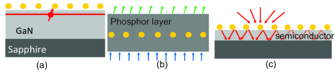
Figure 1: Sketches of canonical scenarios that our theory can address. (a) Plasmonic lattice patterned on a GaN material based LED structure to improve outcoupling; (b) Remote phosphor for white light emission from LED systems, pumped by a blue LED. Plasmonic texturing can improve absorption, and redirect emission. (c) thin film solar cell with texturing to improve light incoupling.

II Theory

Our overall strategy to build a theoretical model is the following. First, we set up a general theory for interaction between dipolar scatterers embedded in a complex dielectric environment. The scatterers are captured in a polarizability, while the interactions are quantified by a Green function. We focus on stratified systems, meaning that the Green function can be built in an angular spectrum representation, separating TE and TM waves. As next step, we determine how to solve for interactions in infinite lattices using Ewald summation, on the proviso that the excitation field is not localized, but rahter has some definite parallel momentum, as would be provided in a plane-wave scattering experiment. Finally we discuss how to obtain the response to localized driving from superposition of the momentum-space solution by the Array Scanning Method (ASM). Section II.1 introduces the Green function, section II.2 sets up the infinite-lattice dipole problem in momentum space, and section II.3 introduces the array scanning method. In section II.4 we discuss an asymptotic expression for evaluating far field radiation, and for calculating the local density of states via reciprocity.

II.1 Dyadic Green’s function for a single magnetoelectric point dipole

For self-consistency, we start from the definition of the Green’s tensor LeePiers2007 ; Novotny2006 , which reads,

$$[\nabla\times\nabla\times-k_{0}^{2}\bar{\bm{\varepsilon}}_{r}(\bm{r})\bar{\bm{\mu}}_{r}(\bm{r})]\bar{\bm{G}}^{ee}(\bm{r},\bm{r}^{\prime})=\bar{\bm{I}}_{0}\delta(\bm{r}-\bm{r}^{\prime}),$$ (1a)

$$[\nabla\times\nabla\times-k_{0}^{2}\bar{\bm{\varepsilon}}_{r}(\bm{r})\bar{\bm{\mu}}_{r}(\bm{r})]\bar{\bm{G}}^{he}(\bm{r},\bm{r}^{\prime})=\bar{\bm{I}}_{0}\nabla\times\delta(\bm{r}-\bm{r}^{\prime}),$$ (1b)

$$[\nabla\times\nabla\times-k_{0}^{2}\bar{\bm{\varepsilon}}_{r}(\bm{r})\mu_{r}(\bm{r})]\bar{\bm{G}}^{hh}(\bm{r},\bm{r}^{\prime})=\bar{\bm{I}}_{0}\delta(\bm{r}-\bm{r}^{\prime}),$$ (1c)

$$[\nabla\times\nabla\times-k_{0}^{2}\bar{\bm{\varepsilon}}_{r}(\bm{r})\mu_{r}(\bm{r})]\bar{\bm{G}}^{eh}(\bm{r},\bm{r}^{\prime})=-\bar{\bm{I}}_{0}\nabla\times\delta(\bm{r}-\bm{r}^{\prime}),$$ (1d)

where $\bar{\bm{G}}^{(e/h)e}$ denotes the electric/magnetic field Green’s tensor from an electric point source, and $\bar{\bm{G}}^{(e/h)h}$ denotes electric/magnetic field Green’s tensor from a magnetic point source. The fields provided by an object with electric current $\bm{j}_{e}(\bm{r})$ and magnetic current $\bm{j}_{h}(\bm{r})$ are given by

$$\begin{aligned} \bm{E}(\bm{r})&=i\omega_{0}\mu_{0}\int\bar{\bm{G}}^{ee}(\bm{r},\bm{r}^{\prime})\bar{\bm{\mu}}_{r}(\bm{r}^{\prime})\bm{j}_{e}(\bm{r}^{\prime})d\bm{r}^{\prime}\\ &+\frac{1}{\bar{\bm{\epsilon}}_{r}(\bm{r})}\int\bar{\bm{G}}^{eh}(\bm{r},\bm{r}^{\prime})\bar{\bm{\epsilon}}_{r}(\bm{r}^{\prime})\bm{j}_{h}(\bm{r}^{\prime})d\bm{r}^{\prime}\\ \bm{H}(\bm{r})&=i\omega_{0}\varepsilon_{0}\int\bar{\bm{G}}^{hh}(\bm{r},\bm{r}^{\prime})\bar{\bm{\varepsilon}}_{r}(\bm{r}^{\prime})\bm{j}_{h}(\bm{r}^{\prime})d\bm{r}^{\prime}\\ &+\frac{1}{\bar{\bm{\mu}}_{r}(\bm{r})}\int\bar{\bm{G}}^{he}(\bm{r},\bm{r}^{\prime})\bar{\bm{\mu}}_{r}(\bm{r}^{\prime})\bm{j}_{e}(\bm{r}^{\prime})d\bm{r}^{\prime}.\end{aligned}$$ (2)

In this work we focus on scatterers that can be modelled as point dipoles, requiring that they are moderate in size (order $\lambda/2\pi$) and sufficiently spaced (spacing at least the particle radius). Although the examples that we present all deal with plasmonic scatterers that only have an electric polarizability, for completeness we also incorporate a magnetic dipole response in the model. Thereby, the model also applies to many metasurfaces. For a point scatterer, the induced electric and magnetic dipole moments $\bm{P}$ and $\bm{M}$ can be expressed in terms of induced currents through $\bm{j}_{e}(\bm{r})=-i\omega_{0}\bm{P}\delta(\bm{r}-\bm{r}_{0})$, $\bm{j}_{h}(\bm{r})=-i\omega_{0}\bm{M}\delta(\bm{r}-\bm{r}_{0})$. Using normalized fields $[\bm{e},\bm{h}]=[\bm{E},Z_{0}\bm{H}]$ and normalized dipole moments $[\bm{p},\bm{m}]=[\frac{\bm{P}}{4\pi\epsilon_{0}},\frac{Z_{0}\bm{M}}{4\pi\mu_{0}}]$ (tantamount to using CGS units), one can simplify the fields due to an arbitrary electric and magnetic dipole scatterer as

$$\begin{pmatrix}\bm{e}\\ \bm{h}\\ \end{pmatrix}=4\pi k_{0}\left(\begin{array}[]{cc}k_{0}\bar{\bm{\mu}}_{r}^{e}\bar{\bm{G}}^{ee}&-i\frac{\bar{\bm{\epsilon}}(\bm{r}_{0})}{\bar{\bm{\epsilon}}(\bm{r})}\bar{\bm{G}}^{eh}\\ -i\frac{\bar{\bm{\mu}}(\bm{r}_{0})}{\bar{\bm{\mu}}(\bm{r})}\bar{\bm{G}}^{he}&k_{0}\bar{\bm{\varepsilon}}_{r}^{e}\bar{\bm{G}}^{hh}\end{array}\right)\begin{pmatrix}\bm{p}\\ \bm{m}\\ \end{pmatrix}.$$ (3)

In this work we focus on lattices embedded in planar photonic structures, consisting of an arbitrary multilayer stack. In this case, to construct the multilayer Green function one uses plane waves, decomposed into TM and TE polarization for each given propagation direction, as specified by parallel momentum $\mathbf{k}_{||}$ (momentum component in the plane parallel to the interfaces) as a complete basis to describe any field in space. By convention, this set of plane waves is expressed through a set of basis functions $\bm{M}(\bm{k}_{||})$ defined as describing the electric field of TE waves, and a dual set ($\bm{N}(\bm{k}_{||})$) that describes the electric field of TM waves. One set of basis functions can be derived from the other since $\bar{\bm{G}}^{ee}=\bar{\bm{G}}^{hh}$, the $\bm{M}(\bm{k}_{||})$ functions not only describe the E-field of TE waves, but also describe the TM-wave $H$-fields. From the relation between E-field and H-field in source-free regions, $\bar{\bm{G}}^{eh}(\bm{r},\bm{r}^{\prime})=-\nabla\times\bar{\bm{G}}^{hh}(\bm{r},\bm{r}^{\prime})$, one finds $\nabla\times\bm{M}(\bm{k}_{||})=k_{0}\bm{N}(\bm{k}_{||})$. Conversely, one can also derive $\nabla\times\bm{N}(\bm{k}_{||})=k_{0}\bm{M}(\bm{k}_{||})$, where curl operates on the coordinates of detection point $\bm{r}$. This relation facilitates a straightforward computation of all sub-tensors of $\bar{\bm{G}}$ in terms of $\bm{M}(\bm{k}_{||})$ and $\bm{N}(\bm{k}_{||})$. The appendices report the functions $\bm{M}(\bm{k}_{||})$ and $\bm{N}(\bm{k}_{||})$ for free space (Appendix A, essentially plane waves), and for arbitrary stratified systems. In any multilayer structure, the functions $\bm{M}(\bm{k}_{||})$ and $\bm{N}(\bm{k}_{||})$ can be found by applying the transfer matrix formalism, that introduces the wave-vector dependent fresnel coefficients into the problem. Appendix C generalizes the aforementioned reported recipe KlimovPRA2005 ; HartmanJCP ; Cheng1986 for Green’s tensor $\bar{\bm{G}}^{ee}$ to the complete description of the $\bm{E}$ and $\bm{H}$ fields induced by a single magneto-electric point scatter.

II.2 2D lattice and plane wave excitation

We now turn to the case of a 2D periodic magneto-electric point scatter lattice coupled to a slab waveguide under a plane wave illumination. We consider the response of a 2D lattice (lattice vectors $\bm{R}_{\bm{l}}=m\bm{a}_{1}+n\bm{a}_{2}$) of point dipoles of polarizability $\bar{\bm{\alpha}}$ to a driving field of parallel wave vector $\bm{k}_{||}$, where we index lattice sites with the label $\bm{l}=[m,n]$. The response is set by solving a self-consistent coupled equation given by

$$\begin{pmatrix}\bm{p}_{\bm{l}}\\ \bm{m}_{\bm{l}}\end{pmatrix}=\bar{\bm{\alpha}}\left[\left(\begin{array}[]{c}\bm{e}^{\bm{k}_{||}}(\bm{R}_{\bm{l}})\\ \bm{h}^{\bm{k}_{||}}(\bm{R}_{\bm{l}})\end{array}\right)+\sum\limits_{\bm{l}^{\prime}\neq\bm{l}}\bar{\bm{g}}(\bm{R}_{\bm{l}},\bm{R}_{\bm{l}^{\prime}})\begin{pmatrix}\bm{p}_{\bm{l}^{\prime}}\\ \bm{m}_{\bm{l}^{\prime}}\end{pmatrix}\right].$$ (4)

where $\bar{\bm{\alpha}}$ is the dynamic polarizability tensor, $\bar{\bm{g}}(\bm{R}_{\bm{l}},\bm{R}_{\bm{l}^{\prime}})=4\pi\left(\begin{array}[]{cc}k_{0}^{2}{\bm{G}}^{ee}(\bm{R}_{\bm{l}},\bm{R}_{\bm{l}^{\prime}})&-ik_{0}\bar{\bm{G}}^{eh}(\bm{R}_{\bm{l}},\bm{R}_{\bm{l}^{\prime}})\\ -ik_{0}\bar{\bm{G}}^{he}(\bm{R}_{\bm{l}},\bm{R}_{\bm{l}^{\prime}})&k_{0}^{2}\bar{\bm{G}}^{hh}(\bm{R}_{\bm{l}},\bm{R}_{\bm{l}^{\prime}})\end{array}\right)$, and where $\bm{p}_{\bm{l}}$ ($\bm{m}_{\bm{l}}$ ) represents the induced electric (magnetic) dipole moment in the point scatter seated at $\bm{R}_{\bm{l}}$. By using the stratified medium dyadic Green’s function $\bar{\bm{g}}(\bm{r},\bm{r}^{\prime})$, given in Appendix Eq. (18), we ensure that all multiple scattering interactions between the induced dipole moments $\bm{p}_{\bm{l}}$ that are mediated by both propagating and guided modes are included. The driving field $\bm{e}^{\bm{k}_{||}}(\bm{R}_{\bm{l}})$ ($\bm{h}^{\bm{k}_{||}}(\bm{R}_{\bm{l}})$) is understood to be the field solution for the full stratified system in absence of the nanoscatterers in response to an incident plane wave $\bm{E}_{in}^{0}$ of parallel momentum $\bm{k}_{||}$, as specified in Urbach1998 ; Jung2011 . According to de Vries et al. Vries1998 , the dynamical polarizability tensor $\bar{\bm{\alpha}}$ of a point scatter can be written as $\bar{\bm{\alpha}}=\left[\bar{\alpha}_{static}^{-1}-4\pi k^{2}\bar{\bm{G}}_{b}(\bm{r}_{0},\bm{r}_{0})\right]^{-1}$, where $\bar{\alpha}_{static}$ is a quasistatic polarizability (no radiation damping), and where $\bar{\bm{G}}_{b}$ is the background Green’s tensor at the position of the point scatter itself. A regularization procedure needs to be carried out to remove the singularity in $\real\bar{\bm{G}}_{b}$. Since this regularization is not specific to the stratified system, we refer to Ref. Vries1998, for its derivation. For a point scatterer in free space, the routine boils down to taking solely the imaginary part of $\bar{\bm{G}}_{b}$, which accounts for the radiation damping to fulfill the optical theorem. In a complex system, one corrects the polarizability tensor of a point scatter by adding to the inverse static polarizability $4\pi k^{2}i\mathrm{Im}\bar{\bm{G}}_{free}$ (referring to the Green function of homogeneous space filled with the medium directly surrounding the scattering), plus the scattered part $4\pi k^{2}{\bar{\bm{G}}_{s}(\bm{r}_{0},\bm{r}_{0})}$ of the Green’s tensor that contains all the multiple reflections in the multilayer stack, and is regular. Mathematically, one adds to the inverse of static polarizability, i.e., $\alpha^{-1}=\alpha_{static}^{-1}-\frac{2ik^{3}}{3}\bar{\bm{I}}_{0}-{\bar{\bm{G}}_{s}(\bm{r}_{0},\bm{r}_{0})}$.

Returning to Eq. (4), the translation invariance of the coupled lattice-waveguide system implies that a Bloch wave form $\left[\bm{p}_{\bm{l}},\bm{m}_{\bm{l}}\right]^{T}=e^{i\bm{k}_{||}\cdot\bm{R}_{\bm{l}}}\left[\bm{p}_{\bm{0}},\bm{m}_{\bm{0}}\right]^{T}$ can be used to simplify the infinite set of coupled equations to a single equation

$$\begin{pmatrix}\bm{p}_{\bm{0}}\\ \bm{m}_{\bm{0}}\end{pmatrix}=[\bar{\bm{\alpha}}^{-1}-\bm{g}^{\neq}]^{-1}\begin{pmatrix}\bm{E}_{in}(\bm{R}_{\bm{0}})\\ \bm{H}_{in}(\bm{R}_{\bm{0}})\end{pmatrix},$$ (5)

where $\bar{\bm{g}}^{\neq}$ is the lattice summation of the stratified system Green’s function without self-term, given by $\bar{\bm{g}}^{\neq}=\sum\limits_{\bm{l}\neq\bm{0}}\bar{\bm{g}}(\bm{R}_{\bm{0}},\bm{R}_{\bm{l}})e^{i\bm{k}_{||}\cdot\bm{R}_{\bm{l}}}$, $\bm{R}_{0}$ is the coordinates of the particle labeled by $\bm{l}=[0,0]$ on the lattice. Even for dipole interactions in free space, it is a challenge to calculate the lattice sum $\bar{\bm{g}}^{\neq}$, which can be tackled using Ewald summation techniques. We have adapted the recipe of Linton Linton2010 for summations involving just scalar Green functions in free space to deal also with dyadic Green functions of arbitrary stratified systems. To this end, we reformulate the total Green’s tensor of stratified structures as $\bar{\bm{g}}(\bm{r},\bm{r}^{\prime})=\bar{\bm{g}}_{0}(\bm{r},\bm{r}^{\prime})+\bar{\bm{g}}_{s}(\bm{r},\bm{r}^{\prime})$, where $\bar{\bm{g}}_{0}$ and $\bar{\bm{g}}_{s}$ are the free space term and the scattered term due to the interfaces, respectively. The explicit form of $\bar{\bm{g}}_{0}$ and $\bar{\bm{g}}_{s}$ can be seen in Appendix(A-C). This separation of $\bar{\bm{g}}(\bm{r},\bm{r}^{\prime})$ leads to

$$\bar{\bm{\alpha}}^{-1}-\bar{\bm{g}}^{\neq}(\bm{k}_{||}) =\bar{\bm{\alpha}}_{static}^{-1}-\frac{2ik^{3}}{3}-\sum\limits_{\bm{l}}\bar{\bm{g}}_{s}(\bm{R}_{\bm{0}},\bm{R}_{\bm{l}})e^{i\bm{k}_{||}\cdot\bm{R}_{\bm{l}}}$$ (6)

$$-\{\sum\limits_{\bm{l}}\bar{\bm{g}}_{0}(\bm{R}_{\bm{0}},\bm{R}_{\bm{l}})e^{i\bm{k}_{||}\cdot\bm{R}_{\bm{l}}}-\bar{\bm{g}}_{0}(\bm{R}_{\bm{0}},\bm{R}_{\bm{0}})\}.$$

The ‘free’ term (entire term in $\{.\}$) in Eq. (6) can be efficiently calculated using Ewald summation. We use the recipe reported in Ref PerPRB2013, ; KwadrinPRB2014, . At first sight, the summation over $\bar{\bm{g}}_{s}$ in the third term in Eq. (6) must be much more daunting, since the scattered part of the Green function is formulated as a Sommerfeld integral over parallel wavector containing the $\mathbf{M}$ and $\mathbf{N}$ modes of the multilayer. Remarkably, the sum of poorly convergent complex integrals simplifies to a rapidly converging sum of just the integrand at select $\bm{k}_{||}$ that rapidly converges due to the evanescent nature of the higher diffraction orders. Taking one block in $\bar{\bm{g}}_{s}$ for an interface as an example, we explicitly formulate $\sum\limits_{\bm{l}}\bar{\bm{G}}_{s}^{ee}(\bm{R}_{\bm{0}},\bm{R}_{\bm{l}})e^{i\bm{k}_{||}\cdot\bm{R}_{\bm{l}}}$ for the example of a lattice placed on top of a slab waveguide as follows,

$$\sum\limits_{\bm{l}}\bar{\bm{G}}_{s}^{ee}(\bm{R}_{\bm{0}},\bm{R}_{\bm{l}})e^{i\bm{k}_{||}\cdot\bm{R}_{\bm{l}}}=\sum\limits_{\bm{l}}\iint_{\infty}^{\infty}dq_{x}dq_{y}\frac{i}{8\pi^{2}k_{z1}}$$ (7)

$$[{\bm{M}_{+}\otimes\gamma_{s}^{1,23}\bm{M}^{\prime}_{+}}+{\bm{N}_{+}\otimes\gamma_{p}^{1,23}\bm{N}^{\prime}_{+}}]e^{-i\bm{q}_{||}\cdot(\bm{R}_{\bm{l}}-\bm{R}_{\bm{0}})}e^{i\bm{k}_{||}\cdot\bm{R}_{\bm{l}}}.$$

Here we refer to the Appendix for a listing of the quantities involved - essentially $\gamma_{s,p}^{1,23}$ accounts for the polarization-dependent fresnel coefficients of the multilayer system, generalized to extend to large $k_{||}$. The crucial realisation is that in this complicated integrand there is no dependence on $\mathbf{R}_{l}$ except in the very last term, i.e., the phase factor $e^{i(\bm{k}_{||}-\bm{q}_{||})\cdot\bm{R}_{\bm{l}}}$. Hence one can pull the summation over lattice sites into the integrand and apply the completeness relation $\sum\limits_{\bm{l}}e^{i(\bm{k}_{||}-\bm{q}_{||})\cdot\bm{R}_{\bm{l}}}=\frac{(2\pi)^{2}}{A}\sum\limits_{\bm{l}}\delta((\bm{k}_{||}-\bm{q}_{||})-\bm{\mathscr{G}}_{\bm{l}})$ (where $\bm{\mathscr{G}}_{\bm{l}}=m\bm{\mathscr{G}}_{x}+n\bm{\mathscr{G}}_{y}$, $\bm{\mathscr{G}}_{x}$ and $\bm{\mathscr{G}}_{y}$ are reciprocal lattice vectors and $A$ denotes the real-space unit cell area) to convert the real space summation of integrals in Eq. (7) into a reciprocal space sum with no complex integrals as follows,

$$\sum\limits_{\bm{l}}\bar{\bm{G}}_{s}^{ee}(\bm{R}_{\bm{0}},\bm{R}_{\bm{l}})e^{i\bm{k}_{||}\cdot\bm{R}_{\bm{l}}}=\frac{(2\pi)^{2}}{A}\sum\limits_{\bm{l}}\frac{i}{8\pi^{2}k_{z2}}$$ (8)

$$[{\bm{M}_{+}\otimes\gamma_{s}^{1,23}\bm{M}^{\prime}_{+}}+{\bm{N}_{+}\otimes\gamma_{p}^{1,23}\bm{N}^{\prime}_{+}}]e^{i\bm{k}_{||}\cdot\bm{R}_{\bm{0}}}|_{(\bm{q}_{||}=\bm{k}_{||}+\bm{\mathscr{G}}_{\bm{l}})}.$$

In Eq. (8), the sum can be easily truncated (despite the existence of guided modes with a very long in-plane real-space range), due to the fact that each term carries a $e^{i2k_{z}d}$ ($d$ denotes the distance of particle center to its nearest neighboring interface), which exponentially decreases as $|{\bm{k}}_{||}+{\mathscr{G}}_{\bm{l}}|$ is large enough. The same rationale holds for all blocks in $\bar{\bm{g}}_{s}$. Once the induced moment $\bm{p}_{\bm{0}}$ and $\bm{m}_{\bm{0}}$ is obtained, it is straightforward to calculate the total field at any location as

$$\begin{pmatrix}\bm{E}_{total}^{\bm{k}_{||}}(\bm{r})\\ \bm{H}_{total}^{\bm{k}_{||}}(\bm{r})\end{pmatrix}=\begin{pmatrix}\bm{E}_{slab}^{\bm{k}_{||}}(\bm{r})\\ \bm{H}_{slab}^{\bm{k}_{||}}(\bm{r})\end{pmatrix}+\sum\limits_{\bm{l}}\bar{\bm{g}}(\bm{r},\bm{R}_{\bm{l}})e^{i\bm{k}_{||}\cdot\bm{R}_{\bm{l}}}\begin{pmatrix}\bm{p}_{\bm{0}}\\ \bm{m}_{\bm{0}}\end{pmatrix}.$$ (9)

II.3 Point dipole excitation

We proceed to discuss the coupled lattice-waveguide under a point source excitation by employing the array scanning method (ASM) reviewed, for instance, by Capolino et al. in Capolino2007 . The use of Bloch’s theorem, and the Ewald lattice summation technique, as we presented sofar, restricts one to finding the response to extended driving field of definite parallel momentum, as it requires periodicity of the entire system (geometry plus driving) under study. In principle, one can decompose the driving by a single point source in plane waves, and thereby obtain the response of a lattice to local driving by superposition. More practical for implementation is the Array Scanning Method which states that a single point source can be constructed from integration over phased arrays of sources Capolino2007 . Provided one can solve for any well-defined phased array $J_{\bm{k}_{||}}=\bm{J}\sum\delta(\bm{r}-(\bm{r}^{\prime}+\bm{R}_{\bm{l}}))e^{i\bm{k}_{||}\cdot\bm{R}_{\bm{l}}}$ of definite parallel momentum, and the same periodicity as the lattice, one can retrieve the single point dipole source by integrating $J_{\bm{k}_{||}}$ over the Brillouin zone, i.e., $\bm{J}(\bm{r}^{\prime})=\frac{A}{(2\pi)^{2}}\int\limits_{BZ}\bm{J}_{\bm{k}_{||}}d\bm{k}_{||}$. For each individual $\bm{k}_{||}$, the problem is directly compatible with the formulation that was set up for plane wave excitation. When summing the results over all $\bm{k}_{||}$, one has to ensure each $\bm{k}_{||}$ receives its own weighting, as given by the background Green’s tensor. The central result of this approach is that the field due to a point source is

$$\bar{\bm{G}}(\bm{r},\bm{r}^{\prime})=\bar{\bm{g}}_{b}(\bm{r},\bm{r}^{\prime})+\frac{A}{(2\pi)^{2}}\int\limits_{BZ}d\bm{k}_{||}\bar{\bm{I}}(\bm{k}_{||},\bm{r},\bm{r}_{0})$$ (10)

where $\bar{\bm{g}}_{b}(\bm{r},\bm{r}^{\prime})$ is the background dyadic green function (i.e., that of the stratified system in absence of the lattice), the integrand of the second term $\bar{\bm{I}}(\bm{k}_{||},\bm{r},\bm{r}_{0})$ is given by $\bar{\bm{I}}(\bm{k}_{||},\bm{r},\bm{r}_{0})=\bm{g}^{=}(\bm{r},\bm{r}_{0})\bar{\bm{Q}}(\bm{r}_{0},\bm{r}_{0})\bm{g}^{=}(\bm{r}_{0},\bm{r}^{\prime})$, and $\bm{g}^{=}(\bm{r}_{0},\bm{r}^{\prime})=\sum\limits_{\bm{l}}\bar{\bm{g}}(\bm{r}_{0},\bm{r}^{\prime})e^{i\bm{k}_{||}\cdot\bm{R}_{\bm{l}}}$ is again a lattice-summed Green function, though now including the self-term, i.e., $\bm{l}=\bm{0}$ term. The interpretation of $\bar{\bm{I}}(\bm{k}_{||},\bm{r},\bm{r}_{0})$ is that the first term gives direct radiation from the source without interaction with the lattice. The second term contains the emission scattered via the lattice, and is the term containing the array scanning. The integrand of second term has three factors, that should be read from right to left:

1. $\bm{g}^{=}(\bm{r}_{0},\bm{r}^{\prime})=\sum\limits_{\bm{l}}\bar{\bm{g}}(\bm{r}_{0},\bm{r}^{\prime})e^{i\bm{k}_{||}\cdot\bm{R}_{\bm{l}}}$, gives the field strength at the particle lattice site $\bm{r}_{0}$ excited by the array of discrete current source $\bm{J}e^{i\bm{k}_{||}\cdot\bm{R}_{\bm{l}}}$ located at $\bm{r}^{\prime}+\bm{R}_{\bm{l}}$,

2. $\bar{\bm{Q}}=[\bar{\bm{\alpha}}^{-1}-\bar{\bm{g}}^{\neq}(\bm{k}_{||})]^{-1}$ quantifies how much the lattice is polarized by the phased array source $\bm{J}e^{i\bm{k}_{||}\cdot\bm{R}_{\bm{l}}}$,

3. $\bm{g}^{=}(\bm{r},\bm{r}_{0})=\sum\limits_{\bm{l}}\bar{\bm{g}}(\bm{r},\bm{r}_{0})e^{i\bm{k}_{||}\cdot\bm{R}_{\bm{l}}}$, describes the field strength at $\bm{r}$ of field radiated by the polarized lattice.

The calculation of $\bar{\bm{g}}^{=}(\bm{r},\bm{r}_{0})$ and $\bar{\bm{g}}^{=}(\bm{r}_{0},\bm{r}^{\prime})$ can be performed by applying the completeness relation as discussed for $\bar{\bm{g}}^{\neq}(\bm{r}_{0},\bm{r}_{0})$. A major difference, however, is that now the source point $\bm{r}_{0}$ might be in a different layer than the lattice, as opposed to the lattice sum appearing for particle-particle interactions. An apparent problem is that the Green’s tensor introduces $1/k_{nz}$ terms, which introduce a singularity at the light line for medium $n$. Detailed analysis shows that the $1/k_{1z}$ in the Green’s tensor cancels out with the $k_{1z}$ proportionality of the fresnel transmission coefficient, which removes the numerical singularity. As example, consider a three-layer system, with an emitter in layer $1$ ($\bm{r}^{\prime}=[0,0,z^{\prime}]$), while the particle lattice is in layer 2, so that we need a corresponding dyadic Green tensor that accounts for the field propagation across the interface through a generalized fresnel transmission coefficient. We take only one block in $\bar{\bm{g}}_{b}(\bm{r},\bm{r}^{\prime})$, e.g., $\bar{\bm{G}}_{slab}^{{EE,21}}(\bm{r}_{0},\bm{r}^{\prime})$, to illustrate this useful cancellation result, which is given by

$$\bar{\bm{G}}_{slab}^{{EE,21}}(\bm{r}_{0},\bm{r}^{\prime})=\iint dk_{x}dk_{y}\frac{i}{8\pi^{2}}\{$$ (11)

$$\frac{1}{\Delta_{s}}\{[\bm{M}_{-}(\bm{k}_{||})+\gamma_{s,23}(k_{||})\bm{M}_{+}(\bm{k}_{||})]T_{s,12}e^{i\psi}\}\otimes[\bm{M}^{\prime}_{+}(\bm{k}_{||})]$$

$$-\frac{1}{\Delta_{p}}\{[\bm{N}_{-}(\bm{k}_{||})+\gamma_{p,23}(k_{||})\bm{N}_{+}(\bm{k}_{||})]T_{p,12}e^{i\psi}\}\otimes[\bm{N}^{\prime}_{+}(\bm{k}_{||})]\}$$

where $T_{s,ij}=\frac{2}{k_{zi}+k_{zj}}$, and $T_{p,ij}=\frac{2\sqrt{\epsilon_{i}\epsilon_{j}}}{k_{zi}\epsilon_{j}+k_{zj}\epsilon_{i}}$, $\psi=(k_{2z}-k_{1z})d$. Importantly, such cancellations carry over to complex layered structures, meaning that numerical calculation greatly benefits from judicious ordering of terms.

As regards to performing the integrations over the Brillouin zone of the type above, we note that even if the $1/k_{nz}$ singularities are eliminated, singularities still can occur due to poles in the transmission coefficients at ${\bm{k}}_{||}$ that match guided modes of the stratified system. We implemented a finite element scheme to efficiently carry out the numerical integration. The basic idea is to discretize the integration domain into triangles on which a simple quadrature rule is evaluated, and to adaptively refine the triangle density to obtain convergence also at guided mode contributions.

II.4 Far field asymptotic form and radiative LDOS

So far we discussed how to solve for the response of scattering particle lattices to extended and local excitation, without going into the question how to calculate far field observables. Using far field asymptotic forms of Eq. (9) enables one to calculate transmission, reflection, diffraction efficiency, and absorption with ease for any incident parallel momentum. The asymptotic form of Eq. (9) can be obtained Novotny2006 by,

$$\bm{E}_{\infty}(s_{x},s_{y},s_{z})=-2i\pi k_{z}\bm{E}(k_{x},k_{y};z=z_{r})\frac{e^{ikr}}{r}$$ (12)

where $\bm{s}=[s_{x},s_{y},s_{z}]=[\frac{x}{r},\frac{y}{r},\frac{z}{r}]=[\frac{k_{x}}{k_{0}},\frac{k_{y}}{k_{0}},\frac{k_{z}}{k_{0}}]$ parametrizes the far-field ‘viewing direction’, and where $\bm{E}(k_{x},k_{y};z=z_{r})$ is the angular spectrum of the near field at an arbitrarily chosen detection plane $z=z_{r}$ in the half-space that extends to the far field detector. For plane wave incidence with in plane wave vector $\bm{k}_{||}$, the only Fourier components of $\bm{E}(k_{x},k_{y};z=z_{r})$ contributing to the far field are at $[k_{x},k_{y}]=[\bm{k}_{||}+\bm{\mathscr{G}}_{\bm{l}}]$ ,where $\bm{l}$ labels the discrete diffraction orders.

In this work we are particularly concerned with mapping the fractional, i.e., parallel wave-vector resolved, radiative local density of states, i.e., the radiated flux per solid angle in the far field that is due to a localized source. In the ASM scheme, the asymptotic form of the far field Green’s function can be approximated from Eq. (10) by taking the angular spectrum at a reference plane $z=z_{r}$,

$$\bar{\bm{g}}^{far}([k_{x},k_{y},z=z_{r}],\bm{r}^{\prime})=\bar{\bm{g}}_{b}([k_{x},k_{y},z=z_{r}],\bm{r}^{\prime})$$ (13)

$$+\frac{A}{(2\pi)^{2}}{\bm{g}}^{=}_{\bm{l}=\bm{0}}([k_{x},k_{y},z=z_{r}],\bm{r}_{0})\bar{\bm{Q}}(\bm{r}_{0},\bm{r}_{0}){\bm{g}}^{=}(\bm{r}_{0},\bm{r}^{\prime})$$

for radiation at an output angle given by $[k_{x}/k_{0},k_{y}/k_{0}]=cos\theta[cos\phi,sin\phi]$. Here the term $\bar{\bm{g}}_{b}([k_{x},k_{y},z=z_{r}],\bm{r}^{\prime})$ represents the far field emitted directly by the source (no interaction with the lattice). The second term accounts for radiation that appears via interaction with the lattice. It contains three sub-terms multiplicating with each other: the first sub-term $\bar{\bm{g}}^{=}(\bm{r}_{0},\bm{r}^{\prime})$ accounts for how strongly the source drives the lattice, the second sub-term $\bar{\bm{Q}}$ plays the role of polarizability, and the final sub-term $\bar{\bm{g}}^{=}_{\bm{l}=0}$ quantifies how each particle in the lattice scatters out. Explicit expressions of ${\bm{g}}^{=}(\bm{r}_{0},\bm{r}^{\prime})$ and $\bar{\bm{Q}}(\bm{r}_{0},\bm{r}_{0})$ are given in Eq. (10), while the term ${\bm{g}}^{=}_{\bm{l}=0}([k_{x},k_{y},z=z_{r}],\bm{r}_{0})$ only takes the zero diffraction order, i.e., $\bm{l}=\bm{0}$. We can use Eq. (13) to calculate the radiative local density of states by taking the sampling points of $\bm{k}_{||}$ within the light cone, without the need of unfolding $\bm{k}_{||}$ into corresponding diffraction orders for large pitches (larger than half wavelength), compared to sampling points taken from Brillouin zone.

An independent method to obtain the radiative local density of states is to use the reciprocity theorem. Reciprocity implies that the local field enhancement inside the waveguide upon far field plane wave illumination is equivalent to calculating the plane wave strength in the far field due to a localized source Janssen_OE_2010 . Strictly, one needs to identify the local electric field enhancement in the waveguide, upon far field plane wave illumination weighted by a factor of $\frac{1}{k_{z}}$ with the fractional radiative local density of states enhancement. Hence, one can calculate the far field emission pattern of a localized source coupled to the lattice-waveguide simply by calculating the local field at the emitter position due to a plane wave scattered by the coupled lattice-waveguide, incident from the direction of interest. The reciprocity technique can be easily extended to a bulk light source, i.e., emitters randomly distributed inside the waveguide in a certain region, by integrating $|E|^{2}$ over the active area RodriguezPRB2014 to efficiently obtain the far field emission pattern. However, the disadvantage of the reciprocity method is that it will not allow to determine the guided-mode contribution to LDOS, nor of absorption induced by the lattice. Any contribution to LDOS (imaginary part of the full system Green dyadic) that does not appear as far field power, is not accessible to the reciprocity method. Thereby both the ASM and reciprocity are useful, and provide complementary information.

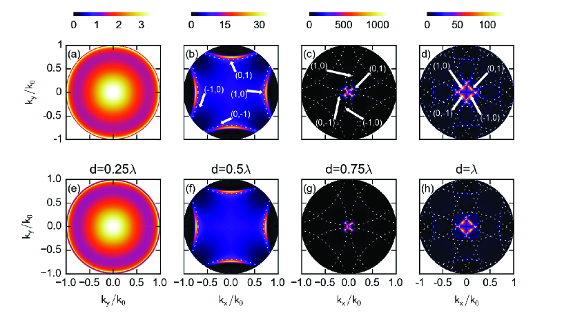
Figure 2: Angle-dependent far-field emission enhancement of an electric dipole located insidea slab waveguide coupled to a plasmonic lattice, as sketched in Fig. 1 (a). The host medium of the lattice is air, below which a waveguiding layer (index 1.6, thickness 0.2$\lambda_{0}$) is placed on a perfect reflector. a-d (e-h) shows emission pattern calculated from ASM method (reciprocity method) at four lattice constants, i.e., $1/4\lambda_{0}$, $1/2\lambda_{0}$, $3/4\lambda_{0}$, $\lambda_{0}$ respectively. $\lambda_{0}$ is the vacuum wavelength. White lines are the folded slab waveguide inside the light cone. In (b,c,d), the white number pairs denote the diffraction order. The nanoparticle is taken as metallic sphere defined through an electrostatic polarizability of $(3.78+0.135i)\cdot 10^{-3}\lambda_{0}^{3}$ (typical for, e.g., a 80 nm aluminum particle in the green). The calculation is done for a single frequency determined by $2\pi/\lambda_{0}$, and taking a source height $Z_{0}=1/10\lambda_{0}$.

III Results and discussion

III.1 Comparison of the far field pattern between reciprocity method and ASM scanning method

We consider the fractional radiative local density of optical states (FLDOS) in a scenario similar to that recently explored by Lozano et al. Lozano2013 and Rodriguez et al. RodriguezPRB2014 for improvement of white light generation in thin phosphors that are excited by blue LEDs. In this scenario, a random ensemble of emitters in a thin layer of moderate index (about 1.5) is coupled to a lattice of plasmon particles to benefit from ”diffractive ”surface lattice resonances, and diffractive outcoupling of light emitted into waveguide modes. ExperimentsLozano2013 ; RodriguezPRB2014 in particular showed highly directional emission (several degrees wide emission cone) into angles matching grating outcoupling of waveguided modes. Here we present calculations of the fractional radiative LDOS for four different lattice pitches, to at the same time demonstrate the applicability of the point dipole model, and compare the ASM method to the reciprocity method. In Fig. 2 we consider the angle-dependent far-field emission enhancement for a single emitter coupled to this waveguide-lattice structure, divided by the emission of a bare emitter in the same slab structure without particles.

As stratified system we take a n=1.6 slab (the phosphor) positioned on a perfect electric conductor, and a thickness that is 1/5th of the free space emission wavelength (550 nm, green emission), i.e., 110 nm. As particles we take metal nanoparticles placed on the slab, where the particles are defined through a static polarizability $\bar{\alpha}_{static}=(3.78+0.135i)\cdot 10^{-3}\lambda_{0}^{3}$ (typical for, e.g., 80 nm Aluminum particles in the green). For this example we consider a single source position and orientation, although for actual phosphors one would need to perform incoherent averaging over all source positions and orientations. For this example, we consider the source as an electric dipole moment perpendicular to the interfaces, so that only TM modes are excited. Fig. 2 shows both the angle-dependent far-field emission enhancement calculated according to the ASM method, with assistance of Eq. (13), as shown in Fig. 2 (a,b,c,d), and calculated according to reciprocity, i.e., as a near-field enhancement upon far-field TM-wave illumination, as shown in Fig. 2 (e,f,g,h). Results are shown for four different lattice constants, chosen as $\lambda_{0}/4$ (subdiffractive), $\lambda_{0}/2$ (diffractive), $3\lambda_{0}/4$ (close to 2nd order Bragg diffraction for the waveguide mode) and $\lambda_{0}$.

In Fig. 2 (a,e), the lattice is effectively a dense, non-diffractive metasurface, as the pitch is chosen so small $(\lambda_{0}/4)$ that no diffraction contributes to the far field emission pattern. For this lattice pitch, the directional radiation enhancement appears as a cone of about 30 degree opening angle. Here the reader should be warned that we plot enhancement, and when dividing to obtain photoluminescence enhancement, one divides by the bare dipole emission, which is dark near the vertical for the chosen vertical dipole orientation. As the lattice constant increases, the waveguide mode, with dispersion $\omega=|\mathbf{k}_{||}|n_{\mathrm{mode}}$ diffracts, and by diffraction is partially folded inside the light cone, thus coupling out into the far field. For the larger pitch, emission from the dipole that is emitted into the waveguide mode can hence be collected, and is manifested as bright arcs with a radius of curvature given by the waveguide mode index in Fig. 2 (b,f), and the panel pairs (c,g) and (d,h). For larger pitch, the arcs approach, and show a anticrossing, as the condition of second order Bragg diffraction for the TM waveguide mode is passed. The bright arcs in enhancement follow essentially the repeated-zone scheme folding of the waveguide slab mode dispersion by the plasmonic lattice (waveguide dispersion replicated every reciprocal lattice vector). Compared with the pure waveguide folding as indicated by the white dash lines (unperturbed waveguide dispersion, plotted in repeated zone scheme dispersion, the bright arcs are broadened and slightly shifted. The broadening reflects a finite propagation length of the folded wave guide mode, due to the intrinsic Ohmic losses from the point scatters and the inclusion of radiation damping. As regards the shift of the mode to smaller mode index, we note that the particles push the mode profile out of the high-index material thereby lowering the mode index, shifting features way from the drawn circles. Qualitatively, i.e., in terms of showing sharp features that reflect the hybridized plasmonic-waveguide modes in a repeated zone scheme, the calculations are in good accord with observations made by Lozano et al. and Schokker et al. Lozano2013 ; Schokker2014 . In terms of magnitude of the enhancement, as shown in Fig. 2 (c,g), the predicted FLDOS enhancements are large, of order 100 (panel d) to 1000 (panel (c)). This large value is due to the fact that we use a perpendicular dipole for excitation, which in the bare layer case hardly radiates at small emission angles. Since our results are normalized to the bare dipole donut-shaped emission pattern, this emphasizes emission at small $\mathbf{k}_{||}$ as a pronounced enhancement.

A significant advantage of the reciprocity-based approach is that it requires only plane wave calculations, and that results can be obtained for all source positions and orientations in the unit cell in one calculation. This should be contrasted to the ASM method, that needs a full calculation per dipole position and orientation. However, the reciprocity based method can not separate out contributions to the local density of states that do not result in far field radiation, such as quenching and emission that remains trapped in waveguide modes. As we describe in section III.3, the ASM does provide means to unravel these phenomena. To highlight the calculation speed advantage of the ASM (the slowest of our two methods), over full wave simulations, we give a brief comparison of the computational time of our method and the full-wave simulation package Comsol. For ASM, each frame of the calculation in Fig. 2 (a-d) with 200$\times$100 computation points takes roughly 1 minute. For a similarly complex structure, Comsol will take roughly 1 minute for a single computation point, on similar computer hardware. This significant difference in computational time signifies the efficiency of our method, as it allows to rapidly screen different geometries.

III.2 Photovoltaic system

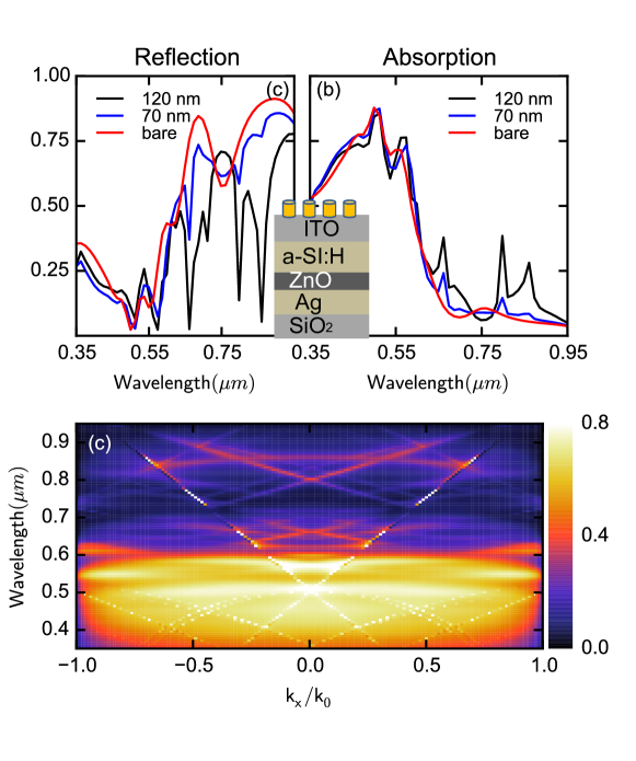
Figure 3: (a) Calculated reflection from the layer geometry shown in the inset, which reflects the cell geometry of a realistic photovoltaic cell based on amorphous silicon LareAPL2012 . (b) Calculated absorption in the a-Si:H i-layer. Red line for the bare layer geometry without plasmonic lattice, blue line for the plasmonic lattice with particle radius of 70 nm, black line for the plasmonic lattice with particle radius of 120 nm. (c) Absorption as function of incident angle and photon energy. In (a-b), light is illuminated at normal incidence. In (c), the incident light has TE polarization.

As second example of the utility of our method we apply our dipole theory to a realistic photovoltaic (PV) structure, in which the plasmonic lattice is coupled to thin-film silicon solar cells containing several layers, as studied by van Lare LareAPL2012 et. al. In particular, the application area is to amorphous silicon (a-Si:H) photovoltaics, in which 350 nm of silicon is sandwiched between an ITO contact, on one side, and a 80 nm ZnO buffer layer to a 200 nm thick silver back contact on the other side. One challenge of such cells is that the silicon is much thinner than the absorption length, especially in the red. Consequently, these cells have up to 80% reflectivity for wavelengths above 650 nm. The aim of plasmonic structuring is to improve absorption in the amorphous silicon layer, despite the fact that it is far thinner than the bulk absorption length, by coupling into guided modes. This example illustrates the potential application of our method to rapidly screen complex photonic structures in thin-film photovoltaics. In the construction of our dyadic Green’s function, we implement the full layer-structure of the thin-film silicon solar cells. However, to a good approximation, we take the 200 nm thick Ag back contact as infinite. We use tabulated optical constants for all materials, taken from LareAPL2012 ; Palik .

Figure 3 (a,b) shows the calculated reflection, absorption in a-Si:H i-layer for the bare layer geometry, and geometries that include embedded plasmonic particle lattices of pitch 500 nm, and two different particle sizes (radius of 70 nm, and 120 nm). In Fig. 3 (a), it is evident that without the plasmonic lattice, the cell shows minimum reflectivity at 550 nm, and a large 80% reflectivity for wavelengths above 650 nm. This is in good accord with the full wave simulations of van Lare, and highlights a main problem of thin film amorhous solar cell, namely that light is reflected at the back contact after a single pass, without being absorbed. The plasmonic lattices strongly reduce the cell reflection in a set of narrow spectral lines, where the introduced reflection minima are most pronounced for the larger particles, again in good accord with the work of van Lare LareAPL2012 . Fig. 3 (b) shows the absorption inside the amorphous silicon material only. The plasmonic structure introduces pronounced absorption peaks at wavelengths near the reflection minima, that are due to diffractive coupling into waveguide modes.

To further quantify the role of the diffractive coupling between the guided modes and the free propagating modes in enhancing absorption, we study an $\omega$-k diagram of the absorption Ferry2010OE . Figure 3 (c) shows the calculated absorption in the a-Si:H i-layer for the case where a plasmonic lattice with particles of radius 120 nm is embedded in the system, as function of incident angle (with TE polarization) and photon energy. As in Fig. 3 (a,b), the absorption diagram as function of frequency and wave vector shows sharp and dispersive features on top of a background that is independent of angle, that shows a sharp step in absorption at 0.6 $\mu$m wavelength. This sharp step is due to a sharp change in absorption coefficients of a-Si:H layer at 0.6 $\mu$m. The very sharp and dispersive features are due to diffractive resonances, i.e, diffractive coupling to the guided modes in the a-Si:H layer, as well as lattice resonances given by the sharp bright lines. Very similar wavelength and angle-dependent features in photocurrent have been measured for actual cells by Ferry et al. Ferry2010OE ,and such measurements can be an important tool to unravel the physics behind photovoltaic performance improvements. Beyond the relevance of this particular amorphous silicon cell example, the calculations evidence that our method can function as a rapid means to screen different light trapping strategies without the need for full wave simulations.

III.3 Excitation of dark modes by point sources

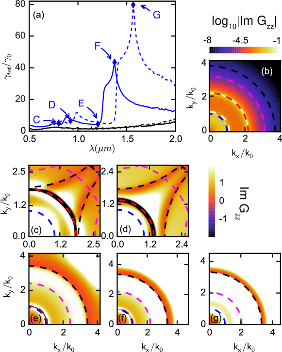
Figure 4: Emission rate of a dipole coupled to an aluminum sphere array embedded in a GaAs slab waveguide for an x-oriented dipole (black curves, left y-axis), and for a z-oriented dipole (blue curves, righthand y-axis). Solid (dashed) curves are for a lattice pitch of 145 (173) nm. (b) Contour plot of the integrand of a bare slab Green function $\log_{10}|Im[G_{zz}^{s}]|$. (c-g) Contour plot of $Im[G_{zz}]$, i.e., $\bar{\bm{I}}(\bm{k}_{||},\bm{r},\bm{r}_{0})$ in Eq. (10) for the special points, as marked by C,D, E, F, G in (a). In (b-g), the blue (black) dotted lines indicate the folded light line in air (GaAs), the white and magenta dotted lines for TE bound modes, the red dotted line for TM bound mode.

For many interesting quantities, plane wave calculations, together with the reciprocity technique suffice. These include angle-dependent extinction, absorption, reflection, refraction and diffraction and the differential radiated power for a localized source to any far field angle. However, for some highly interesting quantities, the array scanning method is indispensable. In general, a photonic structure may offer guided modes as efficient channels for emission, or in case of a plasmonic structure, may cause absorption. Generally, the total decay rate enhancement is due to the sum of induced quenching, emission into guided modes, and an increased rate of emission into far field modes. Only the last term is accessible to the reciprocity technique. The array scanning method, on the other hand, can be used to unravel quenching, and guided mode contributions. The full Brillouin zone integral in the array scanning method provides the sum of all three contributions, i.e., the full local density of states. In addition, as it gives the field at any position due to a localized source, one can calculate absorption. Finally, analyzing the integrand of Eq. (10) provides insight in the specific wave vectors that contribute to the local density of states, for instance pointing at guided mode contributions to the emission.

As third example to illustrate our method, we discuss a fluorescence problem tackled by the ASM method in which part of the emission enhancement of a dipole source is funneled into guided modes. As geometry we take a thin ($d=116nm$) layer of GaAs in air, and assume that a square lattice (lattice constant $p$) of aluminum particles (radius 0.25$p$) is embedded in the slab at about 2/3rds of the slab thickness (all dielectric constants taken from Palik Palik ). We assume a source located just above the slab top surface (25 nm separation). This geometry is not altogether realistic from an experimental stand point but has many illustrative challenges from a computational point of view. These are (A) as opposed to the previous examples the particles are inside a layer while the source is on top, (B) strong coupling of the particles to the slab waveguide mode, (C) no mirror symmetry in the geometry, so that particles couple to TE and TM modes, and (D) evanescent coupling of the source to the slab wave guide mode. We consider this computationally tough problem in a range of near- to mid-IR wavelengths, and for two pitches.

As shown in Fig. 4 (a), we study the total decay rate enhancement (in current literature often referred to as Purcell factor ($F$)) of a dipolar emitter, coupled to the scatterer/waveguide system. The total decay rate enhancement is given by the total emission rate $\gamma_{tot}$ divided by the vacuum rate $\gamma_{0}$. In Fig. 4 (a), results are shown for the emitter oriented in plane (along x-direction, black lines), and normal to the plane (along z-direction, blue lines). In this diagram solid lines refer to $p$=145 nm, while dashed lines refer to $p=$173 nm. For x-dipoles, the Purcell factor increases moderately, towards long wavelengths, which is due to increased material losses in aluminum particles at long wavelength. In contrast, the increase of the Purcell factor for a z-dipole coupled to the same configuration of lattice-waveguide system is pronounced, attaining values up to 40 or 80 for different pitches, as evident by the sharp peaks denoted by F (1.37 $\mu$m) and G (1.57 $\mu$m) in Fig. 4 (a). The large enhancement of $\gamma_{tot}$ results from the excitation of dark modes, i.e., guided modes, of the plasmonic lattice for long wavelengths, rather than merely from increased material losses. This is evident from two facts: (1) the peaks F, G are not close to the wavelength of maximum material losses, (2) the enhanced emission rate, up to 80, for z-dipoles far exceeds that for x-dipoles, which is less than 8.

To further study the dark mode excitation, we plot the integrands of the scattering part of the Green function, i.e., $\bar{\bm{I}}(\bm{k}_{||},\bm{r},\bm{r}_{0})$ in Eq. (10), in one quadrant of the full Brillouin zone in Fig. 4 (d-k) for special points C,D, E, F, G marked in Fig. 4 (a), in all cases focusing on the $z$-oriented dipole case. For reference, one can also evaluate the integrand for a ‘bare’ slab, containing a lattice of particles of zero polarizability, shown in Fig. 4 (b) at wavelength of 1 $\mu$m. In all panels, the plot range encompasses exactly the positive quadrant of the first Brillouin zone. In (b-h), blue (black) dotted lines indicate the light line in air (GaAs). Due to C₄ symmetry of the square lattice, the integrands in the full Brillouin zone can be obtained by mirroring along $k_{x}=0$, and $k_{y}=0$. In order to directly compare the k-space spectrum content, we use the same colormap for all contour plots in (c-g). The bare slab system supports three waveguides modes at short wavelength as shown in (b), i.e., two TE modes indicated by white and magenta dashed lines, plus one TM mode indicated by a red dashed line. At longer wavelength the fundamental TM /TE mode indicated by the magenta/red dotted line remains, while the higher order TE mode (white dotted line) vanishes.

In the bare slab waveguide in Fig. 4 (c), the contribution of the waveguide mode to the integrand of scattering part of Green function is weak, as shown in the contour plot of $\log_{10}|Im[G_{zz}]|$. For larger in-plane momentum, the integrand of the scattering part of Green function approaches 0. However, with the lattice of scatterers in place, the integrands of the second term in Eq. (10) are strongly mediated by the periodic scatterers. At short wavelengths, i.e., (c,d), there are three major features: (1) the bare slab waveguide supports well-defined waveguide modes, indicated by the dark arcs; (2) diffraction occurs, where the guided modes of the slab waveguide folds back into the Brillouin zone; (3) dark plasmonic modes are excited on the lattice in Fig. 4 (d-h) in a limited region of k-space close to the folded guided mode and is evident as very large integrand (bright features). At longer wavelengths (e-g), the dipole lattices become denser with respect to vacuum wavelength, so that back-folding no longer leads to intersections appearing with back-folded waveguide modes. Plasmon hybridization becomes stronger, and hence lattice resonances may play a significant role in the enhancement of $F$. Indeed, the integrand in Fig. 4 (e-g) shows that there are considerable plasmonic contributions (broad bright features) in the Brillouin zone within the (folded) light cone ( roughly 3.35$k_{0}$) given by GaAs, besides the narrow contribution from guided modes, which are only weakly confined at these long wavelengths. In Fig. 4 (d), a major part of the emission is inside the folded light cone given by the slab medium (GaAs), and includes a considerable amount inside the vacuum light cone ($k_{0}$), which indicates that a significant fraction of the total emission can be delivered into the far field. In contrast, one notices that in the integrand in Fig. 4 (e-g), the major contribution to $\gamma_{tot}$ lies outside the vacuum light cone. Hence, most of the emission is funneled into the dark modes of the lattice, and is eventually dissipated due to material losses.

The emission distribution in k-space, i.e., the fraction of the emission fuelled into far-field, as well as into the dark modes, for points C-G are tabulated in Table. (1). As evident in Fig. 4 (c-e), the the major contribution to the integrand appears at parallel wave vectors beyond the light-line of the host material of the lattice. The fraction of emission into the far field, i.e., $|\bm{k}_{||}|<k_{0}$, reaches its maximum value ($0.35\%$) at the point marked D. Further to the red, i.e, at point E, we see that emission with large parallel k-component, i.e., $|\bm{k}_{||}|\geq n_{GaAs}k_{0}$, starts to contribute due to the stronger plasmonic hybridization. As the wavelength increases further, the emission with $|\bm{k}_{||}|\geq n_{GaAs}k_{0}$ quickly dominates, which yields nearly $100\%$ emission funnelled into the dark mode of the plasmon lattice. Due to the large $|\bm{k}_{||}|$, those modes are tightly confined by the plasmonic lattice, and quickly dissipate due to material losses. It is important to realize that designing the k-space emission distribution is highly non-trivial, and the rules behind such type of design are beyond the scope of this paper. Essentially, it is the competition among channels, i.e., the emission with $|\bm{k}_{||}<k_{0}$, $k_{0}<|\bm{k}_{||}|\geq n_{GaAs}k_{0}$, and $|\bm{k}_{||}|\geq n_{GaAs}k_{0}$, that ultimately determines how emission occurs in the complex photonic environments ZhouLei2015PRL . Our method can aid evaluating different designs on basis of the fact that the integrand in the ASM method can be separated in different contributions. To conclude this example, the ASM-method provides key insights in the emission distribution in k-space, which could be utilized in many problems that require engineering the emission distribution in k-space as well as the separation of emission into far field, guided modes, and absorption.

	C	D	E	F	G
$\gamma_{tot}$	5.04	6.53	4.47	43.44	79.69
Fraction ($|\bm{k}_{||}|<k_{0}$ )	0.16	0.35	0.05	0.005	0.003
Fraction ($|\bm{k}_{||}|\geq n_{GaAs}k_{0}$)	0	0	0.14	0.92	0.95

Table 1: Fraction of emission of z-dipole coupled to waveguide-lattice system in k-space. C, D, E, F, G denote the special points marked in Fig. 4 (a).

IV Conclusion

In closing, we presented a general point dipole theory for periodic metasurfaces that are embedded in arbitrary stratified layer systems. With the assistance of Ewald’s summation technique and dyadic Green’s function of stratified layers, we study magnetoelectric scattering lattices coupled to layered photonic structures. One can with this method rapidly understand the physics of complicated structures by approximating meta-atoms as point dipoles with magnetoelectric responses, while accounting for all particle-particle interactions self-consistently via freely propagating photons as well as bound modes provided by the stratified layers. We further extended the plane wave excitation case to excitation by a single, localized, dipolar source, through the array scanning method. Thereby, all the relevant optical properties, such as LDOS and far field emission patterns, of the coupled waveguide lattice, can be extracted straightforwardly.

As applications of the proposed method, we demonstated that it applies readily to solid-state lighting scenarios where point emitters are coupled to periodic plasmonic lattices, in turn embedded in high index layered systems. Also, we applied our method to a plasmon enhanced thin-film solar cell structure containing a plasmonic nanoantenna array. We find that our method can efficiently handle such structures, capturing salient features due to diffractive coupling in terms of extinction, absorption and reflection. Due to high efficiency and flexibility of the dipole theory, it can be used for both diffractive, dilute lattices, and for dense lattices with complex clusters of inclusions that form a metamaterial or metasurface. We envision that our method is useful for studying metasurfaces, as well as related applications such as light-emitting diodes and solar cells.

V Acknowledgement

Y.T. Chen would like to thank Prof. S. A. Tretyakov for fruitful discussions. Y.T. Chen acknowledges financial support from the National Natural Science Foundation of China (Grant No. 61405067), and Foundation for Innovative Research Groups of the Natural Science Foundation of Hubei Province (Grant No. 2014CFA004). This work is part of the research program of the “Foundation for Fundamental Research on Matter (FOM)”, which is financially supported by the “The Netherlands Organization for Scientific Research (NWO)”. A.F.K. gratefully acknowledges an NWO-Vidi and Vici grant for financial support.

Appendix A Construction of free space dyadic Green’s function based on plane wave expansion

For a given wave vector $\bm{k}=[\bm{k}_{||},k_{z}]$, the TE and TM polarization modes associated with a plane wave are given by $\bm{E}_{TE}(\bm{r})=\bm{M}(\bm{k}_{||},\pm_{1},\pm_{2})e^{i\bm{k}_{||}\cdot\bm{r}_{||}}$, and $\bm{E}_{TM}(\bm{r})=\bm{N}(\bm{k}_{||},\pm_{1},\pm_{2})e^{i\bm{k}_{||}\cdot\bm{r}_{||}}$ respectively, where $\bm{M}$ and $\bm{N}$ are defined as follows,

$$\bm{M}(\bm{k}_{||,\pm_{1},\pm_{2}}) =e^{i\pm_{2}k_{z}z}\left(\hat{x}\frac{-k_{y}}{k_{||}}+\hat{y}\frac{k_{x}}{k_{||}}\right),$$ (14a)

$$\bm{N}(\bm{k}_{||,\pm_{1},\pm_{2}}) =e^{i\pm_{2}k_{z}z}\left[\hat{z}\frac{ik_{||}}{k_{0}}-\hat{x}\frac{i(\pm_{1})k_{z}k_{x}}{k_{||}k_{0}}-\hat{y}\frac{i(\pm_{1})k_{z}k_{y}}{k_{||}k_{0}}\right],$$ (14b)

where $\bm{r}=[\bm{r}_{||},z]$, $k_{||}=|\bm{k}_{||}|$, $k_{0}=\sqrt{k_{||}^{2}+k_{z}^{2}}$. The first sign factor describes the propagation direction along z-axis, while the second sign factor denotes the sign of $k_{z}$ in the construction of the basis function. Throughout the paper, we will use $\bm{M}(\bm{r},\pm,\pm)$ and $\bm{N}(\bm{r},\pm,\pm)$ for short. In the above formulation, the prefactors of TE and TM waves are arranged to fullfil the relation of

$$\begin{array}[]{c}\nabla\times[e^{i\bm{k}_{||}\cdot\bm{r}_{||}}M(\bm{k}_{||},\pm,\pm)]=e^{i\bm{k}_{||}\cdot\bm{r}_{||}}k_{0}N(\bm{k}_{||},\pm,\pm),\\ \nabla\times[e^{i\bm{k}_{||}\cdot\bm{r}_{||}}N(\bm{k}_{||},\pm,\pm)]=e^{i\bm{k}_{||}\cdot\bm{r}_{||}}k_{0}M(\bm{k}_{||},\pm,\pm).\end{array}$$ (15)

In free space, the dyadic Green function of the electric field can be expanded using the plane waves as follows (upper sign applies for $z>=z^{\prime}$),

$$\begin{aligned} \bar{\bm{G}}_{0}^{ee}(\bm{r},\bm{r}^{\prime})&=\frac{i}{8\pi^{2}}\int dk_{x}dk_{y}\frac{e^{i\theta}}{k_{z}}[\bm{M}_{+}\otimes\bm{M}^{\prime}_{-}-\bm{N}_{+}\otimes\bm{N}^{\prime}_{-}]\\ \bar{\bm{G}}_{0}^{he}(\bm{r},\bm{r}^{\prime})&=\frac{ik_{0}}{8\pi^{2}}\int dk_{x}dk_{y}\frac{e^{i\theta}}{k_{z}}[\bm{N}_{+}\otimes\bm{M}^{\prime}_{-}-\bm{M}_{+}\otimes\bm{N}^{\prime}_{-}],\\ \bar{\bm{G}}_{0}^{hh}(\bm{r},\bm{r}^{\prime})&=\frac{i}{8\pi^{2}}\int dk_{x}dk_{y}\frac{e^{i\theta}}{k_{z}}[-\bm{N}_{+}\otimes\bm{N}^{\prime}_{-}+\bm{M}_{+}\otimes\bm{M}^{\prime}_{-}],\\ \bar{\bm{G}}_{0}^{he}(\bm{r},\bm{r}^{\prime})&=\frac{ik_{0}}{8\pi^{2}}\int dk_{x}dk_{y}\frac{e^{i\theta}}{k_{z}}[-\bm{M}_{+}\otimes\bm{N}^{\prime}_{-}+\bm{N}_{+}\otimes\bm{M}^{\prime}_{-}].\end{aligned}$$ (16)

where $\theta=\bm{k}_{||}\cdot(\bm{r}_{||}-\bm{r}_{||}^{{}^{\prime}})$, $\bm{M}_{(\pm)}/\bm{N}_{(\pm)}=\bm{M}/\bm{N}(\bm{k}_{||},\pm,\pm)$, $\bm{M}^{\prime}_{(\mp)}/\bm{N}^{\prime}_{(\mp)}=\bm{M}/\bm{N}(\bm{k}_{||},\pm,\mp)$.

Appendix B Dyadic Green’s function for an interface

Dyadic Green function for an interface or stratified structure can be expanded using the plane waves, i.e., $\bar{\bm{G}}_{if}(\bm{r},\bm{r}^{\prime})=\bar{\bm{G}}_{0}(\bm{r},\bm{r}^{\prime})+\bar{\bm{G}}_{s}^{if}(\bm{r},\bm{r}^{\prime})$, where $\bar{\bm{G}}_{0}(\bm{r},\bm{r}^{\prime})$ is the free space terms given by Eq. (17).

$$\begin{aligned} \bar{\bm{G}}_{s,ee}^{if}&=\frac{i}{8\pi^{2}}\int d\bm{k}_{||}\frac{e^{i\theta}}{k_{z}}\{\gamma_{s}\bm{M}_{+}\otimes\bm{M}^{\prime}_{+}-\gamma_{p}\bm{N}_{+}\otimes\bm{N}^{\prime}_{+}\}\\ \bar{\bm{G}}_{s,he}^{if}&=\frac{ik_{0}}{8\pi^{2}}\int d\bm{k}_{||}\frac{e^{i\theta}}{k_{z}}\{\gamma_{s}\bm{N}_{+}\otimes\bm{M}^{\prime}_{+}-\gamma_{p}\bm{M}_{+}\otimes\bm{N}^{\prime}_{+}\},\\ \bar{\bm{G}}_{s,hh}^{if}&=\frac{i}{8\pi^{2}}\int d\bm{k}_{||}\frac{e^{i\theta}}{k_{z}}\{\gamma_{p}\bm{M}_{+}\otimes\bm{M}^{\prime}_{+}-\gamma_{s}\bm{N}_{+}\otimes\bm{N}^{\prime}_{+}\},\\ \bar{\bm{G}}_{s,eh}^{if}&=\frac{ik_{0}}{8\pi^{2}}\int d\bm{k}_{||}\frac{e^{i\theta}}{k_{z}}\{\gamma_{p}\bm{N}_{+}\otimes\bm{M}^{\prime}_{+}-\gamma_{s}\bm{M}_{+}\otimes\bm{N}^{\prime}_{+}\}.\end{aligned}$$ (17)

B.1 Dyadic Green function for an slab structure

Dyadic Green function for an slab structure can be expanded using the plane waves as follows KlimovPRA2005 ; HartmanJCP ; Cheng1986 , see the geometry in Fig. 1 (a), in which both the emitter and the detection point are located in the layer 2,

$$\begin{aligned} &\bar{\bm{G}}^{ee}_{{}_{2,2}}(\bm{r},\bm{r}^{\prime})=\int d\bm{k}_{||}\frac{ie^{i\theta}}{8\pi^{2}k_{z2}}\{\\ &\frac{1}{\Delta_{s}}[\bm{M}_{(+)}+\gamma_{s,21}(k_{||})\bm{M}_{(-)}\eta]\otimes[\bm{M}^{{}^{\prime}}_{(-)}+\gamma_{s,23}(k_{||})\bm{M}^{{}^{\prime}}_{(+)}]\\ &-\frac{1}{\Delta_{p}}[\bm{N}_{(+)}+\gamma_{p,21}(k_{||})\bm{N}_{(-)}\eta]\otimes[\bm{N}^{{}^{\prime}}_{(-)}+\gamma_{p,23}(k_{||})\bm{N}^{{}^{\prime}}_{(+)}]\},\\ &\bar{\bm{G}}^{he}_{{}_{2,2}}(\bm{r},\bm{r}^{\prime})=\int d\bm{k}_{||}\frac{ie^{i\theta}k_{0}}{8\pi^{2}k_{z2}}\{\\ &\frac{1}{\Delta_{s}}[\bm{N}_{(+)}+\gamma_{s,21}(k_{||})\bm{N}_{(-)}\eta]\otimes[\bm{M}^{{}^{\prime}}_{(-)}+\gamma_{s,23}(k_{||})\bm{M}^{{}^{\prime}}_{(+)}]\\ &-\frac{1}{\Delta_{p}}[\bm{M}_{(+)}+\gamma_{p,21}(k_{||})\bm{M}_{(-)}\eta]\otimes[\bm{N}^{{}^{\prime}}_{(-)}+\gamma_{p,23}(k_{||})\bm{N}^{{}^{\prime}}_{(+)}]\},\\ &\bar{\bm{G}}^{hh}_{{}_{2,2}}(\bm{r},\bm{r}^{\prime})=\int d\bm{k}_{||}\frac{ie^{i\theta}}{8\pi^{2}k_{z2}}\{\\ &\frac{1}{\Delta_{s}}[\bm{N}_{(+)}+\gamma_{s,21}(k_{||})\bm{N}_{(-)}\eta]\otimes[\bm{N}^{{}^{\prime}}_{(-)}+\gamma_{s,23}(k_{||})\bm{N}^{{}^{\prime}}_{(+)}]\\ &-\frac{1}{\Delta_{p}}[\bm{M}_{(+)}+\gamma_{p,21}(k_{||})\bm{M}_{(-)}\eta]\otimes[\bm{M}^{{}^{\prime}}_{(+)}+\gamma_{p,23}(k_{||})\bm{M}^{{}^{\prime}}_{(-)}]\},\\ &\bar{\bm{G}}^{eh}_{{}_{2,2}}(\bm{r},\bm{r}^{\prime})=\int d\bm{k}_{||}\frac{ie^{i\theta}k_{0}}{8\pi^{2}k_{z2}}\{\\ &\frac{1}{\Delta_{s}}[\bm{M}_{(+)}+\gamma_{s,21}(k_{||})\bm{M}_{(-)}\eta]\otimes[\bm{N}^{{}^{\prime}}_{(-)}+\gamma_{s,23}(k_{||})\bm{N}^{{}^{\prime}}_{(+)}]\\ &-\frac{1}{\Delta_{p}}[\bm{N}_{(+)}+\gamma_{p,21}(k_{||})\bm{N}_{(-)}\eta]\otimes[\bm{M}^{{}^{\prime}}_{(-)}+\gamma_{p,23}(k_{||})\bm{M}^{{}^{\prime}}_{(+)}]\}.\end{aligned}$$ (18)

where $\Delta_{s/p}=1-\gamma_{s/p,21}(k_{||})\gamma_{s/p,23}(k_{||})e^{i2k_{z}d}$, and $\gamma_{s,ij}=\frac{k_{zi}-k_{zj}}{k_{zi}+k_{zj}}$, $\gamma_{p,ij}=\frac{\epsilon_{j}k_{zi}-\epsilon_{i}k_{zj}}{k_{zi}\epsilon_{j}+k_{zj}\epsilon_{i}}$, $\eta=e^{i2k_{z}d}$.

References

- (1) Willets K A and van Duyne R P 2007 Annu. Rev. Phys. Chem. 58, 267.
- (2) Schnitzer I, Yablonovitch E, Caneau C, Gmitter T J and Scherer A 1993 Appl. Phys. Lett. 63, 2174.
- (3) Vuckovic J, Lončar M and Scherer A 2000 IEEE J. Quantum Electron., 36, 1131.
- (4) Okamoto K, Niki I, Shvartser A, Narukawa Y, Mukai A and A Scherer 2004 Nat. Mater., 3, 601.
- (5) Yeh D M, Huang C F, Chen C Y, Lu Y C and Yang C C 2008 Nanotechnology, PIER 19, 345201.
- (6) Henson J, DiMaria J, Dimakis E, Moustakas T D and Paiella R 2012 Opt. Lett. 37, 79.
- (7) Barnes W L 1999 J. Lightwave technol., 17, 2170.
- (8) Rigneault H, Lemarchand F, Sentenac A and Giovanini H 1999 Opt. Lett. 24, 148.
- (9) Lozano G Louwers D J, Rodriguez S R K, Murai S, Jansen O T A, Verschuuren M A and Gómez Rivas J 2013 Light Sci. Appl. 2, e66.
- (10) van Lare M, Lenzmann F, Verschuuren M A and Polman A 2012 Appl. Phys. Lett. 101, 221110.
- (11) Ferry V E, Verschuuren M A, Li H B T, Verhagen E, Walters R J, Schropp R E I, Atwater H A and Polman A 2010 Opt. Express, 18, A237.
- (12) Schokker A H and Koenderink A F 2014 Phys. Rev. B 90, 155452.
- (13) Auguié B and Barnes W L 2008 Phys. Rev. Lett. 101, 143902.
- (14) Törmä P and Barnes W L 2015 Rep. Prog. Phys. 78, 013901.
- (15) Kravets V G, Schedin F and Grigorenko A N 2008 Phys. Rev. Lett. 101, 087403.
- (16) Sersic I, Frimmer M, Verhagen E and Koenderink A F 2009 Phys. Rev. Lett. 103, 213902.
- (17) Gansel J K Thiel M Rill M S , Decker M , Bade K Saile V Freymann G V Linden S and Wegener M 2009 Science 325, 1513.
- (18) Yu N , Genevet P , Kats M A Aieta F , Tetienne J P , Capasso F and Gaburro Z 2011 Science, 334, 333.
- (19) Yu N , and Capasso F 2014 Nat. Mater., 13, 139.
- (20) Minovich A E Miroshnichenko A E , Bykov A Y , Murzina T V , Neshev D N and Kivshar Y S 2015 Laser Photon. Rev. 9, 195.
- (21) García Abajo F J, Sáenz J J, Campillo I and Dolado J S 2006 Opt. Express 14, 7.
- (22) Ra’di Y Simovski C R, and Tretyakov S A 2015 Phys. Rev. Appl. 3, 037001.
- (23) Landy N I, Sajuyigbe S, Mock J J, Smith D R and Padilla W J 2008 Phys. Rev. Lett. 100, 207402.
- (24) Fedotov V A, Mladyonov P L, Prosvirnin S L, Rogacheva A V, Chen Y and Zheludev N I 2006 Phys. Rev. Lett. 97, 167401.
- (25) Menzel C, Helgert C, Rockstuhl C, Kley E -B, Tünnermann A, Pertsch T and Lederer F 2010 Phys. Rev. Lett. 104, 253902.
- (26) David A, Benisty H and Weisbuch C 2012 Rep. Prog. Phys. 75, 126501.
- (27) Iida D, Fadil A, Chen Y T, Ou Y Y, Kopylov O, Iwaya M, Takeuchi T, Kamiyama S, Akasaki I and Ou H Y 2015 AIP Adv. 5, 097169.
- (28) Catchpole K R and Polman A 2008 Appl. Phys. Lett. 93, 191113.
- (29) Catchpole K R, and Polman A 2008 Opt. Express 16, 21793.
- (30) Fedotov V A, Wallauer J, Walther M, Perino M, Papasimakis N, and Zheludev N I 2015 arixv: 1502 01464.
- (31) Pors A and Bozhevolnyi S I 2010 Opt. Express 21, 27438.
- (32) Chen Y T, Nielsen T R, Gregersen N, Lodahl P and Mørk J 2010 Phys. Rev. B 81, 125431.
- (33) Chen Y T, Gregersen N, Nielsen T R, Mørk J and Lodahl P 2010 Opt. Express, 18, 12489.
- (34) Sersic I, Tuambilangana C, Kampfrath T and Koenderink A F 2011 Phys. Rev. B 83, 245102.
- (35) Xu J, Wu B B and Chen Y T 2015 Opt. Express 23, 11566.
- (36) Lunnemann P , Sersic I , and Koenderink A F 2013 Phys. Rev. B 88, 245109.
- (37) Kwadrin A and Koenderink A F 2013 Phys. Rev. B 87, 125123.
- (38) Kwadrin A, Osorio C I and Koenderink A F, 2015 submitted Preprint Arxiv:1505 02727.
- (39) Eroglu A and Lee J K 2007 Progress in Electromagnetic Research, PIER 77, 391.
- (40) Novotny L and Hecht B 2006 Principles of nano-optics, Cambridge University Press).
- (41) Klimov V V and Ducloy M 2005 Phys. Rev. A 72, 043809.
- (42) Hartman R L, Cohen S M and Leung P T 1999 J. Chem. Phys. 110, 2189.
- (43) Cheng D H S 1986 Electromagnetics 6, 171.
- (44) Urbach H P and Rikken G L J A 1998 Phys. Rev. A 57, 3913.
- (45) Jung J Søndergaard T Pedersen T G Pedersen K Larsen A N and Nielsen B B 2011 Phys. Rev. B 83, 085419.
- (46) de Vries P, Coevorden D V and Lagendijk A 1998 Rev. Mod. Phys. 70, 447.
- (47) Linton, C M 2010 SIAM ReV. 52, 630.
- (48) Capolino F, Jackson D R, Donald R W and Leopold B F 2007 IEEE Trans. Antennas Propagat. 55, 1644.
- (49) Janssen O T A, Wachters A J H and Urbach H P Opt. Express 18, 24522 2010.
- (50) Rodriguez S R K, Chen Y T, Steinbusch T P, Verschuuren M A, Koenderink A F and Gómez Rivas J 2014 Phys. Rev. B 90, 235406.
- (51) Alonso-González P , Albella P, Neubrech F, Huck C, Chen J, Golmar F, Casanova F, Hueso L E, Pucci A, Aizpurua J, and Hillenbrand R 2013 Phys. Rev. Lett. 110, 203902.
- (52) Zuloaga J and Nordlander P 2011 Nano. Lett. 11, 1280.
- (53) Palik E D 1985 Handbook of Optical Constants of Solids (New York: Academic).
- (54) Qu C, Ma S J, Hao J M, Qiu M, Li X, Xiao S Y, Miao Z Q, Dai N, He Q, Sun S L and Zhou L 2015 arXiv:1507.00929.