Asymptotic behavior of the node degrees in the ensemble average of adjacency matrix

Abstract

Various important and useful quantities or measures that characterize the topological network structure are usually investigated for a network, then they are averaged over the samples. In this paper, we propose an explicit representation by the beforehand averaged adjacency matrix over samples of growing networks as a new general framework for investigating the characteristic quantities. It is applied to some network models, and shows a good approximation of degree distribution asymptotically. In particular, our approach will be applicable through the numerical calculations instead of intractable theoretical analysises, when the time-course of degree is a monotone increasing function like power-law or logarithm.

I Introduction

Many social, technological, and biological networks belong to a common scale-free (SF) structure Barabasi99a which consists of many low degree nodes and a few high degree nodes called as hubs. The degree distribution follows a power-law, therefore an SF network has an extreme vulnerability against hub attacks Albert00 . In addition, these real networks are classified into assotative and disassortative networks Newman03a . For examples, typical social networks, e.g. coauthorships and actor collaborations, are assotative, while typical technological and biological networks, e.g. Internet, World-Wide-Web, protein-interaction, and food webs, are disassortative. In assotative networks, nodes with similar degrees tend to be connected, and thus positive degree-degree correlations appear. In disassotative networks, nodes with different degrees: low and high degrees tend to be connected, and thus negative degree-degree correlations appear.

Through the above findings in network science, superior network theories and efficient algorithms have been developed for analyzing network topology and dynamics Newman10 . However, studies for the cases with degree-degree correlations are not clear enough for successful analysises of topological structures and epidemics on networks except some percolation analysises. Recently, it has been numerically and theoretically found that an onion-like structure with positive degree-degree correlations gives the nearly optimal robustness against hub attacks in an SF network Herrmann11 ; Schneider11 ; Tanizawa12 .

On the other hand, the average behavior of stochastically generated network models or empirical data samples of real networks is discussed in many applications. Usually, some characteristic quantities such as degree distribution or clustering coefficient are investigated for a network, then their quantities are averaged over the samples of networks in which the existence of a generation rule (mechanism) of the networks is assumed. In this paper, we focus on the beforehand averaged network structure over samples, and calculate the degree distribution for several models of growing network with or without degree-degree correlations. This representation will give a general framework for numerically investigating the characteristic topological quantities in growing networks. Since our framework is supported by the interesting property of ordering that older nodes tend to have higher degrees in a randomly growing network Callaway01 , a wide range of application to growing networks can be expected.

II Representation by the ensemble average of adjacency matrix

We consider a set of growing networks in which a new node is added with probabilistic links to existing nodes in a network at each time step. To study the average behavior of the stochastic processes in many samples, we use the ensemble average of adjacency matrix defined as follows.

$$A(t)\stackrel{{\scriptstyle\rm def}}{{=}}\left(\begin{array}[]{ccccccccc}0&1&a_{13}&\ldots&a_{ij}&\ldots&a_{1i}&\ldots&a_{1n}\\ 1&0&a_{23}&\ldots&a_{2j}&\ldots&a_{2i}&\ldots&a_{2n}\\ a_{31}&a_{32}&0&\ldots&a_{3j}&\ldots&a_{3i}&\ldots&a_{3n}\\ \vdots&\vdots&\vdots&\ddots&\vdots&\vdots&\vdots&\vdots&\vdots\\ a_{j1}&a_{j2}&a_{3j}&\ldots&0&\ldots&a_{ji}&\ldots&a_{jn}\\ \vdots&\vdots&\vdots&\vdots&\vdots&\ddots&\vdots&\vdots&\vdots\\ a_{i1}&a_{i2}&\ldots&\ldots&a_{ij}&\ldots&0&\ldots&a_{in}\\ \vdots&\vdots&\vdots&\vdots&\vdots&\vdots&\vdots&\ddots&\vdots\\ a_{n1}&a_{n2}&\ldots&\ldots&\ldots&\ldots&a_{ni}&\ldots&0\\ \end{array}\right)$$

Here, without loss of generality, we set connected two nodes as the minimum initial configuration: $a_{11}=a_{22}=0$, $a_{12}=a_{21}=1$, and the degree $k_{1}(0)=k_{2}(0)=1$. Note that at each time step the matrix is expanding with the inverse $L$ shape of elements $a_{1n},a_{2n},\ldots,a_{n-1n}$, $0$, $a_{nn-1},\ldots,a_{n2},a_{n1}$ at the right-bottom corner. The diagonal element $a_{ii}$ is always $0$ due to no self-loop at each node $i$. Other elements are $0\leq a_{ij}\leq 1$, $i\neq j$, as the average number of links from $i$ to $j$ over the samples of networks. The value of each element is defined in order according to the passage of time. We assume that there are no adding links between existing nodes $i,j<n$ at any time $t=n-2$. Only links between selected old nodes and new node $n$ are added in a growing network.

In the sample-based description, the ensemble average of adjacency matrix is

$$A(t)=\frac{A^{(1)}(t)+A^{(2)}(t)+\ldots+A^{(k)}(t)+\ldots+A^{({\cal N}_{s})}(t)}{{\cal N}_{s}},$$

where $A^{(k)}(t)$ denotes an adjacency matrix of the $k$-th sample whose elements are $a_{ij}^{(k)}=1$ or $0$ corresponded to the connection or disconnection from $i$ to $j$, but $a_{ij}^{(k)}=0$ or undefined for $i,j>t+2$ because of the size $n=t+2$ at time $t$. ${\cal N}_{s}$ denotes the number of samples. We remark that an adjacency matrix is fundamental and important because it includes the necessary and sufficient information about a network structure and is useful for a mathematical treatment.

In this explicit representation of general framework, for each $i$-th node, $i=1,2,\ldots,n-1$, the (out-)degree is updated from time $t-1$ to $t$,

$$k_{i}(t)=k_{i}(t-1)+a_{in}.$$ (1)

The (out-)degree of $n$-th node added at time $t=n-2$ is defined by the sum of links from node $n$ to nodes $i$,

$$k_{n}(t)\stackrel{{\scriptstyle\rm def}}{{=}}\sum_{i=1}^{n-1}a_{ni}.$$ (2)

We should remark that the iterative calculations of Eqs. (1)(2) are equivalent to the averaged values over the samples after calculating the degrees for each sample of the networks at time $t$. With this equivalence in mind, we investigate the asymptotic behavior of $k_{i}(t)$ for a large $t$. We note that $k_{i}(t)$ is a monotone non-decreasing function of time $t$ because of $k_{i}(t)-k_{i}(t-1)=a_{in}\geq 0$ from Eq. (1) in growing networks.

III Asymptotic behavior of the node degrees

As examples, we apply the ensemble average of adjacency matrix to some network models. However, our approach is applicable to other growing networks especially in a wide class, e.g. with approximately power-law or exponential degree distribution. In the following, we assume that each link is undirected: $a_{ij}=a_{ji}$.

III.1 Babarási and Albert model

Since the continuous-time approximation of Eq.(1) is generally

$$\frac{dk_{i}(t)}{dt}=a_{in},$$

our approach is applicable to the Babarási and Albert (BA) model Barabasi99b as follow.

preferential attachment:

$$a_{ni}=\frac{m\times k_{i}(t-1)}{\sum_{l}k_{l}(t-1)}\approx\frac{k_{i}(t-1)}{2t},$$

uniform attachment:

$$\forall i\;\;\;a_{ni}=\frac{m}{m_{0}+t-1},$$

where $m_{0}$ denotes the initial number of nodes, and $m$ denotes the number of adding links at each time step.

For the two cases of preferential and uniform attachments, $k_{i}(t)=m\sqrt{t/t_{i}}$ and $k_{i}(t)=m(\log(m_{0}+t-1)-\log(m_{0}+t_{i}-1)+1)$ have been derived with the corresponding degree distributions $p(k)\sim k^{-3}$ and $p(k)\sim e^{-k}$, respectively Barabasi99b . The analysis in BA model is based on the invariant ordering property of degrees in which older nodes get more links averagely at any time in the growth of network. Under the invariant ordering property, our approach can be regarded as an extension of mathematical treatment in the BA model through the representation by the ensemble average of adjacency matrix over samples of growing networks.

III.2 Duplication-divergence model

We preliminary introduce a duplication-divergence (D-D) model Satorras03 ; Sole02 without mutations of random links between existing nodes, whose generation mechanism is known as fundamental in biological protein-protein interaction networks. In the D-D model, at each time step, a new node is added and links to neighbor nodes of a uniformly randomly chosen node (see Figure 1(a)). Some duplication links are deleted with probability $\delta>0$. Here, no mutations are to simplify the discussion and to connect to the next subsection. Although the degree distribution in the D-D model can be approximately analyzed by the approach of mean-field-rate equation Satorras03 ; Sole02 , we show the applicability of our approach to the D-D model in order to extend it to more general networks. Moreover, in the next section, we reveal that older nodes tend to have higher degrees Callaway01 in the D-D model, whose ordering of degree $k_{i}(t)$ for node index $i$ was not found from the above approach.

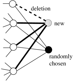
(a) D-D model

(b) Copying model

Figure 1: Basic linking processes at each time step from a new node to a randomly chosen node and/or the neighbor nodes in the growing networks. The thick bold lines show adding links, and the dashed line shows a deleted one. The thin lines show already existing links at that time.

Since the $n$-th new node links to the neighbor node $i$ of a chosen node $j\neq i$ from existing nodes $1\leq i,j\leq n-1$ in a network of D-D model, we have

$$a_{ni}=\frac{(1-\delta)\sum_{j=1}^{n-1}a_{ji}}{n-1}=\frac{1}{n-1}(1-\delta)k_{i}(t-1),$$ (3)

where we use the uniform selection probability $1/(n-1)$ of each node $j$ and the no-deletion rate $1-\delta$ for linking to the neighbor nodes.

From Eqs. (1)(2) (3), we obtain

$$k_{i}(t)=\left(1+\frac{1-\delta}{n-1}\right)k_{i}(t-1),$$ (4)

$$k_{n}(t)=\frac{1-\delta}{n-1}\sum_{i=1}^{n-1}k_{i}(t-1).$$ (5)

By applying Eq. (4) recursively, we derive

$$k_{i}(t) = \left(\frac{n-1+(1-\delta)}{n-1}\right)\left(\frac{n-2+(1-\delta)}{n-2}\right)\ldots\left(\frac{i+(1-\delta)}{i}\right)k_{i}$$

$$= \frac{\Gamma(n+(1-\delta))/\Gamma(i+(1-\delta))}{\Gamma(n)/\Gamma(i)}k_{i}\sim(t+1)^{1-\delta}.$$

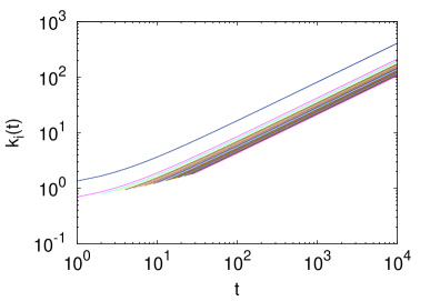
(a) $\delta=0.3$

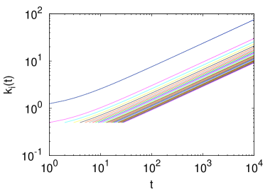
(b) $\delta=0.5$

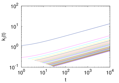
(c) $\delta=0.7$

Figure 2: Parallel curves of time-course $k_{i}(t)$ of degree in the D-D model with a rate $\delta$ of link deletion. The color lines from top to bottom correspond to the nodes $i=1$ or $2,3,4,\ldots,30$. Note that each node $i$ is born at time $t_{i}=i-2$.

In addition, the continuous-time approximation of Eq. (4) is

$$\frac{dk_{i}(t)}{dt}=a_{ni}=\frac{1-\delta}{t+1}k_{i}(t).$$

From the separation of variables method, we obtain the solution

$$k_{i}(t)=(t+1)^{1-\delta}\sim t^{1-\delta}.$$

When we denote the initial degree $k_{i}$ at the inserted time $t_{i}$ for a node $i$, the above solution is rewritten as

$$k_{i}(t)\approx k_{i}\left(\frac{t}{t_{i}}\right)^{1-\delta}.$$

From the existence of parallel curves shown in Fig. 2, the ordering of degrees

$$k_{n}(t)<k_{n-1}(t)<\ldots<k_{3}(t)<k_{2}(t)=k_{1}(t),$$ (6)

is not changed. In other word, older nodes get more links averagely. Thus, we obtain

$$p(k_{i}(t)<k)=p\left(t_{i}>\left(\frac{k_{i}}{k}\right)^{1/(1-\delta)}t\right)=\left(1-\frac{k_{i}^{1/(1-\delta)}}{k^{1/(1-\delta)}}\right)\frac{t}{N_{0}+t},$$

$$p(k)=\frac{\partial p(k_{i}(t)<k)}{\partial k}\sim k^{-(1+\frac{1}{1-\delta})},$$ (7)

where $N_{0}+t$ is the number of nodes at time $t$, and $N_{0}$ denotes the initial number of nodes. In the tail of degree distribution, the exponent of power-law is $1+\frac{1}{1-\delta}$ asymptotically. Note that the slightly different exponent $1+\frac{1}{1-\delta}$ to the conventional approximation Kim02 ; Satorras03 is not strange, since the mutations are necessary for their D-D models.

Figure 3(a)-(c) shows the time-course of $k_{i}(t)\sim t^{1-\delta}$ in the case of $\delta=0.3$, $0.5$, and $0.7$, respectively, averaged over $100$ samples. The black, orange, and magenta lines are the numerical results of Eqs. (4)(5) for the node $i=1$, $10$, and $100$. The cyan line guides the estimated slope of $1-\delta$ in log-log plot. In Fig. 3(d), the red, green, and blue lines show the degree distributions for $\delta=0.3$, $0.5$, and $0.7$, respectively, at the size $n=10^{4}$. The magenta, cyan, and gray dashed lines guides the corresponding slopes of $1+\frac{1}{1-\delta}$ for these $\delta$.

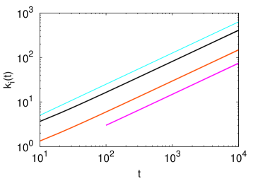
(a) $\delta=0.3$

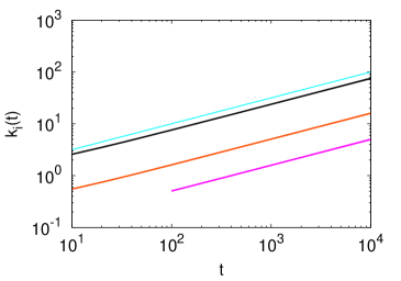
(b) $\delta=0.5$

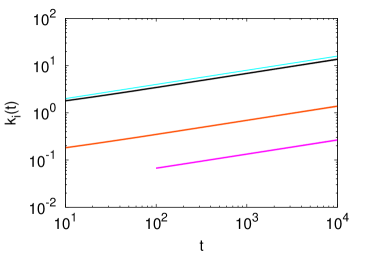
(c) $\delta=0.7$

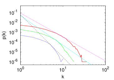
(d) $p(k)$

Figure 3: Results for the D-D model without mutations. (a)-(c) Time-courses $k_{i}(t)$ of degree for node $i=1,10,$ and $100$ shown by black, orange, and magenta lines, respectively, at the typical values of rate $\delta$ of link deletion. The cyan line guides the estimated slope $1-\delta$ of $k_{i}(t)\sim t^{1-\delta}$. (d) Degree distribution $p(k)$ in the cases of $\delta=0.3,0.5$, and $0.7$ shown by red, green, and blue lines, respectively. The dotted magenta, cyan, and gray lines show the estimated power-law distributions $k^{-\left(1+\frac{1}{1-\delta}\right)}$.

III.3 Copying model

A modification Hayashi14 of the D-D model Satorras03 ; Sole02 by adding a mutual link between a new node and a randomly chosen node has been proposed. The mutual link contributes to avoid the singularity called as non-self-averaging even for $\delta<1/2$ without mutations Hayashi14 . The growing network is constructed as shown in Fig. 1(b). It is referred to as copying model. At each time step, a new node is added. The new node links to a uniformly randomly chosen node, and to its neighbor nodes with probability $1-\delta$.

In the copying model, we have

$$a_{ni}=\frac{1+(1-\delta)\sum_{j=1}^{n-1}a_{ji}}{n-1}=\frac{1+(1-\delta)k_{i}(t-1)}{n-1},$$ (8)

since the $n$-th new node links to a uniformly randomly chosen node $i$ and to the neighbor node $i$ when other node $j$ is chosen from existing nodes $1\leq i,j\leq n-1$ in the network. These effects are in the first term $1/(n-1)$ and the second term $(1-\delta)\sum_{j=1}^{n-1}a_{ji}/(n-1)$ in Eq. (8).

From Eqs. (1)(2) (8), we obtain

$$k_{i}(t)=\frac{1}{n-1}+\left(1+\frac{1-\delta}{n-1}\right)k_{i}(t-1),$$ (9)

$$k_{n}(t)=1+\frac{1-\delta}{n-1}\sum_{i=1}^{n-1}k_{i}(t-1).$$ (10)

By applying Eq. (9) recursively, we derive

$$k_{i}(t) = \frac{1}{t+1}+\left(\frac{t+1+(1-\delta)}{t+1}\right)\left(\frac{1}{t}+\left(\frac{t+(1-\delta)}{t}k_{i}(t-2)\right)\right)$$ (11)

$$= \frac{1}{t+1}+\frac{t+1+(1-\delta)}{(t+1)t}+\ldots+\frac{\Gamma(t+2+(1-\delta))/\Gamma(i)}{\Gamma(t+2)/\Gamma(i)}k_{i}(t_{i})$$

$$\approx O(1/t)+(t+1)^{1-\delta},$$

where we use $n-1=t+1$ and the Staring formula $\Gamma(x+1)\approx x^{x}e^{-x}$.

In particular, by the mathematical induction, we confirm that the case of $\delta=0$ generates a sequence of the complete graphs with $k_{i}(t)=t+1=n-1$ links at every node of $i=1,2,\ldots,n$. First, $k_{1}(1)=k_{2}(1)=2$ and $k_{3}(1)=2$ are obvious. Next, we assume $k_{i}(t-1)=(t-1)+1=n-2$, from Eqs.(9)(10) we derive

$$k_{i}(t) = \frac{1}{n-1}+\left(1+\frac{1}{n-1}\right)(n-2)=\frac{1+(n-1)(n-2)+(n-2)}{n-1}$$

$$= \frac{(n-1)^{2}}{n-1}=n-1,$$

$$k_{n}(t)=1+\frac{(n-1)(n-2)}{n-1}=n-1.$$

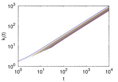
(a) $\delta=0.3$

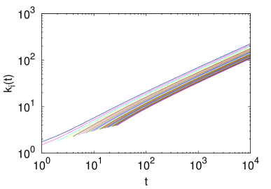
(b) $\delta=0.5$

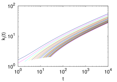
(c) $\delta=0.7$

Figure 4: Parallel curves of time-course $k_{i}(t)$ of degree in the copying model with a rate $\delta$ of link deletion. The color lines from top to bottom correspond to the nodes $i=1$ or $2,3,4,\ldots,30$. Note that each node $i$ is born at time $t_{i}=i-2$.

On the other hand, the continuous-time approximation of Eq.(9) is

$$\frac{dk_{i}(t)}{dt}=a_{ni}=\frac{1}{t+1}+\left(\frac{1-\delta}{t+1}\right)k_{i}(t).$$

Since this form is a 1st order linear differential equation $dk_{i}/dt+f(t)k_{i}=g(t)$, by applying the solution $e^{-\int f(t)dt}\left(e^{\int f(t)dt}g(t)dt+A\right)$, we obtain

$$k_{i}(t)=(t+1)^{1-\delta}\left(\int_{0}^{t}\frac{1}{(t+1)^{1+(1-\delta)}}dt+A\right)=A(t+1)^{1-\delta}-C^{\prime}\sim t^{1-\delta},$$

where $A$ and $C^{\prime}$ are constants of integration, and we use $f(t)\stackrel{{\scriptstyle\rm def}}{{=}}-(1-\delta)/(t+1)$ and $g(t)\stackrel{{\scriptstyle\rm def}}{{=}}1/(t+1)$. Note that the solution $t^{1-\delta}$ is only different by $O(1/t)$ to Eq.(11), and can be ignored for a large $t$. As similar to the D-D model in subsection 3.2, from Eq. (7) under the invariant ordering (6) in the parallel curves shown as Fig. 4, the degree distribution asymptotically follows a power-law with the exponent $1+\frac{1}{1-\delta}$.

Figure 5(a)-(c) shows the time-course of $k_{i}(t)\sim t^{1-\delta}$ in the cases of $\delta=0.3$, $0.5$, and $0.7$, respectively, averaged over $100$ samples. The black, orange, and magenta lines are the numerical results of Eqs. (9)(10) for the node $i=1$, $10$, and $100$. The cyan line guides the estimated slope of $1-\delta$ in log-log plot. It fits to the lines of $k_{i}(t)$ for a large $t$. Moreover, as shown in Fig. 5(d), Eq. (7) gives a good approximation at the size $n=10^{4}$. The red, green, and blue lines show the degree distributions for $\delta=0.3$, $0.5$, and $0.7$, respectively. The magenta, cyan, and gray dashed lines guides the corresponding slopes of $1+\frac{1}{1-\delta}$ for these $\delta$ in the fitting to the tails.

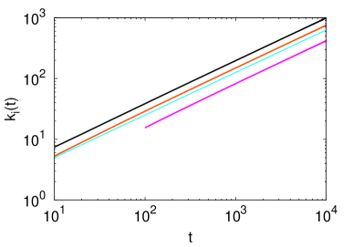
(a) $\delta=0.3$

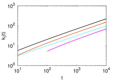
(b) $\delta=0.5$

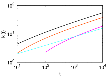
(c) $\delta=0.7$

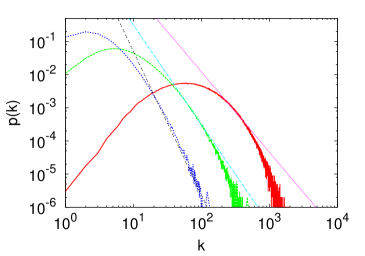
(d) $p(k)$

Figure 5: Results for the copying model. (a)-(c) Time-courses $k_{i}(t)$ of degree for node $i=1,10,$ and $100$ shown by black, orange, and magenta lines, respectively, at the typical values of rate $\delta$ of link deletion. The cyan line guides the estimated slope $1-\delta$ of $k_{i}(t)\sim t^{1-\delta}$. (d) Degree distribution $p(k)$ in the cases of $\delta=0.3,0.5$, and $0.7$ shown by red, green, and blue lines, respectively. The dotted magenta, cyan, and gray lines show the estimated power-law distributions $k^{-\left(1+\frac{1}{1-\delta}\right)}$.

III.4 Copying model with positive degree-degree correlations

In this subsection, we emphasize that our approach is effective through the numerical estimation, even when an analytic derivation is intractable.

We consider a copying model with positive degree-degree correlations based on a cooperative generation mechanism by linking homophily, in which densely connected cores among high degree nodes emerge Hayashi14 . In more detail, the difference to the previously mentioned copying model is that the $n$-th new node links to the neighbor nodes $j$ of a randomly chosen node $i$ with a probability $(1-\delta)f((1-\delta)k_{i}(t-1),k_{j}(t-1))$ from existing nodes in the network. Such a function

$$f(x,y)\stackrel{{\scriptstyle\rm def}}{{=}}\frac{1}{1+a|x-y|},$$

is necessary to enhance the degree-degree correlations, and $a>0$ is a parameter Wu11 . Since the degree of new node is unknown in advance due to the stochastic process, it is temporary set as $(1-\delta)k_{i}(t-1)$.

Thus, instead of Eq. (8), we substitute

$$a_{ni}\stackrel{{\scriptstyle\rm def}}{{=}}\frac{1+(1-\delta)\sum_{j=1}^{n-1}a_{ji}\times f((1-\delta)k_{i}(t-1),k_{j}(t-1))}{n-1},$$ (12)

for Eqs. (1)(2).

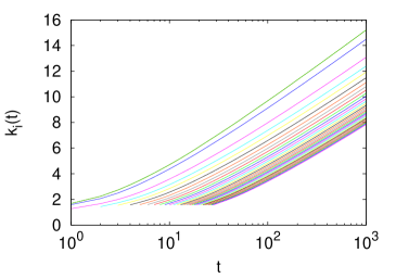
(a) $\delta=0.3$

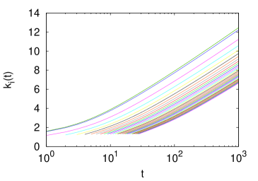
(b) $\delta=0.5$

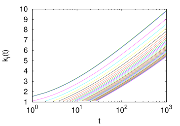
(c) $\delta=0.7$

Figure 6: Parallel curves of time-course $k_{i}(t)$ of degree in the copying model with positive degree-degree correlations and a rate $\delta$ of link deletion. The color lines from top to bottom correspond to the nodes $i=1$ or $2,3,4,\ldots,30$. Note that each node $i$ is born at time $t_{i}=i-2$.

Although the theoretical analysis of Eqs. (1)(2) for Eq. (12) is difficult, the iterative calculations are possible numerically. When we assume $\beta k_{i}(t)\sim\log(t)$, we derive an exponential distribution as follows. From $t\sim e^{\beta k_{i}(t)}$, we obtain

$$\frac{t_{i}}{t}=\frac{e^{\beta k_{i}}}{e^{\beta k_{i}(t)}},$$

$$p(k_{i}(t)<k)=p(t_{i}>\frac{e^{\beta k_{i}}}{e^{\beta k}}t)=\left(1-\frac{e^{\beta k_{i}}}{e^{\beta k}}\right)\frac{t}{N_{0}+t},$$

$$p(k)=\frac{\partial p(k_{i}(t)<k)}{\partial k}\sim e^{-\beta k},$$

under the invariant ordering (6) in the parallel curves shown as Fig. 6.

Figure 7(a)-(c) shows that $k_{i}(t)$ denoted by black, orange, and magenta lines for $i=1$, $10$, and $100$ is approximated by $\log(t)$ in the copying model with degree-degree correlations. The cyan lines guide the estimated slopes $\beta=2.222$, $1.818$, and $1.428$ for $\delta=0.3$, $0.5$, and $0.7$, respectively, in the numerical fittings for the iterative calculations of Eqs. (1)(2)(12). Thus, as shown in Fig. 7(d), the tails in $p(k)$ denoted by red, green, and blue lines for $\delta=0.3$, $0.5$, and $0.7$ are approximated by $e^{-\beta k}$ shown as magenta, cyan, and gray dashed lines at the size $n=10^{3}$. Note that $p(k)$ is only slightly deviated but the exponential part is remained by adding shortcut links in order to self-organize a robust onion-like structure in the incrementally growing network Hayashi14 .

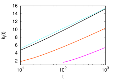
(a) $\delta=0.3$

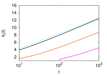
(b) $\delta=0.5$

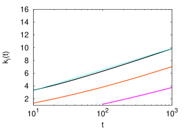
(c) $\delta=0.7$

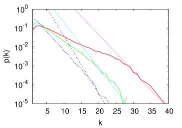
(d) $p(k)$

Figure 7: Results for the copying model with positive degree-degree correlations. (a)-(c) Time-courses $k_{i}(t)$ of degree for node $i=1,10,$ and $100$ shown by black, orange, and magenta lines, respectively, at the typical values of rate $\delta$ of link deletion. The cyan line guides the estimated slope $1/\beta$ of $k_{i}(t)\sim\log(t)/\beta$ in semi-log plot. (d) Degree distribution $p(k)$ in the cases of $\delta=0.3,0.5$, and $0.7$ shown by red, green, and blue lines, respectively. The dotted magenta, cyan, and gray lines show the estimated exponential distributions $e^{-\beta k}$.

III.5 More general case

We consider the asymptotic behavior of the node degrees for a general case in growing networks. When the time-course $k_{i}(t)$ of degree follows a monotone increasing function $g(t)$ of time $t$, there exists the inverse function $h(k)\stackrel{{\scriptstyle\rm def}}{{=}}g^{-1}(k)=t$. It is possible that the time-course $k_{i}(t)$ is an average of observed real data for node $i$, e.g. born at time $t-2$. From

$$\frac{t_{i}}{t}=\frac{h(k_{i})}{h(k)},$$

we have

$$p(k_{i}(t)<k)=p\left(t_{i}>\frac{h(k_{i})}{h(k)}t\right).$$

Then, on the assumption of the invariant ordering (6) in parallel curves of $\{k_{i}(t)\}$, we derive

$$p(k)=\frac{\partial p(k_{i}(t)<k)}{\partial k}=\frac{\partial}{\partial k}\left(1-\frac{{\rm const.}}{h(k)}\right)\frac{t}{N_{0}+t}\sim\frac{h^{\prime}(k)}{h^{2}(k)}.$$

where $h^{\prime}(k)$ denote the derivative of $h(k)$ by the variable $k$. We should remark that various degree distributions of non-power-law may appear depending on the shape of monotone increasing function $k_{i}(t)$ according to what type of generation in growing networks.

IV Analytic deviation for the invariant ordering of node degrees

We derive the invariant ordering (6) at any time $t$ within parallel curves of monotone increasing functions for the D-D and copying models discussed in subsections 3.2 and 3.3. In the following, we use double mathematical induction for node index $i$ and time $t$.

Once $k_{i}(t-1)-k_{j}(t-1)>0$ is satisfied for $1$ or $2\leq i<j\leq n-1$ at $t=n-2\geq 1$,

$$k_{i}(t)-k_{j}(t) = (k_{i}(t-1)-k_{j}(t-1))+(a_{in}-a_{jn})$$ (13)

$$= \left(1+\frac{1-\delta}{n-1}\right)(k_{i}(t-1)-k_{j}(t-1))>0,$$

is obtained from Eqs. (1)(4)(9). Here, from Eqs. (4)(5) at $n=3$ with the initial condition $k_{1}(0)=k_{2}(0)=1$, we obtain

$$k_{1}(1)=k_{2}(1)=1+\frac{1-\delta}{2},\;\;\;k_{3}(1)=1-\delta<k_{1}(1)=k_{2}(1).$$

From Eqs. (9)(10) at $n=3$ with the same initial condition, we also obtain

$$k_{1}(1)=k_{2}(1)=2-\frac{\delta}{2},\;\;\;k_{3}(1)=1+\frac{1-\delta}{2}(1+1)<k_{1}(1)=k_{2}(1).$$

Since the assumption in Eq. (13) is satisfied for $i=1$ or $2$ and $j=3$ at $t=2$, we have

$$k_{3}(2) < k_{2}(2)=k_{1}(2),$$

$$\vdots$$

$$k_{3}(t) < k_{2}(t)=k_{1}(t),$$ (14)

by applying Eq. (13) recursively for $t\geq 2$.

On the other hand, from Eqs. (4)(5), we rewrite

$$k_{n}(t)=\frac{1-\delta}{n-1}\left(\sum_{i=1}^{n-2}k_{i}(t-1)+k_{n-1}(t-1)\right),$$

$$k_{n-1}(t)=\left(1+\frac{1-\delta}{n-1}\right)k_{n-1}(t-1),$$

$$k_{n-1}(t-1)=\frac{1-\delta}{n-2}\sum_{i=1}^{n-2}k_{i}(t-2),$$

at $t=n-2$, and

$$k_{i}(t-1)=\left(1+\frac{1-\delta}{n-2}\right)k_{i}(t-2),$$

for $i=1,2,\ldots,n-2$. Then, we have

$$k_{n-1}(t)-k_{n}(t)=\frac{1-\delta}{n-2}\left(1-\frac{n-1-\delta}{n-1}\right)\sum_{i=1}^{n-2}k_{i}(t-2)>0.$$ (15)

Similarly, from Eqs. (9)(10), we rewrite

$$k_{n}(t)=1+\frac{1-\delta}{n-1}\left(\sum_{i=1}^{n-2}k_{i}(t-1)+k_{n-1}(t-1)\right),$$

$$k_{n-1}(t)=\frac{1}{n-1}+\left(1+\frac{1-\delta}{n-1}\right)k_{n-1}(t-1),$$

$$k_{n-1}(t-1)=1+\frac{1-\delta}{n-2}\sum_{i=1}^{n-2}k_{i}(t-2),$$

at $t=n-2$, and

$$k_{i}(t-1)=\frac{1}{n-2}+\left(1+\frac{1-\delta}{n-2}\right)k_{i}(t-2),$$

for $i=1,2,\ldots,n-2$. Then, we also have

$$k_{n-1}(t)-k_{n}(t)=\frac{\delta}{n-1}+\frac{1-\delta}{n-2}\left(1-\frac{n-1-\delta}{n-1}\right)\sum_{i=1}^{n-2}k_{i}(t-2)>0.$$ (16)

By applying (13) recursively for $t>n-2$ after substituting Eq. (15) or (16) to the right-hand side of Eq. (13), we obtain

$$k_{3}(t)-k_{4}(t) > 0,$$

$$k_{4}(t)-k_{5}(t) > 0,$$

$$\vdots$$

$$k_{n-1}(t)-k_{n}(t) > 0.$$ (17)

From Eqs. (14)(17), we obtain the ordering (6) after all.

Next, we consider the existing condition of the ordering (6) within parallel curves of $\{k_{i}(t)\}$ for a general case of growing networks discussed in subsection 3.5.

From Eq. (1) for $1$ or $2\leq i<j\leq n-1$ at $t=n-2\geq 2$, we have

$$k_{i}(t)-k_{j}(t)=(k_{i}(t-1)-k_{j}(t-1))+(a_{in}-a_{jn}).$$ (18)

If older nodes tend to get more links,

$$a_{in}>a_{jn}$$ (19)

hold in the ensemble average of adjacency matrix. Then, we remark $k_{3}(t)<k_{2}(t)=k_{1}(t)$ from Eq. (19) and $k_{3}(1)=k_{3}(0)+a_{13}+a_{23}<k_{1}(1)=k_{1}(0)+a_{31}$ or $k_{2}(1)=k_{2}(0)+a_{32}$ with the initial values $k_{3}(0)=0$ and $k_{1}(0)=k_{2}(0)=1$.

On the other hand, from Eqs. (1)(2), we derive

$$k_{n-1}(t)-k_{n}(t)=\sum_{l=1}^{n-2}(a_{(n-1)l}-a_{nl}).$$

If Eq. (19) hold with $a_{ij}=a_{ji}$, for $n\geq 4$ we have

$$k_{n-1}(t)-k_{n}(t)>0.$$ (20)

Therefore, on the condition (19), we obtain the ordering (6) from Eqs. (18)(20).

V Conclusion

We have proposed the explicit representation by the ensemble average of adjacency matrix over samples of growing networks. The important point is that the adjacency matrix is averaged in advance before calculating a characteristic quantity about the topological structure for each sample. The ensemble average has been applied to some network models: BA Barabasi99b , D-D Satorras03 ; Sole02 , and copying Hayashi14 models for investigating the degree distributions in the asymptotic behavior by using the theoretical and numerical analysises for difference equations and the corresponding continuous-time approximation of differential equations with variables $t$ and $k_{i}(t)$. We have derived $k_{i}(t)\sim t^{1-\delta}$ and $p(k)\sim k^{-(1+\frac{1}{1-\delta})}$ for the D-D and copying models under the invariant ordering of degrees which is supported in randomly grown networks Callaway01 . Moreover, for the copying model with positive degree-degree correlations, we have shown that the numerical calculations of the difference equation give a good approximation of an estimated exponential distribution, even when an analytic derivation is intractable. The copying model with positive degree-degree correlations is related to the self-organization Hayashi14 of robust onion-like networks Herrmann11 ; Schneider11 ; Tanizawa12 .

Our approach may be also applicable to data analysis for social networks, when the observed time-course of degree is a monotone increasing function like power-law or logarithm in the average over samples by ignoring short-time fluctuations, and a node index $i$ or $j$ represents an ordering of its birth time. This expectation is supported as follows. It is helpful for grasping a trend to study the average behavior of many users (nodes) added at a same (sampling interval) time into a network community. Random growth in a social network probably corresponds to encountered chances among people. Moreover, as time goes by, the number of his/her friends for a member of social networks is usually increasing. It is natural that the connections to friends are maintained. However, we must consider the effect of rewirings between old members in the definition of adjacency matrix. Also from a practical viewpoint, $O(n^{2})$ space to store an adjacency matrix may cause a problem for dig data.

From the conventional analysis for special network models to a general framework, the representation by the ensemble average will open a door for investigating the characteristic quantities, e.g. node degrees in growing networks. In particular, the time-course of a quantity depending on the birth time of node is considered as a key point. The discussion about other quantities such as clustering coefficient or the number of paths of a given length requires further studies of how to analyze the average behavior related to the transitivity.

References

- (1) Albert, R., Jeong, H. and Babarási, A.-L. Error and attack tolerance of complex networks. Nature 406: pp.36–44, (2000).
- (2) Babarási, A.-L. and Albert, R. Emergence of scaling in random networks. Science 286: pp.509–512, (1999).
- (3) Babarási, A.-L., Albert, R. and Jeong, H. Mean-field theory for scale-free random networks. Physica A 272: pp.173–187, (1999).
- (4) Callaway, D.S., Hopcroft, J.E., Kleinberg, J.M., Newman, M.E.J. and Strogatz, S.H. Are randomly grown graphs really random ?. Physical Review E 64: pp.041902, (2001).
- (5) Hayashi, Y. Growing Self-organized Design of Efficient and Robust Complex Networks. IEEE Xplore Digital Library http://dx.doi.org/10.1109/SASO2014.17, Proc. of 2014 IEEE 8th Int. Conf. on SASO: Self-Adaptive and Self-Organizing Systems 2014, pp.50–59. arXiv:physics/1411.7719, (2014).
- (6) Herrmann, H.J., Schneider, C.M., Moreira, A.A., Andrade Jr. J.S., and Havlin, S. Onion-like network topology enhances robustness against malicious attacks. Journal of Statistical Mechanics P01027, (2011).
- (7) Kim, J., Krapivsky, P.L. and Redner, S. Infinite-order percolation and giant fluctuations in a protein interaction networks. Physical Review E 66: pp.055101(R), (2002).
- (8) Newman, M.E.J. Assortative Mixing in Networks. Physical Review Letters 89(20): pp.208701, (2003).
- (9) Newman, M.E.J. Networks -An Introduction. Oxford University Press, (2010).
- (10) Pastor-Satorras, R., Smith, E. and Sole, R.V. Evolving protein interaction networks through gene duplication. Journal of Theoretical Biology 222(2): pp.199–210, (2003).
- (11) Schneider, C.M., Moreira, A.A., Andrade Jr. J.S., Havlin, S. and Herrmann, H.J. Mitigation of malicious attacks on networks. Proceedings of the National Academy of Sciences of the United States of America 810(10): pp.3838–3841, (2011).
- (12) Sole, R.V., Pastor-Satorras, R., Smith, E. and Kepler, T.B. A model of large-scale proteome evolution. Advances in Complex Systems 5(1): pp.43–54, (2002).
- (13) Tanizawa, T., Havlin, S. and Stanley, H.E. Robustness of onionlike correlated networks against targeted attacks. Physical Review E 85: pp.046109, (2012).
- (14) Wu, Z.-X. and Holme, P. Onion structure and network robustness. Physical Review E 81: pp.026116, (2011).