Labeling the Features Not the Samples:
Efficient Video Classification with Minimal Supervision

Abstract

Feature selection is essential for effective visual recognition. We propose an efficient joint classifier learning and feature selection method that discovers sparse, compact representations of input features from a vast sea of candidates, with an almost unsupervised formulation. Our method requires only the following knowledge, which we call the feature sign—whether or not a particular feature has on average stronger values over positive samples than over negatives. We show how this can be estimated using as few as a single labeled training sample per class. Then, using these feature signs, we extend an initial supervised learning problem into an (almost) unsupervised clustering formulation that can incorporate new data without requiring ground truth labels. Our method works both as a feature selection mechanism and as a fully competitive classifier. It has important properties, low computational cost and excellent accuracy, especially in difficult cases of very limited training data. We experiment on large-scale recognition in video and show superior speed and performance to established feature selection approaches such as AdaBoost, Lasso, greedy forward-backward selection, and powerful classifiers such as SVM.

Introduction

Classifier ensembles and feature selection have proved enormously useful over decades of computer vision and machine learning research  (?; ?; ?; ?; ?; ?; ?). Every year, new visual features and classifiers are proposed or automatically learned. As the vast pool of features continues to grow, efficient feature selection mechanisms must be devised since classes are often triggered by only a few key input features (Fig. 1). As feature selection is NP-hard (?; ?), previous work focused on greedy methods, such as sequential search (?) and boosting (?), relaxed formulations with $l^{1}$- or $l^{2}$-norm regularization, such as ridge regression (?) and the Lasso (?; ?), or heuristic genetic algorithms (?).

Figure 1: What classes can trigger the idea of a “train”? Many classes have similar appearance but are semantically less related (blue box); others are semantically closer but visually less similar (green box). There is a continuum that relates appearance, context and semantics. Can we find a group of classifiers, which are together robust to outliers, over-fitting and missing features? Here, we show classifiers that are consistently selected by our method from limited training data as giving valuable input to the class “train”.

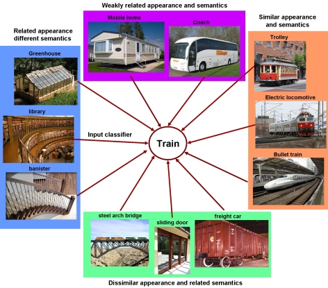
We approach feature selection from the task of discriminant linear classification (?) with novel constraints on the solution and the features. We put an upper bound on the solution weights and require it to be an affine combination of soft-categorical features, which should have on average stronger outputs on the positive class vs. the negative. We term these signed features. We present both a supervised and an almost unsupervised approach. Our supervised method is a convex constrained minimization problem, which we extend to the case of almost unsupervised learning, with a concave minimization formulation, in which the only bits of supervised information required are the feature signs. Both formulations have important sparsity and optimality properties as well as strong generalization capabilities in practice. The proposed schemes also serve as feature selection mechanisms, such that the majority of features with zero weights can be safely ignored while the remaining ones form a powerful classifier ensemble. Consider Fig. 1: here we use image-level CNN classifiers (?), pre-trained on ImageNet, to recognize trains in video frames from the YouTube-Objects dataset (?). Our method rapidly finds relevant features in a large pool.

Our main contributions are: 1) An efficient method for joint linear classifier learning and feature selection. We show that, both in theory and practice, our solutions are sparse. The number of features selected can be set to $k$ and the non-zero weights are equal to $1/k$. The simple solution enables good generalization and learning in an almost unsupervised setting, with minimal supervision. This is very different from classical regularized approaches such as the Lasso. 2) Our formulation requires minimal supervision: namely only the signs of features with respect to the target class. These signs can be estimated from a small set of labeled samples, and once determined, our method can handle large quantities of unlabeled data with excellent accuracy and generalization in practice. Our method is also robust to large errors in feature sign estimation. 3) Our method demonstrates superior performance in terms of learning time and accuracy when compared to established approaches such as AdaBoost, Lasso, Elastic Net and SVM, especially in the case of limited supervision.

Problem Formulation

We address the case of binary classification, and apply the one vs. all strategy to the multi-class scenario. Consider a set of $N$ samples, with each $i$-th sample expressed as a column vector $\mathbf{f}_{i}$ of $n$ features with values in $[0,1]$; such features could themselves be outputs of classifiers. We want to find vector $\mathbf{w}$, with elements in $[0,1/k]$ and unit $l^{1}$-norm, such that $\mathbf{w}^{T}\mathbf{f}_{i}\approx\mu_{P}$ when the $i$-th sample is from the positive class and $\mathbf{w}^{T}\mathbf{f}_{i}\approx\mu_{N}$ otherwise, with $0\leq\mu_{N}<\mu_{P}\leq 1$. For a labeled training sample $i$, we fix the ground truth target $t_{i}=\mu_{P}=1$ if positive and $t_{i}=\mu_{N}=0$ otherwise. Our novel constraints on $\mathbf{w}$ limit the impact of each individual feature $f_{j}$, encouraging the selection of features that are powerful in combination, with no single one strongly dominating. This produces solutions with good generalization power. In a later section we show that $k$ is equal to the number of selected features, all with weights $=1/k$. The solution we look for is a weighted feature average with an ensemble response that is stronger on positives than on negatives. For that, we want any feature $f_{j}$ to have expected value $E_{P}(f_{j})$ over positive samples greater than its expected value $E_{N}(f_{j})$ over negatives. We estimate its sign $\mathit{sign}(f_{j})=E_{P}(f_{j})-E_{N}(f_{j})$ from labeled samples and if it is negative we simply flip the feature: $f_{j}\leftarrow 1-f_{j}$. Expected values are estimated as the empirical average feature responses the the labeled training data available.

Supervised Learning:

We begin with the supervised learning task, which we formulate as a least-squares constrained minimization problem. Given the $N\times n$ feature matrix $\mathbf{F}$ with $\mathbf{f}^{\top}_{i}$ on its $i$-th row and the ground truth vector $\mathbf{t}$, we look for $\mathbf{w^{*}}$ that minimizes $\|\mathbf{Fw}-\mathbf{t}\|^{2}=\mathbf{w^{\top}(F^{\top}F)w}-2\mathbf{(F^{\top}t)}^{\top}\mathbf{w}+\mathbf{t}^{\top}\mathbf{t}$, and obeys the required constraints. We drop the last constant term $\mathbf{t}^{\top}\mathbf{t}$ and obtain the following convex minimization problem:

$$\mathbf{w^{*}} = \operatorname*{argmin}_{w}J(\mathbf{w})$$

$$= \operatorname*{argmin}_{w}\mathbf{w^{\top}(F^{\top}F)w}-2\mathbf{(F^{\top}t)}^{\top}\mathbf{w}$$

$$s.t.\sum_{j}w_{j}=1\;,\;w_{j}\in[0,1/k].$$

The least squares formulation is related to Lasso, Elastic Net and other regularized approaches, with the distinction that in our case individual elements of $\mathbf{w}$ are restricted to $[0,1/k]$. This leads to important properties regarding sparsity and directly impacts generalization power, as presented later.

Labeling the features not the samples:

Consider a pool of signed features correctly flipped according to their signs, which could be known a priori, or estimated from a small set of labeled data. We make the simplifying assumption that the signed features’ expected values (that is, the means of the feature responses distributions), for positive and negative samples, respectively, are close to the ground truth target values $(\mu_{P},\mu_{N})$. Note that having expected values close to the ground truth does not say anything about the distribution variance, as individual responses could sometimes be wrong. For a given sample $i$, and any $\mathbf{w}$ obeying the constraints, the expected value of the weighted average $\mathbf{w}^{\top}\mathbf{f}_{i}$ is also close to the ground truth target $t_{i}$: $E(\mathbf{w}^{\top}\mathbf{f}_{i})=\sum_{j}w_{j}E(\mathbf{f}_{i}(j))\approx(\sum_{j}w_{j})t_{i}=t_{i}$. Then, for all samples we have the expectation $E(\mathbf{F}\mathbf{w})\approx\mathbf{t}$, such that any feasible solution will produce, on average, approximately correct answers. Thus, we can regard the supervised learning scheme as attempting to reduce the variance of the feature ensemble output, as their expected value is close to the ground truth target. If we approximate $E(\mathbf{F}\mathbf{w})\approx\mathbf{t}$ into the objective $J(\mathbf{w})$, we get a new ground-truth-free objective $J_{u}(\mathbf{w})$ with the following learning scheme, which is unsupervised once the feature signs have been estimated. Here $\mathbf{M=F^{\top}F}$:

$$\mathbf{w^{*}} = \operatorname*{argmin}_{w}J_{u}(\mathbf{w})$$

$$= \operatorname*{argmin}_{w}\mathbf{w^{\top}(F^{\top}F)w}-2\mathbf{(F^{\top}(\mathbf{F}\mathbf{w}))}^{\top}\mathbf{w}$$

$$= \operatorname*{argmin}_{w}(-\mathbf{w^{\top}(F^{\top}Fw}))=\operatorname*{argmax}_{w}\mathbf{w^{\top}Mw}$$

$$\text{s.t.}\sum_{j}w_{j}=1\;,\;w_{j}\in[0,1/k].$$

Interestingly, while the supervised case is a convex minimization problem, the semi-supervised learning scheme is a concave minimization problem, which is NP-hard. This is due to the change in sign of the matrix $\mathbf{M}$. Since $\mathbf{M}$ in the almost unsupervised case could be created from larger quantities of unlabeled data, $J_{u}(\mathbf{w})$ could in fact be less noisy than $J(\mathbf{w})$ and produce significantly better local optimal solutions — a fact confirmed by experiments. Note the difference between our formulation and other, much more costly semi-supervised or transductive learning approaches based on label propagation with quadratic criterion (?) (where the quadratic term is very large, being computed from pairs of data samples, not features) or on transductive support vector machines (?). There are also methods for unsupervised feature selection, such as the regularization scheme of (?), but they do not simultaneously learn a discriminative classifier, as it is the case here.

Intuition:

Let us consider two terms involved in our objectives, the quadratic term: $\mathbf{w^{\top}Mw}=\mathbf{w^{\top}(F^{\top}F)w}$ and the linear term: $\mathbf{(F^{\top}t)}^{\top}\mathbf{w}$. Assuming that feature outputs have similar expected values, then minimizing the linear term in the supervised case will give more weight to features that are strongly correlated with the ground truth and are good for classification, even independently. Things become more interesting when looking at the role played by the quadratic term in the two cases of learning. The positive definite matrix $\mathbf{F^{\top}F}$ contains the dot-products between pairs of feature responses over the samples. In the supervised case, minimizing $\mathbf{w^{\top}(F^{\top}F)w}$ should find groups of features that are as uncorrelated as possible. Thus, they should be individually relevant due to the linear term, but not redundant with respect to each other due to the quadratic term. They should be conditionally independent given the class, an observation that is consistent with earlier research (e.g., (?; ?)). In the almost unsupervised case, the task seems reversed: maximize the same quadratic term $\mathbf{w^{\top}Mw}$, with no linear term involved. We could interpret this as transforming the learning problem into a special case of clustering with pairwise constraints, related to methods such as spectral clustering with $l^{2}$-norm constraints (?) and robust hypergraph clustering with $l^{1}$-norm constraints (?; ?). The problem is addressed by finding the group of features with strongest intra-cluster score — the largest amount of covariance. In the absence of ground truth labels, if we assume that features in the pool are, in general, correctly signed and not redundant, then the maximum covariance is attained by those whose collective average varies the most as the hidden class labels also vary.

Algorithm

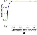
We first need to estimate the sign for each feature, using its average response over positives and negatives, respectively. Then we can set up the optimization problems to find $\mathbf{w}$. In Algorithm 1, we present the almost unsupervised method, with the supervised variant being constructed by modifying the objective appropriately. There are many possible fast methods for approximate optimization. Here we adapted the integer projected fixed point (IPFP) approach (?; ?), which is efficient in practice (Fig. 2c) and is applicable to both supervised and semi-supervised cases. The method converges to a stationary point — the global optimum in the supervised case. At each iteration IPFP approximates the original objective with a linear, first-order Taylor approximation that can be optimized immediately in the feasible domain. That step is followed by a line search with rapid closed-form solution, and the process is repeated until convergence. In practice, $10$–$20$ iterations bring us close to the stationary point; nonetheless, for thoroughness, we use $100$ iterations in all tests. See, for example, comparisons to Matlab’s quadprog run-time for the convex supervised learning case in Fig. 2 and to other learning methods in Fig. 5. Note that once the linear and quadratic terms are set up, the learning problems are independent of the number of samples and only dependent on the number $n$ of features considered, since $\mathbf{M}$ is $n\times n$ and $\mathbf{F^{\top}t}$ is $n\times 1$.

Figure 2: Optimization and sensitivity analysis: a) Sensitivity to $k$. Performance improves as features are added, is stable around the peak $k=60$ and falls for $k>100$ as useful features are exhausted. b) Features ordered by weight for $k=50$ confirming that our method selects equal weights up to the chosen $k$. c) Our method almost converges in $10$–$20$ iterations. d) Runtime of interior point method divided by ours, both in Matlab and with $100$ max iterations. All results are averages over $100$ random runs.

Algorithm 1 Learning with minimal supervision.

  Learn feature signs from a small set of labeled samples.

  Create $\mathbf{F}$ with flipped features from unlabeled data.

  Set $\mathbf{M}\leftarrow\mathbf{F^{\top}F}$.

  Find $\mathbf{w^{*}}=\operatorname*{argmax}_{w}\mathbf{w^{\top}Mw}$        s.t. $\sum_{j}w_{j}=1\;,\;w_{j}\in[0,1/k]$.

  return  $\mathbf{w^{*}}$

Theoretical Analysis:

First we show that the solutions are sparse with equal non-zero weights (P1), also observed in practice (Fig. 2b). This property makes our classifier learning also an excellent feature selection mechanism. Next, we show that simple equal weight solutions are likely to minimize the output variance over samples of a given class (P2) and minimize the error rate. This explains the good generalization power. Then we show how the error rate is expected to go towards zero when the number of considered non-redundant features increases (P3), which explains why a large diverse pool of features is beneficial. Let $J(\mathbf{w})$ be the objective for either the supervised or semi-supervised case:

Figure 3: Sensitivity analysis for Lasso: Left: sensitivity to number of features with non-zero weights in the solution. Note the higher sensitivity when compared to ours. Lasso’s best performance is achieved for fewer features, but the accuracy is worse than in our case. Right: sensitivity to lambda $\lambda$, which controls the L1-regularization penalty.

Proposition 1: Let $\mathbf{d(w)}$ be the gradient of $J(\mathbf{w})$. The partial derivatives $d(\mathbf{w})_{i}$ corresponding to those elements $w^{*}_{i}$ of the stationary points with non-sparse, real values in $(0,1/k)$ must be equal to each other.

Proof: The stationary points for the Lagrangian satisfy the Karush-Kuhn-Tucker (KKT) necessary optimality conditions. The Lagrangian is $L(\mathbf{w},\lambda,\mu,\beta)=J(\mathbf{w})-\lambda(\sum w_{i}-1)+\sum\mu_{i}w_{i}+\sum\beta_{i}(1/k-w_{i})$. From the KKT conditions at a point $\mathbf{w^{*}}$ we have:

$$\begin{array}[]{l}\mathbf{d(w^{*})}-\lambda+\mu_{i}-\beta_{i}=0,\\ \sum_{i=1}^{n}\mu_{i}w^{*}_{i}=0,\\ \sum_{i=1}^{n}\beta_{i}(1/k-w^{*}_{i})=0.\\ \end{array}$$

Here $\mathbf{w^{*}}$ and the Lagrange multipliers have non-negative elements, so if $w_{i}>0\Rightarrow\mu_{i}=0$ and $w_{i}<1/k\Rightarrow\beta_{i}=0$. Then there must exist a constant $\lambda$ such that:

$$d(\mathbf{w^{*}})_{i}=\left\{\begin{array}[]{ll}\leq\lambda,&w^{*}_{i}=0,\\ =\lambda,&w^{*}_{i}\in(0,1/k),\\ \geq\lambda,&w^{*}_{i}=1/k.\\ \end{array}\right.$$

This implies that all $w^{*}_{i}$ that are different from $0$ or $1/k$ correspond to partial derivatives $d(\mathbf{w})_{i}$ that are equal to some constant $\lambda$, therefore those $d(\mathbf{w})_{i}$ must be equal to each other, which concludes our proof.

From Proposition $1$ it follows that in the general case, when the partial derivatives of the objective error function at the Lagrangian stationary point are unique, the elements of the solution $\mathbf{w^{*}}$ are either $0$ or $1/k$. Since $\sum_{j}w^{*}_{j}=1$ it follows that the number of nonzero weights is exactly $k$, in the general case. Thus, our solution is not just a simple linear separator (hyperplane), but also a sparse representation and a feature selection procedure that effectively averages the selected $k$ (or close to $k$) features. The method is robust to the choice of $k$ (Fig. 2.a) and seems to be less sensitive to the number of features selected than the Lasso (see Fig. 3). In terms of memory cost, compared to the solution with real weights for all features, whose storage requires $32n$ bits in floating point representation, our averaging of $k$ selected features needs only $k\log_{2}n$ bits — select $k$ features out of $n$ possible and automatically set their weights to $1/k$. Next, for a better statistical interpretation we assume the somewhat idealized case when all features have equal means $(\mu_{P},\mu_{N})$ and equal standard deviations $(\sigma_{P},\sigma_{N})$ over positive (P) and negative (N) training sets, respectively.

Proposition 2: If we assume that the input soft classifiers are independent and better than random chance, the error rate converges towards $0$ as their number $n$ goes to infinity.

Proof: Given a classification threshold $\theta$ for $\mathbf{w}^{T}\mathbf{f}_{i}$, such that $\mu_{N}<\theta<\mu_{P}$, then, as $n$ goes to infinity, the probability that a negative sample will have an average response greater than $\theta$ (a false positive) goes to $0$. This follows from Chebyshev’s inequality. By a similar argument, the chance of a false negative also goes to $0$ as $n$ goes to infinity.

Proposition 3: The weighted average $\mathbf{w}^{T}\mathbf{f}_{i}$ with smallest variance over positives (and negatives) has equal weights.

Proof: We consider the case when $\mathbf{f}_{i}$’s are from positive samples, the same being true for the negatives. Then $\text{Var}(\sum_{j}w_{j}\mathbf{f}_{i}(j)/\sum_{j}w_{j})=\sum w_{j}^{2}/(\sum w_{j})^{2}\sigma^{2}_{P}$. We minimize $\sum w_{j}^{2}/(\sum w_{j})^{2}$ by setting its partial derivatives to zero and get $w_{q}(\sum w_{j})=\sum w_{j}^{2},\forall q$. Then $w_{q}=w_{j},\forall q,j$.

Figure 4: We encourage feature diversity by taking classifiers trained on 3 datasets and by looking at different parts of the input space (Type I) or different locations within the image (Types II and III).

Experimental Analysis

We evaluate our method’s ability to generalize and learn quickly from limited data, in both the supervised and the unsupervised cases. We also explore the possibility of transferring and combining knowledge from different datasets, containing video or low and medium-resolution images of many potentially unrelated classes, by working with three different types of features, as explained shortly. We focus on video classification and compare to established methods for selection and classification and report accuracies per frame. We test on the large-scale YouTube-Objects video dataset (?), with difficult sequences from ten categories (aeroplane, bird, boat, car, cat, cow, dog, horse, motorbike, train) taken in the wild. The training set contains about $4200$ video shots, for a total of $436970$ frames, and the test set has $1284$ video shots for a total of over $134119$ frames. The videos have significant clutter, with objects coming in and out of foreground focus, undergoing occlusions, extensive changes in scale and viewpoint. This set is difficult because the intra-class variation is large and sudden between video shots. Given the very large number of frames and variety of shots, their complex appearance and variation in length, presence of background clutter with many distracting objects, changes in scale, viewpoint and drastic intra-class variation, the task of learning the main category from only a few frames presents a significant challenge. We used the same training/testing split as prescribed in (?). In all our tests, we present results averaged over $30$ randomized trials, for each method. We generate a large pool of over $6000$ different features (see Fig. 4), computed and learned from three different datasets: CIFAR10 (?), ImageNet (?) and a hold-out part of the YouTube-Objects training set:

CIFAR10 features (Type I):

This dataset contains $60000$ 32$\times$32 color images in $10$ classes (airplane, automobile, bird, cat, deer, dog, frog, horse, ship, truck), with $6000$ images per class. There are $50000$ training and $10000$ test images. We randomly chose $2500$ images per class to create features. They are HOG+SVM classifiers trained on data obtained by clustering images from each class into $5$ groups using k-means applied to their HOG descriptors. Each classifier was trained to separate its own cluster from the others. We hoped to obtain, for each class, diverse and relatively independent classifiers that respond to different, naturally clustered, parts of the input space. Note that CIFAR10 classes coincide only partially ($7$ out of $10$) with the YouTube-Objects classes. Each of the $5\times 10=50$ such classifiers becomes a different feature.

YouTube-parts features (Type II):

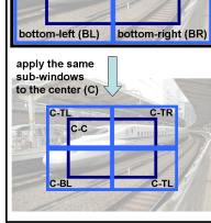
We formed a separate dataset with $25000$ images from video, randomly selected from a subset of YouTube-Objects training videos, not used in subsequent recognition experiments. Features are outputs of linear SVM classifiers using HOG applied to the different parts of each image. Each classifier is trained and applied to its own dedicated sub-window as shown in Fig. 4.

We also applied PCA to the resulted HOG, and obtained descriptors of $46$ dimensions, before passing them to SVM. For each of the $10$ classes, we have $11$ classifiers, one for each sub-window, and get a total of $110$ type II features.

ImageNet features (Type III):

We considered the soft feature outputs (before soft max) of the pre-trained ImageNet CNN features using Caffe (?), each of them over six different sub-windows: whole, center, top-left, top-right, bottom-left, bottom-right, as presented in Fig. 4. There are $1000$ such outputs, one for each ImageNet category, for each sub-window, for a total of $6000$ features. In some of our experiments, when specified, we used only $2000$ ImageNet features, restricted to the whole and center windows.

Results

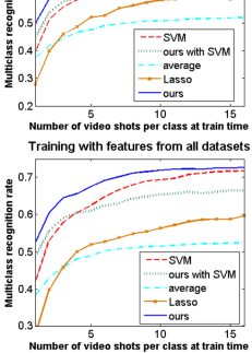
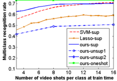
We evaluated eight methods: ours, SVM on all input features, Lasso, Elastic Net (L1+L2 regularization) (?), AdaBoost on all input features, ours with SVM (applying SVM only to features selected by our method, idea related to (?; ?; ?)), forward-backward selection (FoBa) (?) and simple averaging of all signed features, with values in $[0,1]$ and flipped as discussed before. While most methods work directly with the signed features provided, AdaBoost further transforms each feature into a weak binary classifier by choosing the threshold that minimizes the expected exponential loss at each iteration (this explains why AdaBoost is much slower). For SVM we used the LIBSVM (?) implementation version $3.17$, with kernel and parameter $C$ validated separately for each type of experiment. For the Lasso we used the latest Matlab library and validated the L1-regularization parameter $\lambda$ for each experiment. For the Elastic Net we also validated parameter alpha that combines the L1 and L2 regularizers. The results (Fig. 5) show that our method has a constant optimization time (after creating $\mathbf{F}$, and then computing $\mathbf{F^{\top}F}$). It is significantly faster than SVM, AdaBoost (time too large to show in the plot), FoBa and even the latest Matlab’s Lasso. Elastic Net, not shown in the plots to avoid clutter, was consistently slower than Lasso by at least $35\%$ and, at best, $2\%$ superior in performance to Lasso for certain parameters $alpha$. As seen, we outperform most other methods, especially in the case of limited labeled training data, when our selected feature averages generalize well and are even stronger than in combination with SVM. In the case of the almost unsupervised learning, we outperformed all other methods by a very large margin, up to over $20\%$ (Fig. 6 and Table 1). Of particular note is when only a single labeled image per class was used to estimate the feature signs, with all the other data being unlabeled (Fig. 6).

Figure 5: Accuracy and training time (in sec.) on YouTube-Objects, with varying training video shots ($10$ frames per shot and results averaged over $30$ runs). Input feature pool, row 1: $50$ type I features on CIFAR10; row 2: $110$ type II features on YouTube-Parts + $50$ CIFAR10; row 3: $2000$ type III features in ImageNet; row 4: $2160$ all features. Ours outperforms SVM, Lasso, AdaBoost and FoBa.

Table 1: Improvement in recognition of unsupervised vs. the supervised method. Experiments with adding unlabeled training data to (1,3,8,16) labeled shots (used for estimating feature signs) reveals significant improvement over the supervised learning scheme, across all trials. The first column presents the one-shot learning case, when the almost unsupervised method uses a single labeled image per class to estimate the feature signs. Results are averages (in percent) over $30$ random runs.

Training # shots	1	3	8	16
Feature I	+15.1	+16.9	+13.9	+14.0
Feature I+II	+16.7	+10.2	+6.2	+6.1
Feature III	+23.6	+11.2	+4.9	+3.3
Feature I+II+III	+24.4	+13.4	+6.7	+5.4

Figure 6: Comparison of our almost unsupervised approach to the supervised case for different methods. In our case, unsup1 uses training data in $J_{u}(\mathbf{w})$ only from the shots used by all supervised methods; unsup2 also includes frames from testing shots, with unknown test labels; oneshot is unsup2 with a single labeled image per class used only for feature sign estimation. This truly demonstrates the ability of our approach to efficiently learn with minimal supervision.

Estimating feature signs from limited data:

The performance of our almost unsupervised learning approach with signed features depends on the ability to estimate the signs of features. We evaluate the accuracy of the estimated signs with respect to the available labeled data (Fig. 7). Our experiments show that feature signs are often wrongly estimated and thus confirm that our method is robust to such errors, with a relatively stable accuracy as the quantity of labeled samples varies (Fig. 6). Note that we have compared the estimated feature signs with the ones estimated from the entire unlabeled test set of the database and present estimation accuracies, where the signs estimated from the test set were considered the empirical ground truth. The relatively large sign estimation errors reflect the large relative difference in quantity between the total amount of test data available and the small number of samples used for sign estimation. It also indicates our methods ability to learn effective feature groups in the presence of many others that have been wrongly signed.

Figure 7: For a feature sign estimation accuracy (agreement with sign estimation from the test set) of roughly $70\%$ our method manages to significantly outperform the supervised case, demonstrating its robustness and solid practical value. The first value corresponds to 1-shot-1-frame case.

Figure 8: Youtube-Objects classes similarity based on their estimated signs of features. For each pair of features we present the percent of signs of features that coincide. Note that classes that are more similar in meaning, shape or context have, on average more signs that coincide. These signs were estimated from all training data.

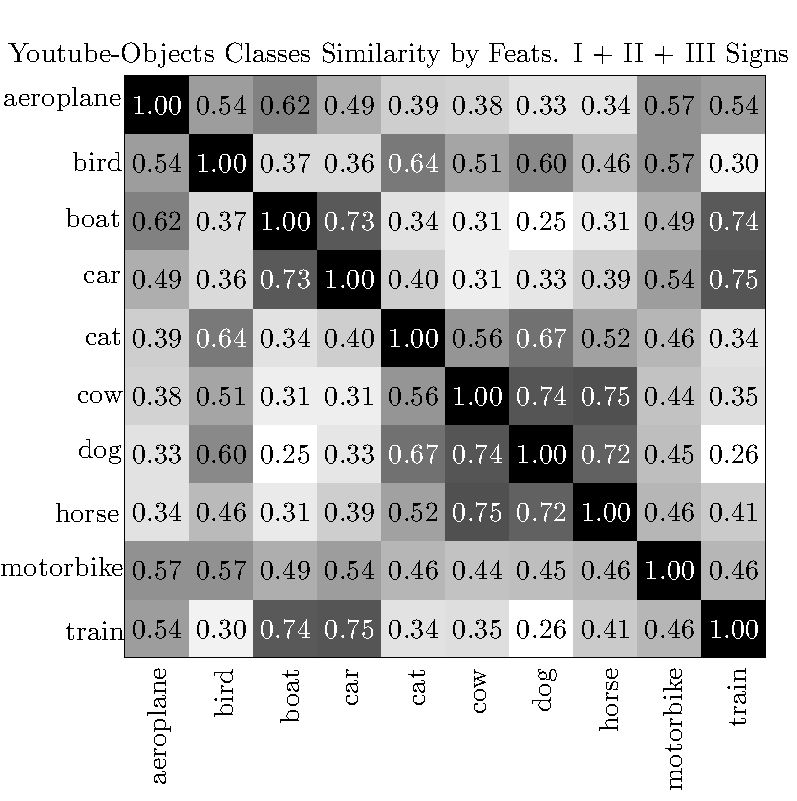
An interesting direction for future work is to explore the possibility of borrowing feature signs from classes that are related in meaning, shape or context. We have performed some experiments and compared the estimated feature signs between classes (see Figure 8). Does the plane share more feature signs with the bird, or with another man-made class, such as the train? The possibility of sharing or borrowing feature signs from other classes could pave the way for a more unsupervised type of learning, where we would not need to estimate the signs from labeled data of the specific class. The results in Figure 8 indicate that, indeed, classes that are closer in meaning share more signs than classes that mean very different things. For example, the class aeroplane shares most signs with boat, motorbike, bird, train, bird with cat, dog, motorbike, aeroplane, cow, boat with train, car aeroplane, and car with train, boat, motorbike. We also have cat: dog, bird, cow, horse, cow: horse, dog, cat, bird, dog: cow, horse, cat, bird, horse: cow, dog, cat, motorbike: aeroplane, bird, car, and train: car, boat, aeroplane, for the remaining classes. We notice that indeed classes that are similar in meaning, appearance or context, such as animals, or man-made categories, share more signs among themselves than classes that are very different. These experiments indicate the deeper conceptual difference between labeling features and not samples. As our method can be effective even in case of sign estimation errors, it could relay on some sort of smart sign guessing and then learn from completely unsupervised data - this would reduce the amount of supervision to a minimum, and get closer to the natural limits of learning in strongly unsupervised environments.

Intuition regarding the selected features:

Figure 9: Visualization of classifiers selected by our method for each target concept (not samples of images retrieved for a given concept). Each row corresponds to a class from the YouTube-Objects dataset and the images in a given row show an image from the most frequently selected ImageNet classifiers (input features) that contribute to that class—specifically the classes that were always selected over 30 independent experiments ($k=50$, 10 frames per shot and 10 random shots for training). The far right graph in each row shows the probability of selecting these 50 features for the given class. Note the stability of the selection process. Also note the connection between the selected ImageNet classifier and the target YouTube object class in terms of appearance, context or geometric part-whole relationships. We find two aspects particularly interesting: 1) the consistent selection of the same classes, even for small random training sets and 2) the fact that semantically unrelated classes contribute to classification, based on their shape and appearance similarity.

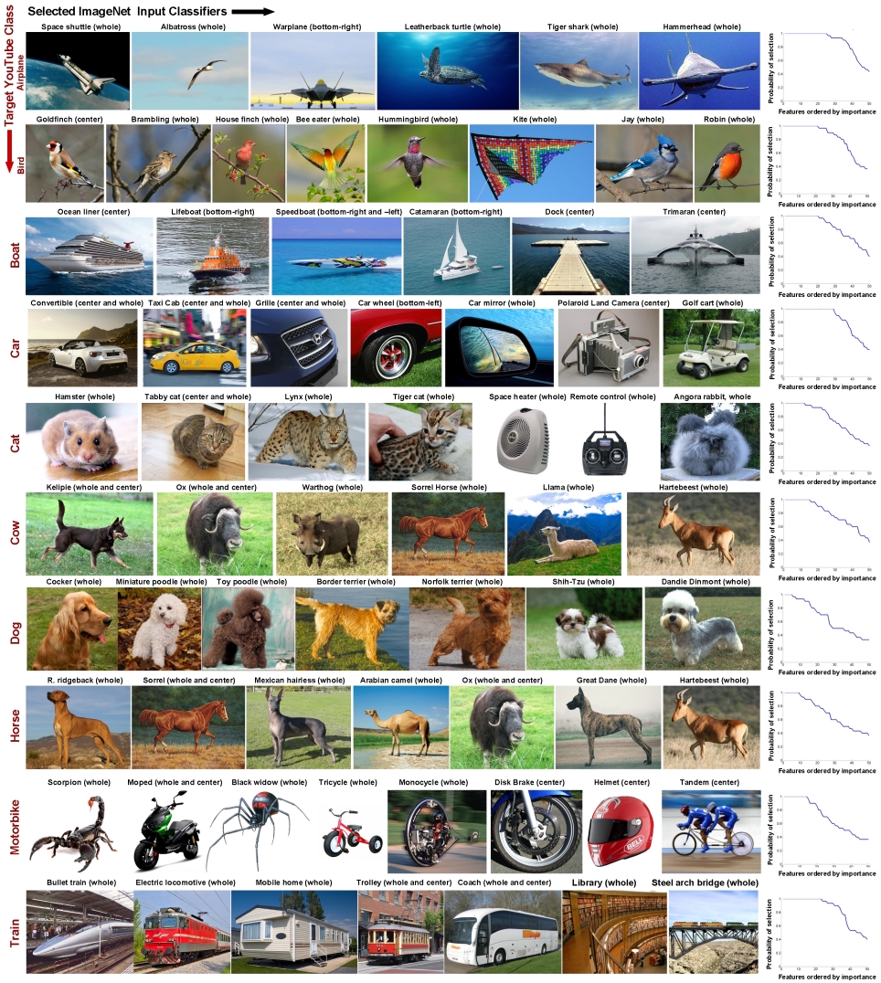
Another interesting finding (see Fig. 9) is the consistent selection of diverse input Type III features that are related to the target class in surprising ways: 1) similar w.r.t. global visual appearance, but not semantic meaning — banister :: train, tiger shark :: plane, Polaroid camera :: car, scorpion :: motorbike, remote control :: cat’s face, space heater :: cat’s head; 2) related in co-occurrence and context, but not in global appearance — helmet vs. motorbike; 3) connected through part-to-whole relationships — {grille, mirror and wheel} :: car; or combinations of the above — dock :: boat, steel bridge :: train, albatross :: plane. The relationships between the target class and the selected features could also hide combinations of many other factors. Meaningful relationships could ultimately join together correlations along many dimensions, from appearance to geometric, temporal and interaction-like relations. Since categories share shapes, parts and designs, it is perhaps unsurprising that classifiers trained on semantically distant classes that are visually similar can help improve learning and generalization from limited data. Another interesting aspect is that the classes found are not necessarily central to the main category, but often peripheral, acting as guardians that separate the main class from the rest. This is where feature diversity plays an important role, ensuring both separation from nearby classes as well as robustness to missing values. This aspect is also related to the idea of borrowing features from related, previously learned classes. Thus, in cases where there is insufficient supervised data for a particular new class, sparse averages of reliable, old classifiers and features can be an excellent way to combine previous knowledge. Consider the class cow in Fig. 9. Although “cow” is not present in the $1000$ label set, our method is able to learn the concept by combining existing classifiers.

Comparison with Linear SVM:

Figure 10: Supervised learning: Our method generalizes better (training and test errors are closer) compared to SVM or in combination with SVM on limited training data.

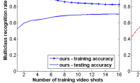
In our experiments, the supervised learning method generalized significantly better, on average, than SVM or in combination with SVM in cases of very limited labeled training data. We believe that this is due to the power of feature averages, as also indicated by our theoretical results presented earlier. Our formulation is expected to discover features that are independent and strong as a group, not necessarily individually. That is why we prefer to give all selected features equal weight than to put too much faith into a single strong feature, especially in the case of limited training data. As seen in Figure 10, our supervised approach generalizes better than SVM or in combination with SVM, as reflected by the performance differences between the testing and training cases. Note that we have used a very recent SVM library (libsvm-3.17) with kernel and parameter $C$ validated separately for each type of experiment - in our experiments the linear kernel performed the best. We can also see that our method often generalizes from just $1$ frame per video shot, for a total of $8$ positive training frames per class in the experiments in Fig. 11.

Figure 11: Supervised learning: avg. test recognition accuracy over $30$ independent experiments of our method as we vary the number of training frames uniformly sampled from $8$ random training video shots. Note how well our method generalizes from just $1$ frame per video shot, for a total of $8$ positive training frames per class.

Varying the amount of unsupervised data:

We evaluated the influence of varying amounts of unlabeled data used for the (almost) unsupervised learning method. We present the following experimental setup: first, we randomly split the unlabeled test data into two equal sets of frames, $S_{A}$ and $S_{B}$. We have used one set of unlabeled frames $S_{A}$ for unsupervised learning and the other set $S_{B}$ for testing. While keeping the test frames set $S_{B}$ constant, and $8$ labeled video shots per class for feature sign estimation from the training set (with $10$ evenly spaced frames per shot), we varied the amount of unlabeled data used for unsupervised learning, by varying the percentage of unlabeled frames used from $S_{A}$. We present results over $30$ random runs in Figure 12 and Table 2.

Table 2: Testing accuracy when varying the quantity of unlabeled data used for unsupervised learning. We used $8$ video shots per class with 10 frames each, for estimating the signs of the features. Results are averages over $30$ random runs.

.

Unsupervised data	Features I	Features I+II	Features III	Features I+II+III
Train + 0% test $S_{A}$	30.86%	48.96%	49.03%	53.71%
Train + 25% test $S_{A}$	41.26%	55.50%	66.90%	72.01%
Train + 50% test $S_{A}$	42.72%	56.66%	71.31%	76.78%
Train + 75% test $S_{A}$	42.88%	57.24%	73.65%	77.39%
Train + 100% test $S_{A}$	43.00%	57.44%	74.30%	78.05%

Figure 12: Testing accuracy vs amount of unlabeled data used for unsupervised learning. Note that the performance almost reaches a plateau after a relatively small fraction of unlabeled frames are added.

Discussion and Conclusions

We present a fast feature selection and learning method with minimal supervision, and we apply it to video classification. It has strong theoretical properties and excellent generalization and accuracy in practice. The crux of our approach is its ability to learn from large quantities of unlabeled data once the feature signs are determined, while being very robust to feature sign estimation errors. A key difference between our features signs and the weak features used by boosting approaches such as AdaBoost, is that in our case the sign estimation requires minimal labeling and that the sign is the only bit of supervision needed. Adaboost requires large amounts of training data to carefully select and weigh new features. This aspect reveals a key insight: being able to approximately label the features and not the data, is sufficient for learning. With a formulation that permits very fast optimization and effective learning from large heterogeneous feature pools, our approach provides a useful tool for many other recognition tasks, and it is suited for real-time, dynamic environments. Thus it could open doors for new and exciting research in machine learning, with both practical and theoretical impact.
Acknowledgements: This work was supported in part by CNCS-UEFICSDI, under project PNII PCE-2012-4-0581.

References

- [Bengio, Delalleau, and Roux 2006] Bengio, Y.; Delalleau, O.; and Roux, N. L. 2006. Label propagation and quadratic criterion. Semi-sup. learning.
- [Breiman 1996] Breiman, L. 1996. Bagging predictors. Machine learning 24(2).
- [Bulo and Pellilo 2009] Bulo, S., and Pellilo, M. 2009. A game-theoretic approach to hypergraph clustering. In NIPS.
- [Chang and Lin 2011] Chang, C.-C., and Lin, C.-J. 2011. LIBSVM: a library for support vector machines. ACM TIST 2(27).
- [Criminisi, Shotton, and Konukoglu 2012] Criminisi, A.; Shotton, J.; and Konukoglu, E. 2012. Decision forests: A unified framework for classification, regression, density estimation, manifold learning and semi-supervised learning. CGV 7(2–3).
- [Deng et al. 2009] Deng, J.; Dong, W.; Socher, R.; Li, L.; Li, K.; and Fei-Fei, L. 2009. ImageNet: A large-scale hierarchical image database. In CVPR.
- [Dietterich 2000] Dietterich, T. 2000. Ensemble methods in machine learning. Springer.
- [Duda and Hart 1973] Duda, R., and Hart, P. 1973. Pattern classification and scene analysis. Wiley.
- [Freund and Schapire 1995] Freund, Y., and Schapire, R. 1995. A decision-theoretic generalization of on-line learning and an application to boosting. In COLT.
- [Guyon and Elisseeff 2003] Guyon, I., and Elisseeff, A. 2003. An introduction to variable and feature selection. JMLR 3:1157–1182.
- [Hansen and Salamon 1990] Hansen, L., and Salamon, P. 1990. Neural network ensembles. PAMI 12(10).
- [Jia et al. 2014] Jia, Y.; Shelhamer, E.; Donahue, J.; Karayev, S.; Long, J.; Girshick, R.; Guadarrama, S.; and Darrell, T. 2014. Caffe: Convolutional architecture for fast feature embedding. In ACM Multimedia.
- [Joachims 1999] Joachims, T. 1999. Transductive inference for text classification using support vector machines. In ICML.
- [Kira and Rendell 1992] Kira, K., and Rendell, L. 1992. The feature selection problem: Traditional methods and a new algorithm. In AAAI.
- [Krizhevsky and Hinton 2009] Krizhevsky, A., and Hinton, G. 2009. Learning multiple layers of features from tiny images. TR, Univ. of Toronto.
- [Kwok and Carter 1990] Kwok, S., and Carter, C. 1990. Multiple decision trees. Uncertainty in Artificial Intelligence.
- [Leordeanu and Sminchisescu 2012] Leordeanu, M., and Sminchisescu, C. 2012. Efficient hypergraph clustering. In AISTATS.
- [Leordeanu, Hebert, and Sukthankar 2009] Leordeanu, M.; Hebert, M.; and Sukthankar, R. 2009. An integer projected fixed point method for graph matching and map inference. In NIPS.
- [Liu, Latecki, and Yan 2010] Liu, H.; Latecki, L.; and Yan, S. 2010. Robust clustering as ensembles of affinity relations. In NIPS.
- [Ng 1998] Ng, A. 1998. On feature selection: learning with exponentially many irrelevant features as training examples. In ICML.
- [Nguyen and De la Torre 2010] Nguyen, M., and De la Torre, F. 2010. Optimal feature selection for support vector machines. Pattern recognition 43(3).
- [Prest et al. 2012] Prest, A.; Leistner, C.; Civera, J.; Schmid, C.; and Ferrari, V. 2012. Learning object class detectors from weakly annotated video. In CVPR.
- [Pudil, Novovičová, and Kittler 1994] Pudil, P.; Novovičová, J.; and Kittler, J. 1994. Floating search methods in feature selection. Pattern recognition letters 15(11).
- [Rolls and Deco 2010] Rolls, E., and Deco, G. 2010. The noisy brain: stochastic dynamics as a principle of brain function, volume 34. Oxford Univ. Press.
- [Sarkar and Boyer 1998] Sarkar, S., and Boyer, K. 1998. Quantitative measures of change based on feature organization: Eigenvalues and eigenvectors. CVIU 71(1):110–136.
- [Siedlecki and Sklansky 1989] Siedlecki, W., and Sklansky, J. 1989. A note on genetic algorithms for large-scale feature selection. Pattern recognition letters 10(5).
- [Tibshirani 1996] Tibshirani, R. 1996. Regression shrinkage and selection via the lasso. Journal of the Royal Statistical Society. 267–288.
- [Vasconcelos 2003] Vasconcelos, N. 2003. Feature selection by maximum marginal diversity: optimality and implications for visual recognition. In CVPR.
- [Vogel 2002] Vogel, C. R. 2002. Computational methods for inverse problems, volume 23. SIAM.
- [Weston et al. 2000] Weston, J.; Mukherjee, S.; Chapelle, O.; Pontil, M.; Poggio, T.; and Vapnik, V. 2000. Feature selection for SVMs. In NIPS, volume 12.
- [Yang et al. 2011] Yang, Y.; Shen, H. T.; Ma, Z.; Huang, Z.; and Zhou, X. 2011. L2, 1-norm regularized discriminative feature selection for unsupervised learning. In IJCAI.
- [Zhang 2009] Zhang, T. 2009. Adaptive forward-backward greedy algorithm for sparse learning with linear models. In NIPS.
- [Zhao and Yu 2006] Zhao, P., and Yu, B. 2006. On model selection consistency of lasso. JMLR 7.
- [Zou and Hastie 2005] Zou, H., and Hastie, T. 2005. Regularization and variable selection via the elastic net. Journal of the Royal Statistical Society: Series B (Statistical Methodology) 67(2).