Jet shapes for boosted jet two-prong decays from first-principles

Abstract

Several boosted jet techniques use jet shape variables to discriminate the multi-pronged signal from Quantum Chromodynamics backgrounds. In this paper, we provide a first-principles study of an important class of jet shapes all of which put a constraint on the subjet mass: the mass-drop parameter ($\mu^{2}$), the $N$-subjettiness ratio ($\tau_{21}^{(\beta=2)}$) and energy correlation functions ($C_{2}^{(\beta=2)}$ or $D_{2}^{(\beta=2)}$). We provide analytic results both for QCD background jets as well as for signal processes. We further study the situation where cuts on these variables are applied recursively with Cambridge-Aachen de-clustering of the original jet. We also explore the effect of the choice of axis for $N$-subjettiness and jet de-clustering. Our results bring substantial new insight into the nature, gain and relative performance of each of these methods, which we expect will influence their future application for boosted object searches.

1 Introduction

In recent years jet substructure studies have received unprecedented attention and have been the focus of many theoretical and experimental studies. Most of this research has been carried out in the direct context of boosted new particle searches at the LHC. For reviews and detailed studies we refer the reader to Refs. Abdesselam:2010pt ; Altheimer:2012mn ; Altheimer:2013yza ; Adams:2015hiv and references therein.

The basic ideas that underpin such studies are simple to understand. A high $p_{T}$ resonance with a mass $m\ll p_{T}$ will exhibit collimated decays where in a significant fraction of events the decay products would be reconstructed in a single “fat” jet. Tagging signal jets and removing jets arising from QCD background will thus rely crucially on detailed information about the jets themselves. In this context it is clear that valuable information will be obtained by studying the internal structure of jets in some detail.

Let us for example contrast the two-pronged hadronic decays of an electroweak boson (W/Z/H) with $1\to 2$ QCD splittings. QCD emission probabilities are infrared enhanced, favouring soft splittings, and hence a QCD jet would typically consist of a single hard prong. On the other hand decays of electroweak bosons show no preference for soft splittings and this results in a more symmetric energy sharing which gives rise to jets with a characteristic two-pronged internal structure. Another important difference results from the colour neutral nature of electroweak bosons which results in a strong suppression of radiation at angles that are large compared to the opening angle between the hard decay products. Soft large-angle radiation in a signal jet would thus typically arise from emissions that are uncorrelated with the decay of the electroweak boson in question i.e. from initial state radiation (ISR) and underlying event (UE) as well as from pile-up. Such radiation serves to degrade signal peaks making them less visible and also pushes up the masses of background jets. It is therefore also desirable to eliminate this radiation. In the above context the two principal aims of a substructure analysis therefore emerge as identification of two hard prongs (tagging) and removal of uncorrelated soft radiation (grooming).

In recent years there have been many tools developed to achieve the above aims of tagging and grooming jets. These include the mass-drop+filtering methods Butterworth:2008iy , trimming Thalertrim and pruning Ellis:2009su ; Ellis:2009me amongst a whole host of other techniques. Monte Carlo event generator studies involving several of these techniques can be found in Refs. Abdesselam:2010pt ; Altheimer:2012mn ; Altheimer:2013yza ; Adams:2015hiv and the original references.

Somewhat more recently there has also been the emergence of jet shape variables that directly attempt to quantify the $N$-pronged nature of a fat jet. Examples include the $N$-subjettiness variables Thaler:2010tr ; Kim:2010uj ; Thaler:2011gf and the $N$-point energy correlation functions (ECFs) Larkoski:2013eya ; Larkoski:2014gra , both of which are designed to take on small values for particle configurations corresponding to $N$ collimated subjets of a fat jet, which one can naturally associate to an $N$-pronged decay. These techniques typically put constraints on the gluon radiation patterns in a jet. We expect this to have a good discriminating power both at small and large angles because gluon radiation is different for colour-neutral bosons compared to coloured QCD jets. At small angles, gluon radiation tends to be larger in QCD jets, made of a mixture of quarks and gluons, than in resonances, which decay mostly into quarks. At large angles, this is an even bigger effect since one expects a strong suppression of the radiation from collimated colour-neutral resonance decays compared to QCD jets. It is interesting to notice at this stage that the large-angle region, which shape variables try to constrain, is also the region that is sensitive to initial-state radiation and the underlying event. One typically uses grooming techniques to mitigate these effects and, therefore, one may wonder about the effectiveness of shape variable constraints when combined with grooming.

For studies involving two-pronged (W/Z/H) signal jets the $N$-subjettiness ratio $\tau_{21}^{(\beta)}=\tau_{2}^{(\beta)}/\tau_{1}^{(\beta)}$ and the ECF $C_{2}^{(\beta)}$ are known to provide good discrimination between signal and background, where $\beta$ is a parameter (angular exponent) that enters the definition of both variables. We shall provide precise definitions of these variables in the following section.

There have also been several detailed studies carried out for both $\tau_{21}$ and $C_{2}$ in the literature. Again, nearly all of these studies have been done using Monte Carlo event generator tools. As examples we refer the reader to the work carried out in the original references Thaler:2010tr ; Thaler:2011gf while for more recent studies also including the implementation of these variables in multivariate combinations we refer to Ref. Adams:2015hiv .

In contrast our principal aim here is to carry out analytical calculations for the above variables, based on the first principles of QCD. Such calculations have, for instance, been carried out for the mass-drop, pruning and trimming methods Dasgupta:2013ihk and provided considerable new insight into the performance of those tools over and above what could be gained purely from Monte Carlo methods. We would therefore expect a similar level of information from analytical studies of the shape variables considered here. For our calculations in this paper we shall make the choice of $\beta=2$, i.e. focus on $\tau_{21}^{(\beta=2)}$ and $C_{2}^{(\beta=2)}$ for which calculations are relatively straightforward to perform. Detailed numerical studies of the dependence on $\beta$ have been carried out in particular for $C_{2}^{(\beta)}$, in Ref. Larkoski:2013eya . These studies found that in the transverse momentum range $p_{T}\in\left[400,500\right]$ GeV for jet masses relevant to W/Z/H tagging, optimal $\beta$ values ranged between 1.5 and 2. For larger masses the optimal $\beta$ values were found to be smaller. An analytical understanding of the $\beta$ dependence of discrimination power would also be desirable but is left to future work.

As we shall show explicitly later in the article, cuts on $\tau_{21}^{(\beta=2)}$ and $C_{2}^{(\beta=2)}$ effectively serve to constrain subjet masses. Another similar variable, that has been far less investigated in the literature, is the parameter $\mu^{2}$ of the mass-drop tagger (MDT) Butterworth:2008iy . This is obtained by declustering a jet into two subjets and taking the ratio of the squared jet mass for the heavier subjet to that for the original jet. The original mass drop tagger uses a cut on $\mu^{2}$ along with an energy cut designed to discriminate against soft splittings i.e. the $y_{cut}$ parameter of the MDT. It was shown in Ref. Dasgupta:2013ihk that in fact in the presence of the $y_{cut}$ condition the dependence on $\mu^{2}$ could essentially be neglected. In the present article we instead study the dependence on $\mu^{2}$ without any $y_{cut}$ requirement and compare the discriminating power it provides, to that from similar variables i.e. $\tau_{21}^{(\beta=2)}$ and $C_{2}^{(\beta=2)}$. Note that while the standard mass-drop tagger recurses, successively undoing the last step of a Cambridge/Aachen clustering, until the cut on $\mu^{2}$ (and the $y_{cut}$ condition) is satisfied here we study both recursive and non-recursive variants for each of the shape variables.

We carry out analytical studies for the jet mass distributions of QCD background jets with cuts on shape variables $v<v_{\rm max}$, with $v=\tau_{21},C_{2}$ and $\mu^{2}$. We also study the probability for signal jets to pass the same cuts. We define $\rho=m^{2}/(p_{T}^{2}R^{2})$, with $m$ being the jet mass and work in the limit $\rho\ll 1$ (relevant for boosted object studies) and $v_{max}\ll 1$ which is desirable to separate two-pronged structures from QCD background. Our analytical results aim only to capture leading-logarithmic accuracy although we also retain several sources of next-to–leading logarithmic corrections. We test our analytical results by comparing to fixed-order results from EVENT2 Catani:1996vz ; event2 to results from parton shower Monte Carlos and additionally carry out pure Monte Carlo studies of the impact of non-perturbative corrections. Since non-perturbative corrections are found to be large, we further examine with Monte Carlo studies the impact of grooming with SoftDrop Larkoski:2014wba . This shows an important reduction of the non-perturbative effects. To avoid diluting the main message of this paper with additional technical considerations, we defer the study of groomed jet shapes to a forthcoming work.

Note that some level of analytic understanding for jet shapes already exists. For example, studies of the lowest-order Energy-Correlation Functions, $C_{1}^{\beta}$, have been carried out in Ref. Larkoski:2013eya . Also, in the framework of Soft-Collinear Effective Theory (SCET) Bauer:2000yr ; Bauer:2001ct ; Bauer:2001yt and its extension SCET₊ Bauer:2011uc , results for $N$-subjettiness have been obtained at the N³LL accuracy for signal jets Abbate:2010xh and studies of the Energy-Correlation Functions $C_{2}^{\beta}$ and $D_{2}^{\beta}$ Larkoski:2015kga appeared as the present paper was being finalised. In contrast, rather than providing a high-accuracy calculation of a given method, the main aim of our work is a transparent comparison of different shapes for both signal and background jets with phenomenological applications in mind.

With that in mind, it is however interesting to compare our approach and results to what is obtained for $D_{2}$ in Ref. Larkoski:2015kga . Besides using different approaches (SCET-based v. more standard pQCD language), the main difference between this work and Ref. Larkoski:2015kga is that, to the best of our understanding in terms of the variable $\rho$ and $D_{2}$, the latter provides a NLL resummation in $\rho$, regardless of the value of $D_{2}$ while our approach assumes small $D_{2}$ and treats $\log(D_{2})$ and $\log(\rho)$ on an equal footing. Therefore, the calculation in Ref. Larkoski:2015kga has likely a higher accuracy, at least in the region used in many phenomenological applications. However, it is limited to $D_{2}$ while our main goal here is to discover the source of and address the main diffferences between various shapes. The results of Ref. Larkoski:2015kga require at least four numerical integration (compared to a single one for our results), which, keeping in mind our purposes, makes a physical interpretation more involved.

This article is organised as follows: In the next section we provide detailed definitions of the shapes mentioned above. Following this, in section 3, we discuss the general form of the results obtained for all the shapes under consideration, both for signal and background jets. In section 4 we perform the detailed calculations for background jets for both non-recursive and recursive variants for each shape variable. In the same section we compare the expansion of our results to fixed-order results from EVENT2, as a check on our calculations. We also carry out comparisons to results from Pythia with only final state radiation (FSR) turned on, to give a direct comparison against our calculations. In section 5 we perform the calculations, checks and comparisons to Monte Carlo for signal jets. Following this, in section 6 we study the impact of non-perturbative corrections where we note the significant contributions from initial state radiation and the underlying event in particular. In order to obtain better control over such effects we combine shape variable studies with grooming using SoftDrop and study the impact on both signal and background efficiencies. In section 7 we discuss our findings in detail including an assessment of the comparative performance of all the shapes studied here. Finally we present our conclusions.

2 Radiation-constraining jet shapes

Among a large family of jet shapes, this paper will identify and focus on a series of variables all of which place constraints on the subjet mass. In this category, we will study the following three variables:

• $N$-subjettiness computed with $\beta=2$, $\tau_{21}^{(\beta=2)}=\tau_{2}^{(\beta=2)}/\tau_{1}^{(\beta=2)}$ with $\tau_{N}^{(\beta=2)}$ defined as Thaler:2010tr ; Stewart:2010tn

  $$\tau_{N}^{(\beta=2)}=\frac{1}{p_{t,\rm jet}R^{2}}\sum_{i\in\rm jet}p_{t,i}{\rm min}_{a_{1}\dots a_{N}}(\theta_{ia_{1}}^{2},\dots,\theta_{ia_{N}}^{2}),$$ (1)

  where the sum runs over all the constituents of a given jet and $a_{1},\dots,a_{N}$ denote the partition axes. While the choice $\beta=1$ is more common in experimental studies at the LHC — likely because of an expected smaller sensitivity to non-perturbative effects —, analytic studies have thus far mostly focused on $\beta=2$. As argued eariler, the latter is expected to give better discriminative power. We decided to choose $\beta=2$ for the present study because in that case, $\tau_{N}$ acts like a measure of the subjet mass which allows for a direct comparison with the mass-drop $\mu^{2}$ cut. w To fully define $\tau_{21}$, we still need to specify our choice for the partition axes $a_{1},\dots,a_{N}$ in (1). We shall consider the following three options:

  • the optimal axes which should minimise $\tau_{N}$;

  • the $k_{t}$ axes obtained by clustering the jet with the $k_{t}$ algorithm Catani:1991hj ; Catani:1993hr ; Ellis:1993tq and taking the $N$ exclusive subjets;

  • the generalised-$k_{t}$ axes with $p=1/2$ (gen-$k_{t}(1/2)$) obtained by clustering the jet with the generalised-$k_{t}$ algorithm (see Section 4.4 of fastjet-manual ), with its extra parameter $p$ set to $1/2$, and taking the $N$ exclusive subjets.

  The third option is new and leads to similar performance to the optimal axes at much smaller computational cost. The motivation to look into gen-$k_{t}(1/2)$ axes is that its distance measure behaves again like a mass, as does $\tau_{21}^{\beta=2}$, and we can expect the resulting axes to be very close to the optimal axes. More generally, for $\tau_{21}^{\beta}$ with a generic $\beta$, we would expect the generalised-$k_{t}$ axes with $p=1/\beta$ to give a close-to-optimal result.

• a version of the mass-drop parameter Butterworth:2008iy , $\mu^{2}$ which, given two subjets $j_{1}$, $j_{2}$ in a given jet $j$ is defined as $\mu^{2}={\rm max}(m_{j_{1}}^{2},m_{j_{2}}^{2})/m_{j}^{2}$. In its original formulation, the cut on $\mu^{2}$ was applied in a recursive de-clustering of a jet obtained with the Cambridge/Aachen (C/A) algorithm Dokshitzer:1997in ; Wobisch:1998wt . The present definition of $\mu^{2}$ is however defined non-recursively, i.e. as a cut that the jet $j$ satisfies, or not, without any further de-clustering if it does not. Similarly to the definition of the $N$-subjettiness axes, we need to specify the procedure to separate the jet $j$ into two subjets $j_{1}$, $j_{2}$. We will denote by $\mu_{p}^{2}$ the result obtained by undoing the last step of a generalised-$k_{t}$ clustering, with extra parameter $p$, of the jet $j$. We shall concentrate on $\mu_{1/2}^{2}$, since it follows the ordering in mass, and $\mu_{0}^{2}$ since it corresponds to the historical choice.

• the energy correlation function double ratio. Here we again use $\beta=2$, which will be kept fixed here, and define Larkoski:2013eya ,

  $$e_{2} =\frac{1}{p_{T}^{2}R^{2}}\sum_{i<j\in\rm jet}p_{t,i}p_{t,j}\theta_{ij}^{2},$$ (2)

  $$e_{3} =\frac{1}{p_{T}^{3}R^{6}}\sum_{i<j<k\in\rm jet}p_{t,i}p_{t,j}p_{t,k}\theta_{ij}^{2}\theta_{ik}^{2}\theta_{jk}^{2},$$ (3)

  and work with $C_{2}=e_{3}/e_{2}^{2}$. Note that, at the order of accuracy targeted in this paper, we can alternatively use the recently-proposed $D_{2}=e_{3}/e_{2}^{3}$, Larkoski:2014gra , since, up to our accuracy, they only differ by a rescaling by the total jet mass.

For any of these three shapes, $v$, a cut of the form $v<v_{\rm cut}$ is expected to show good performance in discriminating two-pronged boosted objects from standard QCD jets. Note also that, if the cut is not satisfied, the jet is discarded.

Additionally, we shall also consider the cases where one of the three shape constraints introduced above is applied recursively. By this we mean that, for a shape $v$, we apply the following procedure:

1. recluster the jet $j$ with the C/A algorithm,

2. compute $v$ from $j$; if $v<v_{\rm cut}$, $j$ is the result of the procedure and exit the loop,

3. undo the last step of the clustering to get two subjets $j_{1}$ and $j_{2}$, define the hardest of $j_{1}$ and $j_{2}$ (in terms of their $p_{t}$) as the new $j$ and go back to 2.

This is of course motivated by the original mass-drop tagger proposal Butterworth:2008iy , where a cut was placed on the $\mu^{2}$ parameter. We have to note that, here, the recursion follows the hardest branch, as suggested in the modified version of the mass-drop tagger Dasgupta:2013ihk , rather than the most massive one, as in the original proposal.

3 Generic structure of the results

For QCD jets, there are two basic physical quantities that we will be interested in: the jet mass distribution after applying a given fixed, recursive or not, cut on one of the shapes described in the previous section; or the distribution of a jet shape for a given fixed value of the jet mass. The latter situation only applies to the non-recursive cases.

For signal jets, we are interested in jets of a fixed mass so the calculation will mostly focus on what fraction of these jets satisfy the constraint on the jet shape $v$, hence on the distribution of $v$ for an object of a given mass. Jets which fail the constraint on $v$ will be discarded.

Our calculations apply to the boosted regime, where the jet transverse momentum is much larger than its mass. In that context, it is convenient to introduce $\rho=m^{2}/(p_{t}R)^{2}$, with $R$ the radius of the jet. The boosted regime means that we can take the limit $\rho\ll 1$. Furthermore, in this work, we shall focus on two-pronged decays, where we expect that the radiation-constraining shapes introduced above would be smaller for signal jets than for the QCD background. It is therefore natural to start the study of these shapes in the limit where they are small. In the following we shall thus also assume that the cut on the shape is small compared to 1. In this limit, we focus on the leading double logarithm for which soft and collinear emissions can be considered as strongly ordered and the mass of the jet is dominated by the strongest of these emissions. Throughout the paper, we will therefore assume that this emission, dominating the mass of the jet, occurs at an angle $R\theta_{1}$ and with a fraction $z_{1}$ of the jet transverse momentum $p_{t}$. This has to satisfy the constraint $z_{1}(1-z_{1})\theta_{1}^{2}=\rho$, where, for QCD jets we can neglect the $(1-z_{1})$ factor which would only lead to subleading power corrections in $\rho$.

All the shapes, $v$, that we consider put constraints on additional emissions. This means that we can always consider, as a starting point, a system made of two partons — the “leading parton $p_{0}$” initiating the jet and the “first, leading, emission $p_{1}$” which sets the jet mass for QCD jets, or the two prongs of a massive boson decay for signal jets — and study additional radiation from this system.

In the leading-logarithmic approximation, the constraint on radiation will always take the form of a Sudakov suppression coming on top of the mass requirement. For QCD jets, the mass distribution with a cut on $v$ can always be written as

$$\left.\frac{\rho}{\sigma}\frac{{\rm d}\sigma}{{\rm d}\rho}\right|_{<v} =\int_{\rho}^{1}\frac{d\theta_{1}^{2}}{\theta_{1}^{2}}\int_{\rho}^{1}dz_{1}\,P(z_{1})\,\rho\,\delta(z_{1}\theta_{1}^{2}-\rho)\frac{\alpha_{s}(z_{1}\theta_{1}p_{t}R)}{2\pi}e^{-R_{\rm mass}(\rho)-R_{v}(z_{1},\rho)}$$

$$=\int_{\rho}^{1}dz_{1}\,P(z_{1})\,\frac{\alpha_{s}(\sqrt{z_{1}\rho}\,p_{t}R)}{2\pi}e^{-R_{\rm mass}(\rho)-R_{v}(z_{1},\rho)}.$$ (4)

In the above $R_{\rm mass}(\rho)$ is the Sudakov resumming the leading $\log(1/\rho)$ contributions to the plain jet mass and $R_{v}(z_{1},\rho)$ the extra contribution coming from the additional cut on $v$.

In the approximation we shall be working at, instead of $P(z_{1})$, it is sufficient to consider its leading logarithmic contribution from its $2C_{R}/z_{1}$ term and a subleading hard collinear contribution $2C_{R}B_{i}\delta(z_{1}-1)$, where $C_{R}$ is the colour charge of a jet initiated by a parton of flavour $i$ and $B_{i}$ is the integral of the non-singular part of the splitting function:

$$B_{q} =\int_{0}^{1}dz\,\left(\frac{1}{2C_{F}}P_{qq}(z)-\frac{1}{z}\right)=-\frac{3}{4},$$ (5)

$$B_{g} =\int_{0}^{1}dz\,\left(\frac{P_{gg}(z)+2n_{f}P_{qg}(z)}{2C_{A}}-\frac{1}{z}\right)=-\frac{11C_{A}-4n_{f}T_{R}}{12C_{A}}.$$ (6)

Eq. (3) can therefore be replaced by

$$\left.\frac{\rho}{\sigma}\frac{{\rm d}\sigma}{{\rm d}\rho}\right|_{<v} =\int_{\rho}^{1}\frac{dz_{1}}{z_{1}}\frac{\alpha_{s}(\sqrt{z_{1}\rho}\,p_{t}R)C_{R}}{\pi}e^{-R_{\rm mass}(\rho)-R_{v}(z_{1},\rho)}$$

$$+\frac{\alpha_{s}(\sqrt{\rho}\,p_{t}R)C_{R}}{\pi}\,B_{i}\,e^{-R_{\rm mass}(\rho)-R_{v}(z_{1}=1,\rho)}.$$ (7)

Note however that keeping the full integration over the splitting function is sometimes useful in comparing background and signal efficiencies and can lead to potentially large subleading corrections. For all the analytic plots in this paper, where the integration over $z_{1}$ is done numerically, we have decided to keep the exact $P(z_{1})$ splitting function and use Eq. (3).

If instead we want to obtain the probability to satisfy the cut on the shape $v$ for a jet of a given mass one get (for the non-recursive versions):

$$\Sigma(v)=\left[R^{\prime}_{\rm mass}(\rho)e^{-R_{\rm mass}}\right]^{-1}\left.\frac{\rho}{\sigma}\frac{{\rm d}\sigma}{{\rm d}\rho}\right|_{<v},$$ (8)

with $R^{\prime}_{\rm mass}$ being the derivative of $R_{\rm mass}$ wrt $\log(1/\rho)$. Note that the shapes we consider all require at least three particles in the jet to be non-zero, meaning that the distribution $\left.{\rm d}\sigma/{\rm d}\rho\right|_{<v}$ — or, equivalently, the double-differential distribution in both the mass and the shape, ${\rm d}^{2}\sigma/{\rm d}\rho{\rm d}v$ — starts at order $\alpha_{s}^{2}$. Conversely, $\Sigma(v)$ will start at order $\alpha_{s}$, since it is normalised to the jet mass which itself starts at order $\alpha_{s}$.

At fixed coupling, the integration over $z_{1}$ can usually be carried out analytically. This however does not bring any additional insight on the underlying physics mechanisms and so will not be done explicitly. For the sake of clarity, we will give fixed-coupling results in the main body of the text, see Section 4, and defer the full results, including running-coupling corrections, to Appendix A (more precisely, Appendix A.2 for QCD jets). The analytic results presented for the radiator function $R_{v}$ in the main text therefore correspond to a fixed-coupling (modified) LL accuracy, i.e. they include the leading logarithms as well as the corrections due to the hard collinear splittings (the “$B$ terms” in the forthcoming equations). Note that we treat logarithms of the shape and the jet mass on an equal footing. Hence, by leading logarithms, we mean, for fixed coupling, double logarithms of any kind, i.e. in either the shape or the jet mass or both. For the figures and the comparisons to Monte-Carlo simulations, we will also include the (leading order) running-coupling contributions as well as a few relevant NLL effects, discussed in Section 4.7 and Appendix A.

For signal jets, we will directly be interested in the efficiency, i.e. in the fraction of jets (of the original jet mass) that will satisfy the constraint on $v$. This can be written as

$$\Sigma_{\rm sig}(v)=\int_{\rho}^{1}dz_{1}\,P_{\rm sig}(z_{1})e^{-R_{v,\rm sig}(z_{1},\rho)}$$ (9)

where the signal “splitting function” $P_{\rm sig}(z_{1})$ is assumed to be normalised to unity. Again, we can either decide to keep the full integration over $z_{1}$ or, at our level of accuracy, keep only the dominant part without any $z_{1}$ dependence and the first $\log(1/z_{1})$ and $\log(1/(1-z_{1}))$ corrections. Note that here $z_{1}$ can no longer be neglected in the constraint on the jet mass, $\rho=z_{1}(1-z_{1})\theta_{1}^{2}$. For the illustrative fixed-coupling results given in Section 5, we will only keep the first corrections in $\log(1/z_{1})$ and $\log(1/(1-z_{1}))$, while for the full results including running-coupling corrections given in Appendix A.3, we will include these factors in the resummation, mainly for simplicity reasons.

Given these basic expressions, our main task is to compute the Sudakov factors $R_{v}$ for all the shapes under consideration. We do that in the next two sections.

4 Calculations for the QCD background

The results below give the generic expression for the Sudakov form factor assuming one works in the (modified) leading-log approximation. It is helpful to clarify the notations once and for all:

$$L_{\rho}=\log(1/\rho)=\log(p_{t}^{2}R^{2}/m^{2}), L_{\tau}=\log(1/\tau_{21}),$$

$$L_{1}=\log(1/z_{1}), L_{\mu}=\log(1/\mu^{2}),$$ (10)

$$L_{v}=\log(1/[\tau_{21},\,\mu^{2}\text{ or }C_{2}]), L_{e}=\log(1/C_{2}).$$

We assume, as stated before, that the angles are normalised to the jet radius $R$ and we work with a jet initiated by a parton of flavour $i$. For a fixed mass $\rho$ and momentum fraction $z_{1}$, we have $\theta_{1}^{2}=\rho/z_{1}$.

4.1 $\tau_{21}$ cut (pure $N$-subjettiness cut)

We first consider the case where we impose a cut $\tau_{21}<\tau_{\rm cut}$ on the $N$-subjettiness of a jet of a given mass $\rho$. We are interested in the limit $\tau_{\rm cut}\ll 1$.

The first step is to find an expression for $\tau_{21}$ in the limit where emissions are strongly ordered in angle and transverse momentum fraction. For this, let us assume that the second leading emission occurs at an angle $\theta_{2}$, wrt the leading parton $p_{0}$, (initiating the jet) and carries a transverse momentum fraction $z_{2}$ of the leading parton.

The expression obtained for $\tau_{21}$ in this limit depends on the choice of axes. It is useful to consider three specific options:

• the optimal axes Thaler:2011gf which minimise $\tau_{2}$,

• the $k_{t}$ axes, which take the 2 exclusive $k_{t}$ subjets as axes,

• the gen-$k_{t}(1/2)$ axes, which also takes exclusive subjets as axes, except that this time, we use the generalised $k_{t}$ algorithm with $p=1/2$.

We defer most of the technical discussions regarding how to obtain $\tau_{21}$ for the above choices to Appendix B.1. In the end, the $k_{t}$ axes choice leads to a more complex phase-space, while the optimal and gen-$k_{t}(1/2)$ options are equivalent to taking the leading parton and the emission setting the mass (emission $p_{1}$) as axes, clustering emission $p_{2}$ with whichever axis is closest, and both lead to

$$\tau_{21}=\frac{z_{2}\theta_{2}^{2}}{z_{1}\theta_{1}^{2}},$$ (11)

up to corrections which are beyond the LL accuracy we aim for here. In what follows, we shall concentrate on the generalised $k_{t}$ axes choice since they are simpler than the optimal axes.

Furthermore, we also have to consider secondary emissions, where the radiation is emitted from the gluon $(z_{1},\theta_{1}^{2})$ itself. If $z_{2}$ denotes the fraction of the (first emitted) gluon energy carried by the extra emission at an angle $\theta_{12}$, with $\theta_{12}<\theta_{1}$ due to angular ordering, we find

$$\tau_{21}^{\text{secondary}}=z_{2}\frac{\theta_{12}^{2}}{\theta_{1}^{2}},$$ (12)

where the different normalisation wrt Eq. (11) is purely due to $z_{2}$ being normalised to the gluon energy fraction $z_{1}$.

In the limit of small $\tau_{21}$, additional emissions at smaller mass do not affect the result. The one-gluon emission will thus exponentiate according to eq. (3) and we get

$$R_{\tau}(z_{1}) =\int_{0}^{1}\frac{d\theta_{2}^{2}}{\theta_{2}^{2}}\int_{0}^{1}dz_{2}\,\frac{\alpha_{s}(z_{2}\theta_{2})}{2\pi}\,P_{i}(z_{2})\,\Theta(\rho>z_{2}\theta_{2}^{2}>\rho\tau)$$

$$+\int_{0}^{\theta_{1}^{2}}\frac{d\theta_{12}^{2}}{\theta_{12}^{2}}\int_{0}^{1}dz_{2}\,\frac{\alpha_{s}(z_{1}z_{2}\theta_{12})}{2\pi}\,P_{g}(z_{2})\,\Theta(z_{2}\theta_{12}^{2}/\theta_{1}^{2}>\tau),$$ (13)

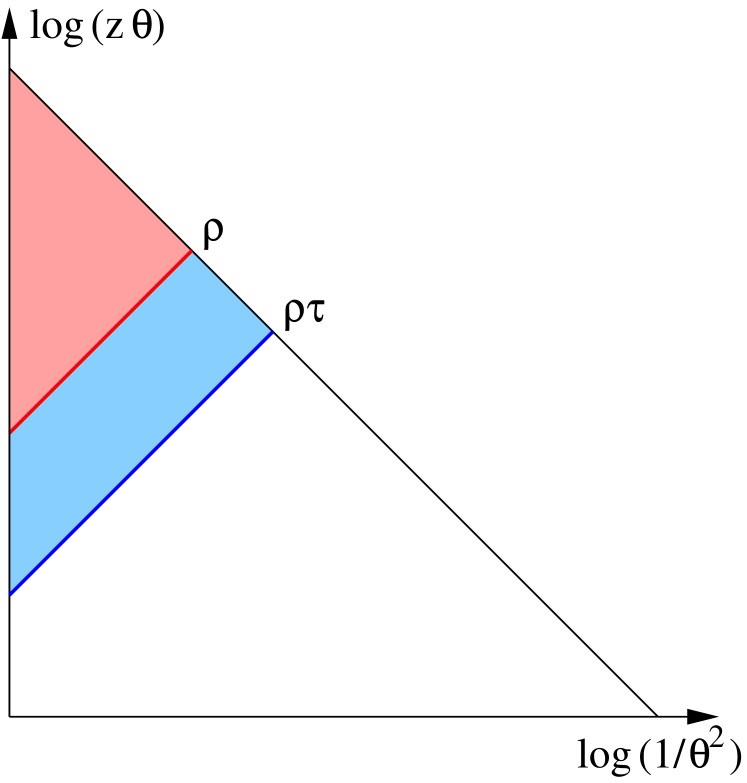
where the first line takes into account emissions from the leading parton $p_{0}$ while the second accounts for secondary gluon emissions from the first emitted gluon $p_{1}$. The arguments of the strong coupling are given as factors multiplying the “natural” scale of the problem, $p_{t}R$. The phase-space corresponding to the primary emissions is represented in Fig. 1(a).

(a) $N$-subjettiness

(b) Mass-drop

(c) Energy correlation function

Figure 1: Plots of the phase-space constraints on emissions setting the mass (in red) and the jet shape (in blue).

For simplicity, we shall only quote results with a fixed coupling approximation in the main body of the paper. Results with a proper treatment of the running-coupling corrections are presented in the Appendices. In this case, the final exponent does not depend on $z_{1}$ and we find

$$R_{\tau}^{{\rm(fixed)}}(z_{1})=\frac{\alpha_{s}C_{R}}{\pi}\left[L_{\tau}^{2}/2+L_{\rho}L_{\tau}+B_{i}L_{\tau}\right]+\frac{\alpha_{s}C_{A}}{\pi}\left[L_{\tau}^{2}/2+B_{g}L_{\tau}\right],$$ (14)

where, for quark jets, we have $C_{R}=C_{F}$ and $B_{i}=B_{q}=-3/4$ while for gluon jets we have $C_{R}=C_{A}$ and $B_{i}=B_{g}=-(11C_{A}-4n_{f}T_{R})/(12C_{A})$.

4.2 $\mu^{2}$ cut

As for the case of $N$-subjettiness, we first have to find, given the emissions $p_{1}$ and $p_{2}$ with $p_{1}$ giving the dominant contribution to the mass, what is the value of the mass-drop parameter $\mu^{2}$. Since $\mu^{2}$ is defined by undoing the last clustering step, it will depend on the jet algorithm we use to (re-)cluster the jet. The Cambridge/Aachen algorithm is a common choice but does not work here. Indeed, undoing the last step of a Cambridge/Aachen clustering would separate the emission at the largest angle from the rest of the jet, regardless of the transverse momentum of that emission. This is not infrared safe. We further discuss infrared-safety issues in Appendix C.

Instead, we shall define $\mu^{2}$ by undoing the last step of a generalised-$k_{t}$ clustering with $p=1/2$. The motivation for this is the same as the motivation for the axes choice in the previous section: the generalised-$k_{t}$ algorithm with $p=1/2$ follows closely the ordering in mass. To keep things unambiguous, we shall denote by $\mu_{p}^{2}$ the mass-drop parameter obtained by undoing the last step of a generalised-$k_{t}$ clustering with parameter $p$. The (infrared-unsafe) case of a C/A clustering would correspond to $\mu_{0}^{2}$ while we will be interested in $\mu_{1/2}^{2}$, although the calculation can be performed for any positive $p$.

Again, we leave the technical details of the calculation for Appendix B.2. In a nutshell, the hard parton and the first emission (setting the mass) will form two subjets, and the second emission, setting the subjet mass, will be clustered with whichever of these two subjets is closest. In the end, keeping in mind that, to our leading-logarithmic accuracy we can assume strong ordering in angle ($\theta_{2}\ll\theta_{1}$ or $\theta_{2}\gg\theta_{1}$), we find

$$(z_{1}\theta_{1}^{2})\mu_{1/2}^{2}\approx\begin{cases}z_{2}\theta_{2}^{2}&\text{for }\theta_{2}<\theta_{1}\text{ or }(\theta_{2}>\theta_{1}\text{ and }\theta_{2}<\theta_{12}),\\ z_{1}z_{2}\theta_{2}^{2}&\text{for }(\theta_{2}>\theta_{1}\text{ and }\theta_{2}>\theta_{12}),\\ z_{1}^{2}z_{2}\theta_{12}^{2}&\text{for secondary emissions.}\end{cases}$$ (15)

There is a crucial difference between mass-drop and $N$-subjettiness: the latter can be seen as $(1/p_{t})\sum_{\rm j\in subjets}m_{j}^{2}/p_{t,j}$ which has an extra $1/p_{t,j}$ compared to $\mu_{1/2}^{2}$. This leads to different expressions whenever the jet with the largest mass is not the one with the largest $p_{t}$. The secondary emissions and large-angle radiations will therefore give additional suppressions for $N$-subjettiness compared to the mass-drop.

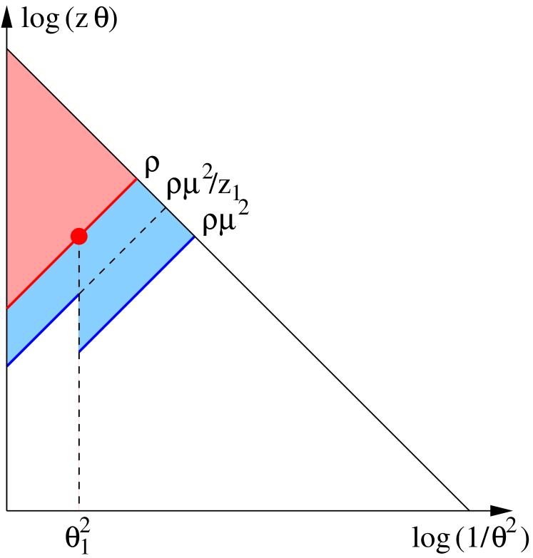
With similar arguments, it is easy to realise that additional emissions with smaller masses will not affect this calculation, so that, at leading-logarithmic accuracy, the lowest order simply exponentiates according to eq. (3). The vetoed phase-space for emissions is represented in Fig. 1(b) and we get

$$R_{\mu_{1/2}^{2}}(z_{1}) =\int_{0}^{1}\frac{d\theta_{2}^{2}}{\theta_{2}^{2}}\int_{0}^{1}dz_{2}\,\frac{\alpha_{s}(z_{2}\theta_{2})}{2\pi}\,P_{i}(z_{2})\,\bigg{\{}\Theta(\theta_{2}^{2}<\theta_{1}^{2})\,\Theta(\rho>z_{2}\theta_{2}^{2}>\rho\mu^{2})$$

$$\qquad\qquad+\Theta(\theta_{2}^{2}>\theta_{1}^{2})\Big{[}\frac{1}{2}\Theta(\rho>z_{2}\theta_{2}^{2}>\rho\mu^{2})+\frac{1}{2}\Theta(\rho>z_{2}\theta_{2}^{2}>\theta_{1}^{2}\mu^{2})\Big{]}\bigg{\}}$$

$$+\int_{0}^{\theta_{1}^{2}}\frac{d\theta_{12}^{2}}{\theta_{12}^{2}}\int_{0}^{1}dz_{2}\,\frac{\alpha_{s}(z_{1}z_{2}\theta_{12})}{2\pi}\,P_{g}(z_{2})\,\Theta(z_{1}z_{2}\theta_{12}^{2}/\theta_{1}^{2}>\mu^{2}).$$ (16)

For a fixed coupling approximation, we find

$$R_{\mu_{1/2}^{2}}^{{\rm(fixed)}}(z_{1}) =\frac{\alpha_{s}C_{R}}{\pi}\big{[}(L_{\rho}+L_{1}+L_{\mu})L_{\mu}/2+\frac{1}{2}(L_{\rho}-L_{1})(L_{\mu}-L_{1})\Theta(L_{\mu}>L_{1})+B_{i}L_{\mu}\big{]}$$

$$+\frac{\alpha_{s}C_{A}}{\pi}\left[(L_{\mu}-L_{1})^{2}/2+B_{g}(L_{\mu}-L_{1})\right]\,\Theta(L_{\mu}>L_{1}).$$ (17)

4.3 $C_{2}$ cut

For two strongly-ordered emissions $p_{1}(z_{1},\theta_{1})$ and $p_{2}(z_{2},\theta_{2})$, such that $z_{1}\theta_{1}^{2}\gg z_{2}\theta_{2}^{2}$, one finds, for primary emissions,

$$C_{2}=\frac{1}{z_{1}^{2}\theta_{1}^{4}}z_{1}z_{2}(1-z_{1}-z_{2})\theta_{1}^{2}\theta_{2}^{2}\theta_{12}^{2}\simeq\frac{z_{2}\theta_{2}^{2}}{z_{1}\theta_{1}^{2}}\,{\rm max}(\theta_{1}^{2},\theta_{2}^{2})$$ (18)

which is the same result as the one we obtained in the $N$-subjettiness case with an extra factor ${\rm max}(\theta_{1}^{2},\theta_{2}^{2})$. For secondary emissions, $\theta_{12}\ll\theta_{1}$, hence $\theta_{2}\simeq\theta_{1}$ and we have (with $z_{2}$ measuring the momentum fraction wrt emission 1)

$$C_{2}\simeq z_{2}\frac{\theta_{12}^{2}}{\theta_{1}^{2}}\theta_{1}^{2}=z_{2}\theta_{12}^{2}.$$ (19)

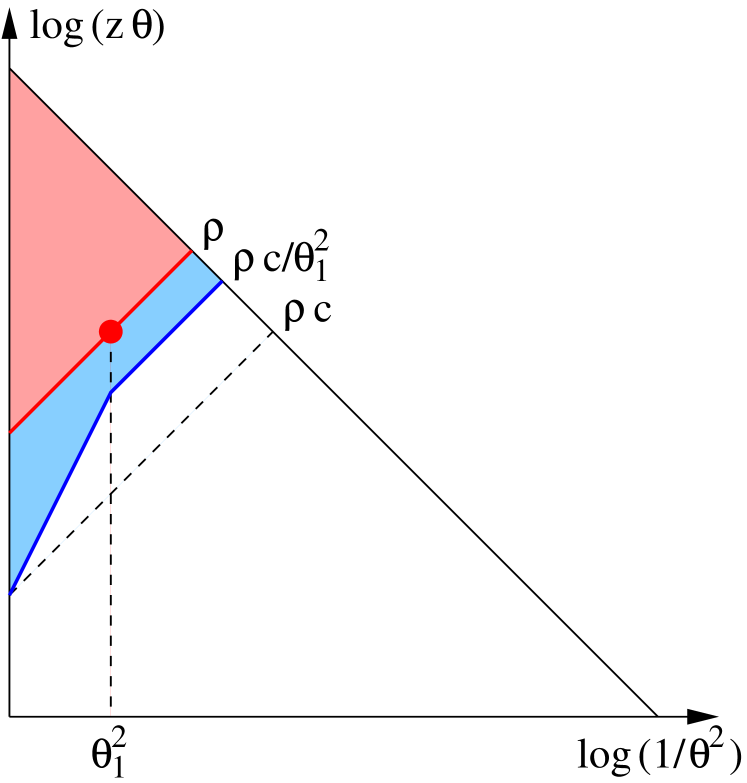
The corresponding phase-space is represented in Fig. 1(c) and gives

$$R_{C_{2}}(z_{1}) =\int_{0}^{1}\frac{d\theta_{2}^{2}}{\theta_{2}^{2}}\int_{0}^{1}dz_{2}\,\frac{\alpha_{s}(z_{2}\theta_{2})}{2\pi}\,P_{i}(z_{2})\,\Theta(\rho>z_{2}\theta_{2}^{2})$$

$$\qquad\qquad\Big{[}\Theta(\theta_{2}^{2}<\theta_{1}^{2})\,\Theta(z_{2}\theta_{2}^{2}\theta_{1}^{2}>\rho C)+\Theta(\theta_{2}^{2}>\theta_{1}^{2})\,\Theta(z_{2}\theta_{2}^{4}>\rho C)\Big{]}$$

$$+\int_{0}^{\theta_{1}^{2}}\frac{d\theta_{12}^{2}}{\theta_{12}^{2}}\int_{0}^{1}dz_{2}\,\frac{\alpha_{s}(z_{1}z_{2}\theta_{12})}{2\pi}\,P_{g}(z_{2})\,\Theta(z_{2}\theta_{12}^{2}>C).$$ (20)

For a fixed coupling approximation, one finds

$$R_{C_{2}}^{{\rm(fixed)}}(z_{1}) =\frac{\alpha_{s}C_{R}}{\pi}\big{[}L_{e}^{2}/2+(L_{e}-L_{\rho}+L_{1})(L_{1}+B_{i})\Theta(L_{e}>L_{\rho}-L_{1})\big{]}$$

$$+\frac{\alpha_{s}C_{A}}{\pi}\big{[}(L_{e}-L_{\rho}+L_{1})^{2}/2+B_{g}(L_{e}-L_{\rho}+L_{1})\big{]}\Theta(L_{e}>L_{\rho}-L_{1}).$$ (21)

If we decide to work with $D_{2}=C_{2}/\rho$ rather than $C_{2}$, and define $L_{d}=\log(1/D_{2})=L_{e}-L_{\rho}$, we get, assuming $L_{d}>0$,

$$R_{D_{2}}^{{\rm(fixed)}}(z_{1}) =\frac{\alpha_{s}C_{R}}{\pi}\big{[}(L_{d}+L_{\rho})^{2}/2+(L_{1}+L_{d})(L_{1}+B_{i})\big{]}$$

$$+\frac{\alpha_{s}C_{A}}{\pi}\big{[}(L_{d}+L_{1})^{2}/2+(L_{d}+L_{1})B_{g}\big{]}.$$ (22)

4.4 Recursive $\tau_{21}$ cut

We now move to the same calculations as above but apply the cut recursively declustering a C/A jet until the cut is met (see Sec. 2).

The calculation of the shapes mostly remains unchanged but the recursion will affect the allowed phase-space for emissions. As before, let us assume that $p_{1}(\theta_{1},z_{1})$ is the emission that dominates the mass after the recursion procedure has been applied and see what constraints on the phase-space the cut imposes on additional emissions $p_{2}(\theta_{2},z_{2})$.

For emissions at angles $\theta_{2}$ smaller than $\theta_{1}$, the de-clustering will reach $p_{1}$ before $p_{2}$, which corresponds to the same situation as for the non-recursive case. In fact it remains true for all shape variables under consideration in this paper that for such angular configurations the results from the recursive and non-recursive variants coincide.

Differences occur for emissions at angles larger than $\theta_{1}$. The physical reason for that comes from emissions at angles larger than $\theta_{1}$ and which would dominate the mass, i.e. for which $z_{2}\theta_{2}^{2}>z_{1}\theta_{1}^{2}$. In the non-recursive case, these emissions are forbidden by our constraint on the jet mass and this is included in the Sudakov suppression for the jet mass $R_{\rm mass}(\rho)$ in Eq. (3), which imposes that the mass of the jet is truly dominated by the $(z_{1},\theta_{1}^{2})$ emission. In the situation where the cut on the shape is applied recursively, some extra care is needed since some of these emissions — that are vetoed in the non-recursive case because they would lead to a larger jet mass — can be simply discarded by the recursive procedure. In such a case, they should no longer be forbidden.

For the large-angle region, $\theta_{2}>\theta_{1}$ we therefore have to separate 4 different regions:

• for $z_{2}\theta_{2}^{2}<\rho\tau$, we have $\tau_{21}\approx z_{2}\theta_{2}^{2}/z_{1}\theta_{1}^{2}=z_{2}\theta_{2}^{2}/\rho<\tau$, meaning that the constraint is satisfied. That region is therefore allowed,

• for $\rho\tau<z_{2}\theta_{2}^{2}<\rho$, we have $\tau_{21}\approx z_{2}\theta_{2}^{2}/z_{1}\theta_{1}^{2}=z_{2}\theta_{2}^{2}/\rho$ as in the previous case, but this time it does not satisfy the condition $\tau_{21}<\tau$. The emission $(z_{2},\theta_{2}^{2})$ will thus be discarded, meaning that this region is again allowed,

• for $\rho<z_{2}\theta_{2}^{2}<\rho/\tau$, we now have $\tau_{21}\approx z_{1}\theta_{1}^{2}/z_{2}\theta_{2}^{2}=\rho/z_{2}\theta_{2}^{2}$, i.e. $\tau_{21}>\tau$. The condition is once again not satisfied and the region is allowed.

• for $z_{2}\theta_{2}^{2}>\rho/\tau$, we find similarly $\tau_{21}\approx z_{1}\theta_{1}^{2}/z_{2}\theta_{2}^{2}=\rho/z_{2}\theta_{2}^{2}<\tau$. The condition on $\tau_{21}$ would be met, leaving a jet with a mass $z_{2}\theta_{2}^{2}>\rho$. This region is therefore forbidden.

Compared to the non-recursive case, the vetoed region at large angle is therefore reduced.

In the above discussion, we tacitly assumed that we were working with the gen-$k_{t}(1/2)$ axes or with the optimal axes, but the argument is more general. We could also define $\tau_{21}$ using the exclusive C/A axes, automatically available from the declustering procedure. Indeed, in that case, all emissions with $z_{2}\theta_{2}^{2}<\rho/\tau$ would fail the cut on $\tau_{21}$ and be discarded. We will come back to that point later on.

(a) $N$-subjettiness or mass-drop

(b) Energy-correlation function

Figure 2: Same as Fig. 1 but this time for cases where the cut is applied recursively.

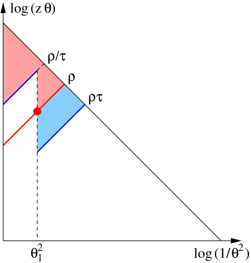
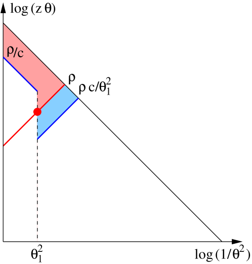
Again, the lowest order result simply exponentiates and the Sudakov suppression, depicted in Fig. 2(a) is

$$R_{\tau,\rm rec}(z_{1}) =\int_{0}^{1}\frac{d\theta_{2}^{2}}{\theta_{2}^{2}}\int_{0}^{1}dz_{2}\,\frac{\alpha_{s}(z_{2}\theta_{2})}{2\pi}\,P_{i}(z_{2})\,\big{[}\Theta(\theta_{2}^{2}>\theta_{1}^{2})\,\Theta(z_{2}\theta_{2}^{2}>\rho/\tau)$$

$$\phantom{=\int_{0}^{1}\frac{d\theta_{2}^{2}}{\theta_{2}^{2}}\int_{0}^{1}dz_{2}\,\frac{\alpha_{s}(z_{2}\theta_{2})}{2\pi}\,P_{i}(z)}+\Theta(\theta_{2}^{2}<\theta_{1}^{2})\,\Theta(z_{2}\theta_{2}^{2}>\rho\tau)\big{]}$$

$$+\int_{0}^{\theta_{1}^{2}}\frac{d\theta_{12}^{2}}{\theta_{12}^{2}}\int_{0}^{1}dz_{2}\,\frac{\alpha_{s}(z_{1}z_{2}\theta_{2})}{2\pi}\,P_{g}(z_{2})\,\Theta(z_{2}\theta_{12}^{2}/\theta_{1}^{2}>\tau)-R_{\rm mass}(\rho),$$ (23)

where we have subtracted $R_{\rm mass}(\rho)$ which has already been included in (3).

For a fixed coupling approximation, this gives

$$R_{\tau,\rm rec}^{{\rm(fixed)}}(z_{1}) =\frac{\alpha_{s}C_{R}}{\pi}\Big{\{}\left[L_{\tau}^{2}/2-L_{\rho}L_{\tau}+2L_{1}L_{\tau}+B_{i}L_{\tau}\right]\,\Theta(L_{\tau}<L_{1})$$

$$\phantom{=\frac{\alpha_{s}C_{F}}{\pi}}+\left[L_{\tau}^{2}-L_{\rho}L_{\tau}+L_{1}L_{\tau}+L_{1}^{2}/2+B_{i}L_{1}\right]\,\Theta(L_{1}<L_{\tau}<L_{\rho})$$

$$\phantom{=\frac{\alpha_{s}C_{F}}{\pi}}+\Big{[}\frac{1}{2}(L_{\rho}+L_{1}+L_{\tau}+2B_{i})(L_{\tau}+L_{1}-L_{\rho})\Big{]}\,\Theta(L_{\rho}<L_{\tau})\Big{\}}$$

$$+\frac{\alpha_{s}C_{A}}{\pi}\left[L_{\tau}^{2}/2+B_{g}L_{\tau}\right].$$ (24)

4.5 Recursive $\mu^{2}$ cut (pure mass-drop tagger)

The situation is mostly the same as for the recursive $\tau_{21}$ cut. Here, the use of a recursive criterion allows to use either the subjets naturally given by the C/A declustering or the gen-$k_{t}(1/2)$ subjets. The results presented in this section are valid for both $\mu_{0}^{2}$ and $\mu_{1/2}^{2}$, although, as we will see in the next paragraph, different axes choice yield the same answer for the mass distribution in different ways, and would give different answers for other observables.

As before, for $\theta_{2}$ smaller than $\theta_{1}$, the declustering has no effect and the results are as obtained in Sec. 4.2. The complication related to the clustering distance for $\theta_{2}\gg\theta_{1}$ is absent here because of the declustering, and only emissions with $z_{2}\theta_{2}^{2}>\rho/\mu^{2}$ have to be vetoed. In all other cases, either the mass-drop condition fails and the emission is simply discarded, or the mass-drop condition is satisfied but the mass of the jet remains $z_{1}\theta_{1}^{2}$. E.g., for the natural choice, $\mu_{0}^{2}$, all emissions in the region $z_{2}\theta_{2}^{2}<\rho/\mu_{0}^{2}$ will fail the condition and be discarded before the recursion continues. That said, the only remaining difference between a recursive $\mu^{2}$ cut and a recursive $\tau_{21}$ cut will be in the extra factor $z_{1}$ in the secondary emissions (see, e.g. Sec. 4.2) and we find

$$R_{\mu^{2},\rm rec}(z_{1}) =\int_{0}^{1}\frac{d\theta_{2}^{2}}{\theta_{2}^{2}}\int_{0}^{1}dz_{2}\,\frac{\alpha_{s}(z_{2}\theta_{2})}{2\pi}\,P_{i}(z_{2})\,\big{[}\Theta(\theta_{2}^{2}>\theta_{1}^{2})\,\Theta(z_{2}\theta_{2}^{2}>\rho/\mu^{2})$$

$$\phantom{=\int_{0}^{1}\frac{d\theta_{2}^{2}}{\theta_{2}^{2}}\int_{0}^{1}dz_{2}\,\frac{\alpha_{s}(z_{2}\theta_{2})}{2\pi}\,P_{i}(z)}+\Theta(\theta_{2}^{2}<\theta_{1}^{2})\,\Theta(z_{2}\theta_{2}^{2}>\rho\mu^{2})\big{]}$$

$$+\int_{0}^{\theta_{1}^{2}}\frac{d\theta_{12}^{2}}{\theta_{12}^{2}}\int_{0}^{1}dz_{2}\,\frac{\alpha_{s}(z_{1}z_{2}\theta_{2})}{2\pi}\,P_{g}(z_{2})\,\Theta(z_{1}z_{2}\theta_{12}^{2}/\theta_{1}^{2}>\mu^{2})-R_{\rm mass}(\rho).$$ (25)

For a fixed coupling approximation, we get

$$R_{\mu^{2},\rm rec}^{{\rm(fixed)}}(z_{1}) =\frac{\alpha_{s}C_{R}}{\pi}\Big{\{}\left[L_{\mu}^{2}/2-L_{\mu}L_{\rho}+2L_{\mu}L_{1}+B_{i}L_{\mu}\right]\,\Theta(L_{\mu}<L_{1})$$

$$\phantom{=\frac{\alpha_{s}C_{F}}{\pi}}+\left[L_{\mu}^{2}-L_{\mu}L_{\rho}+L_{\mu}L_{1}+L_{1}^{2}/2+B_{i}L_{1}\right]\,\Theta(L_{1}<L_{\mu}<L_{\rho})$$

$$\phantom{=\frac{\alpha_{s}C_{F}}{\pi}}+\Big{[}\frac{1}{2}(L_{\rho}+L_{1}+L_{\mu}+2B_{i})(L_{\mu}+L_{1}-L_{\rho})\Big{]}\,\Theta(L_{\rho}<L_{\mu})\Big{\}}$$

$$+\frac{\alpha_{s}C_{A}}{\pi}\left[(L_{\mu}-L_{1})^{2}/2+B_{g}(L_{\mu}-L_{1})\right]\,\Theta(L_{\mu}>L_{1}),$$ (26)

where the $C_{R}$ contribution is the same as for the recursive $\tau_{21}$ cut and the $C_{A}$ contribution is the same as for the non-recursive $\mu_{1/2}^{2}$ cut.

4.6 Recursive $C_{2}$ cut

Again, the calculation unfolds as for the two recursive cases above with a contribution from “failed” conditions for $\theta_{2}>\theta_{1}$ and a standard constraint for $\theta_{2}<\theta_{1}$. In the first case, $e_{2}$ (resp. $e_{3}$) is set by emission $p_{2}$ (resp. $p_{1}$) and $\theta_{12}\approx\theta_{2}$. In the second case, $e_{2}$ (resp. $e_{3}$) is set by emission $p_{1}$ (resp. $p_{2}$) and $\theta_{12}\approx\theta_{1}$, yielding

$$C_{2}=\frac{z_{1}\theta_{1}^{2}}{z_{2}}\Theta(\theta_{2}>\theta_{1})+\frac{z_{2}\theta_{2}^{2}}{z_{1}}\Theta(\theta_{2}<\theta_{1}).$$ (27)

The Sudakov exponent will ultimately be given by

$$R_{C,\rm rec}(z_{1}) =\int_{0}^{1}\frac{d\theta_{2}^{2}}{\theta_{2}^{2}}\int_{0}^{1}dz_{2}\,\frac{\alpha_{s}(z_{2}\theta_{2})}{2\pi}\,P_{i}(z_{2})\,\big{[}\Theta(\theta_{2}^{2}>\theta_{1}^{2})\,\Theta(z_{2}\theta_{2}^{2}>z_{1}\theta_{1}^{2})\,\Theta(z_{2}>\rho/C)$$

$$\phantom{=\int_{0}^{1}\frac{d\theta_{2}^{2}}{\theta_{2}^{2}}\int_{0}^{1}dz_{2}\,\frac{\alpha_{s}(z_{2}\theta_{2})}{2\pi}}+\Theta(\theta_{2}^{2}<\theta_{1}^{2})\,\Theta(z_{2}\theta_{2}^{2}>z_{1}\theta_{1}^{2})$$

$$\phantom{=\int_{0}^{1}\frac{d\theta_{2}^{2}}{\theta_{2}^{2}}\int_{0}^{1}dz_{2}\,\frac{\alpha_{s}(z_{2}\theta_{2})}{2\pi}}+\Theta(\theta_{2}^{2}<\theta_{1}^{2})\,\Theta(z_{2}\theta_{2}^{2}<z_{1}\theta_{1}^{2})\,\Theta(z_{2}\theta_{2}^{2}>\rho C/\theta_{1}^{2})\big{]}$$

$$+\int_{0}^{\theta_{1}^{2}}\frac{d\theta_{12}^{2}}{\theta_{12}^{2}}\int_{0}^{1}dz_{2}\,\frac{\alpha_{s}(z_{1}z_{2}\theta_{2})}{2\pi}\,P_{g}(z_{2})\,\Theta(z_{2}\theta_{12}^{2}>C)-R_{\rm mass}(\rho).$$ (28)

For a fixed coupling approximation, we obtain

$$R_{C,\rm rec}^{{\rm(fixed)}}(z_{1}) =\frac{\alpha_{s}C_{R}}{\pi}\Big{\{}\left[-L_{e}^{2}/2\right]\,\Theta(L_{e}<L_{\rho}-L_{1})$$ (29)

$$\phantom{=}+\left[(L_{v}+L_{1}-L_{\rho})(L_{v}+2L_{1}-L_{\rho}+B_{i})-L_{e}^{2}/2\right]\,\Theta(0<L_{\rho}-L_{e}<L_{1})$$

$$\phantom{=}+\left[(L_{e}+2L_{1}-2L_{\rho})(L_{e}+2L_{1})/2+B_{i}(L_{e}-2L_{\rho}+2L_{1})\right]\,\Theta(L_{e}>L_{\rho})\Big{\}}$$

$$+\frac{\alpha_{s}C_{A}}{\pi}\left[(L_{e}+L_{1}-L_{\rho})^{2}/2+B_{g}(L_{e}+L_{1}-L_{\rho})\right]\,\Theta(L_{e}>L_{\rho}-L_{1}).$$

4.7 Towards NLL accuracy

In this article, as we have stated before, we are aiming to achieve only a (modified) leading-logarithmic description of the shape variables we study here. This level of approximation has already been demonstrated to capture the main physical features of various jet tagging and grooming tools (see e.g. Refs. Dasgupta:2013ihk ; Dasgupta:2013via ).

Nevertheless it may ultimately prove important to extend the scope of our current studies in various directions. One potential reason for this could be that here we study tools that have some broad similarities e.g. all of them place constraints on subjet masses. In order to understand in more detail the differences between these tools it would be helpful to increase the accuracy of our analytical predictions, so that differences that may arise beyond LL effects are effectively highlighted. We would also expect such differences to show up in the Monte Carlo event generator studies, like those carried out below, since event generators would partially capture many sources of subleading corrections.

Secondly we do not study here the question of optimal values of cuts on subjet variables, mainly confining ourselves to the region with both $v_{\rm cut}$ and $\rho\ll 1$. To meaningfully explore the dependence on $v_{\rm cut}$ and $\rho$ over a broader range of values of the variables concerned, one may need to carefully investigate effects beyond leading-logarithmic level including the role of hard non-logarithmically enhanced contributions.

With such future developments in mind we discuss below several extra ingredients that are required to reach NLL accuracy: soft-and-large-angle contributions, multiple emissions, the two-loop $\beta$ function for $\alpha_{s}$, finite $z_{1}$ corrections and non-global logarithms Dasgupta:2001sh .

For the figures where we compare to Monte Carlo simulations, we will include multiple emission effects (numerically important; see below for their effect on the radiator function), two-loop running coupling corrections (trivial to add, see Appendix A.1) as well as finite $z_{1}$ corrections (important for the physics discussion; see Appendix A.4).

We have not included in our analytic results contributions which are power-suppressed in the jet radius $R$. Although they would be relevant for a full phenomenological prediction, and can be substantial at the peak of the distributions (see e.g. Section 5 of Dasgupta:2012hg ), these are expected to have little impact when comparing the discriminative power of different jet shapes. Moreover, they would be further reduced by the combination with a grooming procedure which, as we argue in Section 6, is the natural future direction of this work.

Soft-and-large-angle radiation.

A source of single-logarithmic corrections comes from radiating soft gluons at large angles. This would correspond to all the limits beyond the strict collinear ordering that we have adopted until now i.e. it can come from either $\theta_{1}\sim R$, or $\theta_{2}\sim R$, or $\theta_{1}\sim\theta_{2}$.

The first two regions would give single-logarithmic corrections proportional to $R^{2}$. In the small-$R$ approximation we have adopted so far, these would further be suppressed. At the same order of accuracy, one would also have to include contributions coming from initial-state radiation and potential colour-correlation with the recoiling partonic system Dasgupta:2012hg . Taking these into account would also add single-logarithmic contributions to the mass distributions. This significantly complicates the discussion, especially for signal jets, where the mass would no longer be identical to the boosted heavy-boson mass and we would have to impose a certain window around the signal mass. In practice, therefore, one usually applies these techniques together with some grooming procedure which would drastically change this discussion. Some first results have already been obtained in Dasgupta:2015yua for grooming techniques and we reserve for future work the addition of radiation constraints to that discussion. We will comment on that a bit further in Section 6.

The situation for $\theta_{1}\sim\theta_{2}$ is a bit more involved and we show in Appendix D that it would only contribute to single-logarithmic corrections suppressed by $\theta_{1}^{2}$. These contributions are also at most proportional to $R^{2}$, although since radiation constraints tend to take most of their discriminative power from the large-angle region $\theta_{2}>\theta_{1}$, it makes sense to consider a region $\theta_{1}\ll R$. In that case, the contribution from the $\theta_{1}\sim\theta_{2}$ region would be even further suppressed.

Multiple emissions.

Multiple gluon emissions also bring single-logarithmic corrections to our results and we briefly discuss below how to account for them for the non-recursive variants of the shapes.

They correspond to cases where several gluon emissions, $(z_{2},\theta_{2}),\dots,(z_{n},\theta_{n})$, are only strongly ordered in angle and give similar contributions to the shape $v$, i.e. when $v(z_{2},\theta_{2}^{2};z_{1},\theta_{1}^{2})\sim\dots\sim v(z_{n},\theta_{n}^{2};z_{1},\theta_{1}^{2})$. This will come with a single-logarithmic correction $\alpha_{s}^{n-1}L_{v}^{n-1}$ to the resummed exponent $R$.

It is important to realise that we will keep working in the $v\ll 1$ limit and so neglect the contribution where all the $z_{i}\theta_{i}^{2}$, $i\geq 2$, are of the same order as $z_{1}\theta_{1}^{2}$. This would also give a single logarithmic correction of the form $\alpha_{s}^{n}L_{\rho}^{n}f_{n}(v)$. Up to power corrections, we can take $f_{n}$ constant and this correction would therefore simply be equivalent to the multiple-emission correction to the plain jet mass, cancelling against the corresponding normalisation in the spectrum of $v$. So, from now on, we focus on the region where all the $z_{i}\theta_{i}^{2}$, $i\geq 2$, are much smaller than $z_{1}\theta_{1}^{2}$ and compute the corresponding correction to $R_{v}(z_{1})$ for a fixed $z_{1}$.

The case of $N$-subjettiness and energy-correlation functions are mostly straightforward. In the kinematical configurations under consideration, the (optimal or gen-$k_{t}$) $N$-subjettiness axes will still align with the jet axis and with the emission $(z_{1},\theta_{1})$ setting the mass. At a given $z_{1}$, both $\tau_{21}$ and $C_{2}$ will therefore be additive and the correction to $R_{v}(z_{1})$ will be $\gamma_{E}R_{v}^{\prime}(z_{1})+\log[\Gamma(1+R_{v}^{\prime}(z_{1}))]$ where $\gamma_{E}$ is the Euler constant and $R_{v}^{\prime}(z_{1})$ is the derivative of $R_{v}(z_{1})$ wrt $L_{v}$.

The situation is a bit more involved for the mass drop parameter. Had we defined $\mu^{2}$ as $(m_{j_{1}}^{2}+m_{j_{2}}^{2})/m^{2}$, $\mu^{2}$ would have been additive and the similar conclusion as for $\tau_{21}$ and $C_{2}$ would have been reached. Since $\mu^{2}$ is defined as a maximum over the two subjets rather than a sum, we should instead use the fact that the condition $\mu^{2}<\mu_{\rm cut}^{2}$ will be satisfied if both $m_{j_{1}}^{2}<\mu^{2}m^{2}$ and $m_{j_{2}}^{2}<\mu^{2}m^{2}$.

In practice, the emissions will either be clustered with the original hard parton or with the emission setting the mass. How exactly the particles in the jet are sifted in these two sets can depend non-trivially on the details of the clustering. If we take as an approximation, the assumption that particles behave independently, they will be clustered with the hard parton or the emission setting the mass according to which is geometrically closer, in a way similar to the heavy-jet mass in $e^{+}e^{-}$ collisions Catani:1991bd . If we split $R_{\mu_{1/2}^{2}}(z_{1})$ in two contributions according to whether the emissions are clustered with one or the other of the subjets,

$$R_{\mu_{1/2}^{2},0}(z_{1}) =\int_{0}^{1}\frac{d\theta_{2}^{2}}{\theta_{2}^{2}}\int_{0}^{1}dz_{2}\,\frac{\alpha_{s}(z_{2}\theta_{2})}{2\pi}\,P_{i}(z_{2})\,\big{[}\Theta(\theta_{2}^{2}<\theta_{1}^{2})\,\Theta(\rho>z_{2}\theta_{2}^{2}>\rho\mu^{2})$$

$$\phantom{=\int_{0}^{1}\frac{d\theta_{2}^{2}}{\theta_{2}^{2}}\int_{0}^{1}dz_{2}\,\frac{\alpha_{s}(z_{2}\theta_{2})}{2\pi}P_{i}(z_{2})}+\frac{1}{2}\Theta(\theta_{2}^{2}>\theta_{1}^{2})\Theta(\rho>z_{2}\theta_{2}^{2}>\rho\mu^{2})\big{]}$$ (30)

and

$$R_{\mu_{1/2}^{2},1}(z_{1}) =\int_{0}^{1}\frac{d\theta_{2}^{2}}{\theta_{2}^{2}}\int_{0}^{1}dz_{2}\,\frac{\alpha_{s}(z_{2}\theta_{2})}{2\pi}\,P_{i}(z_{2})\Theta(\theta_{2}^{2}>\theta_{1}^{2})\frac{1}{2}\Theta(\rho>z_{2}\theta_{2}^{2}>\theta_{1}^{2}\mu^{2})$$

$$+\int_{0}^{\theta_{1}^{2}}\frac{d\theta_{12}^{2}}{\theta_{12}^{2}}\int_{0}^{1}dz_{2}\,\frac{\alpha_{s}(z_{1}z_{2}\theta_{12})}{2\pi}\,P_{g}(z_{2})\,\Theta(z_{1}z_{2}\theta_{12}^{2}/\theta_{1}^{2}>\mu^{2}).$$ (31)

each of these two parts become additive and we obtain the following correction to $R_{\mu_{1/2}^{2}}$

$$\gamma_{E}R_{\mu_{1/2}^{2}}^{\prime}(z_{1})+\log[\Gamma(1+R_{\mu_{1/2}^{2},0}^{\prime}(z_{1}))]+\log[\Gamma(1+R_{\mu_{1/2}^{2},1}^{\prime}(z_{1}))].$$ (32)

This is however only an approximation and we leave a more precise treatment for future work. At this stage, it can also be seen as the fact that, compared to $N$-subjettiness and energy-correlation functions, the mass-drop parameter is more delicate to tackle analytically.

Before going to comparisons with Monte Carlo simulations, we can observe that the two axes of $2$-subjettiness can be viewed as partitioning the jet in two subjets, one with the jet constituents closer to the hard parton, one with those closer to the emission setting the mass. If instead of summing over all particles in the jet we were summing independently over the contributions of each of the two subjets and defining a modified $2$-subjettiness as the maximum of these two contributions, the resummation of multiple emissions for that observable would follow Eq. (32). However, since $\Gamma(1+R_{0}^{\prime})\Gamma(1+R_{1}^{\prime})/\Gamma(1+R_{0}^{\prime}+R_{1}^{\prime})<1$ we should expect this variant of $2$-subjettiness to perform worse than its original definition. Conversely, defining the mass-drop parameter as $(m_{j_{1}}^{2}+m_{j_{2}}^{2})/m_{j}^{2}$ would not only make its analytic behaviour simpler but could also translate into a slightly more efficient tool.

Two-loop running coupling.

The inclusion of the two-loop $\beta$ function is purely a technical complication. In the results presented in Appendix A, we have included their effects.

Finite $z_{1}$ corrections.

Finite $z_{1}$ corrections would typically give contributions to $R(z_{1})$ like $\alpha_{s}\log(1/v)\log(1/z_{1})$ or $\alpha_{s}\log(1/v)\log(1/(1-z_{1}))$. The first of these two terms, integrated over the $1/z_{1}$ part of the splitting function corresponding to the first emission, will give a double-logarithmic contribution that we already have included. The second term, as well as the first term integrated over the non-singular contributions to the $P(z_{1})$ splitting function will become important at NLL accuracy. Indeed, after integration over $z_{1}$, they would give corrections proportional to $\alpha_{s}L_{v}$ which contribute at the single-log accuracy. To properly include these corrections, it is sufficient to integrate over the full $P(z_{i})$ splitting function (rather than just including the finite piece as a $B_{i}$ term) and to keep the full $z_{1}$ dependence when we calculate the shapes in order to get single-logarithmic corrections to $R(z_{1})$.

The corresponding results are presented in Appendix A.4. It is interesting to note that their calculation allows for a nice physical discussion of similarities and differences between background and signal jets. Unless explicitly mentioned, these results will be used for the figures in this paper.

Non-global logarithms.

Non-global logarithms are known to be difficult contributions to handle, especially if we want to go beyond the large-$N_{c}$ approximation, where a general treatment is still lacking. We will not provide an explicit calculation of their contribution in this paper. We note however that it might be beneficial to apply grooming techniques such as SoftDrop which are known to eliminate the contributions from non-global logarithms.

4.8 Comparison with fixed-order Monte-Carlo

As a partial cross-check of our results, the expressions obtained above can be expanded in a series in $\alpha_{s}$ and compared to EVENT2 Catani:1996vz ; event2 simulations. Here we compare the (non-recursive) $\tau_{21}$, $\mu_{1/2}^{2}$ and $C_{2}$ distributions at order $\alpha_{s}$.

Note that since we are using the $N$-subjettiness implementation from FastJet contrib, we have to use $pp$ coordinates (transverse momentum, rapidity and azimuth) rather than $e^{+}e^{-}$ ones (energy and polar coordinates). To maximise the efficiency and provide quark jets with a monochromatic $p_{t}$, events are rotated so that their original $2\to 2$ scattering gives 2 jets at $y=0$. After that rotation, jets are reconstructed with the standard ($pp$) anti-$k_{t}$ algorithm antikt with $R=0.4$.

On the analytic side, we take the fixed-order results, expand (8) to first order in $\alpha_{s}$, and perform the $z_{1}$ integration.

For $N$-subjettiness, starting from (14) we get

$$\tau\,\frac{d\Sigma(\tau)}{d\tau}=\frac{\alpha_{s}C_{F}}{\pi}(L_{\rho}+L_{\tau}+B_{q})+\frac{\alpha_{s}C_{A}}{\pi}(L_{\tau}+B_{g}).$$ (33)

For the mass-drop parameter, we use (4.2) and reach

$$\mu^{2}\,\frac{d\Sigma(\mu^{2})}{d\mu^{2}} \overset{L_{\mu}<L_{\rho}}{=}\frac{1}{L_{\rho}+B_{q}}\Big{[}\frac{\alpha_{s}C_{F}}{4\pi}\big{(}3L_{\rho}^{2}+6L_{\rho}L_{\mu}-L_{\mu}^{2}+4B_{q}(2L_{\rho}+L_{\mu})+4B_{q}^{2}\big{)}$$

$$\phantom{\overset{L_{\mu}<L_{\rho}}{=}\frac{1}{L_{\rho}+B_{q}}}+\frac{\alpha_{s}C_{A}}{2\pi}\big{(}L_{\mu}^{2}+2B_{q}L_{\mu}+2B_{g}(L_{\mu}+B_{q})\big{)}\Big{]}$$

$$\overset{L_{\mu}>L_{\rho}}{=}\frac{1}{L_{\rho}+B_{q}}\Big{[}\frac{\alpha_{s}C_{F}}{\pi}\big{(}L_{\rho}^{2}+L_{\rho}L_{\mu}+B_{q}(2L_{\rho}+L_{\mu})+B_{q}^{2}\big{)}$$

$$\phantom{\overset{L_{\mu}<L_{\rho}}{=}\frac{1}{L_{\rho}+B_{q}}}+\frac{\alpha_{s}C_{A}}{2\pi}\big{(}2L_{\mu}L_{\rho}-L_{\rho}^{2}+2B_{q}L_{\mu}+2B_{g}(L_{\rho}+B_{q})\big{)}\Big{]}.$$ (34)

Finally, for the energy correlation function, we start from (4.3) and obtain

$$C_{2}\,\frac{d\Sigma(C_{2})}{dC_{2}} \overset{L_{e}<L_{\rho}}{=}\frac{1}{L_{\rho}+B_{q}}\Big{[}\frac{\alpha_{s}C_{F}}{2\pi}L_{e}(4L_{\rho}-L_{e}+4B_{q})+\frac{\alpha_{s}C_{A}}{2\pi}L_{e}(L_{e}+2B_{g})\Big{]}$$ (35)

$$\overset{L_{e}>L_{\rho}}{=}\frac{\alpha_{s}C_{F}}{2\pi}\Big{(}2L_{e}+L_{\rho}+B_{q}\frac{L_{\rho}+2B_{q}}{L_{\rho}+B_{q}}\Big{)}+\frac{\alpha_{s}C_{A}}{2\pi}\Big{(}2L_{e}-L_{\rho}+2B_{g}-B_{q}\frac{L_{\rho}}{L_{\rho}+B_{q}}\Big{)}.$$

Figure 3: Distributions for the (non-recursive) shapes at order $\alpha_{s}$ for a few specific bins in the jet mass. A constant factor $\alpha_{s}/(2\pi)$ has been factored out of the cross-section. The top row shows the distributions themselves, with solid lines corresponding to EVENT2 simulations and dashed lines to our analytic calculation. The bottom row show the difference between the two.

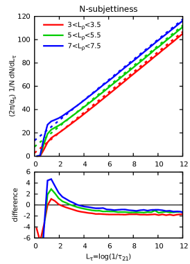
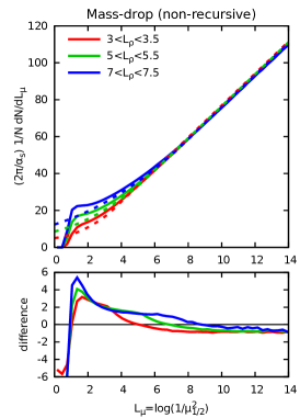
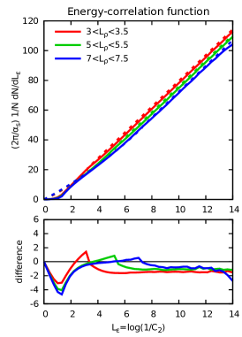
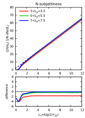
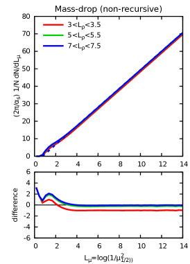
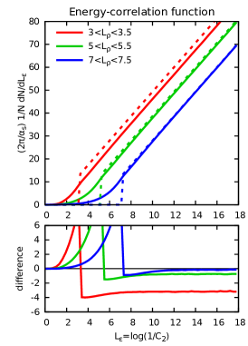
The comparison with EVENT2 is presented in Fig. 3 where we have plotted the shape distributions at order $\alpha_{s}$ together with our analytic prediction. In these plots, a constant factor $\alpha_{s}/(2\pi)$ has been factored out. From Fig. 3, we see that this difference goes at least to a constant at large $L_{v}$, meaning that we do control the leading logarithmic behaviour.

Figure 4: Coefficients of the $L_{v}$ (top row) and constant (bottom row) terms extracted from the distributions in different bins of the jet mass. For each distribution, we have separated the results in the different colour channels. In all cases, a factor $\alpha_{s}/(2\pi)$ has been factored out of the numbers that are shown.

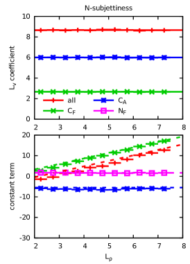
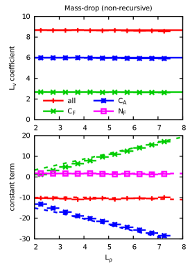
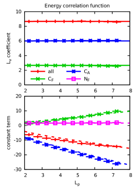
In principle, one can also wonder if the constant term can be obtained from an analytic calculation, which is, strictly speaking, beyond our leading-logarithmic accuracy. For example, we have included in equations (33)-(35) corrections coming from the hard part of the splitting function. However, we have neglected large-angle contributions proportional to $R^{2}$ and expected to be small for $R=0.4$, as well as possible finite $z_{1}$ corrections. It is unclear from Fig. 3 whether or not this fully accounts from the apparent constant value observed at large $L_{v}$. In this respect, it is also interesting to note that, contrary to the jet mass where besides the logarithmic and constant terms we would only have power corrections, the constant term in the $L_{v}$ expansion has some corrections proportional to $1/L_{\rho}$, coming from the normalisation of the shape distributions by the jet mass cross-section (see Eq. (8)). These terms can make the convergence slower.

To extract more precise information, we have fitted, in each bin of the jet mass, the coefficient of $L_{v}$ and the constant term. This has been done in each colour channel and reported in Fig. 4. Again, we see a good agreement for the linear rise with $L_{v}$ as well as for the constant terms proportional to $C_{A}$ and $N_{f}$. The slow convergence of the $C_{F}$ term is related to the above discussion.

More precise statements would require going to larger values of $L_{v}$ and $L_{\rho}$. This is difficult to explore due to limited machine precision.

4.9 Comparison with parton-shower Monte-Carlo

Our resummed analytic results can be directly compared to parton-shower Monte Carlo event generators such as Pythia pythia or Herwig herwig . To do this, we have generated QCD dijet events in 14 TeV $pp$ collisions simulated with Pythia. We have selected anti-$k_{t}$(R=1) jets with a transverse momentum of at least 3 TeV.

For our analytical predictions, we have used the results from Appendix A.4, which, unless explicitly mentioned otherwise, include all the computed global NLL corrections discussed in Section 4.7. We have fixed $\alpha_{s}(M_{z})=0.1185$ with $N_{f}=5$ and frozen the coupling at $\mu_{fr}=1$ GeV.

Figure 5: Distributions obtained from quark jets for each of the three shapes studies. Left: results obtained with Pythia including only final-state radiation (we used $p_{t,\rm jet}>3$ TeV, and $4<L_{\rho}<4.5$); right: results of our analytic calculations (for $p_{t}=3$ TeV and $L_{\rho}=4.25$).

Figure 6: Ratio of the mass spectrum obtained with a cut on one of the shapes, divided by the plain jet mass spectrum. The solid lines are obtained imposing a fixed cut on the jet, while the dashed lines are obtained by imposing the cut recursively. Left: results obtained with Pythia including only final-state radiation (we used $p_{t,\rm jet}>3$ TeV, and $L_{v}>2.4$ corresponding to $v<0.09$); right: results of our analytic calculations (for $p_{t}=3$ TeV). Note that multiple emissions are not included in these expressions since they have not been computed for the recursive versions.

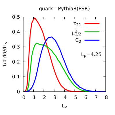
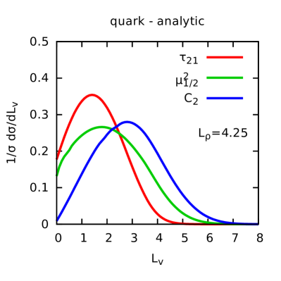
In Fig. 5, we compare the analytic results obtained for the distribution of $N$-subjettiness, the mass-drop parameter and the energy-correlation functions, at a given jet mass, with the same distributions obtained with Pythia at parton-level, including only final-state radiation. First of all, if we look at the large $L_{v}$ region, where our analytic description is valid, we see that it does reproduce nicely the Pythia simulations. However, at smaller $L_{v}$, Pythia tends to produce more peaked distributions than what we obtain analytically. In any case, the main message that one has to take from this comparison is that the generic ordering between the different shapes is well captured by our analytic calculations.

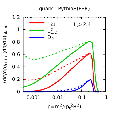
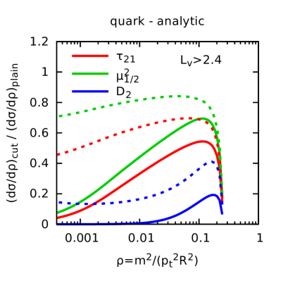
Instead of plotting the distributions themselves, we can instead look at the mass distributions. This has the advantage that we can also consider the recursive versions of the cuts on the shapes. In Fig. 6, we plotted the ratio of the mass distribution obtained after a given cut, $L_{v}>2.4$, applied recursively (dashed lines) or not (solid lines) on our three shapes, divided by the jet mass distribution without applying any cut. Globally, our analytic calculations tends to reproduce the main features of the Monte Carlo simulations, although they show longer tails at small masses. Note that for these plots, we have used $D_{2}$ instead of $C_{2}$ since, compared to the latter, the former peaks at values of $L_{v}$ closer to the other two shapes. Furthermore, since we have not computed multiple-emission corrections for the recursive versions of the shape constraints, we have also left aside the multiple-emission corrections to the non-recursive versions for the analytic results plotted in Fig. 6. It is interesting to notice that including the multiple-emission corrections for the non-recursive shapes tends to reduce the tails towards small mass, bringing more resemblance to the Pythia results. We could expect a similar behaviour for the corresponding recursive versions.

Figure 7: As a function of the jet mass, value of the cut on a given shape, $\log(1/v_{\rm cut})$ which would correspond to a 25% tagging rate. Results correspond to dijet events obtained with Pythia with $p_{t,\rm jet}>3$ TeV. The various curves correspond to different levels of the simulations. The three plots, from left to right, correspond to $N$-subjettiness, the mass-drop parameter and the energy-correlation function.

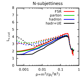
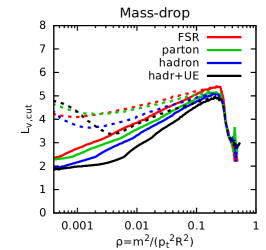
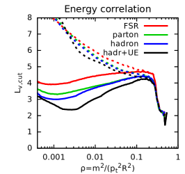
Finally, we want to investigate how the three shapes we have considered are affected by initial-state radiation (ISR) and non-perturbative effects such as hadronisation and the Underlying Event (UE). To get an insight about the importance of these effects, we have looked, for each jet mass, at the cut on $L_{v}$ that has to be applied to obtain a 25% tagging rate compared to the plain jet mass. This is plotted in Fig. 7 where we see that, as expected, the cuts are quite sensitive to ISR and the UE, with hadronisation effects remaining relatively small.

We attribute this behaviour to the sensitivity of the shapes to soft and large-angle radiation. We also see that the energy correlation function tends to be more sensitive to these effects than $N$-subjettiness and the mass-drop parameter.

These conclusions however have to be taken with a bit of care since the mass of the jet itself will also be subject to the non-perturbative effects. In practice, one would rarely use such a cut without some additional grooming of the jet, limiting the non-perturbative effects at least on the reconstruction of the jet mass. We will come back to this point later, in Section 6.

5 Calculations for the signal

We now turn to the case of signal jets, i.e. jets coming from boosted colourless objects that decay into a $q\bar{q}$ pair (or a pair of gluons), like a $W$, $Z$ or Higgs boson, or a photon.

As already briefly discussed in Sec. 3, the splitting of such a boosted object $X$ into a $q\bar{q}$ pair differs from a QCD gluon emission in the sense that it does not diverge as $1/z$ at small transverse-momentum fraction. This means that, although we are still in the regime $\rho\ll 1$ and we shall still consider the limit of small $v$ for all jet shapes $v$ we study in this paper, now $L_{1}=\log(1/z_{1})$ is no longer large. As for the case of QCD jets, we shall write the results as a function of $z_{1}$, see eq. (9), but now we will keep the correction in $z_{1}$ and $1-z_{1}$. These finite $z_{1}$ corrections would generate single-logarithmic terms under the form of contributions with one logarithm of $z_{1}$ or $1-z_{1}$ and one logarithm of $\rho$ or $v$. It is illustrative to expand out results in series of $\log(1/\rho)$ and $\log(1/v)$ to see explicitly how these terms appear. We shall do this in this Section and use a fixed-coupling approximation to better highlight the physics behind our calculation. In Appendices A.3 and A.4, we give the results with a running coupling. In that case, we found it easier to keep the $z_{1}$ dependence without making an explicit series expansion, knowing that both results are equivalent at single-logarithmic accuracy.

Besides the careful inclusion of the $z_{1}$ and $1-z_{1}$ dependence, the calculation follows the same logic as what has been done above and mostly consists of two copies of the contribution from “secondary emissions” in the QCD case, one for each of the decay products of the boosted colourless object. The contributions from each parton will just differ by the replacement $z_{1}\leftrightarrow(1-z_{1})$. For simplicity, we still use $L_{1}=\log(1/z_{1})$ and additionally introduce $L_{-}=\log(1/(1-z_{1}))$.

Finally, as was already seen to be the case for the secondary emission contributions for QCD jets, the results presented in this section apply invariantly for the recursive or non-recursive versions of the shapes.

5.1 $\tau_{21}$ cut

Following the same construction as in Section 4.1, we find that for an emission off the parton carrying a momentum $(1-z_{1})p_{t}$, we have

$$\tau_{21}=\frac{z_{2}\theta_{2}^{2}}{z_{1}\theta_{1}^{2}}.$$ (36)

This leads to

$$R_{\tau}(z_{1}) =\int_{0}^{\theta_{1}^{2}}\frac{d\theta_{2}^{2}}{\theta_{2}^{2}}\int_{0}^{1}dz_{2}\,\frac{\alpha_{s}(z_{2}\theta_{2})}{2\pi}\,P_{q}(z_{2})\,\Theta(z_{2}\theta_{2}^{2}/\theta_{1}^{2}>z_{1}\tau_{21})+[z_{1}\leftrightarrow(1-z_{1})],$$ (37)

where $\theta_{1}^{2}=\rho/[z_{1}(1-z_{1})]$.

For a fixed coupling approximation, and keeping only the first non-trivial terms in $L_{1}$ and $L_{-}$, terms we find

$$R_{\tau}^{{\rm(fixed)}}(z_{1})=\frac{\alpha_{s}C_{R}}{\pi}\left[L_{\tau}^{2}+(L_{1}+L_{-}+2B_{i})L_{\tau}\right].$$ (38)

5.2 $\mu^{2}$ cut

As for the case of QCD jets discussed in Section 4.2, expressions for $\mu^{2}$ differ from the $N$-subjettiness ones due to the fact that the $p_{t}$ normalisations are different.

For an emission off the parton carrying a momentum $(1-z_{1})p_{t}$, we have

$$\mu^{2}_{1/2}=\frac{(1-z_{1})z_{2}\theta_{2}^{2}}{z_{1}\theta_{1}^{2}}.$$ (39)

This leads to

$$R_{\mu^{2}_{1/2}}(z_{1}) =\int_{0}^{\theta_{1}^{2}}\frac{d\theta_{2}^{2}}{\theta_{2}^{2}}\int_{0}^{1}dz_{2}\,\frac{\alpha_{s}(z_{2}\theta_{2})}{2\pi}\,P_{q}(z_{2})\,\Theta(z_{2}\theta_{2}^{2}/\theta_{1}^{2}>z_{1}/(1-z_{1})\mu^{2}_{1/2})+[z_{1}\leftrightarrow(1-z_{1})]$$ (40)

Note that formally the $\Theta$ constraint above will result in the condition $\Theta(\mu^{2}<(1-z_{1})/z_{1})$ but this will only lead to power corrections in $\mu^{2}$ and can hence be neglected.

For a fixed coupling approximation the extra contributions from the two legs thus cancel, giving

$$R_{\mu^{2}_{1/2}}^{{\rm(fixed)}}(z_{1})=\frac{\alpha_{s}C_{R}}{\pi}\left[L_{\mu}^{2}+2B_{i}L_{\mu}\right].$$ (41)

Note that in the case of the signal, the calculation for $\mu_{0}^{2}$ would lead to the same result. However, other effects like soft and large-angle gluon emissions that we have neglected here would appear at the same order and lead to an infrared divergence for $\mu_{0}^{2}$.

5.3 $C_{2}$ cut

This time for emissions off the parton carrying a momentum $(1-z_{1})p_{t}$, we find

$$C_{2}=\frac{\rho}{z_{1}^{2}(1-z_{1})}\,z_{2}\,\frac{\theta_{2}^{2}}{\theta_{1}^{2}}.$$ (42)

This leads to

$$R_{C_{2}}(z_{1}) =\int_{0}^{\theta_{1}^{2}}\frac{d\theta_{2}^{2}}{\theta_{2}^{2}}\int_{0}^{1}dz_{2}\,\frac{\alpha_{s}(z_{2}\theta_{2})}{2\pi}\,P_{q}(z_{2})\,\Theta\Big{(}\frac{z_{2}\theta_{2}^{2}}{\theta_{1}^{2}}>\frac{z_{1}^{2}(1-z_{1})C_{2}}{\rho}\Big{)}+[z_{1}\leftrightarrow(1-z_{1})]$$ (43)

For a fixed coupling approximation, we get

$$R_{C_{2}}^{{\rm(fixed)}}(z_{1})=\frac{\alpha_{s}C_{R}}{\pi}\left[(L_{e}-L_{\rho})^{2}+(3L_{1}+3L_{-}+2B_{i})(L_{e}-L_{\rho})\right]\,\Theta(L_{e}>L_{\rho}).$$ (44)

Again, formally the extra factor $z_{1}^{2}(1-z_{1})$ will enter in the $\Theta(L_{e}>L_{\rho})$ condition but its effect is only power corrections and then can be neglected.

5.4 Integration over the $z_{1}$ splitting

For most of the splitting relevant for phenomenological studies, the splitting function in terms of $z_{1}$ is expressed as $z_{1}^{k}(1-z_{1})^{k}$ or as a linear combination of such terms (typically, only $k=0$ and $k=1$ are needed for $W/Z/H$ or photon signals).

Introducing $B_{2}(x)=B(x,x)=\Gamma^{2}(x)/\Gamma(2x)$, the integration over $z_{1}$ can be performed in the fixed-coupling approximation, using

$$\int_{0}^{1}dz_{1}\,z_{1}^{k}(1-z_{1})^{k}\exp\left(-\frac{\alpha_{s}C_{R}}{\pi}\,p\,L_{v}\,(L_{1}+L_{-})\right)=B_{2}\left(1+k+\frac{\alpha_{s}C_{R}}{\pi}\,pL_{v}\right),$$ (45)

with $p$ a number varying from one shape to another.

5.5 Comparison with fixed-order Monte-Carlo

Similarly to what was presented in Section 4.8 for QCD jets, we can compare our results with EVENT2 simulations. In this case, we boost the event along the $z$ axis and rotate it to obtain boosted photons decaying to a jet at $y=0$.

Figure 8: Distributions for the (non-recursive) shapes at order $\alpha_{s}$ for a few specific bins in the jet mass for the hadronic decay of a $Z$ boson. A constant factor $\alpha_{s}/(2\pi)$ has been factored out of the cross-section. The top row shows the distributions themselves, with solid lines corresponding to EVENT2 simulations and dashed lines to our analytic calculation. The bottom row shows the difference between the two.

The expansion of the above results to first order in $\alpha_{s}$ gives, after integration over $z_{1}$

$$\tau\frac{d\Sigma(\tau)}{d\tau} =\frac{\alpha_{s}C_{F}}{\pi}(2L_{\tau}+2B_{q}+a_{\gamma}),$$ (46)

$$\mu^{2}\,\frac{d\Sigma(\mu^{2})}{d\mu^{2}} =\frac{\alpha_{s}C_{F}}{\pi}(2L_{\mu}+2B_{q}),$$ (47)

$$C_{2}\,\frac{d\Sigma(C_{2})}{dC_{2}} =\frac{\alpha_{s}C_{F}}{\pi}\big{(}2(L_{e}-L_{\rho})+2B_{q}+3a_{\gamma}\big{)}\Theta(L_{e}>L_{\rho}).$$ (48)

In the above expressions, $a_{\gamma}=\frac{3}{2}a_{0}-\frac{1}{2}a_{1}=\frac{13}{6}$ with $a_{0}=2$ and $a_{1}=\frac{5}{3}$.

The comparison of these analytic results with EVENT2 simulations is presented in Fig. 8 and shows a good agreement. It is also interesting to notice that the convergence seems faster than it was for QCD jets, probably due to the fact that here the jet mass is fixed.

5.6 Comparison with parton-shower Monte-Carlo

Figure 9: Distributions obtained from $Z\to q\bar{q}$ jets for each of the three shapes studies. Left: results obtained with Pythia including only final-state radiation (for $4<L_{\rho}<4.5$); right: results of our analytic calculations (for $L_{\rho}=4.25$).

Figure 10: ROC curves showing the background fake rate as a function of the signal efficiency obtained from $Z\to q\bar{q}$ jets for each of the three shapes studies. Left: results obtained with Pythia including only final-state radiation (for $4<L_{\rho}<4.5$); right: results of our analytic calculations (for $L_{\rho}=4.25$).

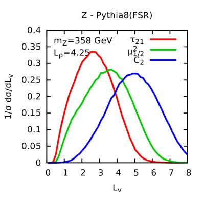
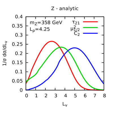
As for the case of the QCD background jets, we want to compare our analytic calculations to parton-shower Monte Carlo simulations. This time, we used Pythia to generate $ZZ$ events with both $Z$ bosons decaying to hadrons. To match the jet selection of Section 4.9 in the case of QCD jets, we have selected anti-$k_{t}$($R=1$) jets with $p_{t}\geq 3$ TeV and artificially varied the mass of the $Z$ boson to scan over the $\rho$ range.

The distributions obtained for the shapes are plotted on Fig. 9 for $Z$ bosons decaying hadronically. As for the case of QCD jets, we see a good overall description of the features of the distributions and of the differences between the three shapes, particularly in the large $L_{v}$ region which is targeted by our calculation.

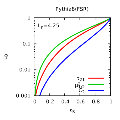
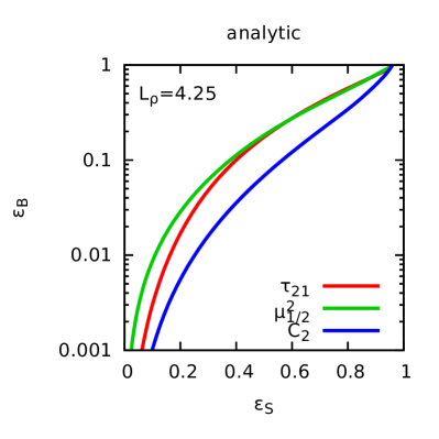
Based on the results for both the signal and the QCD background, we have plotted a set of ROC curves on Fig. 10 obtained by varying the cut on the three shapes for a given value of the jet mass. Note that here, the signal and background efficiencies are normalised to the sample of jets that are within the mass window under investigation. The main result here is that a cut on the energy correlation function is more efficient at rejecting the QCD background than a cut on $N$-subjettiness, itself performing a bit better than a cut on the mass-drop parameter. This behaviour is clearly seen in both the Pythia simulations and our analytic calculations. We leave a detailed discussion of this comparison for Section 7.

6 Non-perturbative effects and combination with grooming

Figure 11: Effects of the initial-state radiation (green), hadronisation (blue) and Underlying Event (black) on the ROC curves, compared to pure final-state radiation (red). In all cases, we impose that $5<\log(p_{t}^{2}R^{2}/m^{2})<5.5$. The left, central and right columns correspond to $\tau_{21}$, $\mu_{1/2}^{2}$ and $C_{2}$, respectively. For the top row, the mass and shape constraints are imposed on the plain, ungroomed, jet. For the plots on the bottom row, we have first applied a SoftDrop procedure with $\beta=2$ and $z_{\rm cut}=0.1$ before imposing the mass and shape constraints.

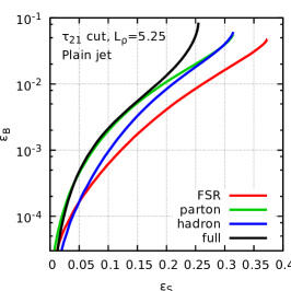
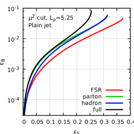
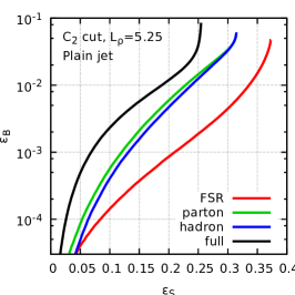
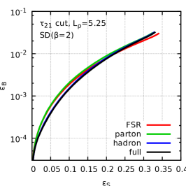
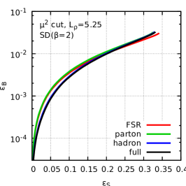
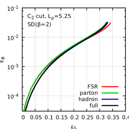
We have already seen in Section 4.9 and in Figure 7 that initial-state radiation and non-perturbative effects can have a large impact on the shapes we have studied. One difficulty in trying to assess these effects is that they do not only affect the different shapes we are interested in but also the jet mass and hence our selection of a sample of jets with a mass lying within a given window.

To make a physically meaningful comparison, we have to adapt our normalisation of the background and signal efficiencies compared to what we used to produce Figure 10. Instead, we shall now compute the efficiencies as the fraction of the jets passing the initial $p_{t}$ cut which satisfy both the constraint on the mass and the constraint on the shape. In such a case, as the cut on the shape increases, the signal and background efficiencies progressively increase to ultimately reach an endpoint, common to all shapes, where just the cut on the mass is effective.

As before, we work with anti-$k_{t}$ jets with $R=1$ and impose a $p_{t}$ cut of 3 TeV. For the signal, we used a massive $Z^{\prime}$ boson with a mass of 217 GeV and impose the constraint on the mass that $5<\log(p_{t}^{2}R^{2}/m^{2})<5.5$. Here the background is taken as quark-only to match with the results presented in the previous sections.

The top row of Fig. 11 show the ROC curves obtained for our three shapes starting from events including only final-state radiation effects at parton level (in red) and adding successively initial-state radiation (in green), hadronisation effects (in blue) and the Underlying Event (in black). We clearly see large deviations from what we observe for pure FSR results, noticeably when adding initial-state radiation and the Underlying Event. Concentrating on the endpoint of these curves, where the cut on the shapes has no effect, we see that these effects are already present when applying the initial mass cut.

In practice, when working with large-$R$ jets, one usually first applies a grooming procedure in order to obtain, at the very least, a good resolution on the jet mass. The bottom row of Fig. 11 shows the same plot as on the top row, now obtained by first grooming the jet with the SoftDrop procedure Larkoski:2014wba , using $z_{\rm cut}=0.1$ and $\beta=2$, before imposing the cut on the mass and on the shapes. Although this reduces the performance observed on events with pure final-state radiation, this has two positive effects: (i) it stabilises remarkably the ROC curves against initial-state radiation and non-perturbative effects, and (ii) at full parton level it even gives better performance than without the grooming procedure. Again, the ordering between the three shapes remains the same, albeit with strongly reduced differences compared to the plain jet case.

7 Discussion and conclusions

In this paper, we have provided a first-principles comparison of the performance of three common jet-shapes — $N$-subjettiness, the mass-drop parameter and Energy-Correlation Functions — used to discriminate boosted two-prong decays from QCD jets. In order to ensure infrared safety, we have defined the mass-drop parameter based on the subjets obtained via a clustering with the generalised $k_{t}$ algorithm with the extra parameter $p$ set to $1/2$. Similarly, for $N$-subjettiness, we find that using the exclusive gen-$k_{t}$($p=1/2$) algorithm is an efficient alternative to the more complicated optimal axes. The usage of the gen-$k_{t}$ algorithm is closely connected to the fact that it respects the ordering in mass, which is helpful in our situation where we work at a fixed jet mass and study shapes that have a mass-like behaviour.

The main observation from our analytical results and simulations involving only final-state radiation is that there appears to be a clear ordering in the discriminating power of the shapes we have studied: the energy-correlation function ratio is more powerful than the $N$-subjettiness ratio which, in turn, is more powerful than a cut on the $\mu^{2}$ parameter.

Our results indicate a Sudakov suppression of both the signal and the background for $v\ll 1$. This suppression is however more powerful for the background for two major reasons. Recall that, since we work at a fixed jet mass, both the QCD jets and the signal jets can be seen as two-pronged objects. A cut on the shape thus constrains additional radiation from that system. Given that, discrimination power comes from constraints on radiation at angles smaller and larger than the opening angle between the two prongs. For large angles, the cut on the shape only affects the background due to the colour-singlet nature of the signal. At small angles, the radiation from each of the two prongs is proportional to their colour factors, which tend to be larger for QCD jets, involving gluons in their two-prong decay, than for resonances mostly decaying to quarks. Since we know from experience with quark-gluon discrimination that exploiting differences in colour factors only lead to moderate discrimination power Larkoski:2013eya ; Gallicchio:2011xq ; Larkoski:2014pca ; Aad:2014gea , we expect that the large-angle effect would be the main source of difference in tagging two-body decays.

The ordering in discrimination power between the different shapes can also be understood from that viewpoint. Say we work at a given signal efficiency. The corresponding cut on the shape would determine the constraints on small-angle radiation for both the signal and the background (up to colour-factor effects discussed above). Once this is fixed, one has to look at the constraint put on the large-angle radiation for QCD jets. In that region, it is clear from our results, that the radiation veto imposed by a cut on $C_{2}$ is more constraining than that imposed by a cut on $\tau_{21}$, itself more constraining than a cut on $\mu^{2}$. This can be deduced from Fig. 1: fixing the signal efficiency amounts to fix the rejected region at small angle and once this is held equal for all three shapes, the vetoed region at large angle shows a clear ordering between $C_{2}$, $\tau_{21}$ and $\mu^{2}$.

Figure 12: Background fake rate for a 25% signal efficiency as a function of the jet mass. As above, we used $R=1$ and $p_{t,\rm jet}>3$ TeV for the Pythia simulation (left plot) and $p_{t}=3$ TeV, for the analytic calculation (right plot).

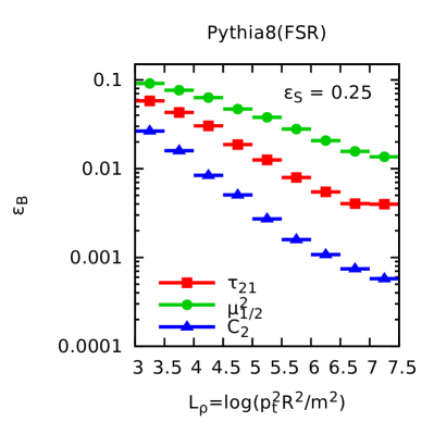
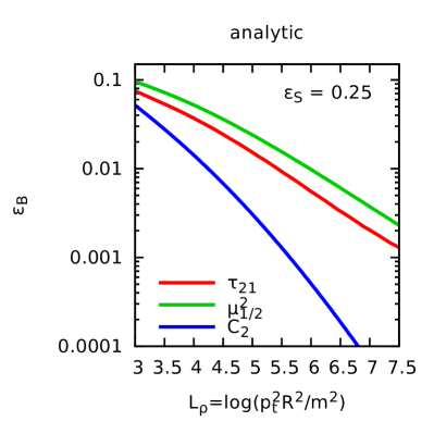
This statement can be made more quantitative from our analytic results. First, the difference between $\tau_{21}$ and $\mu^{2}$ mostly comes from the large-angle region where gluon emissions are clustered with the gluon setting the mass. The extra $z_{1}$ factor in the expression for $\mu^{2}$ compared to $\tau_{21}$, see Eq. (11) v. (15), results in a smaller vetoed region for $\mu^{2}$. Parametrically, this region scales like $\alpha_{s}\log(1/\theta_{1}^{2})\log(1/v)\propto\alpha_{s}\log(1/\rho)\log(1/v)$. This can be deduced algebraically from our results by fixing the signal efficiency and computing the background for the corresponding cut (with additional $\alpha_{s}\log^{2}(1/v)$ terms also coming from the small-angle region). In the case of $C_{2}$, the constraint at large angle now becomes proportional to $\theta_{2}^{4}$, see Eq. (18), and this translates into an additional vetoed region compared to $\tau_{21}$ which is proportional to $\alpha_{s}\log^{2}(1/\theta_{1}^{2})\propto\alpha_{s}\log^{2}(1/\rho)$. In conclusion, we expect the ordering between the shapes to be more visible when increasing the boost of the jet. This difference should also grow faster with $p_{t}/m$ when comparing $C_{2}$ and $\tau_{21}$ than for $\tau_{21}$ and $\mu^{2}$. This is indeed what is observed from both pure-FSR Monte-Carlo studies and from our analytic calculations, as seen in Fig. 12, where we have plotted the background rejection rate for a 25% signal efficiency as a function of $\log(1/\rho)=\log(p_{t}^{2}R^{2}/m^{2})$.

Note that our explanation of the differences between $C_{2}$ and $\tau_{21}$ is consistent with a similar observation made in Larkoski:2013eya but our more detailed analytic treatment allows for more quantitative understanding.

The next important observation is that, without grooming, the shapes are significantly affected by ISR and non-perturbative effects, UE in particular. These model-dependent effects can be substantial enough to wash out or even invert the differences between the shapes observed from pure FSR and analytic studies (see e.g. the top row of Fig. 11). This is due to the impact of these effects on both the mass resolution for the jet — mostly for signal jets — and the sensitivity of the shapes themselves. Since ISR and UE mostly affect the soft-and-large-angle region, we expect $C_{2}$ to be more affected than $\tau_{21}$, itself more affected than $\mu^{2}$ (see the discussion above) and this is indeed what we observe from Monte Carlo studies.

Furthermore, we have seen that applying a grooming procedure on the jet before computing its mass and values of the shapes largely improves the robustness against ISR and non-perturbative effects, also restoring the ordering between the shapes observed with pure FSR. Again, this can be interpreted as grooming cutting away a part of the soft-and-large-angle region. This increased robustness however comes at a price in that reducing the soft-and-large-angle region using grooming also reduces the discriminating power of the shape cuts. In practice, there will be a trade-off between sheer efficiency and robustness against model-dependent effects. We reserve the detailed study of an optimal combination of a shape cut with a proper grooming procedure for future work.

In addition, note that working at a fixed jet mass ensures that our results are infrared-and collinear safe because it fixes automatically the value of $\tau_{1}$ and $e_{2}$. If we were to impose a cut on the shapes without fixing the jet mass, our results would still be finite after integration of (3) over $\rho$ because the infrared region is killed by the plain mass Sudakov. This is an example of Sudakov-safe observables Larkoski:2013paa ; Larkoski:2015lea . It is interesting to note that, after integration over the jet mass, we recover a distribution that can be expressed as a series in $\sqrt{\alpha_{s}}\log(1/v)$, similar to what was obtained for ratios of angularities in Larkoski:2013paa .

The arguments above can be applied when comparing the recursive and non-recursive versions of the shapes: the recursive versions have a smaller vetoed region at large angle while retaining the same small-angle region as their corresponding non-recursive version. Thus, although the recursive versions have the advantage of being less sensitive to ISR and non-perturbative effects, they have a smaller discriminating power. A combination of a non-recursive cut on the shape with a proper grooming of the jet is expected to perform better while at the same time limiting non-perturbative effects.

Another key aspect of our results is that a cut on the shapes leads to an exponential suppression of the signal efficiency. This has to be contrasted with two-prong taggers like the mass-drop tagger, trimming or pruning which would only give a linear suppression Dasgupta:2015yua . This means that although it initially seems natural to work in the small $v$ limit, in practice one will not be able to take the cut on $v$ too small. Computing corrections for finite $v$ could then become relevant for this discussion.

Finally, there are several other developments that can be made based on this study. In this paper, we have focused on a subset of jet shapes sensitive to the mass of the subjets. It would be interesting to extend this study to more generic jet shapes, e.g. studying the $\beta$ dependence of energy-correlation-function ratios and $N$-subjettiness ratios. On the more formal side, we could also refine our calculations to include effects such as the initial-state radiation and finite jet radius contributions as well as attaining full NLL accuracy, optionally matched to a fixed-order calculation.

Appendix A Results with running coupling: QCD background

Results including running-coupling corrections can be straightforwardly obtained from the expressions before integration over $z_{2}$ and $\theta_{2}$ given in Section 4. The running of the coupling is expressed wrt its value $\alpha_{s}\equiv\alpha_{s}(p_{t}R)$ taken at the physical scale of the problem, $p_{t}R$, using the CMW scheme as appropriate for resummations Catani:1990rr ; Dokshitzer:1995ev . We also freeze the coupling at a scale $\mu_{\rm fr}$, giving

$$\alpha_{s}(k_{t})=\frac{\alpha_{s}}{D}-\alpha_{s}^{2}\frac{\beta_{1}}{\beta_{0}}\frac{\log(D)}{D^{2}}+\alpha_{s}^{2}\frac{K}{2\pi}\frac{1}{D^{2}},\text{ with }D=1+2\alpha_{s}\beta_{0}\log\left(\frac{\max(k_{t},\mu_{\rm fr})}{p_{t}R}\right)$$ (49)

with

$$\beta_{0}=\frac{11C_{A}-2n_{f}}{12\pi},\quad\beta_{1}=\frac{17C_{A}^{2}-5C_{A}n_{f}-3C_{F}n_{f}}{24\pi^{2}},\quad K=\left(\frac{67}{18}-\frac{\pi^{2}}{6}\right)C_{A}-\frac{5}{9}n_{f}.$$ (50)

To keep the notations concise, we introduce $\lambda_{x}=2\alpha_{s}\beta_{0}L_{x}$ where $L_{x}$ denotes any symbol we have introduced in (10) and $L_{\rm fr}=\log(p_{t}R/\mu_{\rm fr})=\log(1/\tilde{\mu}_{\rm fr})$.

A.1 Basic building blocks

     

Figure 13: Left: representation of the basic building block used to present our results. It appears in two different forms whether we have $\alpha<1$ or $\alpha>1$. Right: two additional fundamental objects built from $T_{\alpha}$.

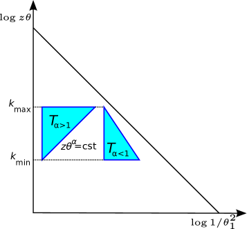
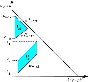
It is helpful to introduce a few building blocks that will greatly help in writing the several results below in a short and understandable way.

The most basic building block we shall use is the integral over a “triangle” bounded by a maximal angle, a constant $k_{t}\propto z\theta$ line (upper or lower bound) and a constant generic line of constant $z\theta^{\alpha}$, as represented on Fig. 13. Expressed as a function of the minimal and maximal $k_{t}$ scales of this triangle, this triangle can be written as

$$T_{\alpha}(k_{\max},k_{\min};C_{R},B_{i})$$

$$\quad\overset{\alpha<1}{=}\int\frac{d\theta^{2}}{\theta^{2}}\,dz\,P(z)\,\frac{\alpha(z\theta)}{2\pi}\,\Theta(\theta<k_{\max})\,\Theta(z\theta>k_{\min})\,\theta(z\theta^{\alpha}<k_{\max}^{\alpha})$$ (51)

$$\quad\overset{\alpha>1}{=}\int\frac{d\theta^{2}}{\theta^{2}}\,dz\,P(z)\,\frac{\alpha(z\theta)}{2\pi}\,\Theta(\theta<1)\,\Theta(z\theta<k_{\max})\,\theta(z\theta^{\alpha}>k_{\min})$$ (52)

The exact expressions for these integrals depend on the positions of $k_{\min}$ and $k_{\max}$ compared to $\tilde{\mu}_{\rm fr}$. For $k_{\min}>\tilde{\mu}_{\rm fr}$ we find, introducing $L_{\min}=\log(1/k_{\min})$, $\lambda_{\min}=2\alpha_{s}\beta_{0}L_{\min}$ and similar quantities associated with $k_{\max}$,

$$T_{\alpha}(k_{\max},k_{\min};C_{R},B_{i})$$ (53)

$$\;\;\overset{\alpha<1}{=}\frac{C_{R}}{2\pi\alpha_{s}\beta_{0}^{2}}\frac{1}{1-\alpha}\Big{\{}\Big{[}(1\!-\!\lambda_{\max}+2\alpha_{s}\beta_{0}B_{i}\Theta(\alpha=0))\log\Big{(}\frac{1\!-\!\lambda_{\max}}{1\!-\!\lambda_{\min}}\Big{)}+\lambda_{\max}-\lambda_{\min}\Big{]}$$

$$\qquad-\frac{\alpha_{s}\beta_{1}}{\beta_{0}}\Big{[}\frac{1}{2}\log^{2}(1\!-\!\lambda_{\min})-\frac{1}{2}\log^{2}(1\!-\!\lambda_{\max})+\frac{1\!-\!\lambda_{\max}}{1\!-\!\lambda_{\min}}\log(1\!-\!\lambda_{\min})-\log(1\!-\!\lambda_{\max})$$

$$\phantom{\qquad-\frac{\alpha_{s}\beta_{1}}{\beta_{0}}\;}+\frac{\lambda_{\min}-\lambda_{\max}}{1\!-\!\lambda_{\min}}\Big{]}+\frac{\alpha_{s}K}{2\pi}\Big{[}\log\Big{(}\frac{1\!-\!\lambda_{\min}}{1\!-\!\lambda_{\max}}\Big{)}+\frac{\lambda_{\min}-\lambda_{\max}}{1\!-\!\lambda_{\min}}\Big{]}\Big{\}}$$

$$\;\;\overset{\alpha>1}{=}\frac{C_{R}}{2\pi\alpha_{s}\beta_{0}^{2}}\frac{1}{\alpha-1}\Big{\{}\Big{[}(1\!-\!\lambda_{\min})\log\Big{(}\frac{1\!-\!\lambda_{\min}}{1\!-\!\lambda_{\max}}\Big{)}+\lambda_{\min}-\lambda_{\max}\Big{]}$$

$$\qquad-\frac{\alpha_{s}\beta_{1}}{\beta_{0}}\Big{[}\frac{1}{2}\log^{2}(1\!-\!\lambda_{\max})-\frac{1}{2}\log^{2}(1\!-\!\lambda_{\min})+\frac{1\!-\!\lambda_{\min}}{1\!-\!\lambda_{\max}}\log(1\!-\!\lambda_{\max})-\log(1\!-\!\lambda_{\min})$$

$$\phantom{\qquad-\frac{\alpha_{s}\beta_{1}}{\beta_{0}}\;}+\frac{\lambda_{\max}-\lambda_{\min}}{1\!-\!\lambda_{\max}}\Big{]}+\frac{\alpha_{s}K}{2\pi}\Big{[}\log\Big{(}\frac{1\!-\!\lambda_{\max}}{1\!-\!\lambda_{\min}}\Big{)}+\frac{\lambda_{\max}-\lambda_{\min}}{1\!-\!\lambda_{\max}}\Big{]}\Big{\}},$$

where the $B_{i}$ term for $\alpha<1$ only has to be included if the “triangle” upper edge corresponds to $z=1$. For $k_{\min}<\tilde{\mu}_{\rm fr}$ but $k_{\max}>\tilde{\mu}_{\rm fr}$, one obtains

$$T_{\alpha}(k_{\max},k_{\min};C_{R},B_{i})$$ (54)

$$\;\;\overset{\alpha<1}{=}\frac{C_{R}}{2\pi\alpha_{s}\beta_{0}^{2}}\frac{1}{1-\alpha}\Big{\{}\Big{[}(1\!-\!\lambda_{\max}+2\alpha_{s}\beta_{0}B_{i}\Theta(\alpha=0))\log\Big{(}\frac{1\!-\!\lambda_{\max}}{1\!-\!\lambda_{\rm fr}}\Big{)}+\lambda_{\max}-\lambda_{\rm fr}\Big{]}$$

$$\qquad-\frac{\alpha_{s}\beta_{1}}{\beta_{0}}\Big{[}\frac{1}{2}\log^{2}(1\!-\!\lambda_{\rm fr})-\frac{1}{2}\log^{2}(1\!-\!\lambda_{\max})+\frac{1\!-\!\lambda_{\max}}{1\!-\!\lambda_{\rm fr}}\log(1\!-\!\lambda_{\rm fr})-\log(1\!-\!\lambda_{\max})$$

$$\phantom{\qquad-\frac{\alpha_{s}\beta_{1}}{\beta_{0}}\;}+\frac{\lambda_{\rm fr}-\lambda_{\max}}{1\!-\!\lambda_{\rm fr}}\Big{]}+\frac{\alpha_{s}K}{2\pi}\Big{[}\log\Big{(}\frac{1\!-\!\lambda_{\rm fr}}{1\!-\!\lambda_{\max}}\Big{)}+\frac{\lambda_{\rm fr}-\lambda_{\max}}{1\!-\!\lambda_{\rm fr}}\Big{]}\Big{\}}$$

$$\qquad+\frac{C_{R}}{\pi(1-\alpha)}(L_{\min}-L_{\rm fr})\big{[}\alpha_{s}(\tilde{\mu}_{\rm fr})(L_{\min}+L_{\rm fr}-2L_{\max})+2\alpha_{s,\text{1-loop}}(\tilde{\mu}_{\rm fr})B_{i}\Theta(\alpha=0)\big{]}$$

$$\;\;\overset{\alpha>1}{=}\frac{C_{R}}{2\pi\alpha_{s}\beta_{0}^{2}}\frac{1}{\alpha-1}\Big{\{}\Big{[}(1\!-\!\lambda_{\min})\log\Big{(}\frac{1\!-\!\lambda_{\rm fr}}{1\!-\!\lambda_{\max}}\Big{)}+\lambda_{\rm fr}-\lambda_{\max}\Big{]}$$

$$\qquad-\frac{\alpha_{s}\beta_{1}}{\beta_{0}}\Big{[}\frac{1}{2}\log^{2}(1\!-\!\lambda_{\max})-\frac{1}{2}\log^{2}(1\!-\!\lambda_{\rm fr})+\frac{1\!-\!\lambda_{\min}}{1\!-\!\lambda_{\max}}\log(1\!-\!\lambda_{\max})-\frac{1\!-\!\lambda_{\min}}{1\!-\!\lambda_{\rm fr}}\log(1\!-\!\lambda_{\rm fr})$$

$$\phantom{\qquad-\frac{\alpha_{s}\beta_{1}}{\beta_{0}}\;}+\frac{(\lambda_{\max}\!-\!\lambda_{\rm fr})(1\!-\!\lambda_{\min})}{(1\!-\!\lambda_{\max})(1\!-\!\lambda_{\rm fr})}\Big{]}+\frac{\alpha_{s}K}{2\pi}\Big{[}\log\Big{(}\frac{1\!-\!\lambda_{\max}}{1\!-\!\lambda_{\rm fr}}\Big{)}+\frac{(\lambda_{\max}\!-\!\lambda_{\rm fr})(1\!-\!\lambda_{\min})}{(1\!-\!\lambda_{\max})(1\!-\!\lambda_{\rm fr})}\Big{]}\Big{\}},$$

$$\qquad+\frac{\alpha_{s}(\tilde{\mu}_{\rm fr})C_{R}}{\pi(\alpha-1)}(L_{\min}-L_{\rm fr})^{2}.$$

In that expression, we have introduced $\alpha_{s,\text{1-loop}}(k_{t})=\alpha_{s}/(1-2\alpha_{s}\beta_{0}\log(p_{t}R/k_{t}))$, the running-coupling at 1-loop, which multiplies the contributions proportional to $B_{i}$ in the frozen region. This reflects the fact that contributions proportional to $\beta_{1}B_{i}$ and $KB_{i}$, coming from the 2-loop corrections to the running of $\alpha_{s}$ are subleading. They are not included, neither in the frozen region, nor in the running-coupling region.

And, finally, for $k_{\max}<\tilde{\mu}_{\rm fr}$, one gets

$$T_{\alpha}(k_{\max},k_{\min};C_{R},B_{i})$$ (55)

$$\quad=\frac{C_{R}}{\pi|1-\alpha|}(L_{\min}-L_{\max})\big{[}\alpha_{s}(\tilde{\mu}_{\rm fr})(L_{\min}-L_{\max})+2\alpha_{s,\text{1-loop}}(\tilde{\mu}_{\rm fr})B_{i}\Theta(\alpha=0)\big{]}.$$

From this fundamental building block, we can build two derived objects which will be used to describe all the expressions we have below. The first one is again a triangle bound by a maximal angle, a maximal $z\theta^{\alpha}$ line and a minimal $z\theta^{\beta}$ line, see the right plot of Fig. 13. This can be seen as a superposition of two of the above triangles. Again, we can express this new object as a function of the minimal and maximal $k_{t}$ scales on the maximal-angle side of the triangle, and, assuming $\alpha<\beta$, we get

$$T_{\alpha\beta}(k_{\max},k_{\min};C_{R},B_{i}) \overset{\alpha<\beta<1}{=}T_{\alpha}(k_{\max},k_{\rm med};C_{R},B_{i})-T_{\beta}(k_{\min},k_{\rm med};C_{R},B_{i})$$ (56)

$$\overset{\alpha<1<\beta}{=}T_{\alpha}(k_{\max},k_{\rm med};C_{R},B_{i})+T_{\beta}(k_{\rm med},k_{\min};C_{R},B_{i})$$ (57)

$$\overset{1<\alpha<\beta}{=}T_{\beta}(k_{\rm med},k_{\min};C_{R},B_{i})-T_{\alpha}(k_{\rm med},k_{\max};C_{R},B_{i}),$$ (58)

with $k_{\rm med}=k_{\max}^{\frac{\beta-1}{\beta-\alpha}}k_{\min}^{\frac{1-\alpha}{\beta-\alpha}}$.

The last object we shall use is a “parallelogram” bounded by a minimal and a maximal angle and two parallel lines of constant $z\theta^{\alpha}$, assuming here $\alpha>1$, see again the right plot of Fig. 13. This is expressed as a function of the maximal $k_{t}$ scale $k_{1}$ (at the minimal angle) and the maximal and minimal $k_{t}$ scales, $k_{2}$ and $k_{3}$ at the maximal angle. We can view this as a function of three of our basic triangles

$$P_{\alpha}(k_{1},k_{2},k_{3};C_{R})=T_{\alpha}(k_{1},k_{3};C_{R},0)-T_{\alpha}(k_{1},k_{2};C_{R},0)-T_{\alpha}(k_{1},k_{4};C_{R},0)$$ (59)

with $k_{4}=k_{1}k_{3}/k_{2}$.

Note that we will often substitute the $k_{t}$ scale with their logarithm, $\log(1/k_{t})$ and it is worth keeping in mind that the maximal $k_{t}$ would correspond to the minimal $\log(1/k_{t})$.

A.2 Results for the QCD background

Now that we have building blocks corresponding to the integration of Sudakov factors over basic phase-space regions, we can use them to find simple expressions for the Sudakov factors corresponding to the shapes we are studying.

The phase-space regions will correspond exactly to the regions we have already used for the fixed-coupling calculation given in the main text, so we just list the results here.

$N$-subjettiness.

This is the most simple result because the phase-space just corresponds to a triangle for the primary emissions and another one for the secondary emissions:

$$R_{\tau}(z_{1}) =T_{02}(0,L_{\rho}+L_{v};C_{R},B_{i})-T_{02}(0,L_{\rho};C_{R},B_{i})$$

$$+T_{02}\Big{(}\frac{L_{\rho}+L_{1}}{2},\frac{L_{\rho}+L_{1}}{2}+L_{v};C_{A},B_{g}\Big{)},$$ (60)

where the negative term subtracts the Sudakov factor for the plain jet mass which has been factored out in our expressions.

Mass-drop (non-recursive).

Here we split the result in a part, $R_{0}$ clustered with the main parton and a part, $R_{1}$, clustered with the emission setting the mass.

$$R_{\mu_{1/2}^{2},0}(z_{1}) =T_{02}\Big{(}\frac{L_{\rho}-L_{1}}{2},\frac{L_{\rho}+L_{1}}{2}+L_{v};C_{R},B_{i}\Big{)}-T_{02}\Big{(}\frac{L_{\rho}-L_{1}}{2},\frac{L_{\rho}+L_{1}}{2};C_{R},B_{i}\Big{)}$$

$$+\frac{1}{2}P_{2}\Big{(}\frac{L_{\rho}+L_{1}}{2},L_{\rho},L_{\rho}+L_{v};C_{R},B_{i}\Big{)}$$

$$R_{\mu_{1/2}^{2},1}(z_{1}) =\Big{[}\frac{1}{2}P_{2}\Big{(}\frac{L_{\rho}+L_{1}}{2},L_{\rho},L_{\rho}-L_{1}+L_{v};C_{R},B_{i}\Big{)}$$

$$\phantom{=\Big{[}}+T_{02}\Big{(}\frac{L_{\rho}+L_{1}}{2},\frac{L_{\rho}-L_{1}}{2}+L_{v};C_{A},B_{g}\Big{)}\Big{]}\,\Theta(L_{v}>L_{1})$$ (61)

The total Sudakov $R_{\mu_{1/2}^{2}}$ is the sum of these two contributions.

Energy correlation function.

For $C_{2}$ we have to disentangle two cases depending on whether we have a contribution from emissions at small angles of not:

$$R_{C_{2}}(z_{1}) \overset{L_{v}<L_{\rho}-L_{1}}{=}T_{24}(L_{\rho},L_{\rho}+L_{v};C_{R},B_{i})$$

$$\overset{L_{v}>L_{\rho}-L_{1}}{=}T_{02}(0,L_{\rho}-L_{1}+L_{v};C_{R},B_{i})-T_{02}(0,L_{\rho};C_{R},B_{i})$$ (62)

$$\phantom{\overset{L_{v}>L_{\rho}-L}{=}}+T_{24}(L_{1}+L_{v},L_{\rho}+L_{v};C_{R},B_{i})+T_{02}\Big{(}\frac{L_{\rho}+L_{1}}{2},\frac{3L_{1}-L_{\rho}}{2}+L_{v};C_{A},B_{g}\Big{)}$$

This expression can be trivially expressed as a result for $D_{2}$ replacing $L_{v}$ by $L_{v}-L_{\rho}$.

Recursive $N$-subjettiness.

Here, the phase-space constraints can take three different forms. Remember also that we do subtract the Sudakov factor corresponding to the plain jet mass.

$$R_{\tau,\rm rec}(z_{1}) \overset{L_{v}<L_{1}}{\quad\;\;=\quad\;\;}T_{02}\Big{(}\frac{L_{\rho}-L_{1}}{2},\frac{L_{\rho}+L_{1}}{2}+L_{v};C_{R},B_{i}\Big{)}-T_{02}\Big{(}\frac{L_{\rho}-L_{1}}{2},\frac{L_{\rho}+L_{1}}{2};C_{R},B_{i}\Big{)}$$

$$\phantom{\overset{L_{v}>L}{\quad\;\;=\quad\;\;}}-P_{2}\Big{(}\frac{L_{\rho}-L_{1}}{2}-L_{v},L_{\rho}-L_{v},L_{\rho};C_{R},B_{i}\Big{)}$$

$$\phantom{\overset{L_{v}>L}{\quad\;\;=\quad\;\;}}+T_{02}\Big{(}\frac{L_{\rho}+L_{1}}{2},\frac{L_{\rho}+L_{1}}{2}+L_{v};C_{A},B_{g}\Big{)}$$

$$\overset{L_{1}<L_{v}<L_{\rho}}{\quad\;\;=\quad\;\;}T_{02}\Big{(}\frac{L_{\rho}-L_{1}}{2},\frac{L_{\rho}+L_{1}}{2}+L_{v};C_{R},B_{i}\Big{)}+T_{02}(0,L_{v}-L_{\rho};C_{R},B_{i})$$

$$\phantom{\overset{L_{v}>L}{\quad\;\;=\quad\;\;}}-T_{02}(0,L_{\rho};C_{R},B_{i})+T_{02}\Big{(}\frac{L_{\rho}+L_{1}}{2},\frac{L_{\rho}+L_{1}}{2}+L_{v};C_{A},B_{g}\Big{)}$$

$$\overset{L_{v}>L_{\rho}}{\quad\;\;=\quad\;\;}T_{02}\Big{(}\frac{L_{\rho}-L_{1}}{2},\frac{L_{\rho}+L_{1}}{2}+L_{v};C_{R},B_{i}\Big{)}-T_{02}(0,L_{\rho};C_{R},B_{i})$$

$$\phantom{\overset{L_{v}>L}{\quad\;\;=\quad\;\;}}+T_{02}\Big{(}\frac{L_{\rho}+L_{1}}{2},\frac{L_{\rho}+L_{1}}{2}+L_{v};C_{A},B_{g}\Big{)}$$ (63)

Recursive Mass-drop.

The expression is the same as for the recursive $N$-subjettiness cut,Eq. (63), except that the second argument of the $C_{A}$ term should be $\frac{L_{\rho}-L_{1}}{2}+L_{v}$ instead of $\frac{L_{\rho}+L_{1}}{2}+L_{v}$ and that term comes with a $\Theta(L_{v}>L_{1})$.

Recursive energy correlation function.

Again, we have three different situations

$$R_{C_{2},\rm rec}(z_{1}) \overset{L_{v}<L_{\rho}-L_{1}}{\quad\;\;=\quad\;\;}-T_{02}(L_{\rho}-L_{v},L_{\rho};C_{R},B_{i}\Big{)}$$

$$\overset{L_{v}<L_{\rho}}{\quad\;\;=\quad\;\;}T_{02}\Big{(}\frac{L_{\rho}-L_{1}}{2},\frac{3L_{1}-L_{\rho}}{2}+L_{v};C_{R},B_{i}\Big{)}-T_{02}\Big{(}\frac{L_{\rho}-L_{1}}{2},\frac{L_{\rho}+L_{1}}{2};C_{R},B_{i}\Big{)}$$

$$\phantom{\overset{L_{v}>L}{\quad\;\;=\quad\;\;}}-T_{02}(L_{\rho}-L_{v},L_{\rho};C_{R},B_{i})+T_{02}\Big{(}\frac{3L_{\rho}-L_{1}}{2}-L_{v},\frac{L_{\rho}+L_{1}}{2};C_{R},B_{i}\Big{)}$$

$$\phantom{\overset{L_{v}>L}{\quad\;\;=\quad\;\;}}+T_{02}\Big{(}\frac{L_{\rho}+L_{1}}{2},\frac{3L_{1}-L_{\rho}}{2}+L_{v};C_{A},B_{g}\Big{)}$$

$$\overset{L_{v}>L_{\rho}}{\quad\;\;=\quad\;\;}T_{02}\Big{(}\frac{L_{\rho}-L_{1}}{2},\frac{3L_{1}-L_{\rho}}{2}+L_{v};C_{R},B_{i}\Big{)}-T_{02}(0,L_{\rho};C_{R},B_{i})$$

$$\phantom{\overset{L_{v}>L}{\quad\;\;=\quad\;\;}}+T_{02}\Big{(}\frac{L_{\rho}+L_{1}}{2},\frac{3L_{1}-L_{\rho}}{2}+L_{v};C_{A},B_{g}\Big{)}$$ (64)

This expression can be trivially expressed as a result for $D_{2}$ replacing $L_{v}$ by $L_{v}-L_{\rho}$.

A.3 Results for the signal

As previously, it is fairly straightforward to use the “triangular” building blocks to express our findings. Note also that, compared to the results presented for fixed-coupling in the main text, we have not expanded our results to first order in $z_{1}$ and $1-z_{1}$. This would only lead to more complicated expressions without changing the formal accuracy of our results. Remember also that for the case of signal jets and at NLL (and small-$R$) accuracy, the results are the same for the recursive and non-recursive versions of the shapes.

$N$-subjettiness (recursive or non-recursive).

From the expression in eq. (37) it is easy to find

$$R_{\tau}(z_{1}) =T_{02}\Big{(}\frac{L_{\rho}+L_{-}-L_{1}}{2},\frac{L_{\rho}+L_{-}+L_{1}}{2}+L_{v};C_{R},B_{i}\Big{)}$$ (65)

$$+T_{02}\Big{(}\frac{L_{\rho}+L_{1}-L_{-}}{2},\frac{L_{\rho}+L_{1}+L_{-}}{2}+L_{v};C_{R},B_{i}\Big{)}$$

Mass-drop (recursive or non-recursive).

As for the fixed-coupling case, the only difference between $N$-subjettiness and a $\mu_{1/2}^{2}$ cut lies in the $z_{1}$ and $1-z_{1}$ corrections. We find

$$R_{\mu_{1/2}^{2}}(z_{1}) =T_{02}\Big{(}\frac{L_{\rho}+L_{-}-L_{1}}{2},\frac{L_{\rho}-L_{-}+L_{1}}{2}+L_{v};C_{R},B_{i}\Big{)}\,\Theta(L_{v}>L_{-}-L_{1})$$ (66)

$$+T_{02}\Big{(}\frac{L_{\rho}+L_{1}-L_{-}}{2},\frac{L_{\rho}-L_{1}+L_{-}}{2}+L_{v};C_{R},B_{i}\Big{)}\,\Theta(L_{v}>L_{1}-L_{-})$$

Energy correlation function (recursive or non-recursive).

Again, the expression for $C_{2}$ looks very similar, except for the logarithms involving $z_{1}$. We find

$$R_{C_{2}}(z_{1}) =T_{02}\Big{(}\frac{L_{\rho}+L_{-}-L_{1}}{2},\frac{3L_{-}+3L_{1}-L_{\rho}}{2}+L_{v};C_{R},B_{i}\Big{)}\,\Theta(L_{v}>L_{\rho}-L_{-}-2L_{1})$$ (67)

$$+T_{02}\Big{(}\frac{L_{\rho}+L_{1}-L_{-}}{2},\frac{3L_{1}+3L_{-}-L_{\rho}}{2}+L_{v};C_{R},B_{i}\Big{)}\,\Theta(L_{v}>L_{\rho}-L_{1}-2L_{-})$$

This expression can be trivially expressed as a result for $D_{2}$ replacing $L_{v}$ by $L_{v}-L_{\rho}$.

A.4 Including finite $z_{1}$ corrections: QCD (background) and signal jets

We have argued in Section 4.7 that if we wish to achieve NLL accuracy it is mandatory to include all finite $z_{1}$ and $1-z_{1}$ factors in our expressions for the shapes, with $z_{1}$ the fraction of the jet transverse momentum carried by the emission that dominates the mass of the jet. The main reason behind that is that they can be raised to powers of order $\alpha_{s}\log(1/v)$ which would give single-logarithmic corrections after integration over $z_{1}$.

Figure 14: Three topologies potentially contributing to the emission of the gluon dominating the value of the shape, starting with a massive two-pronged object. Left: small-angle emission from the prong carrying a fraction $1-z_{1}$ of the jet $p_{t}$ (“prong 1”), centre: small-angle emission from the prong carrying a fraction $z_{1}$ of the jet $p_{t}$ (“prong 2”), right: large-angle emission from the parent object (“parent”).

In this Section, our main goal is to discuss these extra source of NLL terms. As a fringe benefit of this discussion, we will at the same time provide a unified description of the signal and background distributions, allowing for interesting interpretations of the results obtained in this paper.

If we want to properly include the finite $z_{1}$ corrections we first need to carefully identify the origin of the gluon emissions. In the collinear limit, sufficient to capture all the finite $z_{1}$ corrections, colour coherence indicates that we can encounter three situations, represented in Fig. 14. The first two situations correspond to gluon emissions at small angle $\theta_{2}\ll\theta_{1}$ from the splitting of either the hardest or the softest of the two prongs (carrying respectively a fraction $1-z_{1}$ and $z_{1}$ of the jet transverse momentum). These are the first two plots of Fig. 14 and will be referred to as the “prong 1” and “prong 2” topologies respectively for the $1-z_{1}$ and $z_{1}$ case. The third option corresponds to gluons emitted at large angle $\theta_{2}\gg\theta_{1}$ from the parent parton in the jet. This is represented on the rightmost plot of Fig. 14 and will be called the “parent” topology in what follows. In that approach, the distribution for QCD jets will receive contributions from all three topologies — the first and third weighted by $C_{R}$ and the second, corresponding to secondary emissions, weighted by $C_{A}$ — while signal jets coming from the decay of colour-neutral bosons would only receive contributions from the first two topologies, both weighted by $C_{R}$.

For each of the three topologies, one then has to find the expression for the shape in the soft and collinear limit for the gluon emission, and impose that the first emission $(z_{1},\theta_{1})$ dominates the mass. The Sudakov factors for a given mass $\rho$, splitting momentum fraction $z_{1}$ and shape cut $v$, would then take the following form for each topology:

$$R_{\rm prong1} =\int_{0}^{\theta_{1}^{2}}\frac{d\theta_{2}^{2}}{\theta_{2}^{2}}\int_{0}^{1}dz_{2}P_{\rm prong1}(z_{2})\,\frac{\alpha_{s}}{2\pi}\,\Theta(v_{\rm prong1}(z_{1},\rho;z_{2},\theta_{2})>v)\Theta((1-z_{1})^{2}z_{2}\theta_{2}^{2}<\rho),$$

$$R_{\rm prong2} =\int_{0}^{\theta_{1}^{2}}\frac{d\theta_{12}^{2}}{\theta_{12}^{2}}\int_{0}^{1}dz_{2}P_{\rm prong2}(z_{2})\,\frac{\alpha_{s}}{2\pi}\,\Theta(v_{\rm prong2}(z_{1},\rho;z_{2},\theta_{12})>v)\Theta(z_{1}^{2}z_{2}\theta_{12}^{2}<\rho),$$

$$R_{\rm parent} =\int_{\theta_{1}^{2}}^{1}\frac{d\theta_{2}^{2}}{\theta_{2}^{2}}\int_{0}^{1}dz_{2}P_{\rm parent}(z_{2})\,\frac{\alpha_{s}}{2\pi}\,\Theta(v_{\rm parent}(z_{1},\rho;z_{2},\theta_{2})>v)\Theta(z_{2}\theta_{2}^{2}<\rho),$$ (68)

where the splitting function would be the one of a quark, a gluon, or simply 0 for emissions from a colour-neutral object, and $\rho=z_{1}(1-z_{1})\theta_{1}^{2}$.

In practice, the two “prong” contributions are the same as the ones we have computed in the case of signal jets, up to the constraint that the $(z_{1},\theta_{1})$ emission dominates the mass. This last term is irrelevant for signal jets as it would only contribute to a constant. For QCD jets it is however crucial to impose it for the emissions from the hard prong since, there, the $z_{1}\ll 1$ region can give rise to large logarithms.

Strictly speaking, the finite $z_{1}$ corrections should only be kept in the expression for the shapes and the mass constraint in the emission from the soft prong is subleading for both the signal and the background. However, keeping these contributions makes the expressions more symmetric.

To fully specify our results, we just have to find the expressions of the three shapes we consider in each of the three topologies above. Following the same considerations as in the main text, it is easy to obtain

$$\tau_{21,\rm prong1} =\frac{z_{2}}{z_{1}}\frac{\theta_{2}^{2}}{\theta_{1}^{2}} \tau_{21,\rm prong2} =\frac{z_{2}}{1-z_{1}}\frac{\theta_{12}^{2}}{\theta_{1}^{2}} \tau_{21,\rm parent} =\frac{z_{2}\theta_{2}^{2}}{\rho}$$ (69)

$$\mu^{2}_{\rm prong1} =\frac{(1-z_{1})z_{2}}{z_{1}}\frac{\theta_{2}^{2}}{\theta_{1}^{2}} \mu^{2}_{\rm prong2} =\frac{z_{1}z_{2}}{1-z_{1}}\frac{\theta_{12}^{2}}{\theta_{1}^{2}} \mu^{2}_{\rm parent} \overset{\theta_{2}>\theta_{12}}{=}\frac{z_{1}z_{2}\theta_{2}^{2}}{\rho}$$ (70)

$$\overset{\theta_{12}>\theta_{2}}{=}\frac{(1-z_{1})z_{2}\theta_{2}^{2}}{\rho}$$

$$C_{2,\rm prong1} =\frac{z_{2}}{z_{1}}\theta_{2}^{2} C_{2,\rm prong2} =\frac{z_{2}}{1-z_{1}}\theta_{12}^{2} C_{2,\rm parent} =\frac{z_{2}\theta_{2}^{4}}{\rho},$$ (71)

For parent emissions, we again had to separate two cases for the mass-drop parameter corresponding to the clustering of the second emission with one of the two prongs, with $\theta_{2}$ being the angle wrt “prong 1” and $\theta_{12}$ the angle to “prong 2”.

With these expressions and the building blocks introduced in Appendix A.2, we can compute the Sudakov form factors. It is convenient to introduce $C_{R,1}$, $C_{R,2}$ and $C_{R,p}$ respectively as the colour factors associated with the “prong 1”, “prong 2” and “parent” topologies. Similarly, we denote $B_{1}$, $B_{2}$ the hard-splitting coefficient associated with the two “prong” configurations, realising that the large-angle topology will not receive a hard-splitting correction. Note that in the case of a boson decay, we can simply set $C_{R,p}=0$.

The results for the emissions collinear to the $1-z_{1}$ branch (“prong 1”) are as follows:

$$R_{\tau,\rm prong1}(z_{1})= \Big{[}T_{02}\Big{(}\frac{L_{\rho}-L_{1}+L_{-}}{2},\frac{L_{\rho}+L_{1}+L_{-}}{2}+L_{v};C_{R,1},B_{1}\Big{)}$$ (72)

$$-T_{02}\Big{(}\frac{L_{\rho}-L_{1}+L_{-}}{2},\frac{L_{\rho}+L_{1}-L_{-}}{2};C_{R,1},B_{1}\Big{)}\Theta(L_{1}>L_{-})\Big{]}$$

$$\Theta(L_{v}+L_{1}>0)\,\Theta(L_{v}+L_{-}>0)$$

$$R_{\mu^{2},\rm prong1}(z_{1})= \Big{[}T_{02}\Big{(}\frac{L_{\rho}-L_{1}+L_{-}}{2},\frac{L_{\rho}+L_{1}-L_{-}}{2}+L_{v};C_{R,1},B_{1}\Big{)}$$ (73)

$$-T_{02}\Big{(}\frac{L_{\rho}-L_{1}+L_{-}}{2},\frac{L_{\rho}+L_{1}-L_{-}}{2};C_{R,1},B_{1}\Big{)}\Theta(L_{1}>L_{-})\Big{]}$$

$$\Theta(L_{v}>L_{-}-L_{1})\,\Theta(L_{v}>0)$$

$$R_{C_{2},\rm prong1}(z_{1})= \Big{[}T_{02}\Big{(}\frac{L_{\rho}-L_{1}+L_{-}}{2},\frac{3L_{-}+3L_{1}-L_{\rho}}{2}+L_{v};C_{R},B_{i}\Big{)}$$ (74)

$$-T_{02}\Big{(}\frac{L_{\rho}-L_{1}+L_{-}}{2},\frac{L_{\rho}+L_{1}-L_{-}}{2};C_{R,1},B_{1}\Big{)}\Theta(L_{1}>L_{-})\Big{]}$$

$$\Theta(L_{v}>L_{\rho}-L_{-}-2L_{1})\,\Theta(L_{v}>L_{\rho}-L_{1}-2L_{-}),$$

where the last two $\Theta$ constraints come from the fact that the first term has to be positive and larger than the second term. Note that the second term in each of these three expressions is the same and come from the kinematic constraint than the second emission $(z_{2},\theta_{2})$ does not dominate the mass.

The results for the “prong 2” topology have not been given explicitly but can be directly obtained from the “prong 1” topology by inverting $L_{1}$ and $L_{-}$ which corresponds to inverting $z_{1}$ and $1-z_{1}$.

For the emissions from the parent object, we find in a similar way

$$R_{\tau,\rm parent}(z_{1})= P_{2}\Big{(}\frac{L_{\rho}+L_{1}+L_{-}}{2},L_{\rho},L_{\rho}+L_{v};C_{R,p},0\Big{)}\,\Theta(L_{v}>0)$$ (75)

$$R_{\mu^{2},\rm parent}(z_{1})= \frac{1}{2}P_{2}\Big{(}\frac{L_{\rho}+L_{1}+L_{-}}{2},L_{\rho},L_{\rho}-L_{-}+L_{v};C_{R,p},0\Big{)}\,\Theta(L_{v}>L_{-})$$

$$+ \frac{1}{2}P_{2}\Big{(}\frac{L_{\rho}+L_{1}+L_{-}}{2},L_{\rho},L_{\rho}-L_{1}+L_{v};C_{R,p},0\Big{)}\,\Theta(L_{v}>L_{1})$$ (76)

$$R_{C_{2},\rm parent}(z_{1})= \Big{[}P_{2}\Big{(}\frac{L_{\rho}+L_{1}+L_{-}}{2},L_{\rho},L_{1}+L_{-}+L_{v};C_{R,p},0\Big{)}$$

$$\phantom{\Big{[}}+T_{24}(L_{1}+L_{-}+L_{v},L_{\rho}+L_{v};C_{R,p},0)\Big{]}\,\Theta(L_{v}>L_{\rho}-L_{1}-L_{-})$$

$$+T_{24}(L_{\rho},L_{\rho}+L_{v};C_{R,p},0)\,\Theta(0<L_{v}<L_{\rho}-L_{1}-L_{-})$$ (77)

Appendix B Details for the computation the shape value

In this Appendix we give all the technical details related to the calculation of the leading-logarithmic expressions for each of the shapes we consider.

B.1 $N$-subjettiness calculation and axes choice

We need to justify the result in Eq. (11). For $N$-subjettiness with $\beta=2$, we do not have to worry about recoil effects and we can focus on $E$-scheme recombinations, which uses 4-momentum sum of the particles.

We consider a hard parton($p_{0}$) accompanied by two emissions, $p_{1}$ and $p_{2}$, of transverse momentum fraction $z_{1}$ and $z_{2}$ respectively emitted at angles $\theta_{1}$ and $\theta_{2}$. We work in the strongly-ordered limit where we can assume that the mass (and $\tau_{1}$) are dominated by the first emission: $\rho=\tau_{1}\approx z_{1}\theta_{1}^{2}$, neglecting a subleading $(1-z_{1})$ power correction, with the axis defining $\tau_{1}$ aligned with the jet axis.

For $\tau_{2}$, three different situations are possible:

• one axis coincides with $p_{0}$, the other with $p_{1}+p_{2}$, giving $\tau_{2}^{(0,12)}=z_{1}z_{2}/(z_{1}+z_{2})\theta_{12}^{2}$,

• one axis coincides with $p_{1}$, the other with $p_{0}+p_{2}$, giving $\tau_{2}^{(1,02)}=z_{2}\theta_{2}^{2}$,

• one axis coincides with $p_{2}$, the other with $p_{0}+p_{1}$, giving $\tau_{2}^{(2,01)}=z_{1}\theta_{1}^{2}$,

where we have again neglected subleading large-$z_{i}$ contributions, and $\theta_{12}$ is the angle between the first and second emissions.

Since the emission $p_{1}$ dominates the mass, we have $\tau_{2}^{(2,01)}\gg\tau_{2}^{(1,02)}$. The ordering between $\tau_{2}^{(0,12)}$ and $\tau_{2}^{(1,02)}$ is less clear. When $\theta_{2}\gg\theta_{1}$, $z_{2}\theta_{2}^{2}\ll z_{1}\theta_{1}^{2}$ imposes $z_{2}\ll z_{1}$; we can then approximate $\theta_{12}\approx\theta_{2}$ and get $\tau_{2}^{(0,12)}\approx z_{2}\theta_{2}^{2}$, i.e. both choices $\tau_{2}^{(0,12)}$ and $\tau_{2}^{(1,02)}$ are equivalent. In the opposite case, when $\theta_{2}\ll\theta_{1}$, $\theta_{12}\approx\theta_{1}$ and $\tau_{2}^{(0,12)}\approx z_{1}z_{2}/(z_{1}+z_{2})\theta_{1}^{2}$. For $z_{1}\ll z_{2}$, we get $\tau_{2}^{(0,12)}\approx z_{1}\theta_{1}^{2}\gg z_{2}\theta_{2}^{2}$, while for $z_{1}\gg z_{2}$, we get $\tau_{2}^{(0,12)}\approx z_{2}\theta_{1}^{2}\gg z_{2}\theta_{2}^{2}$.

Note that if we target single logarithmic accuracy, we should also worry about the situation where $\theta_{2}\approx\theta_{1}$. In that case, $z_{2}\ll z_{1}$ and $\tau_{2}^{(0,12)}\approx z_{2}\theta_{12}^{2}$. This would give at most a constant-factor correction to $\tau_{21}$ and hence only contribute at a NNLL compared to the approximation $\tau_{2}\approx z_{2}\theta_{2}^{2}$.

Which of the three options is used depends on the specific choice of axes we use to define $\tau_{21}$:

• the optimal axes should minimise $\tau_{2}$ and hence give $\tau_{2}=z_{2}\theta_{2}^{2}$.

• for the $k_{t}$ axes, we should therefore find the minimum of $d^{(k_{t})}_{01}=z_{1}\theta_{1}$, $d^{(k_{t})}_{02}=z_{2}\theta_{2}$, and $d^{(k_{t})}_{12}={\rm min}(z_{1},z_{2})\theta_{12}$. In that case, we also will find $\tau_{2}\approx z_{2}\theta_{2}^{2}$ except in a region $z_{2}\theta_{2}^{2}\ll z_{1}\theta_{1}^{2}$, $z_{2}\theta_{2}\gg z_{1}\theta_{1}$, i.e. the region where the emission $p_{2}$ has smaller mass but larger $k_{t}$ than the emission $p_{1}$, and where we get $\tau_{2}\approx z_{1}\theta_{1}^{2}$.

• for the gen-$k_{t}(1/2)$ axes, we should find the pair that minimises the distance $d^{(1/2)}_{ij}={\rm min}(z_{i},z_{j})\theta_{ij}^{2}$. In this case, the minimum will always be $d_{02}$ or $d_{12}$ and yield $\tau_{2}=z_{2}\theta_{2}^{2}$.

In the end, the case of $k_{t}$ axes is clearly more complex. In what follows we shall therefore focus on the two other axes choices. Based on considerations similar to the ones above, one can show that the gen-$k_{t}(1/2)$ axes will agree with the minimal axes up to NNLL corrections (mostly occuring when two angles become comparable or when there is a hard splitting). In practice, computing the optimal axes can be an expensive step and we can view the gen-$k_{t}(1/2)$ option as a simpler alternative reproducing essentially the same performance.

Concentrating on optimal axes or gen-$k_{t}(1/2)$ axes, we recover (11).

B.2 Details of the mass-drop calculation

We now move to the mass-drop parameter and the result quoted in Eq. (15).

Again, we consider a the leading parton $p_{0}$ and two emissions $p_{1}(\theta_{1},z_{1})$ and $p_{2}(\theta_{2},z_{2})$ with $z_{1}\theta_{1}^{2}\gg z_{2}\theta_{2}^{2}$. In order to find the two subjets, we need to find the minimal distance amongst the gen-$k_{t}$($1/2$) distances $d_{01}$, $d_{02}$ and $d_{12}$ which gives the two subjets and $\mu_{1/2}^{2}$ will be given by the mass of the two particles which have been clustered divided by the total mass of the jet. The smallest distance is either $d_{02}=z_{2}\theta_{2}^{2}$ or $d_{12}={\rm min}(z_{1},z_{2})\theta_{12}^{2}$. For $\theta_{2}\ll\theta_{1}$, $\theta_{12}\approx\theta_{1}$ and $d_{12}\geq z_{2}\theta_{1}^{2}\gg z_{2}\theta_{2}^{2}$, so that the hard subjet mass is $z_{2}\theta_{2}^{2}$. The opposite case, $\theta_{2}\gg\theta_{1}$ (implying $z_{2}\ll z_{1}$), is more subtle: one has to compare the pairwise clustering distances $d_{02}=z_{2}\theta_{2}^{2}$ with $d_{12}=z_{2}\theta_{12}^{2}$, where we have used $\theta_{12}\approx\theta_{2}$. If we remember that each emission comes with an additional angle, $\varphi_{i}$ around the jet axis, the minimum depends on $\varphi_{2}-\varphi_{1}$. In half the cases this will cluster 0 and 1 and giving a subjet mass $z_{2}\theta_{2}^{2}$, in the other half, it will cluster 1 and 2, giving a subjet mass of $z_{1}z_{2}\theta_{2}^{2}$. Similar considerations allow one to show that the secondary emissions also have an extra factor $z_{1}$ compared to the $N$-subjettiness case.

Appendix C Infrared (un)safety of Cambridge/Aachen de-clustering

In this Appendix, we provide a few additional details regarding the infrared unsafety of the $\mu^{2}$ parameter with Cambridge/Aachen de-clustering. To avoid any possible confusion, we must stress that the discussion below only applies to the non-recursive version of the $\mu^{2}$ parameter and that the recursive aplication of a $\mu_{p}^{2}$ cut is infrared-safe for any $p$.

That said, let us consider a jet with three particles: a hard parton, a first emission with momentum fraction $z_{1}$ at an angle $\theta_{1}$ and a second emission with momentum fraction $z_{2}$ at an angle $\theta_{2}$, with $z_{1}\theta_{1}^{2}>z_{2}\theta_{2}^{2}$ and $\theta_{2}\ll\theta_{1}$. This corresponds to the leading-order (${\cal O}(\alpha_{s}^{2})$) configuration for a jet with $m^{2}=(z_{1}\theta_{1}^{2}+z_{2}\theta_{2}^{2})p_{t}^{2}$ and with a generic $\mu^{2}=z_{2}\theta_{2}^{2}/(z_{1}\theta_{1}^{2}+z_{2}\theta_{2}^{2})$ (using Cambridge/Aachen de-clustering). At the next order of the perturbation theory, one would have to include real emissions of gluons with momentum fraction $z_{3}$ and angle $\theta_{3}$ as well as the corresponding virtual corrections and the soft divergence $z_{3}\to 0$ is supposed to cancel between the real and virtual contributions. However, for $\theta_{3}\gg\theta_{1}$ and $z_{3}\to 0$, the virtual contribution would give $\mu^{2}_{\rm virt}=z_{2}\theta_{2}^{2}/(z_{1}\theta_{1}^{2}+z_{2}\theta_{2}^{2})$ as for the 2-particle configuration, but the real emissions would give $\mu^{2}_{\rm real}=1$ because of the Cambridge/Aachen de-clustering. This would lead to an infrared unsafety at $\mu^{2}_{\rm virt}$. This situtation can happen at any value of $\mu$, depending on the original three-particle configuration.

Although we have not made an explicit calculation, one might expect that the Sudakov $R_{\mu_{p}^{2}}$ would receive a contribution proportional to $(\alpha_{s}/p)\log^{2}(1/\theta_{1}^{2})$, with $\theta_{1}^{2}=\rho/z_{1}$, which diverges in the limit $p\to 0$.

Appendix D Soft and large-angle emissions

In all the calculations we have performed so far, we have included hard collinear splittings which correspond to the terms proportional to $B_{i}$ and $B_{g}$ in our results. At the same order we could also have single-logarithmic contributions coming from soft and large-angle emissions. In practice, keeping the same notations as above, this means working in the approximation $z_{2}\ll z_{1}$ without assuming any specific ordering between $\theta_{1}$ and $\theta_{2}$.

This can affect the calculations above at various levels: either through changes in the approximation used for the shape, where so far we have assumed a strong ordering, or through modifications of the matrix element for soft gluons at large angles.

Let us first discuss the first effect. Since the expressions we have used so far are correct when $\theta_{2}\ll\theta_{2}$ or when $\theta_{2}\gg\theta_{1}$ we only have to worry about the region $\theta_{2}\sim\theta_{1}$.

For $N$-subjettiness and the energy correlation functions, the correct expression in that region will only differ from the asymptotic one used so far by a constant, not enhanced by any parametrically large quantities. As a consequence, if we compute the difference to what has already been included, the integration over $z_{2}$ will at most bring a constant. Then, the angular integration over $\theta_{2}\sim\theta_{1}$ will also at most bring a constant giving an overall NNLL subleading correction, as already briefly discussed in Section 4.1.

The situation is potentially a bit more tricky for $\mu^{2}$ since the expression at $\theta_{2}\sim\theta_{1}$ can vary between $z_{2}\theta_{2}^{2}/\rho$ and $z_{2}\theta_{2}^{2}/\theta_{1}^{2}$ potentially introducing a correction enhanced by $\log(1/z_{1})$. Not making any assumption about angular ordering, Eq. (4.2) becomes

$$R_{\mu_{1/2}^{2}}(z_{1}) =\int_{0}^{1}\frac{d\theta_{2}^{2}}{\theta_{2}^{2}}\int_{0}^{1}\frac{dz_{2}}{z_{2}}\,\frac{\alpha_{s}C_{R}}{\pi}\,\Theta(z_{2}\theta_{2}^{2}<\rho)\,\bigg{\{}\Theta(\theta_{2}^{2}<\theta_{1}^{2}/4)\,\Theta(z_{2}\theta_{2}^{2}>\rho\mu^{2})$$ (78)

$$\qquad\qquad\qquad+\Theta(\theta_{2}^{2}>\theta_{1}^{2}/4)\int_{0}^{2\pi}\frac{d\phi}{2\pi}\,\Big{[}\Theta(\theta_{12}^{2}>\theta_{2}^{2})\,\Theta(z_{2}\theta_{2}^{2}>\rho\mu^{2})$$

$$\qquad\qquad\qquad\phantom{+\Theta(\theta_{2}^{2}>\theta_{1}^{2}/4)\int_{0}^{2\pi}\frac{d\phi}{2\pi}}+\Theta(\theta_{12}^{2}<\theta_{2}^{2})\,\Theta(z_{2}\theta_{2}^{2}>\theta_{1}^{2}\mu^{2})\Big{]}\bigg{\}}$$

where we have only considered primary emissions, worked with a fixed coupling approximation, and noticed that, for the sake of our calculation, we can safely replace $P(z_{2})$ by $2C_{R}/z_{2}$. The angle $\phi$ that we have introduced is the angle between the two emissions, measured from the jet axis. This means that we have $\theta_{12}^{2}=\theta_{1}^{2}+\theta_{2}^{2}-2\theta_{1}\theta_{2}\cos(\phi)$. The calculation of the above integral is a bit tedious but, in the end, we find that all single-logarithmic terms cancel, leaving the same result as what we have obtained in Section 4.2.

We are therefore left with potential single logarithms coming from the matrix element for the emission of soft and large-angle gluons. Taking the case of a quark jet, we therefore have to compute the following generic expression:

$$R=\int\frac{dz_{2}}{z_{2}}\,d^{2}\theta_{2}\,\frac{\alpha_{s}}{\pi^{2}}\Big{[}\frac{C_{A}}{2}\frac{1}{\theta_{12}^{2}}+\frac{C_{A}}{2}\frac{\theta_{01}^{2}}{\theta_{02}^{2}\theta_{12}^{2}}+\Big{(}C_{F}-\frac{C_{A}}{2}\Big{)}\frac{1}{\theta_{02}^{2}}\Big{]}\,\Theta(z_{2}\theta_{2}^{2}<\rho)\,\Theta(v(z_{i},\theta_{i})>v).$$ (79)

If we focus on the single-logarithmic contribution, we can subtract the double-logarithmic piece, $C_{F}/\theta_{02}^{2}+C_{A}/\theta_{12}^{2}\,\Theta(\theta_{12}<\theta_{01})$, and set $v(z_{i},\theta_{i})=(z_{2}\theta_{2}^{2})/(z_{1}\theta_{1}^{2})$ in what remains so that the $z_{2}$ integration yields a $\log(1/v)$. This gives

$$R_{\rm SL}=\frac{\alpha_{s}C_{A}}{2\pi^{2}}\log(1/v)\int d^{2}\theta_{2}\,\frac{\theta_{01}^{2}}{\theta_{02}^{2}\theta_{12}^{2}}+\frac{2}{\theta_{12}^{2}}\,\Theta(\theta_{12}^{2}<\theta_{01}^{2}),$$ (80)

where we have used the fact that $\int d^{2}\theta_{2}/\theta_{02}^{2}=\int d^{2}\theta_{2}/\theta_{12}^{2}$. Up to subleading corrections, we can extend the $\theta_{2}$ integration to infinity and show, e.g. using dimensional regularisation, that it vanishes. In the end, there are therefore no soft and large-angle single-logarithmic corrections to what we have computed earlier in the text.

Appendix E Further comparisons

In this last appendix, we provide a few additional comparisons between our analytic predictions and Monte-Carlo simulations.

Figure 15: Similar plot as in Fig. 10 where we show Pythia results (Left) and analytic calculations (right) of the signal and background efficiencies for two different running-coupling prescriptions: a one-loop running with $\alpha_{s}(M_{Z})=0.1383$ (dashed, our default for Pythia in the main text) and a two-loop running with $\alpha_{s}(M_{Z})=0.1185$ (solid, uor default for analytic results in the main text).

Figure 16: Similar plot as in Fig. 10 where we show Pythia results (Left) and analytic calculations (right) of the signal and background efficiencies for two different running-coupling prescriptions obtained for different jet transverse momenta, keeping $L_{\rho}$ fixed to 4.25 (or, in the 4-4.5 range for Pythia simulations).

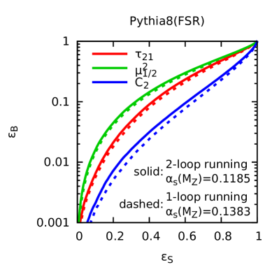
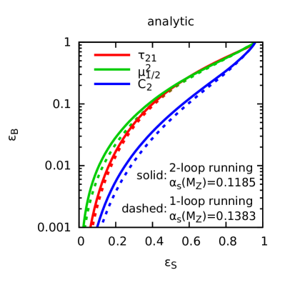
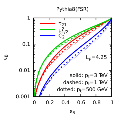
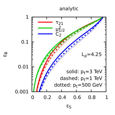
One-loop v. two-loop running coupling.

First, in Sections 4.9 and 5.6, we have used a one-loop running of $\alpha_{s}$, with $\alpha_{s}(M_{Z})=0.1383$, for Pythia simulations, and compared that to analytic calculations including two-loop corrections and using $\alpha_{s}(M_{Z})=0.1185$. In the case of our analytic calculation, this choice is motivated by the fact that two-loop corrections are easily included and we then used the world-average value pdg at the $Z$-boson mass. For the Pythia simulation, we simply kept the default which is a one-loop running.

We could also have run Pythia with a two-loop running of the coupling and impose $\alpha_{s}(M_{Z})=0.1185$. We did not do that in the main text because that can only safely be done with a retuning of other parameters in Pythia (mostly for the non-perturbative effects). It is however interesting to check that this difference in the treatment of the running of the strong coupling does not come with large effects. The result is presented in Fig. 15, where we see that this is indeed a small effect which does not alter in any way the conclusions of this paper. We also see from that figure that the size of the effect is similar in Monte-Carlo simulations and in our analytic predictions.

Note also that another interesting check of our results is to compare our fixed-order results with Pythia simulations also done with a fixed coupling. Although we do not show explicit plots here, this comparison shows similar features as the ones observed with a running-coupling prescription.

Dependence on the jet transverse momentum.

Throughout this paper, we have shown results for jets with a large transverse momentum of 3 TeV. Here, we briefly show that our calculations remain valid for less boosted jets, closer to those used in today’s phenomenological analyses.

In Fig. 16, we show ROC curves obtained from Pythia simulations and our analytic calculations, for three different jet transverse momenta: 3 TeV, 1 TeV and 500 GeV. For this comparison, we have kept the ratio $m/p_{t}$ fixed, i.e. considered a mass of 358, 120 and 60 GeV respectively for each of the three $p_{t}$ scales. We see that the dependence on the jet $p_{t}$ is mild, which is expected since the result only depend on $p_{t}$ through the $p_{t}R$ scale entering in $\alpha_{s}$. Our conclusions are therefore also valid for jets of more moderate transverse momentum. Note that the small differences observed in Pythia simulations between different jet $p_{t}$ are well reproduced by our analytic calculation.

References

- (1) A. Abdesselam et al., Eur. Phys. J. C 71 (2011) 1661 [arXiv:1012.5412 [hep-ph]].
- (2) A. Altheimer et al., J. Phys. G 39 (2012) 063001 [arXiv:1201.0008 [hep-ph]].
- (3) A. Altheimer et al., Eur. Phys. J. C 74 (2014) 3, 2792 [arXiv:1311.2708 [hep-ex]].
- (4) D. Adams et al., Eur. Phys. J. C 75 (2015) 9, 409 [arXiv:1504.00679 [hep-ph]].
- (5) J. M. Butterworth, A. R. Davison, M. Rubin and G. P. Salam, Phys. Rev. Lett. 100 (2008) 242001 [arXiv:0802.2470 [hep-ph]].
- (6) D. Krohn, J. Thaler and L. T. Wang, JHEP 1002 (2010) 084 [arXiv:0912.1342 [hep-ph]].
- (7) S. D. Ellis, C. K. Vermilion and J. R. Walsh, Phys. Rev. D 80 (2009) 051501 [arXiv:0903.5081 [hep-ph]].
- (8) S. D. Ellis, C. K. Vermilion and J. R. Walsh, Phys. Rev. D 81 (2010) 094023 [arXiv:0912.0033 [hep-ph]].
- (9) J. Thaler and K. Van Tilburg, JHEP 1103 (2011) 015 [arXiv:1011.2268 [hep-ph]].
- (10) J. H. Kim, Phys. Rev. D 83 (2011) 011502 [arXiv:1011.1493 [hep-ph]].
- (11) J. Thaler and K. Van Tilburg, JHEP 1202 (2012) 093 [arXiv:1108.2701 [hep-ph]].
- (12) A. J. Larkoski, G. P. Salam and J. Thaler, JHEP 1306 (2013) 108 [arXiv:1305.0007 [hep-ph]].
- (13) A. J. Larkoski, I. Moult and D. Neill, JHEP 1412 (2014) 009 [arXiv:1409.6298 [hep-ph]].
- (14) M. Dasgupta, A. Fregoso, S. Marzani and G. P. Salam, JHEP 1309 (2013) 029 [arXiv:1307.0007 [hep-ph]].
- (15) S. Catani and M. H. Seymour, Nucl. Phys. B 485 (1997) 291 [Nucl. Phys. B 510 (1998) 503] [hep-ph/9605323].
- (16) M. Seymour, http://hepwww.rl.ac.uk/theory/seymour/nlo/
- (17) A. J. Larkoski, S. Marzani, G. Soyez and J. Thaler, JHEP 1405 (2014) 146 [arXiv:1402.2657 [hep-ph]].
- (18) C. W. Bauer, S. Fleming, D. Pirjol and I. W. Stewart, Phys. Rev. D 63 (2001) 114020 [hep-ph/0011336].
- (19) C. W. Bauer and I. W. Stewart, Phys. Lett. B 516 (2001) 134 [hep-ph/0107001].
- (20) C. W. Bauer, D. Pirjol and I. W. Stewart, Phys. Rev. D 65 (2002) 054022 [hep-ph/0109045].
- (21) C. W. Bauer, F. J. Tackmann, J. R. Walsh and S. Zuberi, Phys. Rev. D 85 (2012) 074006 [arXiv:1106.6047 [hep-ph]].
- (22) R. Abbate, M. Fickinger, A. H. Hoang, V. Mateu and I. W. Stewart, Phys. Rev. D 83 (2011) 074021 [arXiv:1006.3080 [hep-ph]].
- (23) A. J. Larkoski, I. Moult and D. Neill, JHEP 1605 (2016) 117 doi:10.1007/JHEP05(2016)117 [arXiv:1507.03018 [hep-ph]].
- (24) I. W. Stewart, F. J. Tackmann and W. J. Waalewijn, Phys. Rev. Lett. 105 (2010) 092002 [arXiv:1004.2489 [hep-ph]].
- (25) J. M. Butterworth, B. E. Cox and J. R. Forshaw, Phys. Rev. D 65 (2002) 096014 [hep-ph/0201098].
- (26) I. W. Stewart, F. J. Tackmann, J. Thaler, C. K. Vermilion and T. F. Wilkason, JHEP 1511 (2015) 072 doi:10.1007/JHEP11(2015)072 [arXiv:1508.01516 [hep-ph]].
- (27) J. Thaler and T. F. Wilkason, JHEP 1512 (2015) 051 doi:10.1007/JHEP12(2015)051 [arXiv:1508.01518 [hep-ph]].
- (28) A. J. Larkoski and I. Moult, Phys. Rev. D 93 (2016) 014017 doi:10.1103/PhysRevD.93.014017 [arXiv:1510.08459 [hep-ph]].
- (29) S. Catani, Y. L. Dokshitzer, M. Olsson, G. Turnock and B. R. Webber, Phys. Lett. B 269 (1991) 432.
- (30) S. Catani, Y. L. Dokshitzer, M. H. Seymour and B. R. Webber, Nucl. Phys. B 406 (1993) 187.
- (31) S. D. Ellis and D. E. Soper, Phys. Rev. D 48 (1993) 3160 [hep-ph/9305266].
- (32) M. Cacciari, G. P. Salam and G. Soyez, Eur. Phys. J. C 72 (2012) 1896 [arXiv:1111.6097 [hep-ph]].
- (33) Y. L. Dokshitzer, G. D. Leder, S. Moretti and B. R. Webber, JHEP 9708 (1997) 001 [hep-ph/9707323].
- (34) M. Wobisch and T. Wengler, In *Hamburg 1998/1999, Monte Carlo generators for HERA physics* 270-279 [hep-ph/9907280].
- (35) See e.g. https://fastjet.hepforge.org/trac/browser/contrib/contribs/Nsubjettiness/tags/2.1.0 for the practical implementation of -subjettiness.
- (36) FastJet Contrib, http://fastjet.hepforge.org/contrib .
- (37) M. Dasgupta, A. Fregoso, S. Marzani and A. Powling, Eur. Phys. J. C 73 (2013) 11, 2623 [arXiv:1307.0013 [hep-ph]].
- (38) M. Dasgupta and G. P. Salam, Phys. Lett. B 512 (2001) 323 [hep-ph/0104277].
- (39) M. Dasgupta, K. Khelifa-Kerfa, S. Marzani and M. Spannowsky, JHEP 1210 (2012) 126 [arXiv:1207.1640 [hep-ph]].
- (40) M. Dasgupta, A. Powling and A. Siodmok, JHEP 1508 (2015) 079 [arXiv:1503.01088 [hep-ph]].
- (41) S. Catani, G. Turnock and B. R. Webber, Phys. Lett. B 272 (1991) 368.
- (42) M. Cacciari, G. P. Salam and G. Soyez, JHEP 0804 (2008) 063 [arXiv:0802.1189 [hep-ph]].
- (43) T. Sjostrand, S. Mrenna and P. Z. Skands, Comput. Phys. Commun. 178 (2008) 852 [arXiv:0710.3820 [hep-ph]].
- (44) M. Bahr, S. Gieseke, M. A. Gigg, D. Grellscheid, K. Hamilton, O. Latunde-Dada, S. Platzer and P. Richardson et al., Eur. Phys. J. C 58 (2008) 639 [arXiv:0803.0883 [hep-ph]].
- (45) R. W. L. Jones, M. Ford, G. P. Salam, H. Stenzel and D. Wicke, JHEP 0312 (2003) 007 [hep-ph/0312016].
- (46) J. Gallicchio and M. D. Schwartz, Phys. Rev. Lett. 107 (2011) 172001 [arXiv:1106.3076 [hep-ph]].
- (47) A. J. Larkoski, J. Thaler and W. J. Waalewijn, JHEP 1411 (2014) 129 [arXiv:1408.3122 [hep-ph]].
- (48) G. Aad et al. [ATLAS Collaboration], Eur. Phys. J. C 74 (2014) 8, 3023 [arXiv:1405.6583 [hep-ex]].
- (49) A. J. Larkoski and J. Thaler, JHEP 1309 (2013) 137 [arXiv:1307.1699 [hep-ph]].
- (50) A. J. Larkoski, S. Marzani and J. Thaler, Phys. Rev. D 91 (2015) 11, 111501 [arXiv:1502.01719 [hep-ph]].
- (51) S. Catani, B. R. Webber and G. Marchesini, Nucl. Phys. B 349 (1991) 635.
- (52) Y. L. Dokshitzer, V. A. Khoze and S. I. Troian, Phys. Rev. D 53 (1996) 89 [hep-ph/9506425].
- (53) A. Banfi, G. P. Salam and G. Zanderighi, JHEP 0503 (2005) 073 [hep-ph/0407286].
- (54) K. A. Olive et al. [Particle Data Group Collaboration], Chin. Phys. C 38 (2014) 090001. doi:10.1088/1674-1137/38/9/090001