Ground state of the holes localized in II-VI quantum dots
with Gaussian potential profiles

Abstract

We report on the theoretical study of the hole states in II-IV quantum dots of a spherical and ellipsoidal shape, described by a smooth potential confinement profiles, that can be modelled by a Gaussian functions in all three dimensions. The universal dependencies of the hole energy, $g$-factor and localization length on a quantum dot barrier height, as well as the ratio of effective masses of the light and heavy holes are presented for the spherical quantum dots. The splitting of the four-fold degenerate ground state into two doublets is derived for anisotropic (oblate or prolate) quantum dots. Variational calculations are combined with numerical ones in the framework of the Luttinger Hamiltonian. Constructed trial functions are optimized by comparison with the numerical results. The effective hole $g$–factor is found to be independent on the quantum dot size and barrier height and is approximated by simple universal expression depending only on the effective mass parameters. The results can be used for interpreting and analyzing experimental spectra measured in various structures with the quantum dots of different semiconductor materials.

I Introduction

Quantum dots (QDs), sometimes referred to as nanocrystals (NCs) in literature, are systems with good prospects for nanotechnology. Physically, the QDs are tiny semiconductor nanoparticles which are formed in various dielectric or semiconductor matrices by different methods. Among them, the basic ones are the chemical synthesis and epitaxy used to fabricate, respectively, the colloidal and epitaxial QDs. Depending on the used semiconductors and the fabrication methods, the QDs can have various shapes and sizes. Carrier localization in the QDs makes interaction between charge carriers more efficient as compared with bulk materials, and many effects that are weak in bulk materials become observable. Thus, the development of new methods of the calculation of the wave functions and energy spectra of charge carriers is very important for designing the QD structures.

The incentive to our study was the renewed interest in II-VI QDs for various applications. In particular, the epitaxial CdSe/Zn(S,Se) QDs have been successfully used as an active region in laser heterostructures pumped optically or by an electron beam. Ivanov2013 ; Sorokin2015 Besides, they have been recognized as promising candidates for room temperature single photon emission and production of photon pairs due to strong carrier confinement and distinct biexciton performance Strauf ; Tribu ; Fedorych . The self-formation of these nanostructures takes place when a CdSe insertion of a fraction monolayer (ML) thickness is deposited within a Zn(S,Se) matrix. Previously, this insertion was considered as a disordered quantum well, where the nano-islands with high Cd content, $x$, are formed within the matrix with lower $x$. Klochikhin ; Peranio2000 Thorough transmission electron microscopy (TEM) studies Litvinov2008 , however, have shown that the Cd content in the Cd-rich nano-islands can be as high as 80% in the center, decreasing towards the periphery, while the Cd concentration in the surrounding area approaches 20% only. The average lateral sizes of the nano-islands are about 5 nm, while the sizes in the growth direction are somewhat smaller. These findings make it possible to consider the nano-islands as oblate ellipsoidal QDs. Such an asymmetric shape influences the energy splitting of both exciton and biexciton states in the single CdSe/ZnSe QD Kulakovskii99 , that is important for the generation of the entangled photon pairs. The CdSe/Zn(S,Se) structures exhibited the long-lived electron spin coherence, related likely to the three-dimensional localization potential Syperek . Recently, it has been demonstrated that at a certain deposited amount of CdSe the nano-islands can be quite isolated Reznitsky2015 . Importantly, the change of the concentration between the dot and barrier regions in the epitaxial CdSe/Zn(S,Se) QDs is not abrupt but gradual due to diffusion and segregation processes.

The II-VI QDs with such a gradual composition variation are expected to demonstrate an improved radiative emission. Indeed, for a long time, the biexciton performance of the chemically synthesized colloidal QDs was suffering from a high rate of non-radiative Auger recombination. To overcome this problem colloidal CdSe-based nanocrystal heterostructures with gradually changing composition were synthesized and reported in Ref. Nasilowski15, . The non-radiative Auger processes are suppressed in such structures due to smoothing of the confining potential. Cragg2010 ; Garcia-Santamaria2011 ; Bae ; Climente2012 Further progress in analysis of optical phenomena in the II-VI QDs and manufacturing the efficient nano emitters of quantum light requires the elaborated model description of quantum states in the ellipsoidal QDs with smooth potential profile. Among variety of theoretical methods, including atomistic tight-binding Korkusinski10 ; Zieli?nski15 or pseudo-potential calculations Bester10 , and $\bm{kp}$-theory, the latter provides a reasonable compromise between the accuracy and computational complexity. The $\bm{kp}$ method is particularly suitable for nanostructures with a smooth potential profile, where interface effects play a minor role.

In the most simple effective mass model of non-degenerate parabolic band, various kinds of confinement potentials for QDs were theoretically studied: abrupt potential with infinite and finite barriers, Efros82 ; Brus ; Marin ; Pellegrini ; Schooss94 ; Rego97 parabolic potential Que ; Xie2006 and various kinds of smooth potential with finite height. Adamowski ; Ciurla ; Xie2009 ; Szafran2001 The parabolic potential was also shown to be a good approximation for the in-plane smooth profile of the lens-shaped self-assembled QDs.Wojs1996 However, to describe properly the energy spectra of the holes confined in QDs, one has to take into account the complex structure of the valence band. In widely used semiconductors (including II-VI), the top of the valence band is four-fold degenerate and has $\Gamma_{8}$ symmetry and can be described by the Luttinger Hamiltonian. Luttinger The fine energy structure of the hole states defines the selection rules for inter-band transitions. Moreover, the Zeeman splitting in the external magnetic field is determined by the light and heavy holes splitting and mixing. Rego97 ; Kubisa11 ; Semina2015 Therefore, the understanding of the characteristic properties of the hole states in QDs is important for designing the structures with required optical properties.

For the spherical NCs Efros89 ; Xia89 ; EkimovJOSA93 and the disk-like QDs Rego97 modelled by abrupt potential with infinite barrier, it was shown, that the mixing of the heavy and light hole states can significantly modify the energy spectrum and the wave function of the hole ground state, as well as its splitting which can be caused by the anisotropy of QD shape, intrinsic crystal field, and applied magnetic field.EfrosPRB96 Later, the full multiband ${\bm{k}}\cdot{\bm{p}}$ modelling was developed for spherical NCsEfrosPRB98 and NC heterostructures with abrupt potential barriers,Jaskolski98 as well as for the pyramidal and disk-shaped epitaxial QDs.Pryor98 ; Stier99 ; Tadic2002 The models of parabolic potential with valence band degeneration taken into account were used for QDs of different shapes, Rinaldi ; Rodina2010 ; Semina2015 not only within effective mass approach but also as the modelling tool along with more elaborated atomistic calculations.Korkusinski2013 However, to the best of our knowledge, the QDs with smooth but finite height potential confinement in all three spatial dimensions have been considered only within single band effective mass approximation so far. This simplified approximation can hardly be used for both epitaxial CdSe/ZnSe and colloidal CdSe/CdS QDs with gradually varying composition. Peranio2000 ; Litvinov2008 ; Nasilowski15

In present paper we consider QDs with a shape which is close to either spherical or ellipsoidal one and a smooth potential profile which can be described by the Gaussians in all three spatial directions. We focus on the characteristics of the hole localized in such potential taking into account the complex valence band structure in the framework of the Luttinger Hamiltonian. It is shown that the properties of the holes localized in a smooth potential profiles, e.g. energy splittings caused by the shape anisotropy or external magnetic field, might be very different from the properties of the holes localized in a box–like QDs with abrupt potential barriers.

The paper is organized as follows: in Section II we introduce the regularities of our problem on the most intuitive example of the material with single band isotropic parabolic dispersion. In Section III we move on to the characteristic properties of the hole localized in spherically symmetric quantum dot with the top of valence band that can be described by the Luttinger Hamiltonian. In Sections IV and V we consider the hole ground state splitting due to the anisotropy of the QD potential, crystal field, and external magnetic field. In the end we summarize our results.

II Localization of a particle in QD with parabolic or Gaussian profile: single band approximation

To introduce the specifics of the carriers localization in the quantum dots described by the smoothly varying spatial potential $V({\bm{r}})$ ($r$ is the radial coordinate) we consider the the Schrödinger equation $[\hat{H}+V({\bm{r}})]\Psi=E\Psi$ with the single band isotropic effective mass Hamiltonian

$$\hat{H}=\frac{\hbar^{2}\hat{k}^{2}}{2m^{*}}\,.$$ (1)

Here ${\bm{k}}=-{\mathrm{i}}{\bm{\nabla}}$ is the wave vector operator and $m^{*}=m_{\rm e(h)}$ is the electron (hole) effective mass. We consider the cases of the spherical symmetry $V({\bm{r}})=V({r})$ and axial symmetry $V({\bm{r}})=V(\rho,z)$ potentials, where $r^{2}=x^{2}+y^{2}+z^{2}=\rho^{2}+z^{2}$, $x,y,z$ – are Cartesian coordinates.

II.1 Spherically symmetric QD

We start with the spherical parabolic (harmonic oscillator) potential, that is the limiting case for the Gaussian potential

$$V_{0}(r)=\frac{\kappa}{2}r^{2},$$ (2)

where $\kappa$ is the spring constant. In the framework of single band effective mass approximation the exact solutions of the problem with such potential are well known. The spherical oscillator wave functions can be easily found as:

$$\Psi_{nlm}({\bf r})=R_{nl}(r)Y_{lm}(\Theta)\,,\\ R_{nl}(r)=\frac{1}{L^{3/2+l}}\left[\frac{2n!}{\Gamma\left(n+l+3/2\right)}\right]^{1/2}r^{l}\times\\ \times\exp\left[-\frac{r^{2}}{2L^{2}}\right]L_{n}^{l+1/2}\left[\frac{r^{2}}{L^{2}}\right]\,,$$ (3)

and correspond to the equidistant eigen energies

$$E_{N}=\hbar\omega(N+3/2)\,\quad N=2n+l=0,1,2.....$$ (4)

Here $\omega=\sqrt{\kappa/m^{*}}$ and $L=\sqrt{\hbar/m^{*}\omega}$ are the characteristic oscillator frequency and oscillator length, respectively, $n,l$ and $m$ are principal, orbital and magnetic quantum numbers, respectively, $Y_{lm}$ are the spherical angular harmonics Edmonds and $L_{n}^{l+1/2}$ are the generalized Laguerre polynomials polynoms . The ground state energy and radial wave function of the particle localized in $V_{0}(r)$ are characterized by $n=0$, $l=0$ and given by

$$E_{0}=\frac{3}{2}\hbar\omega=\frac{3}{2}\frac{\hbar^{2}}{m^{*}L^{2}}$$ (5)

and

$$R_{0}(r)=\frac{2}{\pi^{1/4}L^{3/2}}\exp\left[-\frac{r^{2}}{2L^{2}}\right]\,.$$ (6)

The parabolic potential describes the QD with smooth profile, however yet it does not permit us to consider the QDs with the finite potential barrier outside the dot. To do so we consider the potential of the Gaussian form

$$V_{\text{G}}(r)=V_{\text{off}}\left(1-\exp\left[-\frac{r^{2}}{a^{2}}\right]\right),$$ (7)

where $V_{\text{off}}$ is the energy step (band-offset) between the QD center and the surrounding medium, determined as $r>3a$, while $a$ can be used as the rough estimation of the QD radius. Near the QD center, at $r\ll a$, the Gaussian potential can be approximated as parabolic $V_{\text{G}}(r)\approx V_{0}(r)$ with the spring constant $\kappa=2V_{\text{off}}/a^{2}$. To simplify the comparison of the potentials characterized by the same spring constant $k$ at the QD center and different potential barriers $V_{\text{off}}$, we chose the parameters of the single band parabolic problem – the ground state energy $E_{0}$ and the oscillator length $L$ – as the energy and length units for all QDs. In these units the parabolic and Gaussian potentials take the form

$$\tilde{V}_{0}(\tilde{r})=V_{0}(r/L)/E_{0}=\frac{1}{3}\tilde{r}^{2}\,,$$ (8)

$$\tilde{V}_{\text{G}}(\tilde{r})=V_{\text{G}}(r/L)/E_{0}=\tilde{V}_{\text{off}}\left(1-\exp\left[-\frac{\tilde{r}^{2}}{3\tilde{V}_{\text{off}}}\right]\right),$$ (9)

where $\tilde{V}_{\text{off}}=V_{\text{off}}/E_{0}$ and $\tilde{r}=r/L$. Note that the spring constant is not included explicitly in eqs. (8) and (9). It is, however, contained in expressions for our units $L$ and $E_{0}$. This fact allows us to obtain the universal dependence of the localized particle wave function and energy spectrum on $\tilde{V}_{\text{off}}$. The dimensionless parabolic and Gaussian potentials with different $\tilde{V}_{\text{off}}$ are shown in Fig. 1(a), the chosen values of $\tilde{V}_{\text{off}}$ correspond to characteristic radii $\tilde{a}=a/L=\sqrt{3\tilde{V}_{off}}\approx 1.73,~{}2.45$ and $4.9$. Vertical dashed lines show the characteristic radii $\tilde{a}$ for shallowest dots with $\tilde{V}_{\text{off}}=1$ and $2$, for $\tilde{V}_{\text{off}}=8$ the value of $\tilde{a}$ lays outside the scale of the figure, the parabolic potential has the infinite effective radius.

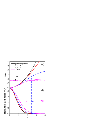
Figure 1: (Color online) (a) Dimensionless parabolic and Gaussian potentials with $\tilde{V}_{\text{off}}=8;2;1$. (b) Probability distribution $\tilde{R}_{0}^{2}(\tilde{r})$ for different $\tilde{V}_{\text{off}}$; Vertical dashed lines on (a) and (b) show the characteristic radii $\tilde{a}$ for $\tilde{V}_{\text{off}}=1$ and $2$ and $2\tilde{a}$ for $\tilde{V}_{\text{off}}=1$. Horizontal dotted lines on panel (a) show the potential depth $\tilde{V}_{\text{off}}$ and energy level $E/E_{0}$ for $\tilde{V}_{\text{off}}=1$.

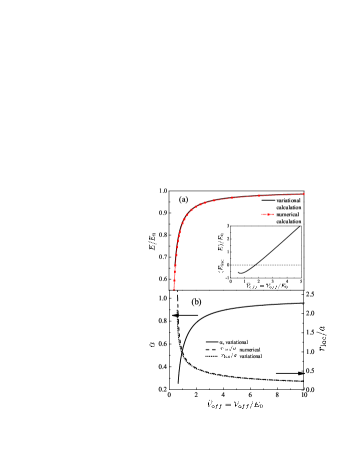
Figure 2: (Color online) (a) Dependence of the hole ground state energy $E/E_{0}$ on the $\tilde{V}_{\text{off}}=V_{\text{off}}/E_{0}$, the inset shows the dimensionless difference between the localization energy and particle energy; (b) Dependencies of the variational parameter $\alpha$ and the localization radius $r_{\rm loc}/a$ on $\tilde{V}_{\text{off}}$.

Since no exact solution exists for the particle in Gaussian potential, we found the wave function and energy of the ground state by two methods - numerical and variational. Numerical solution can be found by expanding the radial wave functions over the basis of the oscillator functions (3) and diagonalizing the resulting matrix.

To obtain the ground state energy by the variational procedure we chose the dimensionless probe function $\tilde{R}_{0}(\tilde{r})=R_{0}(r/L)L^{3/2}$ in the form:

$$\tilde{R}_{0}=\frac{2\alpha^{3/4}}{\pi^{1/4}}\exp\left[-\frac{\alpha\tilde{r}^{2}}{2}\right]\,$$ (10)

with $\alpha$ being the only trial parameter. With the probe function (10) we have the following expression for the particle ground state energy as a function of $\alpha$:

$$E(\alpha)/E_{0}=\frac{\alpha}{2}+\tilde{V}_{\text{off}}-\frac{3\sqrt{3}\alpha^{3/2}\tilde{V}^{5/2}_{\text{off}}}{\left(1+3\alpha\tilde{V}_{\text{off}}\right)^{3/2}}.$$ (11)

Figure 1(b) shows the dimensionless probability distribution $\tilde{R}_{0}^{2}(\tilde{r})$ for Gaussian QDs with different $\tilde{V}_{\text{off}}$ and for parabolic QDs. Figure 2(a) shows the dependences of the dimensionless ground state energy $E/E_{0}$ on the $\tilde{V}_{\text{off}}=V_{\text{off}}/E_{0}$ and Fig. 2(b) shows the dependence of the minimizing value of trial parameter $\alpha$ on $\tilde{V}_{\text{off}}$. Panels (a) of figs. 1 and 2 demonstrate, that with the increase of $\tilde{V}_{\text{off}}$ the ground state energy and the wave function in Gaussian potential tend to those of the harmonic oscillator. While with decrease of $\tilde{V}_{\text{off}}$ the quantization energy $E/E_{0}$ decreases, the localization energy $E_{\rm loc}/E_{0}=(V_{\rm off}-E)/E_{0}$ also decreases and becomes smaller than $E$ for $\tilde{V}_{\text{off}}<2$ (see inset in fig. 2(a)). The bound state exists up to $\tilde{V}_{\text{off}}\approx 0.55$ as it is shown by the numerical calculation; the variational calculation gives the bound state up to $\tilde{V}_{\text{off}}\approx 0.65$.

The localization of the particle inside the QD can be characterized by the localization radius $\tilde{r}_{\rm loc}=r_{\rm loc}/L=\sqrt{<\tilde{r}^{2}>}=\sqrt{\int_{0}^{\infty}\tilde{R}_{0}^{2}\tilde{r}^{4}d\tilde{r}}$. We find $\tilde{r}_{\rm loc}\approx 1.23$ for the parabolic potential and $\tilde{V}_{\text{off}}=8$, and $\tilde{r}_{\rm loc}\approx 1.39$ and $\tilde{r}_{\rm loc}\approx 1.76$ for $\tilde{V}_{\text{off}}=2$ and $\tilde{V}_{\text{off}}=1$, respectively. One can see that $\tilde{r}_{\rm loc}\approx 1.76$ only slightly exceeds the effective radius $\tilde{a}\approx 1.73$ for $\tilde{V}_{\text{off}}=1$ and $\tilde{r}_{\rm loc}<\tilde{a}$ for $\tilde{V}_{\text{off}}=2$ and higher potential barriers. In spite of the very small localization energy in the dots with $\tilde{V}_{\text{off}}<2$, the probability density $|\tilde{R}_{0}(\tilde{r})|^{2}$ is well localized inside these dots up to $\tilde{V}_{\text{off}}=1$. The dependence of $r_{\rm loc}/a=\tilde{r}_{\rm loc}/\tilde{a}$ on $\tilde{V}_{\text{off}}$ is also shown in Fig. 2(b). Note that the radius $2a$ corresponds to the point where the Gaussian potential saturates: $V_{\rm G}(2a)\approx V_{\rm off}$. For the probe function (10), $\tilde{r}_{\rm loc}=\sqrt{1.5/\alpha}$ and $r_{\rm loc}/a=\tilde{r}_{\rm loc}/\tilde{a}=\sqrt{1/(2\alpha\tilde{V}_{\text{off}})}$.

II.2 Axially symmetric non-spherical QD

Now we consider ellipsoidal axially symmetric QDs, where parabolic confinement potential can be written as:

$$V_{p}^{a}(r,z,\mu)=\frac{\kappa_{\rho}}{2}\rho^{2}+\frac{\kappa_{z}}{2}z^{2}=V_{0}(r)+\Delta V_{p}^{a}(\rho,z,\mu)\,,$$ (12)

$$\Delta V_{p}^{a}(\rho,z,\mu)=\kappa\mu\left(z^{2}-\frac{1}{3}r^{2}\right).$$ (13)

Here the average spring constant is $\kappa=(2\kappa_{\rho}+\kappa_{z})/3$ and we introduce the QD anisotropy parameter as

$$\mu=\frac{3}{2}\frac{(\kappa_{z}/\kappa_{\rho}-1)}{(\kappa_{z}/\kappa_{\rho}+2)}=\frac{(\kappa_{z}-\kappa_{\rho})}{2\kappa}.$$ (14)

One can see that $\mu>0$ corresponds to the case $\kappa_{z}>\kappa_{\rho}$ and thus describes stronger confinement along $z$ direction (oblate QD). In the opposite case of $\mu<0$ the confinement is stronger in $xy$ plane (prolate QD). Note that the Eq. (12) is exact. It follows from (14) that

$$\kappa_{\rho}=\kappa\left(1-\frac{2}{3}\mu\right),~{}\kappa_{z}=\kappa\left(1+\frac{4}{3}\mu\right)\,$$ (15)

and the condition that $k_{\rho,z}\geq 0$ leads to only $-3/4\leq\mu\leq 3/2$ having physical sense.

The exact solutions for the axially symmetric harmonic potential (12) are also well known. We introduce parameters $L_{x},~{}L_{y},~{}L_{z}$ as oscillator lengths along $x,~{}y,~{}z$ axes correspondingly, and note that in the axially-symmetric potential $L_{x}=L_{y}=L$. In this case, the wave functions can be calculated from the Schrödinger equation for axially-symmetric harmonic oscillator:

$$\Psi_{n_{x},n_{y},n_{z}}({x,y,z})=\frac{1}{\sqrt{2^{n_{x}+n_{y}+n_{z}}}n_{x}!n_{y}!n_{z}!}\frac{\pi^{-3/4}}{L\sqrt{L_{z}}}\times\\ \times H_{n_{x}}\left[\frac{x}{L}\right]H_{n_{y}}\left[\frac{y}{L}\right]H_{n_{z}}\left[\frac{z}{L_{z}}\right]\exp\left[-\frac{x^{2}+y^{2}}{2L^{2}}-\frac{z^{2}}{2L_{z}^{2}}\right]\,,$$ (16)

and correspond to the equidistant eigen energies

$$E_{n_{x},n_{y},n_{z}}=\hbar\omega(n_{x}+n_{y}+2)+\hbar\omega_{z}(n_{z}+1),\\ \quad n_{x},n_{y},n_{z}=0,1,2.....$$ (17)

Here $H_{n}\left[x\right]$ are Hermite polynomials polynoms , $\omega=\sqrt{k_{\rho}/m}$, $\omega_{z}=\sqrt{k_{z}/m}$ and $L=\sqrt{\hbar/m\omega},~{}L_{z}=\sqrt{\hbar/m\omega_{z}}$. For the ground state energy we obtain:

$$E_{0}^{a}=\frac{1}{2}\left[\frac{2\hbar^{2}}{mL^{2}}+\frac{\hbar^{2}}{mL_{z}^{2}}\right]=\\ =\frac{2E_{0}}{3}\left[\sqrt{1-2\mu/3}+\frac{1}{2}\sqrt{1+4\mu/3}\right]\approx E_{0}\left[1-\frac{\mu^{2}}{9}\right]\,.$$ (18)

One can see that (18) containes no linear on $\mu$ correction to the ground state energy. The same result can be readily observed by treating $\Delta V_{p}^{a}(\rho,z,\mu)$ as perturbation.

We consider the anisotropic Gaussian potential with axial symmetry in the form

$$V_{G}^{a}(r,z,\mu)=V_{\text{off}}\left(1-\exp\left[-\frac{x^{2}+y^{2}}{a_{x}^{2}}-\frac{z^{2}}{a_{z}^{2}}\right]\right)\,.$$ (19)

The ground state energy of the particle in such potential can be found numerically by expanding the wave functions over the basis of the oscillator functions (16), diagonalizing the resulting matrix. The anisotropy can also be considered in the framework of the perturbation theory by two ways. One way is to find the isotropic and anisotropic part of the Hamiltonian Eq. (19) as it was done in (12):

$$V_{G}^{a}(r,z,\mu)=V_{\text{off}}\left(1-\exp\left[-\frac{x^{2}+y^{2}}{a_{x}^{2}}-\frac{z^{2}}{a_{z}^{2}}\right]\right)\approx\\ \approx V_{G}(r)+\Delta V_{p}^{a}(r,z,\mu)\,,\\ \Delta V_{G}^{a}(r,z,\mu)=\exp\left[-\frac{r^{2}}{a^{2}}\right]\Delta V_{p}^{a}(r,z,\mu)\,,$$ (20)

where $a={\sqrt{3}a_{x}a_{z}}/{\sqrt{a_{x}^{2}+2a_{z}^{2}}}$. The effective spring constants are introduced by analogy with the spherical QD: $\kappa_{\rho}=2V_{\text{off}}/a_{x}^{2}$ and $\kappa_{z}=2V_{\text{off}}/a_{z}^{2}$. Anisotropy parameter $\mu$ is defined in the same way as for the parabolic potential (14). Approximate expansion (20) keeps only terms linear on $\mu$ and is applicable for $\mu<1$. Again, the first order energy correction to the $s$ symmetry ground state for the perturbation $\Delta V_{G}^{a}(r,z,\mu)$ vanishes. Using numerical approach for $\mu<1$ we found that the shift of the ground state energy in the anisotropic Gaussian potential can be described as $E^{a}(\mu)\approx E^{a}(\mu=0)\left[1-{\mu^{2}}/{9}\right]$ by analogy with expression (18).

Alternatively, the anisotropy of the Gaussian potential can be treated by replacing the coordinates as $x\longrightarrow x(a_{x}/a)$ and $z\longrightarrow z(a_{z}/a)$. The potential energy becomes isotropic in the new coordinates. However, the kinetic energy operator $\hat{H}$ in acquires the additional term

$$\Delta\hat{H}^{\rm a}_{\rm k}=\frac{2\mu}{3}\frac{\hbar^{2}}{2m}\left[\hat{k}^{2}-3\hat{k}_{z}^{2}\right]\,.$$ (21)

Again, the linear on $\mu$ energy correction to the ground state from $\Delta\hat{H}^{\rm a}$ vanishes.

III Spherical symmetry problem for the $\Gamma_{8}$ valence band.

We consider now the hole in four-fold degenerate $\Gamma_{8}$ valence subband for semiconductors with large spin-orbit splitting. Luttinger Hamiltonian for such semiconductors in spherical approximation can be written Luttinger ; Gelmont71 as

$$\hat{H}_{\rm L}=\frac{\hbar^{2}}{2m_{0}}\left[\left(\gamma_{1}+\frac{5}{2}\gamma\right)\hat{k}^{2}-2\gamma(\hat{\bm{k}}{\bm{j}})^{2}\right]\,.$$ (22)

Here $m_{0}$ is the free electron mass, ${\bm{j}}$ is the hole internal angular momentum operator for $j=3/2$, $\gamma_{1}$ and $\gamma=(2\gamma_{2}+3\gamma_{3})/5$ are Luttinger parameters related to the light and heavy hole effective masses as $m_{lh,hh}=m_{0}/(\gamma_{1}\pm 2\gamma)$.

The first energy level of holes in a spherical QDs in a semiconductor with degenerate $\Gamma_{8}$ valence subband is $1S_{3/2}$ state.Efros89 ; EkimovJOSA93 It has total angular momentum ${\bm{J}}={\bm{j}}+{\bm{l}}$ with $J=3/2$ and is four-fold degenerate with respect to its projection on the $z$ axis. The wave functions of this state can be written asGelmont71 ; note

$$\Psi_{M}=2\sum_{l=0,2}(-1)^{M-3/2}(i)^{l}R_{l}(r)\times\\ \times\sum_{m+\mu=M}\left(\begin{array}[]{ccc}l&3/2&3/2\\ m&\mu&-M\end{array}\right)Y_{l,m}u_{\mu}\,,$$ (23)

where $\left({}_{m~{}n~{}p}^{i~{}~{}k~{}~{}l}\right)$ are the Wigner 3j-symbols, and $u_{\mu}$ ($\mu=\pm 1/2,\pm 3/2$) are the Bloch functions of the four-fold degenerate valence band $\Gamma_{8}$ that can be found in Ref. Ivchenko, . The radial wave functions $R_{0}$ and $R_{2}$ in Eq. (23) are normalized: $\int(R_{0}^{2}+R_{2}^{2})r^{2}dr=1$ and satisfy the system of differential equations (6) from Gelmont71, ; Rodina2010, , where the QD potential $V(r)$ instead of the Coulomb one is taken. Below we find $R_{0}$ and $R_{2}$ by numerical and variational methods.

III.1 Numerical method

To calculate numerically the energy spectrum and eigen wave functions of the hole in parabolic or Gaussian quantum dot numerically we follow the approach described in Refs. Balderesci70, ; Balderesci73, . We diagonalize the hole Hamiltonian matrix Gelmont71 calculated on non-orthogonal basis, consisting of Gaussian functions times the polynomials of the lowest power, which behave correctly at $r=0$:

$$R_{0}=\sum\limits_{i=1}^{N_{\text{max}}=80}A_{i}\exp\left(-\alpha_{i}\tilde{r}^{2}\right),\\ ~{}R_{2}=\sum\limits_{i=1}^{N_{\text{max}}=80}B_{i}\tilde{r}\exp\left(-\alpha_{i}\tilde{r}^{2}\right).$$ (24)

Here $A_{i}$ and $B_{i}$ are coefficients which are to be found by the diagonalization of the Hamiltonian matrix, $\alpha_{i}$ are chosen in the form of geometrical progression from $10^{-6}$ to $10^{3}$. The convergence of the calculation was controlled by modifying the basis (24): changing $\alpha_{i}$ and $N_{\text{max}}$. The calculation was believed to be converged if the basis modification did not change the result. Rather large $N_{\text{max}}$ as compared with Balderesci70 is necessary to obtain reliable results in case of $\beta\rightarrow 0$, here $\beta=m_{lh}/m_{hh}$ is light to heavy hole effective mass ratio. For the limiting case $\beta=1$, all $B_{i}=0$ with a good accuracy and the use of the basis (24) gives the same results as the use of the basis (3). For $\beta\rightarrow 0$ numerically calculated hole radial functions satisfy the exact differential condition: Gelmont71

$$\frac{dR_{0}}{dr}+\frac{dR_{2}}{dr}+\frac{3}{r}R_{2}=0\,.$$ (25)

with a good accuracy.

III.2 Variational method

We chose the trial functions $R_{0}$ and $R_{2}$ for the arbitrary value of $\beta$ allowing them to satisfy the hole Hamiltonian Gelmont71 in two limits $\beta=1$ and $\beta=0$. If $\beta=1$, the limiting case of the simple band dispersion is realized, and for the ground state the probe radial functions should be chosen as $R_{2}=0$ and $R_{0}$ as given by (10). The exact solution for $\beta=0$ is not known, however, the functions $R_{0}$ and $R_{2}$ must satisfy (25). Using these conditions and comparing the resulting functions with the numerically found solutions we arrived at:

$$R_{2}(r)=\frac{C}{L^{3/2}}\cdot\frac{\alpha\tilde{r}^{2}}{2}\left[\exp\left(-\frac{\alpha\tilde{r}^{2}}{2}\right)-\alpha_{2}\exp\left(-\frac{\alpha\beta^{0.3}\tilde{r}^{2}}{2}\right)\right]\,,\\ R_{0}(r)=\frac{C}{L^{3/2}}\cdot\frac{3}{2}\left[\exp\left(-\frac{\alpha\tilde{r}^{2}}{2}\right)+\alpha_{0}\exp\left(-\frac{\alpha\beta^{0.3}\tilde{r}^{2}}{2}\right)\right]-\\ -R_{2}(r)\,,$$ (26)

where $\alpha$, $\alpha_{0}$ and $\alpha_{2}$ are the trial parameters and $C$ is the normalization constant. The oscillator length $L$ is defined as for the single band with heavy hole effective mass $m_{hh}$ and $\tilde{r}=r/L$. Note, that taking $\alpha_{0}=\beta^{3/2}$ and $\alpha_{2}=\beta^{2}$ and using $\beta^{0.5}$ instead of $\beta^{0.3}$ in the second exponent in $R_{0}$ and $R_{2}$ we arrive to the trial function used in Ref. Rodina2010, for the parabolic confinement potential.

III.3 Results: ground state energy and radial wave functions

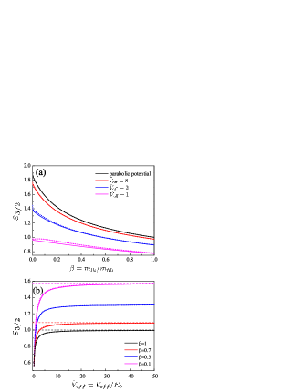
Figure 3: (Color online) Dimensionless ground state energy $\varepsilon_{3/2}$ of the hole as the function of $\beta$ for parabolic potential and Gaussian potential with $\tilde{V}_{\text{off}}=8;2;1$ (a) and as the function of $\tilde{V}_{\text{off}}$ for $\beta=0.1;0.3;0.7;1$ (b). Solid lines correspond to numerical calculation, dotted lines, to variational calculation. Dashed lines on panel (b) indicate the energy in the limit of harmonic oscillator for respective values of $\beta$ .

Figure 4: (Color online) Ratio of the localization radii and the characteristic dot radii, $r_{\rm loc}/a$, the function of $\beta$ for parabolic potential and Gaussian potential with $\tilde{V}_{\text{off}}=8;2;1$ (a) and as the function of $\tilde{V}_{\text{off}}$ for $\beta=0.1;0.3;0.7;1$ (b). Solid lines correspond to numerical calculation, dotted lines, to variational calculation.

Figure 5: (Color online) Dependencies of the variational parameters $\alpha$ (a), $\alpha_{0}(1-\beta)$ (b) and $\alpha_{2}$ (c) on $\beta$ for parabolic potential and $\tilde{V}_{\text{off}}=8;2;1$ and dependencies of the variational parameter $\alpha$ on $\tilde{V}_{\text{off}}$ for $\beta=0.1;0.3;0.7;1$ (d).

The ground state energy, $E_{1S_{3/2}}(\beta)$, is expressed in the units of $E_{0}$ (with $m^{*}=m_{\rm h}$) as follows:

$$E_{1S_{3/2}}(\beta)=\frac{3}{2}\frac{\hbar^{2}}{m_{h}L^{2}}\epsilon_{3/2}(\beta)=E_{0}\epsilon_{3/2}(\beta)\,.$$ (27)

The dimensionless function $\epsilon_{3/2}(\beta)$ calculated variationally and numerically is shown in Fig. 3(a) for the parabolic potential and for Gaussian potential with $\tilde{V}_{\text{off}}=8;2;1$. Fig. 3(b) shows $\epsilon_{3/2}$ as a function of $\tilde{V}_{\text{off}}$ for $\beta=0.1;0.3;0.7;1$. There is a good matching between two methods demonstrating the high accuracy of the variational method, which slightly decreases only for very shallow dot potential (small $\tilde{V}_{\text{off}}$ or very small $\beta$). This fact allows us to validate our choice of the trial function in the form (26). The critical value of $\tilde{V}_{\text{off}}$ defining the appearance of the hole bound state increases with the decrease of $\beta$. Figures 4 (a) and (b) show the dependencies of the ratio $r_{\rm loc}/a$ on $\tilde{V}_{\text{off}}$ and $\beta$, localization radius, $r_{\rm loc}$, is defined as $r_{\rm loc}=\sqrt{<r^{2}>}=\sqrt{\int_{0}^{\infty}({R}_{0}^{2}+{R}_{2}^{2})r^{4}dr}$. Fig. 5 shows the dependencies of the variational parameters $\alpha$, $\alpha_{0}(1-\beta)$ and $\alpha_{2}$ on $\beta$ for $\tilde{V}_{\text{off}}=8;2;1$.

IV Anisotropic splitting of the hole ground state

In this section we consider the hole states in the ellipsoidal QDs with $V(\bm{r})$ given by Eq. (12) and by Eq. (19). Additionally, we consider the effect of the internal crystal field in wurtzite semiconductors, for example CdSe, in the framework of the quasi-cubic approximation. The respective addition to the Hamiltonian is described by $\hat{V}^{\rm cr}=\Delta_{\rm cr}(5/8-j_{z}^{2}/2)$, where $\Delta_{\rm cr}$ is the energy splitting of the light hole and heavy hole valence band edge states in the bulk semiconductor.BirPikus

The internal crystal field in wurtzite semiconductors and the axial anisotropy of the confinement potential lifts the degeneracy of the $1S_{3/2}$ ground hole states in the quantum dot. The four-fold degenerate hole state is split into two doublets with $|M|=3/2$ and $|M|=1/2$:

$$E_{1S_{3/2},~{}M}=E_{1S_{3/2}}^{a}+\frac{\Delta}{2}\left[\frac{5}{4}-M^{2}\right]\,,\\$$ (28)

where $\Delta=\Delta_{\rm int}+\Delta E^{\rm a}$, $\Delta_{\rm int}$ describes the effect of the internal crystal field, $\Delta E^{\rm a}=E_{1S_{3/2},~{}1/2}-E_{1S_{3/2},~{}3/2}$ and $E_{1S_{3/2}}^{a}=(E_{1S_{3/2},~{}1/2}+E_{1S_{3/2},~{}3/2})/2$, describe the hole ground state splitting and the energy shift induced by the QD anisotropy. We calculate $\Delta_{\rm int}$, $\Delta E^{\rm a}$, and $E_{1S_{3/2}}^{a}$ numerically (see method description below) and determine the range of parameters where the action of the crystal field and QD shape anisotropy can be considered as a perturbation. For these parameters the splittings are calculated by the perturbation theory combined with the variationally found radial wave functions $R_{0}$ and $R_{2}$ of the spherical approximation.

IV.1 Numerical method

To describe the hole states in non-spherical QDs in general one has to use the Hamiltonian $\hat{H}_{\rm L}+V(\bm{r})$ with allowance for $V(\bm{r})$ to be fully asymmetric. In order to calculate the hole energy spectrum and eigen functions we diagonalize the Hamiltonian matrix, calculated on orthonormal basis of anisotropic harmonic oscillator eigenfunctions:

$$\Psi_{n_{x},n_{y},n_{z}}(x,y,z)=\psi_{n_{x}}(x)\psi_{n_{y}}(y)\psi_{n_{z}}(z),\\ ~{}n_{x},n_{y},n_{z}=1...N,$$ (29)

where

$$\psi_{n_{t}}(t)=\frac{1}{\sqrt{2^{n_{t}}n_{t}!}}\left(\frac{1}{\pi\tilde{l}_{t}^{2}}\right)^{1/4}\exp\left(-\frac{t^{2}}{2\tilde{l}_{t}^{2}}\right)H_{n_{t}}\left(\frac{t}{\tilde{l}_{t}}\right),\\ t=x,y,z$$ (30)

are the eigenfunctions of the harmonic oscillator with oscillator lengths $\tilde{l}_{x}=[\hbar^{2}(\gamma_{1}+\gamma)/m_{0}\kappa_{x}]^{1/4},~{}\tilde{l}_{y}=[\hbar^{2}(\gamma_{1}+\gamma)/m_{0}\kappa_{y}]^{1/4},~{}\tilde{l}_{z}=[\hbar^{2}(\gamma_{1}-2\gamma)/m_{0}\kappa_{z}]^{1/4}$. Such a basis corresponds to hole eigenfunctions, formed by Bloch states with momentum projection $j_{z}=\pm 3/2$ on the direction of the anisotropy axis. In order to check the convergence of the calculation the second basis, corresponding to the holes formed by Bloch states with the momentum projection $j_{z}=\pm 1/2$ is used. Note that even in isotropic case, where $\kappa_{x}=\kappa_{y}=\kappa_{z}$, $\tilde{l}_{x,y}\neq\tilde{l}_{z}$ due to difference of hole effective masses along coordinate axes. The possible asymmetry of this basis may make it possible to account better for the QD potential geometry and increase the convergence rate of the calculation.

IV.2 Results: comparison of numerical and perturbational calculations

IV.2.1 Effect of the internal crystal field

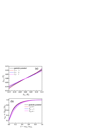
Figure 6: (Color online) (a) The hole ground state splitting, calculated for $\beta=0.15$, as a function of parameter $\Delta_{\text{cr}}/E_{0}$ for parabolic and Gaussian potential with $\tilde{V}_{\text{off}}=8;2;1$; (b) The dimensionless function $v_{\text{int}}(\beta)$ as the function of the light-hole to heavy-hole effective mass ratio $\beta$. Solid lines - results of numerical calculations, dotted lines - perturbation theory with the use of the trial functions.

The dependencies of the hole ground state splitting $\Delta_{\text{int}}$ on $\Delta_{\text{cr}}$, calculated numerically for the holes confined in parabolic and Gaussian potentials are shown on Fig. 6 (a) for $\beta=0.15$. It is clear that for small values of $\Delta_{\text{cr}}$ corresponding curves can be linearised, and the effect of the crystal field can be considered as perturbation EfrosPRB92 ; EfrosPRB96 :

$$\Delta_{\rm int}=\Delta_{\rm cr}v_{\rm int}=\Delta_{\rm cr}\int drr^{2}[R_{0}^{2}(r)-(3/5)R_{2}^{2}(r)]\,.$$ (31)

The function $v_{\rm int}$ depends on the ratio $\beta$ and, generally, may depend on the form of the QD potential. The dependencies of $v_{\rm int}(\beta)$ for parabolic potential and Gaussian potential with $\tilde{V}_{\text{off}}=8;2;1$ calculated numerically and obtained by using Eq. (31) with the trial function $R_{0}$ and $R_{2}$ in the form (26) are shown in Fig. 6 (b). A good agreement between two methods can be seen. The function $v_{\rm int}(\beta)$ only slightly depends on the value of $\tilde{V}_{\text{off}}$, but the $|M|=3/2$ states always correspond to the ground hole state EfrosPRB92 ; EfrosPRB96 . The function $v_{\rm int}$ increases from 0.2 for $\beta=0$ to 1 for $\beta=1$. The value of $v_{\rm int}$ at $\beta=0$ is determined by Eq. (25) resulting in $\int R_{2}^{2}r^{2}dr=\int R_{0}^{2}r^{2}dr=1/2$. For $\beta=1$, $v_{\rm int}=1$ is explained by the vanishing of $R_{2}$.

IV.2.2 Effect of the shape anisotropy

Figure 7 (a) shows the dependencies of the anisotropy induced hole ground state splitting $\Delta E^{\rm a}$ calculated numerically for parabolic and Gaussian potentials on anisotropy parameter $\mu$. Figure shows that in rather wide range of $\mu$ these dependencies can be approximated as linear with a good accuracy. In this case the splitting can be also found by the perturbation theory in two ways. One way is to consider as the perturbation the correction to the potential energy, $V_{\rm p}$ introduced in Eq. (12) for parabolic and by Eq. (20) for the Gaussian potentials. For such a perturbation the hole energy splitting $\Delta E^{\rm a}=\Delta_{\rm p}^{\rm a}$ can be found asRodina2010

$$\Delta_{\rm p}^{\rm a}=\frac{4\mu}{15}\frac{\hbar^{2}}{m_{h}L^{4}}\int drr^{4}R_{0}(r)R_{2}(r)\,$$ (32)

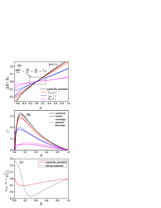
Figure 7: (Color online) (a) The dimensionless splitting of the hole ground state, calculated numerically, $\Delta E^{\rm a}/E_{0}$ (solid lines), and by two perturbation theory methods: $~{}\Delta_{\rm p}^{\rm a}/E_{0}$ (dotted lines), and $\Delta_{\rm k}^{\rm a}/E_{0}$ (dashed lines), calculated with numerically obtained functions $R_{0}(r)$ and $R_{2}(r)$ for parabolic and Gaussian QDs; (b) The coefficient of the linearisation, $C=\Delta E^{\rm a}/(E_{0}\mu)$, calculated numerically (solid curves) and using the trial functions via perturbation in kinetic (dotted curves) and potential (dashed curves) energy; (c) The relative energy splitting, $u_{sh}=-{\Delta E^{\rm a}}/{(2\mu E_{3/2}}=-{C}/{2\varepsilon_{3/2}}$, calculated for the parabolic (solid curve) and abrupt infinite potential (dashed curve).

In the second way one can use the change of coordinates Eq. (21) in order to obtain the perturbation correction to the hole kinetic energyEfrosPRB93 ; misprint :

$$\hat{H}^{\rm a}_{\rm k}=\frac{2\mu}{3}\frac{\hbar^{2}}{2m_{0}}[(\gamma_{1}+\frac{5}{2}\gamma)(\hat{k}^{2}-3\hat{k}_{z}^{2})-\\ -2\gamma[(\hat{\bm{k}}{\bm{j}})^{2}-3\{(\hat{\bm{k}}{\bm{j}}){\hat{k}_{z}}j_{z}\}]]\,,$$ (33)

where $\{ab\}=(ab+ba)/2$. Then the hole energy splitting $\Delta E^{\rm a}=\Delta_{\rm k}^{\rm a}$ can be found asEfrosPRB93

$$\Delta_{\rm k}^{\rm a}=\frac{\mu\hbar^{2}}{3m_{h}}\left[I_{1}^{\rm a}-\frac{1}{5}I_{2}^{\rm a}+\frac{4}{5}I_{3}^{\rm a}-\frac{1}{\beta}\left(I_{1}^{\rm a}-\frac{1}{5}I_{2}^{\rm a}-\frac{4}{5}I_{3}^{\rm a}\right)\right]\,,$$ (34)

where

$$I_{1}^{\rm a}=\int r^{2}dr\left[\frac{dR_{0}(r)}{dr}\right]^{2}\,,\\ ~{}I_{2}^{\rm a}=\int r^{2}dr\left(\left[\frac{dR_{2}(r)}{dr}\right]^{2}+\frac{6R_{2}(r)^{2}}{r^{2}}\right)\,,\\ I_{3}^{\rm a}=\int r^{2}drR_{2}(r)\left[\frac{d^{2}R_{0}(r)}{dr^{2}}-\frac{dR_{0}(r)}{rdr}\right]\,.$$ (35)

Calculations using radial wave functions $R_{0}$ and $R_{2}$ found by the numerical method results into $\Delta_{\rm p}^{\rm a}=\Delta_{\rm k}^{\rm a}=C\mu E_{0}$ with a good accuracy for small $\mu$ shown in Fig. 7 (a) and for all values of light to heavy holes effective mass ratio $\beta$. Figure 7 (b) shows the linear coefficients $C$ as functions of $\beta$. Dotted curves are calculated numerically, solid and dashed curves correspond to $C=\Delta_{\rm k}^{\rm a}/\mu/E_{0}$ and $C=\Delta_{\rm p}^{\rm a}/\mu/E_{0}$ calculated with the wave functions found via the variational procedure. Figure shows, that the accuracy of the variational method is rather good. Moreover, the kinetic energy and potential energy corrections found with the variational wave functions give the estimations of the value of $C$ from above and from below, respectively.

For the small values of $\mu$ linear corrections to the energy shift of the central of level position vanishes and $E_{1S_{3/2}}^{a}=(E_{1S_{3/2},~{}1/2}+E_{1S_{3/2},~{}3/2})/2\approx E_{1S_{3/2}}$. Numerical calculations show that for complex valence band the following approximation $E_{1S_{3/2}}^{a}\approx E_{1S_{3/2}}\left[1-\xi{\mu^{2}}/{9}\right]$ is valid, with factor $\xi$ being different from unity by no more than 10%. Parameter $\xi$ is the function of $\beta$ and $V_{\text{off}}$. Figure 7 (c) shows the relative to the quantum size energy splitting, $u_{sh}=-\frac{\Delta E^{\rm a}}{2\mu E_{3/2}}=-\frac{C}{2\varepsilon_{3/2}}$, introduced in EfrosPRB93, ; EfrosPRB96, (the sign ”-” is because of the opposite definition of the sign of anisotropy parameter $\mu$) and calculated for parabolic and abrupt potentials. One can see that there is the significant difference between the dependencies caused by the different shape of the QD potential. The shape anisotropy at the abrupt potential in general induces much larger relative splitting than that at the smooth one. Moreover, $u_{sh}$ changes sign for abrupt potential at $\beta\approx 0.15$, while remains always of the same sign in the smooth potential.

V Hole effective $g$-factor

In this section we consider the effect of external magnetic field on the holes states localized in quantum dots with the shape close to spherical. For this purpose we follow the conventional approachLuttinger ; Roth ; Gelmont73 ; EfrosPRB96 ; Rego97 ; Ivchenko ; BirPikus ; Kubisa11 ; Semina2015 and explore the hole representation of the Luttinger Hamiltonian with the external magnetic field ${\bm{B}}$ included in spherical approximation.Gelmont73 In a weak magnetic field, the top of the degenerated valence band is split according to the Zeeman term

$$\widehat{H}_{Z}=-2\mu_{B}\varkappa\left(\bm{j}\bm{B}\right).$$ (36)

Here $\mu_{B}$ – is the Bohr magneton, $\varkappa$ is the Luttinger magnetic parameter, and the lowest valence hole state has projection $j_{z}=3/2$ on the direction of magnetic field for the semiconductors with $\varkappa>0$.

The effect of a weak external magnetic field on the holes confined in some potential of the spherical symmetry can be considered as the perturbation. The resulting Zeeman splitting of the localized hole states is given by Gelmont73 ; EfrosPRB96 ; EfrosCh3 ; Semina2015

$$\widehat{H}_{\rm eff}=-\mu_{B}g_{\rm h}\left(\bm{J}\bm{B}\right).$$ (37)

Here $g_{\rm h}$ is the hole effective $g$-factor. For the hole ground state with $J=3/2$ its value can be determined via the radial wave functions $R_{0}$ and $R_{2}$ as:Gelmont73

$$g_{\rm h}=2\varkappa+\frac{8}{5}\gamma I_{1}^{\text{g}}+\frac{4}{5}\left[\gamma_{1}-2\left(\gamma+\varkappa\right)\right]I_{2}^{\text{g}}\,,$$ (38)

where

$$I_{1}^{\text{g}}=\int\limits_{0}^{\infty}r^{3}R_{2}(r)\frac{dR_{0}(r)}{dr}dr,~{}I_{2}^{\text{g}}=\int\limits_{0}^{\infty}r^{2}R_{2}^{2}(r)dr\,.$$ (39)

The integrals $I_{1}^{\text{g}}$ and $I_{2}^{\text{g}}$ describe the effect of the light- and heavy-hole mixing induced by the confining potential. Their values depend on the light- to heavy-hole effective mass ratio $\beta$ and do not depend on the QD size.EfrosPRB96 ; EfrosCh3 In the limit $\beta=1$ the holes mixing vanishes and $g_{\rm h}(\beta=1)=2\varkappa$. In the opposite case, $\beta\rightarrow 0$, the values of the mixing integrals can be found analytically as $I_{1}^{\text{g}}=-3/4$ and $I_{2}^{\text{g}}=1/2$ in any spherical symmetry potential using the differential condition Eq. (25). This results inGelmont73

$$g_{\rm h}(\beta=0)=\frac{6}{5}\varkappa+\frac{2}{5}\gamma_{1}-2\gamma\,.$$ (40)

Using the relation $\varkappa=-2/3+5\gamma/3-\gamma_{1}/3,$EfrosCh3 ; DKK we obtain from Eq. (40) that $g_{\rm h}(\beta=0)\approx-0.8$ corresponding to the lowest hole state with projection $M=-3/2$ on the magnetic field. Thus, in semiconductors with small values of $\beta$ the mixing of the valence subbands may result in different ordering of the Zeeman sublevels comparing with the free valence band edge states.

We examine further the effect of the valence band mixing on the hole effective $g$-factor in the QDs with different potential profiles. The dependencies of the mixing integrals $I_{1}^{\text{g}}$ and $I_{2}^{\text{g}}$ on $\beta$, calculated variationally (dotted lines) and numerically (solid lines) for the parabolic (black lines) and Gaussian with $\tilde{V}_{\text{off}}=1$, smooth potentials and infinite abrupt potential are shown on Fig. 8. In fact, the difference between values calculated variationally and numerically for smooth potentials is very small for any mass ratio and can be hardly seen on Figure, as well as the difference between values calculated for the parabolic and Gaussian smooth potential. This demonstrates the exceptional accuracy of the variational method. Moreover, $I_{1}^{\text{g}}$ and $I_{2}^{\text{g}}$ are practically independent of $\tilde{V}_{\text{off}}$ (as long as a confined level in Gaussian QD exists), while the hole wave functions are strongly dependent on $\tilde{V}_{\text{off}}$ (see, for example, Fig. 5 showing the resulting trial parameters). As a result, the $g$-factor for the hole in the parabolic and Gaussian QDs can be estimated with a good accuracy using the simple universal approximation of the $\beta$-dependence for mixing integrals:

$$I_{1}^{\text{g}}\approx e^{-5.145\beta}(1-\beta)\\ \left(-29.77\beta^{5}-37.97\beta^{3}+7.15\beta^{2}-7.77\beta-0.75\right),\\ I_{2}^{\text{g}}\approx 0.5e^{-7.35\beta^{1.127}}(1-\beta)\left(14.23\beta^{2.58}+1\right).$$ (41)

In contrast, Fig. 8 shows the noticeable difference between mixing integrals $I_{1}^{\text{g}}$ and $I_{2}^{\text{g}}$ calculated for smooth potentials, and for infinite abrupt potential. EfrosPRB96 It means that the magneto-optical properties of QDs with smooth and abrupt potentials can be quite different.

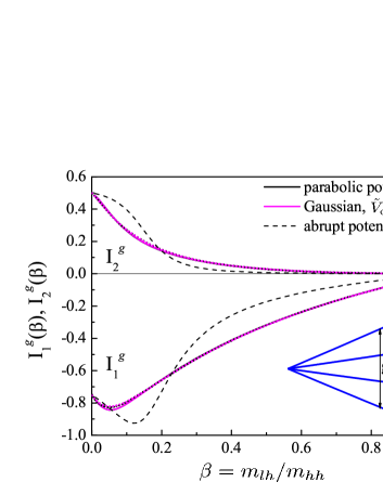
Figure 8: (Color online) Dimensionless integrals, $I_{1}^{\text{g}}$ and $I_{2}^{\text{g}}$, defining the hole ground state $g$-factor in spherical quantum dot, Eq. (38), with parabolic, Gaussian with $\tilde{V}_{\text{off}}=1$ and abrupt infinite potential EfrosPRB96 as a function of $\beta$. Solid lines correspond to variational calculation, dotted lines to numerical calculation, dashed lines correspond to the abrupt infinite potential.

In the spherically-symmetric QDs, the hole ground state in zero magnetic field is fourfold degenerate with respect to the momentum projection $M$. Hence, in agreement with Eq. 37 the ground state splits in weak magnetic fields into four equidistant sublevels (see the inset in Fig. 8). So, the two effective $g$-factors can be introduced in this case: $g_{1/2}=g_{\rm h}$ for the splitting of the states with momentum projection $M\pm 1/2$ on the magnetic field direction and $g_{3/2}=3g_{\rm h}$ for the states with momentum projection $M=\pm 3/2$. The lowest hole state is always $M=-3/2$ for semiconductors with $\beta\rightarrow 0$ and $M=+3/2$ ($M=-3/2$) for semiconductors with $\varkappa>0$ ($\varkappa<0$) and $\beta\rightarrow 1$.

In the axially symmetric QD the joint effect of the anisotropy and magnetic field depends on the direction of magnetic field with respect to the direction of the anisotropy axis $z$. In the case of small anisotropy, for ${\bm{B}}||z$ the hole effective $g$ factors for $M=\pm 3/2$ and $M=\pm 1/2$ states remain the same: $g_{3/2}=3g_{\rm h}$ and $g_{1/2}=g_{\rm h}$, respectively. Semina2015 For the ${\bm{B}}\perp z$ they become strongly anisotropic: the linear on ${\bm{B}}$ splitting of $\pm 3/2$ states vanishes, whereas the splitting of $\pm 1/2$ states is described by the effective $g$ factor equal to $g_{1/2}^{\perp}=2g_{\rm h}$. Such consideration is valid while the magnetic field induced splitting is smaller than the zero field energy splitting $\Delta E^{\rm a}$. In addition, the ${\bm{B}}\perp z$ mixes the hole states with $M=\pm 3/2$ and $M=\pm 1/2$.EfrosPRB96 ; EfrosCh3

In the case of highly anisotropic QDs, i.e. in the limit of the quantum disk or quantum wire, it can be convenient to describe the hole states in the framework of Luttinger spinors introduced in Ref. Rego97, and classify the hole states by parity quantum number and $z$-component of the total angular momentum, which determine their splitting in the magnetic field. In these cases, the hole $g$-factors are substantially different from the values of $g_{3/2}$ and $g_{1/2}$, calculated above. The respective anisotropic $g$-factor values were calculated in Ref. Semina2015, for the model of the parabolic potential.

VI Discussion

In this paper we presented the detailed study of the hole states in quantum dots with the smooth potential shape of rotational symmetry, which can be realized in II-VI structures. We developed the variational approach with only three trial parameters, which allowed us to calculate with a good accuracy not only the hole energy but also its $g$-factor and energy splitting of ground state caused by an anisotropy of the quantum dot shape or the crystal field. These quantities occur to be strongly dependent on the wave function and, therefore, very sensitive to the choice of the trial function. For example, we have found, that the simplified trial functions with the only trial parameter from Ref. Rodina2010, predict the hole ground state energy with a good accuracy, however do not allow to calculate the hole $g$-factor and anisotropy–induced splittings. The accuracy of the new trial functions and the developed variational method are verified by comparing the obtained results with numerical calculations. The advantage of the variational method is to allow one to have the hole envelope wave function in the simple analytical form that can be rather easily used for further modelling, e. g., of the multiexciton states in the QDs. At the same time, the developed numerical method allowed us to calculate the whole energy spectrum including the excited states of the holes in the smooth Gaussian–like potential. To the best of our knowledge, neither variational method nor numerical calculations (including the atomistic approaches) for the hole states in QDs with such a potential profile had not been reported before.

The general dependencies of the hole ground state characteristics (energy and localization radius) on QD potential depth and light to heavy hole effective mass ratio are calculated for spherical QDs. The effect of the QD anisotropy (potential shape or internal crystal field) on the hole ground state is considered. The general dependencies of the hole ground state splitting on potential depth and light to heavy hole effective mass ratio are obtained. In addition, the Zeeman splitting of the hole ground state due to the external magnetic field is studied. It is shown that the dependence of the hole effective $g$-factor on the depth of the QD potential is negligible and its dependence on $\beta$ for the QDs with the close to spherical shape can be well approximated by the universal analytical expressions. Moreover, the results obtained in Ref. Semina2015, for the hole effective $g$-factors in QDs modelled by the ellipsoidal parabolic potential profiles of arbitrarily anisotropy can be used for the case of the Gaussian-shaped QDs as well. Thus, in the limit of weak magnetic fields the effective hole $g$-factor is determined solely by the potential profile type, but does not depend on it’s size and barrier height. These results are in line with known independence of the effective $g$-factor of the localization energy of the hole bound to a deep or Coulomb–like acceptor centerGelmont73 ; Malyshev ; Malyshev2 and of the QD size.EfrosPRB96 ; EfrosCh3 In contrast, the Zeeman splittings and the zero field splittings caused by the QD shape anisotropy are quite different for the abrupt and the smooth confining potentials. Such a difference may include even different ordering of the hole states both in zero and in external magnetic field. Therefore, the combining of the smooth and abrupt potentials, e.g. by variation of QD composition, opens new possibilities to designing the structures with the needed properties of the hole states.

Let us discuss the applicability of the developed model to the II-VI QDs with gradually varying concentration. Peranio2000 ; Litvinov2008 ; Nasilowski15 The potential profile in such dots indeed can be approximated by the Gaussian. However, the varying of concentration implies also the spatial variation of the effective mass parameters. In II-VI QDs the variation of the effective mass parameters is not large and for the first approximation the mean values can be used with our model. The energy corrections caused by the effective mass spatial variation are expected to be of the same order of magnitude as the corrections caused by the non-parabolicity of the energy dispersion (terms $\propto\hat{k}^{4}$).Volkov99 Therefore, they should be considered in the framework of the Kane ${\bm{k}}{\bm{p}}$ model taking into account the interaction between conduction and valence bands and that may be a subject of a future study.

VII acknowledgments

The authors are thankful to T.V. Shubina and R.A. Suris for stimulating discussions. The work was supported by Russian Science Foundation (Project number 14-22-00107).

References

- (1) S.V. Ivanov, S.V. Sorokin, I.V. Sedova, ”Molecular beam epitaxy of wide-gap II-VI laser heterostructures” in Molecular Beam Epitaxy, 611-630 (Elsevier, 2013).
- (2) S.V. Sorokin, S.V. Gronin, I.V. Sedova, M.V. Rakhlin, M.V. Baidakova, P.S. Kop‘ev, A.G. Vainilovich, E.V. Lutsenko, G.P. Yablonskii, N.A. Gamov, E.V. Zhdanova, M.M. Zverev, S. S. Ruvimov, S.V. Ivanov, Semiconductors 49, 331 (2015).
- (3) S. Strauf, S. M. Ulrich, K. Sebald, P. Michler, T. Passow, D. Hommel, G. Bacher, and A. Forchel, Phys. Stat. Sol. (b) 238, 321 (2003).
- (4) A. Tribu, G. Sallen, T. Aichele, R. André, J.-P. Poizat, C. Bougerol, S. Tatarenko, and K. Kheng, Nano Lett. 8 (12), 4326 (2008).
- (5) O. Fedorych, C. Kruse, A. Ruban, D. Hommel, G. Bacher, and T. Kümmell. Appl. Phys. Lett. 100, 061114 (2012).
- (6) A. Klochikhin, A. Reznitsky, B. D. Don, H. Priller, H. Kalt, C. Klingshirn, S. Permogorov, and S. Ivanov, Phys. Rev. B 69, 085308 (2004).
- (7) N. Peranio, A. Rosenauer, D. Gerthsen, S. V. Sorokin, I. V. Sedova, and S. V. Ivanov, Phys. Rev. B 61, 16015 (2000).
- (8) D. Litvinov, M. Schowalter, A. Rosenauer, B. Daniel, J. Fallert, W. Löffler, H. Kalt, and M. Hetterich, Phys. Stat. Sol. (a) 205, 2892 (2008).
- (9) V. D. Kulakovskii, G. Bacher, R. Weigand, T. Kümmell, A. Forchel, E. Borovitskaya, K. Leonardi and D. Hommel, Phys. Rev. Lett. 82, 1780 (1999).
- (10) M. Syperek, D. R. Yakovlev, I. A. Yugova, J. Misiewicz, I. V. Sedova, S. V. Sorokin, A. A. Toropov, S. V. Ivanov, and M. Bayer, Phys. Rev. B 84, 085304 (2011).
- (11) A. Reznitsky, M. Eremenko, I. V. Sedova, S. V. Sorokin and S. V. Ivanov, Phys. Status Solidi B, 1-8 (2015).
- (12) M. Nasilowski, P. Spinicelli, G. Patriarche, and B. Dubertret, Nano Lett. 15 (6), 3953 (2015).
- (13) G.E. Cragg, and Al.L. Efros, Nano Letters 10, 313 (2010).
- (14) F. Garcia-Santamaria, S. Brovelli, R. Viswanatha, J.A. Hollingsworth, H. Htoon, S.A. Crooker, and V.I. Klimov, Nano Letters 11, 687 (2011).
- (15) W. K. Bae, L. A. Padilha, Y.-S. Park, H. McDaniel, I. Robel, J. M. Pietryga, and V. I. Klimov, ACS Nano, 7 (4), 3411 (2003).
- (16) J.I. Climente, J.L. Movilla, and J. Planelles, Small 8 (5), 754 (2012).
- (17) M. Korkusinski, O. Voznyy, and P. Hawrylak, Phys. Rev. B 82, 245304 (2010).
- (18) M. Zielinski, Y. Don, and D. Gershoni, Phys. Rev. B 91, 085403 (2015).
- (19) R. Singh and G. Bester, Phys. Rev. Lett. 104, 196803 (2010).
- (20) Al. L. Efros and A. L. Efros, Sov. Phys. Semicond. 16, 772 (1982).
- (21) L. E. Brus, J. Chem. Phys. 80, 4403 (1984).
- (22) J. L. Marin, R. Rier and S. A. Cruz, J. Phys.: Condens. Matter 10, 1349 (1998).
- (23) G. Pellegrini, G. Mattei, P. Mazzoldi, Journal of Applied Physics 97(7), 073706 (2005).
- (24) D. Schooss, A. Mews, A.Eychmuller, and H. Weller, Phys. Rev. B 49, 17072 (1994).
- (25) L. G. C. Rego, P. Hawrylak, J. A. Brum, and A. Wojs, Phys. Rev. B 55, 15694 (1997).
- (26) Xie Wen-Fang, Physica B: Physics of Condensed Matter 358, 109 (2005).
- (27) W. Que, Phys. Rev. B 45, 11036 (1992).
- (28) J. Adamowski, M. Sobkowicz, B. Szafran, and S. Bednarek, Phys. Rev. B 62, 4234 (2000).
- (29) M. Ciurla, J. Adamowski, B. Szafran, S. Bednarek, Physica E 15, 261 (2002).
- (30) Xie Wen-Fang, Superlattices and Microstructures 46 693 (2009).
- (31) B. Szafran, S. Bednarek, and J. Adamowski, Phys. Rev. B 64, 125301 (2001).
- (32) A. Wojs, P. Hawrylak, S. Fafard, L. Jacak, Phys. Rev. B 54, 5604 (1996).
- (33) J.M. Luttinger, Phys. Rev. 102, 1030 (1956).
- (34) M. Kubisa, K. Ryczko, and J. Misiewicz, Phys. Rev. B 83, 195324 (2011).
- (35) M.A. Semina, R.A. Suris, Semiconductors 49 (6), 797 (2015).
- (36) Al. L. Efros and A. V. Rodina, Solid State Commun. 72, 645 (1989).
- (37) J.B. Xia, Phys. Rev. B 40, 8500 (1989).
- (38) A. I. Ekimov, F. Hache, M.C. Schanne-Klein, D. Ricard, C. Flytzanis, I. A. Kudryavtsev, T. V. Yazeva, A.V. Rodina, and Al. L. Efros, J. Opt. Soc. Am. B 10, 100 (1993).
- (39) Al. L. Efros, M. Rosen, M. Kuno, M. Nirmal, D. J. Norris, and M. Bawendi, Phys. Rev. B 54, 4843 (1996).
- (40) Al. L. Efros and M. Rosen, Phys. Rev. B 58, 7120 (1998).
- (41) W. Jaskolski and G. W. Bryant, Phys. B 57, R4237 (1998).
- (42) C. Pryor, Phys. Rev. B 57, 7190 (1998).
- (43) O. Stier, M. Grundmann, and D. Bimberg, Phys. Rev. B 59, 5688 (1999).
- (44) M. Tadic, F. M. Peeters, and K. L. Janssens, Phys. Rev. B 65, 165333 (2002).
- (45) R. Rinaldi, P. V. Giugno, and R. Cingolani, H. Lipsanen, M. Sopanen, and J. Tulkki, J. Ahopelto, Phys. Rev. Lett 77, 342 (1996).
- (46) M.Korkusinski, P. Hawrylak, Phys. Rev. B 87, 115310 (2013).
- (47) A. Klochikhin, A. Reznitsky, Don,B.D., H. Zhao, H. Priller, H. Kalt, C. Klingshirn, D. Litvinov, D. Gerthsen, S. Permogorov, I. Sedova, S. Sorokin, S. Ivanov, in 10th International Symposium on Nanostructures: Physics and Technology, Proc. SPIE 5023, 546-549 (2002).
- (48) M. Abramowitz, I. Stegun, Handbook of Mathematical Functions with Formulas, Graphs, and Mathematical Tables, New York: Dover, p. 773, ISBN 978-0486612720, MR 0167642, (1965).
- (49) A. R. Edmonds, Angular momentum in Quantum mechanics, Princenton University Press, 1957.
- (50) B. L. Gel’mont and M. I. D’yakonov, Fiz. Techn. Polupr. 5, 2191 (1971).
- (51) Note, that the factor introduced because we use the definition of spherical harmonics as given in Ref. Edmonds, while in Ref. Gelmont71, the spherical harmonics were defined according to Ref. LL, .
- (52) N.O. Lipari and A. Baldereschi, Phys. Rev. Lett. 25, 1660 (1970).
- (53) A. Baldereschi and N.O. Lipari, Phys. Rev. B 8, 2697 (1973).
- (54) A.V. Rodina and Al. L. Efros, Phys. Rev. B 82, 125324 (2010).
- (55) L.D. Landau and E.M. Lifshitz, Quantum Theory, 2nd ed. (Pergamon, Oxford, 1965).
- (56) E. L. Ivchenko, Optical Spectroscopy of Semiconductor Nannostructures Springer, 2007.
- (57) G.L. Bir and G.E. Pikus, Symmetry and Strain-Induced Effects in SEmiconductors (Wiley, New York, 1974).
- (58) Al. L. Efros, Phys. Rev. B 46, 7448 (1992).
- (59) Al. L. Efros and A.V. Rodina, Phys. Rev. B 47, R10005 (1993).
- (60) There is the misprint in Ref. EfrosPRB93, : in Eq. (8) should be replaced by .Rodina2010
- (61) L. Roth, B. Lax, and S. Zwerdling, Rhys. Rev. 114, 90 (1959).
- (62) B. L. Gel’mont and M. I. D’yakonov, Fiz. Techn. Poluprov. 7, 2013 (1973).
- (63) Al. L. Efros, in Semiconductor and Metal Nanocrystals: Synthesis and Electronic and Optical Properties, edited by V. I. Klimov (New York : Marcel Dekker, Inc., 2004).
- (64) G. Dresselhaus, A. F. Kip, and C. Kittel, Phys. Rev. 98, 368 (1955).
- (65) A.V. Malyshev and I.A. Merkulov, Phys. Sol. State 39, 49 (1997) [Fiz. Tverd. Tela 39, 58 (1997)].
- (66) A.V. Malyshev, I.A. Merkulov, and A.V. Rodina, Phys. Stat. Sol. (b) 210, 1 (1998).
- (67) E. E. Takhtamirov, and V. A. Volkov, JETP 116, 1843. (1999).