Accelerated graph-based nonlinear denoising filters

Abstract

Denoising filters, such as bilateral, guided, and total variation filters, applied to images on general graphs may require repeated application if noise is not small enough. We formulate two acceleration techniques of the resulted iterations: conjugate gradient method and Nesterov’s acceleration. We numerically show efficiency of the accelerated nonlinear filters for image denoising and demonstrate 2-12 times speed-up, i.e., the acceleration techniques reduce the number of iterations required to reach a given peak signal-to-noise ratio (PSNR) by the above indicated factor of 2-12.

0.1 Introduction

Modern image denoising algorithms are edge preserving, i.e., they preserve important discontinuities in an image while attenuating noise. Many of such algorithms are based on the anisotropic diffusion idea, first formulated in [1, 2]. The idea consists in using diffusion coefficients depending on the local variance—the larger the variance the smaller the coefficient.

Popular denoising techniques, which implement the anisotropic diffusion, include the bilateral filter [3, 4, 5, 6, 7], the guided image filter [10], and the total variation denoising [11]. The fastest computer implementations of the bilateral filter are proposed in recent papers [8, 9]. The guided image filter has been included in the MATLAB Image Processing Toolbox. We also remark that the total variation denoising can be formulated in the filter form; see Section 0.2.3. All the three filters may be applied to images or signals on graphs; see, e.g., [12] on the graph-based methods in signal and image processing.

More recent state-of-the-art denoising methods are patch-based such as those developed in [13, 14, 15, 16, 17]. An improvement of these methods, based on a special truncation of high frequency modes, is proposed in [18, 19]. Since the patch-based algorithms use geometrically similar patches, they seem to be inconvenient for images or signals on general graphs. This reason might partially justify a still active research interest in the basic imaging techniques like the bilateral filter, guided image filter and total variation denoising. Moreover, the models based on the total variation enjoy very rich variational properties.

In certain situations, a single application of a smoothing filter does not produce an acceptable denoising result, and, therefore, the filter transform has to be applied repeatedly (or iteratively), say 10-1000 times, depending on the filter type and level of noise. The repetitive application procedure may be expensive even for images of moderate size. Our previous work in [22, 23] is devoted to acceleration techniques for the iterative application of smoothing filters formulated above. The results are based on the studies in [20, 21], where low-pass filters are constructed by means of projection onto the leading invariant subspaces, corresponding to the modes of lowest frequency, of a graph Laplacian matrix generated by a basic smoothing filter.

The initial publications [20, 21, 22] consider iterative application of a fixed smoothing filter, whose coefficients are defined by the input noisy image. Such a method is known under the name of power iteration. The authors of [20] propose to accelerate the power iteration by the aid of Chebyshev’s polynomials. The paper [21] additionally proposes to accelerate the power iteration by the aid of the polynomials generated in the conjugate gradient method [25]. In [22], we formulate a special variant of the preconditioned conjugate method, which accelerates the power iteration for 1D and 2D signals on graphs, and demonstrate that similar acceleration can be achieved with the LOBPCG method [26].

The subsequent works [23, 24] deal with a nonlinear iterative application of filters, where a smoothing filter at each iteration is determined by the currently processed image. The resulting transform yields a nonlinear smoothing filter in contrast to the linear smoothing filter given by the power iteration with a fixed filter at each iteration. The paper [23] presents a special variant of a nonlinear preconditioned conjugate gradient method and numerically demonstrates its high efficiency for accelerated denoising of one-dimensional signals. The conference presentation [24] shows how to accelerate the nonlinear iterative filters by means of the Chebyshev polynomials.

The present note continues the work in our previous papers [22, 23] about acceleration of iterative smoothing filters and contains a number of new contributions listed below. In addition to the bilateral and guided image filters, we consider the total variation denoising and formulate it as a filter operator. In addition to the preconditioned conjugate gradient (PCG) acceleration of nonlinear iterative smoothing filters, we propose to apply Nesterov’s acceleration, which is commonly used in a totally different context of iterative solution of convex minimization problems. We numerically investigate performance of the PCG acceleration of nonlinear iterative smoothing filters for two-dimensional images, which is not clear from the previous publications at all. We also numerically investigate performance of Nesterov’s acceleration of nonlinear iterative smoothing filters.

0.2 Smoothing filters

We consider only smoothing filters, which are represented in the matrix form $x^{1}=D^{-1}Wx^{0}$, where the vectors $x^{0}$ and $x^{1}$ of length $N$ are the input and output signals, respectively. The entries $w_{ij}$ of the symmetric $N\times N$ matrix $W$ are determined by a guidance signal $g$, i.e. $W=W(g)$. When $g=x^{0}$, the filter is nonlinear and called self-guided. The diagonal matrix $D$ has $N$ positive diagonal entries $d_{i}=\sum_{j=1}^{N}w_{ij}$. The symmetric nonnegative definite matrix $L=D-W$ is commonly referred to as a graph Laplacian matrix. The spectrum of the normalized Laplacian $D^{-1/2}LD^{-1/2}$ is nonnegative real, and its largest eigenvalues correspond to the highest oscillation modes.

In this paper, we are interested in iterative application of the filter transform

$$x^{k+1}=D^{-1}Wx^{k},\qquad k=1,\dots,k_{\max},$$

where the number of iterations $k_{\max}$ needs to be chosen large enough for good denoising result in $x^{k_{\max}}$, but small enough to prevent over-smoothing effect. Each iteration $k$ is a self-guiding filter, where the weights $w_{ij}$ are determined by the guidance signal $g=x^{k}$.

0.2.1 Bilateral filter (BF)

Let us assume that a spatial distance $\|p_{i}-p_{j}\|\in[0,\infty]$ can be defined for all index pairs $(i,j)$, $1\leq i,j\leq N$. The weights of the bilateral filter [5] equal

$$w_{ij}=\exp\left(-\frac{\|p_{i}-p_{j}\|^{2}}{2\sigma_{d}^{2}}\right)\exp\left(-\frac{|g_{i}-g_{j}|^{2}}{2\sigma_{r}^{2}}\right),$$

where the constants $\sigma_{d}$ and $\sigma_{r}$ are filter parameters, and $|g_{i}-g_{j}|$ is a suitable distance between the components of a guidance signal $g$. The arithmetical complexity of a single application of the bilateral filter to images on rectangular grids can be reduced to $O(N)$; see [8].

0.2.2 Guided filter (GF)

The following algorithm, proposed in [10] and implemented in the MATLAB Image Processing Toolbox, performs one application of the guided filter defined by a guidance signal $g$:

Algorithm Guided filter
Input: $x$, $g$, $w$, $\epsilon$
Output: $y$
$mean_{g}=f_{mean}(g,w)$; $mean_{x}=f_{mean}(x,w)$
$corr_{g}=f_{mean}(g.*g,w)$; $corr_{gx}=f_{mean}(g.*x,w)$
$var_{g}=corr_{g}-mean_{g}.*mean_{g}$; $cov_{gx}=corr_{gx}-mean_{g}.*mean_{x}$
$a=cov_{gx}./(var_{g}+\epsilon)$; $b=mean_{x}-a.*mean_{g}$
$mean_{a}=f_{mean}(a,w)$; $mean_{b}=f_{mean}(b,w)$
$y=mean_{a}.*g+mean_{b}$

The function $f_{mean}(\cdot,w)$ denotes a mean filter with the window width $w$. The positive constant $\epsilon$ determines the smoothness degree—the larger $\epsilon$ the larger smoothing effect. The dot preceded operations $.*$ and $./$ denote the componentwise multiplication and division of vectors or matrices. Special implementations of the guided filter applied to images on rectangular grids achieve an $O(N)$ arithmetical complexity; see [10].

The above algorithm does not explicitly build the matrices $W$ and $D$ for the filter transform $y=D^{-1}Wx$. Nevertheless, the transform is linear, and its matrix coincides with $W$, when boundary padding for the mean filter $f_{mean}(\cdot,w)$ is defined carefully so that the matrix $W(g)$ would be symmetric. Thus, the diagonal matrix $D$ for the guided filter equals the identity matrix $I$ [10], and the graph Laplacian matrix is $L=I-W$.

0.2.3 Total Variation filter (TVF)

Let $\nabla$ denote a gradient operator acting on signals. The classical Rudin-Osher-Fatemi (ROF) denoising model [11] reads as follows:

$$\min_{x}\|\nabla x\|_{1}\mbox{ subject to }\|x-x^{0}\|_{2}=\sigma,$$

where $\sigma>0$ is given. Solution of ROF for a two-dimensional continuous image $x^{0}(x,y)$ is approximated by the solution $u(x,y,t)$ of the following boundary value problem for sufficiently large $t>0$, a suitable constant $\lambda>0$, and sufficiently small regularizing parameter $\epsilon>0$:

$$u_{t}=\frac{\partial}{\partial x}\left(\frac{u_{x}}{\sqrt{u_{x}^{2}+u_{y}^{2}}+\epsilon}\right)+\frac{\partial}{\partial y}\left(\frac{u_{y}}{\sqrt{u_{x}^{2}+u_{y}^{2}}+\epsilon}\right)-\lambda(u-x^{0})$$

$$u(x,y,0)=x^{0}(x,y);\quad\frac{\partial u}{\partial n}=0\text{ on the image boundary}.$$

The value $\|\nabla u\|_{1}=\iint\sqrt{u_{x}^{2}+u_{y}^{2}}dxdy$ is called the total variation of $u(x,y)$.

The graph Laplacian matrix associated with the ROF model is a suitable discretization of the elliptic operator $-\frac{\partial}{\partial x}\left(\frac{u_{x}}{\sqrt{u_{x}^{2}+u_{y}^{2}}+\epsilon}\right)-\frac{\partial}{\partial y}\left(\frac{u_{y}}{\sqrt{u_{x}^{2}+u_{y}^{2}}+\epsilon}\right)$ with the Neumann boundary conditions.

For a one-dimensional $N\times 1$ array $x$, we can, e.g., define the gradient operator $\nabla x=Gx$ by means of the bidiagonal $N\times N$ matrix

$$G=\begin{bmatrix}-1&1\\ &\ddots&\ddots\\ &&-1&1\\ &&&0\end{bmatrix}.$$

Given a one-dimensional guidance signal $g$ and regularization parameter $\epsilon>0$, we introduce a diagonal diffusion $N\times N$ matrix $\mbox{diag}(C)$ with the diagonal $C=\frac{1}{4}\left[\epsilon./(\epsilon+|\nabla g|)\right]$. The TV filter $y=D^{-1}Wx$ is then defined by the $N\times N$ matrices $L(g)=\nabla^{T}\mbox{diag}(C)\nabla=G^{T}\mbox{diag}(C)G$, $D(g)=I$, $W(g)=D-L$.

The gradient operator applied to a two-dimensional $M\times M$ array $x$ can be defined by the formula $\nabla x=\begin{bmatrix}p_{1}\\ p_{2}\end{bmatrix}=\begin{bmatrix}Gx\\ xG^{T}\end{bmatrix}$ with the bidiagonal $M\times M$ matrix $G$. The transposed gradient is the operator $\nabla^{T}\begin{bmatrix}p_{1}\\ p_{2}\end{bmatrix}=G^{T}p_{1}+p_{2}G$. For an $M\times M$ guidance array $g$, we use the coefficient matrix

$$C=\frac{1}{8}\left[\epsilon./\left(\epsilon+\sqrt{|Gg|.*|Gg|+|gG^{T}|.*|gG^{T}|}\right)\right],$$

which is rotation invariant. Then the Laplacian operator is $L(g)x=\nabla^{T}\left(\begin{bmatrix}C\\ C\end{bmatrix}.*\nabla x\right)=G^{T}(C.*Gx)+(xG^{T}.*C)G$, $D(g)=I$, and $W(g)=D-L$.

In the case of general graph-based signal $x$ and guidance $g$, one can use the above formulas for the one-dimensional case with a problem specific gradient operator.

0.3 Acceleration of iterations

In this section, we provide two algorithms for acceleration of the non-linear filtering iteration $x_{0}=x$, $x_{k+1}=D^{-1}(x_{k})W(x_{k})x_{k}=x_{k}-D^{-1}(x_{k})L(x_{k})x_{k}$, $k=0,1,\ldots,k_{\max}$, where the symmetric matrices $W(g)$ and $D(g)$ are defined in Section 0.2, and $L(g)=D(g)-W(g)$. In both algorithms, the total running time is determined by the number of calls to the basic filter $x_{k+1}=D^{-1}(x_{k})W(x_{k})x_{k}$. The overhead due to the auxiliary computations for the accelerations is marginal with respect to the application of the basic filters to images on general graphs.

0.3.1 Acceleration by the Preconditioned Conjugate Gradient (PCG) method

Formally applying the classical preconditioned conjugate gradient method [25] with a preconditioner $D$ to the system of linear equations $Lu=0$, and choosing $D$ and $W$ depending on the current approximation $y$ to the solution, we arrive at the following algorithm, proposed and partially tested in [21, 22, 23]. We draw attention to the necessity of restarts in the algorithm due to the nonlinearity of power iterations. We also emphasize that convergence theory of PCG in the considered context does not exist.

Algorithm PCG($k_{\max}$) with $l_{\max}$ restarts
Input: $x$, $k_{\max}$, $l_{max}$
Output: $y$
$y=x$
for $l=1,\ldots,l_{\max}$ do
$r=W(y)y-D(y)y$
for $k=1,\ldots,k_{\max}-1$ do
$s=D^{-1}(y)r$
$\gamma=s^{T}r$
if $k=1$ then $p=s$
else $\beta=\gamma/\gamma_{old}$; $p=s+\beta p$
endif
$q=D(y)p-W(y)p$
$\alpha=\gamma/(p^{T}q)$
$y=y+\alpha p$
$r=r-\alpha q$
$\gamma_{old}=\gamma$
endfor
endfor

0.3.2 Nesterov’s acceleration

Nesterov’s acceleration is suggested in [28]. The choice of $\beta$ in the following algorithm has been adopted from [29]. To our best knowledge, convergence theory of Nesterov’s acceleration in the present context is not available.

Algorithm Nesterov($k_{\max}$)

Input: $x$, $k_{\max}$

Output: $y$

$y=x$; $y_{old}=y$

for $k=1,\ldots,k_{\max}$ do

$\beta=(k-1)/(k+2)$

$t=y+\beta(y-y_{old})$

$y_{old}=y$

$y=D^{-1}(t)W(t)t$

endfor

0.4 Numerical study

From the mathematical point of view, application of the smoothing filter transform $x^{1}=D^{-1}Wx^{0}$ to images on general graphs does not differ from the case of images on rectangular grids, if specific geometric properties of the rectangular grid on the plane are not taken into account. Therefore, in order to facilitate programming efforts in our numerical tests, we carry out numerical experiments with images on standard rectangular grids instead of images on general graphs. We use a gray-scale $512\times 512$-image created by the MATLAB command clean = phantom(’Modified Shepp-Logan’,512). The image is piecewise constant, and its intensity levels span the range $[0,1]$. A noisy image, generated by the MATLAB command noisy = imnoise(clean), is corrupted by Gaussian white noise with zero mean and variance equal to $0.01$. The peak signal-to-noise ratio (PSNR) of the noisy image is $21.7$. In order to show smaller details, we display the zoomed image patches consisting of the rows 211:420 and columns 201:300 instead of full $512\times 512$-images. But the filters are applied to full images, and the reported PSNR values are also computed for full images.

Our simple implementation of the bilateral filter has the the following parameters: the window width equals 5, $\sigma_{d}=1$, and $\sigma_{r}=0.2$. As the guided image filter, we use the function imguidedfilter from MATLAB with the window width 5 and the smoothness parameter $\epsilon=0.0001$. The regularization parameter in our implementation of the total variation filter equals $\epsilon=0.001$. The restart parameter in the preconditioned conjugate gradient acceleration is $k_{\max}=3$. According to our experience, the PCG acceleration of self-guided smoothing filters with $k_{\max}>5$ does not work well. We count the total number of iterations in the iterative filters as the number of calls of a basic filter. Therefore, the number of iterations in the PCG method equals $k_{\max}\times l_{\max}$.

Figure 2 displays zooms of the clean and noisy images. Figure 2 shows the denoising result of a single application of the guided image filter with the default MATLAB’s value of the smoothness parameter $\epsilon=0.01$. The image on the left has been processed with the window width 5, which is the MATLAB’s default value. The image on the right has been processed with the window width 30.

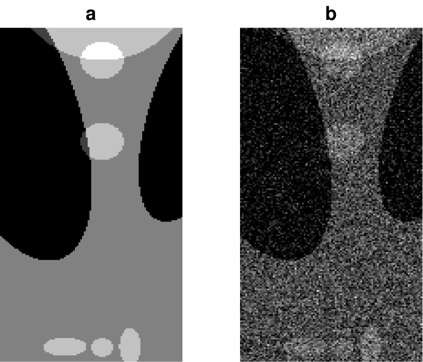
Figure 1: Clean image vs. noisy image, PSNR = $21.72$

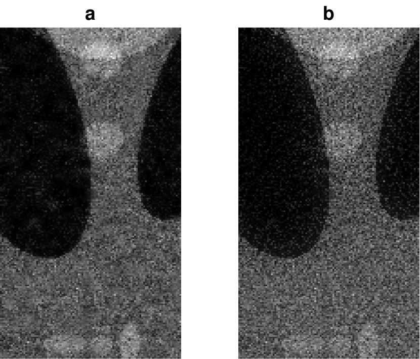
Figure 2: A single application of the guided filter with $\epsilon=0.01$. (a) window width $5$, PSNR=26.16 vs. (b) window width $30$, PSNR=24.84

Figures 3–5 illustrate the repeated application, the PCG accelerated iteration, and the Nesterov accelerated iteration, of the guided filter, the bilateral filter, and the total variation filter, respectively. We have chosen the filter parameters and number of iterations in order to reach sufficiently good visual quality of output images. We remark that selection of output results with the highest possible PSNR values is not always the best strategy for achieving the best visual quality.

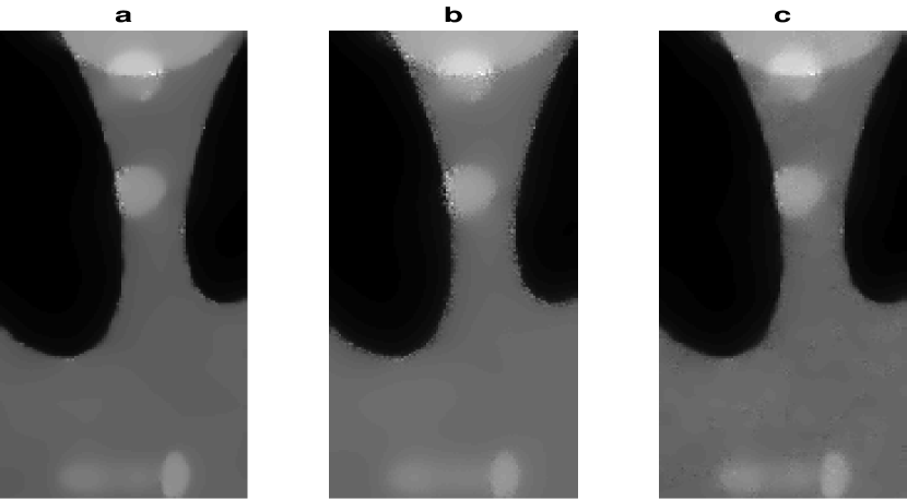
Figure 3: (a) 70 iterations of the repeated guided filter, PSNR=29.13, (b) 30 iterations of the PCG accelerated guided filter, PSNR=28.76,
(c) 23 iterations of the Nesterov accelerated guided filter, PSNR=29.01

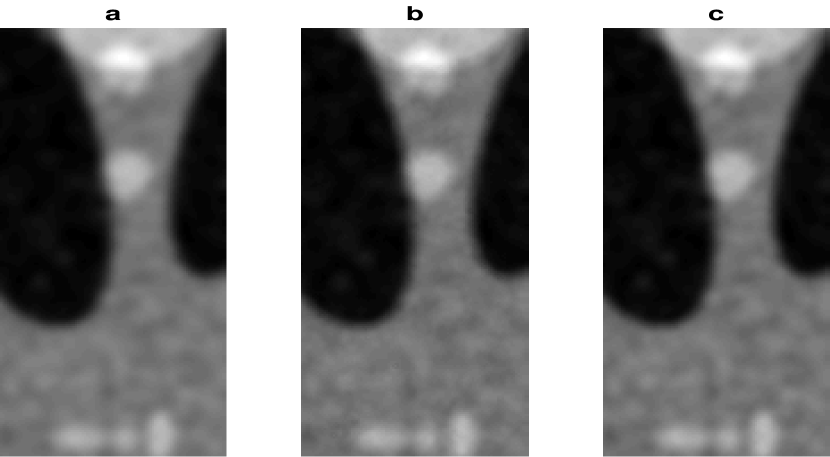
Figure 4: (a) 10 iterations of the repeated bilateral filter, PSNR=29.69, (b) 6 iterations of the PCG accelerated bilateral filter, PSNR=29.82, (c) 5 iterations of the Nesterov accelerated bilateral filter, PSNR=29.85

The results in Figures 3 and 4 show 2-3x speedup for the accelerated guided image and bilateral filters. The speedup for the accelerated total variation filter shown in Figure 5 is 8-12x. The visual quality of the images 5(a) and 5(b) is slightly better than that of 5(c). As concerns comparison of the two acceleration techniques by the preconditioned conjugate gradient method and by Nesterov’s acceleration, both methods usually possess similar speedup and output quality. However, sometimes Nesterov’s method behaves stabler in the acceleration of nonlinear iterations. The PCG acceleration is more efficient for acceleration of linear iterations.

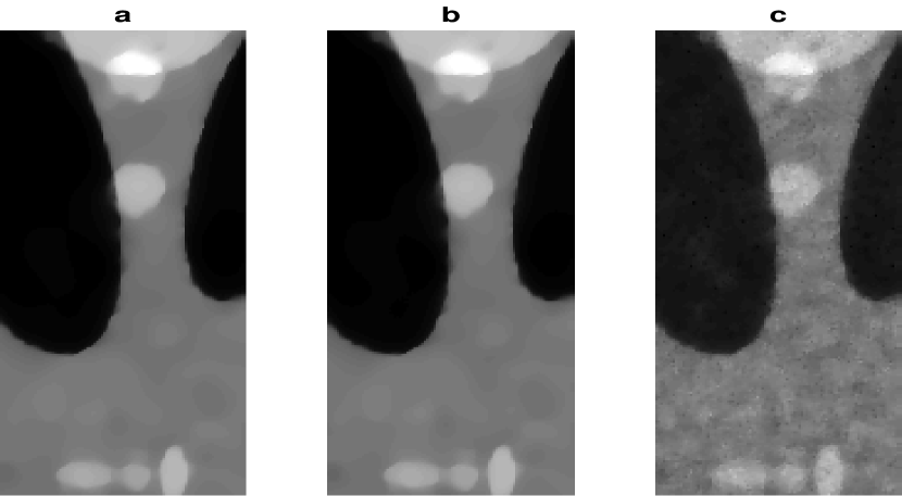
Figure 5: (a) 1000 iterations of the repeated TV filter, PSNR=28.50, (b) 135 iterations of the PCG accelerated TV filter, PSNR=28.48,
(c) 80 iterations of the Nesterov accelerated TV filter, PSNR=28.31

The preconditioned conjugate gradient acceleration may work especially well for the total variation denoising, when the graph Laplacian matrix is not properly scaled. Figure 6 shows results of the PCG accelerated TV denoising for the $512\times 512$-image liftingbody.png from MATLAB, corrupted by Gaussian noise with zero mean and variance 0.01. The PSNR value of the noisy image is 20.06.

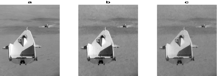
Figure 6: (a) clean image, (b) 800 iterations of the repeated TV filter, PSNR=33.18,
(c) 45 iterations of the PCG accelerated TV filter, PSNR=33.02

There exists a variant of acceleration proposed in [27], which is often called the heavy ball method. According to our numerical experience, we can conclude that the acceleration based on the heavy ball method is inferior to Nesterov’s acceleration.

We have also carried out extensive experiments with the BM3D code, developed by the authors of the BM3D method [15] and currently considered as one of the best patch-based denoising codes. BM3D with the default parameters usually requires only one application to reach the best possible quality. With other acceptable parameter choices, BM3D produces the best quality after 1 or 2 iterations. It means that our accelerations techniques are of no use for the BM3D code. However, we believe that our accelerations may be very useful for denoising signals and images on general graphs, where the patch-based methods do not work.

0.5 Conclusion

We have numerically demonstrated that acceleration by the preconditioned conjugate gradient and Nesterov’s methods works for the iterative self-guided smoothing filters in the 2D case. Both acceleration methods demonstrate similar efficiency. The accelerated filters achieve approximately the same denoising quality, e.g. in terms of PSNR, as the non-accelerated iterative application of basic filters such as the bilateral, guided, and total variation filters. The acceleration speedup, measured by the number of calls to basic smoothing filters, on images of moderate size, say $512\times 512$, can be in the range 2-12x. We remark that mathematical theory of the proposed accelerations of nonlinear smoothing filters is not developed yet. The accelerated filters may be especially useful for processing images and signals on general graphs.

References

- [1] P. Perona and J. Malik, “Scale-space and edge detection using anisotropic diffusion,” in Proc. IEEE Computer Society Workshop Computer Vision, Miami, FL, 1987, pp. 16–27.
- [2] P. Perona and J. Malik, “Scale-space and edge detection using anisotropic diffusion,” IEEE Trans. Pattern Analysis Machine Intelligence, vol. 12, no. 7, pp. 629–639, 1990, doi: 10.1109/34.56205.
- [3] V. Aurich and J. Weule, “Non-linear gaussian filters performing edge preserving diffusion,” in Mustererkennung 1995, 17. DAGM-Symposium, Bielefeld, Germany, 1995, pp. 538–545.
- [4] S. M. Smith and J. M. Brady, “SUSAN – A New Approach to Low Level Image Processing,” International J. Computer Vision, vol. 23, no. 1, pp. 45–78, 1997, doi: 10.1023/A:1007963824710.
- [5] C. Tomasi and R. Manduchi, “Bilateral filtering for gray and color images,” in Proc. IEEE International Conf. Computer Vision, Bombay, 1998, pp. 839–846, doi: 10.1109/ICCV.1998.710815.
- [6] M. Elad, “On the origin of the bilateral filter and ways to improve it,” IEEE Trans. Image Process., vol. 11, no. 10, pp. 1141–1151, 2002, doi: 10.1109/TIP.2002.801126.
- [7] S. Paris, P. Kornprobst, J. Tumblin, and F. Durand, “Bilateral filtering: Theory and applications,” Foundations and Trends in Computer Graphics, vol. 4, no. 1, pp. 1–73, 2009, doi: 10.1561/0600000020.
- [8] K. N. Chaudhury, “Acceleration of the shiftable O(1) algorithm for bilateral filtering and nonlocal means,” IEEE Transactions on Image Processing, vol. 22, no. 4, pp. 1291–1300, 2013, doi: 10.1109/TIP.2012.2222903.
- [9] K. Sugimoto and S.-I. Kamata, “Compressive bilateral filtering,” IEEE Transactions on Image Processing, vol. 24, no. 11, pp. 3357–3369, 2015, doi: 10.1109/TIP.2015.2442916.
- [10] K. He, J. Sun, and X. Tang, “Guided image filtering,” IEEE transactions on pattern analysis and machine intelligence, vol. 35, no. 6, pp. 1397–1409, 2013, doi: 10.1109/TPAMI.2012.213.
- [11] L. I. Rudin, S. Osher, and E. Fatemi, “Nonlinear total variation noise removal algorithms,” Physica D, vol. 60, no. 1-4, pp. 259–268, 1992. doi: 10.1016/0167-2789(92)90242-F.
- [12] O. Lezoray and L. Grady (eds.), “Image Processing and Analysis with Graphs. Theory and Practice,” CRC Press, Boca Raton, FL, 2012.
- [13] A. Buades, B. Coll, and J. M. Morel, “A review of image denoising algorithms, with a new one,” Multiscale Model. Simul., vol. 4, no. 2, pp. 490–530, 2005. doi: 10.1137/040616024.
- [14] C. Kervrann and J. Boulanger, “Optimal spatial adaptation for patch-based image denoising,” IEEE Trans. Image Process., vol. 15, no. 10, pp. 2866–2878, 2006. doi: 10.1109/TIP.2006.877529.
- [15] K. Dabov, A. Foi, V. Katkovnik, and K. Egiazarian, “Image denoising by sparse 3-d transform-domain collaborative filtering,” IEEE Trans. Image Process., vol. 16, no. 8, pp. 2080–2095, 2007, doi: 10.1109/TIP.2007.901238.
- [16] P. Chatterjee and P. Milanfar, “Patch-based near-optimal image denoising,” IEEE Trans. Image Process., vol. 21, no. 4, pp. 1635–1649, 2012. doi: 10.1109/TIP.2011.2172799.
- [17] M. Lebrun, M. Colum, A. Buades, and J. M. Morel, “Secrets of image denoising cuisine,” Acta Numerica, vol. 21, pp. 475–576, 2012. doi: 10.1017/S0962492912000062.
- [18] H. Talebi and P. Milanfar, “Global image denoising,” IEEE Trans. Image Process., vol. 23, no. 2, pp. 755–768, 2014, doi: 10.1109/TIP.2013.2293425.
- [19] H. Talebi and P. Milanfar, “Nonlocal image editing,” IEEE Trans. Image Process., vol. 23, no. 10, pp. 4460–4473, 2014, doi: 10.1109/TIP.2014.2348870.
- [20] A. Gadde, S.K. Narang, and A. Ortega, “Bilateral filter: Graph spectral interpretation and extensions,” in Proc. 20th IEEE International Conf. Image Processing (ICIP), Melbourne, Australia, 2013, pp. 1222–1226. doi: 10.1109/ICIP.2013.6738252.
- [21] D. Tian, A. Knyazev, H. Mansour, and A. Vetro, “Chebyshev and conjugate gradient filters for graph image denoising,” in Proc. IEEE International Conf. Multimedia Expo Workshops (ICMEW), Chengdu, 2014, pp. 1–6, doi: 10.1109/ICMEW.2014.6890711.
- [22] A. Knyazev and A. Malyshev, “Accelerated graph-based spectral polynomial filters,” Tech. Rep., 2015, arXiv:1509.02468.
- [23] A. Knyazev and A. Malyshev, “Conjugate gradient acceleration of non-linear smoothing filters,” Tech. Rep., 2015, arXiv:1509.01514.
- [24] K. Suwabe, M. Onuki, Y. Iizuka, and Y. Tanaka, “Globalized BM3D Using Fast Eigenvalue Filtering,” GlobalSIP 2015, Orlando, FL, USA, 2015. http://sigport.org/339
- [25] H. A. van der Vorst, Iterative Krylov Methods for Large Linear Systems, Cambridge University Press, Cambridge, UK, 2003, doi: 10.1017/CBO9780511615115.
- [26] A. V. Knyazev, “Toward the Optimal Preconditioned Eigensolver: Locally Optimal Block Preconditioned Conjugate Gradient Method,” SIAM J. Scientific Computing, vol. 23, no. 2, pp. 517–541,2001, doi: 10.1137/S1064827500366124.
- [27] B. T. Polyak, “Some methods of speeding up the convergence of iteration methods,” U.S.S.R. Comput. Math. Math. Phys., vol. 4, no. 5, pp. 1–17, 1964, doi: 10.1016/0041-5553(64)90137-5.
- [28] Y. E. Nesterov, “A method of solving a convex programming problem with convergence rate ,” Soviet Mathematics Doklady, vol. 27, no. 2, pp. 372–376, 1983.
- [29] W. Su, S. Boyd, and E. Candes, “A differential equation for modeling Nesterov’s accelerated gradient method: Theory and insights,” in Advances in Neural Information Processing Systems 27, Z. Ghahramani, M. Welling, C. Cortes, N.D. Lawrence, and K.Q. Weinberger, Eds., pp. 2510–2518. Curran Associates, Inc., 2014.