Finite temperature vortices in a rotating Fermi gas

Abstract

Vortices and vortex arrays have been used as a hallmark of superfluidity in rotated, ultracold Fermi gases. These superfluids can be described in terms of an effective field theory for a macroscopic wave function representing the field of condensed pairs, analogous to the Ginzburg-Landau theory for superconductors. Here, we have established how rotation modifies this effective field theory, by rederiving it starting from the action of Fermi gas in the rotating frame of reference. The rotation leads to the appearance of an effective vector potential, and the coupling strength of this vector potential to the macroscopic wave function depends on the interaction strength between the fermions, due to a renormalization of the pair effective mass in the effective field theory. The mass renormalization derived here is in agreement with results of functional renormalization group theory. In the extreme BEC regime, the pair effective mass tends to twice the fermion mass, in agreement with the physical picture of a weakly interacting Bose gas of molecular pairs. Then, we use our macroscopic wave function description to study vortices and the critical rotation frequencies to form them. Equilibrium vortex state diagrams are derived, and they are in good agreement with available results of the Bogoliubov – De Gennes theory and with experimental data.

I Introduction

Vortices and vortex matter in superconductors and superfluid atomic gases have been subjects of a great interest since a long time Bloch2008 . Stable vortices in superconductors appear under the presence of an external magnetic field. In superfluid atomic Bose and Fermi gases, vortices are stabilized when a trapped gas rotates, because the superfluid cannot support rigid-body rotation Stoof ; Iskin2009 . Stable vortices and vortex arrays were successfully generated experimentally in condensates of bosonic Matthews1999 ; Madison2000 ; Raman2001 ; Abo2001 and fermionic cold atoms Zwierlein2005 .

The experimental progress stimulated theoretical efforts to describe physics of vortex formation in rotating trapped quantum gases. Different theoretical methods were applied to describe the physics of the vortex matter in these systems: the Gross-Pitaevskii (GP) equation for Bose gases Fetter2009 ; Tsubota2002 , the Ginzburg - Landau (GL) formalism Bruun , the Bogoliubov - De Gennes (BdG) theory Machida ; Sensarma2006 ; Chien ; Simonucci2013 and the superfluid density functional theory Bulgac2013  for Fermi gases. The first calculation of the critical rotational velocity for a trapped Fermi gas has been performed in Ref. Bruun using a thermodynamic calculation of the energy of a vortex state. A similar calculation for the Bose gases was performed earlier in Ref. Dalfovo . The rotating Fermi condensates were investigated using macroscopic hydrodynamic equations in Refs. Cozzini ; Urban . In Refs. Warringa ; Warringa2 ; BdG-Wei2012 , the vortex formation in a rotating trapped Fermi gas is studied using the Bogoliubov - De Gennes (BdG) equations. In Ref. Simonucci2015 , vortex arrays in rotating Fermi condensates are analyzed using the coarse graining method for the BdG equations developed in Ref. Simonucci2014 , and referred to as a local phase density approximation (LPDA) to the BdG equations.

The BdG theory has been successfully extended to superfluid Fermi gases in the whole BCS-BEC crossover. However, from the computational point of view, the solution of the BdG equations for the fermionic wave functions is far more involved than the solution of, e. g., the Gross-Pitaevskii equation or any similar effective field approach describing the superfluid through a macroscopic wave function. As a result, the application of the BdG formalism is mostly limited to the zero-temperature properties of single-vortex states Machida ; Sensarma2006 ; Chien . To circumvent this limitation there has been a great interest in the development of effective field theories (EFT) which describe a superfluid system in terms of a macroscopic wave function (order parameter). The common key approximation for all branches of the EFT is the gradient expansion of the pair field, assuming it to be slowly varying in time and space. For example, the Ginzburg-Landau (GL) and the Gross-Pitaevskii (GP) theories can be considered as versions of the EFT, which are applicable in different ranges of parameters.

Effective field theories have been established for different cases in a number of works, see, e. g., Refs. Nishida ; Marini1998 ; Schakel ; KTD2014 ; Simonucci2014 , and used to describe non-uniform excitations (e. g., vortices, solitons) in Fermi gases in the BCS-BEC crossover. A notable example is the coarse-grained approximation to the static BdG formalism of Ref. Simonucci2014 , which allowed to extend the analysis to the whole temperature range below $T_{c}$.

The present study is based on the finite-temperature EFT for quantum gases in the BCS-BEC crossover formulated in our previous works. KTD ; KTLD2015 . This development of the EFT, based on a gradient expansion of the pairing order parameter at finite temperatures, is dynamic, accounting for both first-order and second-order time derivatives of the pair field. This allows to treat both equilibrium and time-dependent phenomena in superfluid Fermi gases. The gradient expansion is a common intrinsic element of an EFT. Therefore all advantages and shortcomings of this approach are not specific to the present work but are common for all EFTs (including GL and GP). Our derivation of the basic expressions of the finite temperature EFT KTD ; KTLD2015 is based on a straightforward extension of the first-nonvanishing-order expansion of the pair field action in powers of the pair field $\Psi$ by a complete exact summation of the series in powers of $\Psi$. It does not contain any additional hypothesis or model with respect to the well-established EFT derived previously for quantum gases in the BCS-BEC crossover near $T_{c}$, e. g., in Refs. Nishida ; Marini1998 ; Schakel ; deMelo1993 ; Diener2008 . The finite-temperature EFT has been tested by several successful applications to quantum gases KTLD2015 ; KTD2014 ; LAKT2015 which confirmed its validity.

The method described in Refs. KTD ; KTLD2015 was applied to solitons in a fermionic superfluid KTD2014 , where its advantage becomes clear: an analytic solution to the field equation is available. This approach will be referred to as KTD, and shown to compare successfully to the BdG formalism in the appropriate limit. Comparing this result to the numerical BdG simulations has shown that the effective field theory of KTD ; KTLD2015 is applicable throughout the BCS-BEC crossover except for the combination of the BCS regime and temperatures far below $T_{c}$ LAKT2015 , as expected (see the corresponding discussion in Ref. Simonucci2014 ).

In order to clearly indicate the place of the present work in the scientific context, we stress that extensions the BdG and Gor’kov theories which embrace BCS to BEC regimes for cold quantum gases were developed before in many works starting from the Nozières and Schmitt-Rink (NSR) scheme, see, e. g., Refs. NSR ; deMelo1993 . Within the Gaussian pair fluctuation approximation (GPF), the path integral description of BCS to BEC crossover treats the pairing channel at the level of the saddle point, and the Gaussian fluctuations are incorporated into a renormalized chemical potential. There is no real feedback of these fluctuations to the saddle point results as noted in Ref. Diener2008 . However the EFT that we developed in Refs. KTD ; KTLD2015 is not completely equivalent to the GPF approach. We go beyond GPF in what concerns the amplitude of the fluctuations: it is not assumed to be small.

A complementary approach for Fermi gases in the BCS-BEC crossover is based on the BCS-Leggett ground state Leggett ; Perali . The main difference between these two methods is that the NSR-based scheme reaches the BCS-BEC crossover by starting from the BEC limit, and the BCS-Leggett based scheme reaches this crossover by starting from the BCS limit (for a detailed comparison, see Ref. Levin ). Our recent works KTD ; KTLD2015 ; KTD2014 ; LAKT2015 lie within the context of the former.

The new elements of our version of the EFT, and, particularly, the message of the present paper can be described as follows. The GL approach with microscopically derived coefficients uses the pair field as a small parameter. Therefore it is valid only near $T_{c}$. On one hand, the extension of the GL approach for quantum gases valid near $T_{c}$ in the whole BCS-BEC crossover and at $T=0$ in the BEC limit was developed in Ref. deMelo1993 . On the other hand, an all-temperature extension of the GL method for BCS superconductors was developed by Tewordt and Werthammer Tewordt ; Werthammer using the gradient expansion for the order parameter. Our recent treatment KTD ; KTLD2015 partly fills an existing gap, finding a similar extension of the GL method for quantum gases in the BCS-BEC crossover.

Finally, the specific message of the present paper is an incorporation of rotation into the effective field theory of Refs KTD ; KTLD2015 . This is done in Sec. II by including the rotating potential at the level of the fermionic degrees of freedom, and deriving the modified EFT for the macroscopic wave function. As we will show, the vector potential of rotation contains the renormalization factor for the pair mass, which is in agreement with results of the functional renormalization group theory Diehl . In Sec. III, we show the equilibrium vortex state diagrams and determine the critical rotation frequencies as a function of temperature and interaction strength, compare the results with those of Refs. Warringa ; Warringa2 ; Simonucci2015 and analyze their connection with the experimental data Zwierlein2005 . Our results are summarized in Sec. IV.

II Effective field action

In the present work, we consider a rotating Fermi gas confined to an anisotropic parabolic trap described by the confinement frequencies $\omega_{j}$ ($j=x,y,z$) within the KTD approach described in Refs. KTD ; KTLD2015 and based on the path-integral description of the interacting Fermi gas. The Hubbard-Stratonovich transformation is used to introduce the bosonic pair field $\Psi$, and the action functional for these fields is obtained by integrating out the fermionic degrees of freedom. In the resulting action, a gradient expansion is performed, not around $\Psi=0$ as in the Ginzburg - Landau approach, but around the coordinate-dependent saddle-point value to be determined self consistently. The bosonic pair field is then interpreted as a macroscopic wave function for the superfluid pair condensate.

The regimes of validity of this method have been studied in detail in Ref. LAKT2015 . It is relevant to discuss once more the criteria of validity of the EFT in the present work. A necessary condition for the validity of this approach is the same as that for known effective field methods, e. g., the Ginzburg-Landau and Gross-Pitaevskii formalisms: the bosonic field $\Psi$ must vary sufficiently slowly in space and in time. This condition is consistent with a large number of particles in the superfluid system. Therefore we restrict the treatment to Fermi gases with a sufficiently large number of particles or sufficiently strong coupling in order to ensure $R_{j}\gg\xi$ and $R_{c,j}\gg\xi$, where $R_{j}=\left(\hbar/\left(m\omega_{j}\right)\right)^{1/2}$ is the characteristic scale for the trap potential along the $j$-th axis, $R_{c,j}$ is the size of the superfluid cloud along the same axis, and $\xi$ is the characteristic scale of non-uniform excitations. The parameter $\xi$ can then be interpreted as the healing length for these excitations, e. g., vortices or solitons.

In order to determine the range of applicability of the EFT, other length scales must also be taken into account, such as the particle spacing, the scattering length, and the pair size. Two of them are crucial for the criterion of applicability for effective field approaches: the healing length and the pair size. The latter one can be estimated through the pair coherence length $\xi_{pair}$ which was determined in THPistolesiStrinati ; THPalestiniStrinati through the pair correlation function of the fermion field operators $\psi_{\sigma}\left(\mathbf{r}\right),\psi_{\sigma}^{{\dagger}}\left(\mathbf{r}\right)$,

$$g_{\uparrow\downarrow}(\mathbf{r}) =-\left(\frac{n}{2}\right)^{2}+$$ (1)

$$+\left\langle\psi_{\uparrow}^{{\dagger}}\left(\mathbf{R}+\frac{\mathbf{r}}{2}\right)\psi_{\downarrow}^{{\dagger}}\left(\mathbf{R}-\frac{\mathbf{r}}{2}\right)\psi_{\downarrow}\left(\mathbf{R}-\frac{\mathbf{r}}{2}\right)\psi_{\uparrow}\left(\mathbf{R}+\frac{\mathbf{r}}{2}\right)\right\rangle,$$

using the definition

$$\xi_{pair}=\sqrt{\frac{\int d\mathbf{r}~{}r^{2}g_{\uparrow\downarrow}(\mathbf{r})}{\int d\mathbf{r}~{}g_{\uparrow\downarrow}(\mathbf{r})}}.$$ (2)

Effective field approaches are applicable when the pair size is small with respect to the size of a non-uniform solution itself, i. e., when $\xi_{pair}\ll\xi$ (see also the similar discussion in Ref. Simonucci2014 ). As found in Ref. LAKT2015 , the domain of applicability of the KTD effective field theory is extended with respect to the GL approach (valid at $T$ close to $T_{c}$) towards low temperatures, and with respect to the GP approach (valid in the BEC limit) towards BCS. The KTD effective field theory is thus not valid in the BCS regime combined with low temperatures $T\ll T_{c}$.

In order to incorporate rotation into the KTD approach, we first consider the single-particle Hamiltonian for a fermionic atom with mass $m$ confined to an anisotropic parabolic trap in the rotating frame of reference. The rotation leads to the appearance of the term $\left(-\omega\hat{L}_{z}\right)$ where $\omega$ is the rotation frequency and $\hat{L}_{z}$ is the $z$ component of the orbital angular momentum of the particle. Therefore the single-particle Hamiltonian in the rotating frame of reference is Gao2006 ; Urban2008 :

$$H=-\frac{\left(\nabla-i\mathbf{A}\left(\mathbf{r}\right)\right)^{2}}{2m}+\frac{m\left(\omega_{\perp}^{2}-\omega^{2}\right)}{2}\left(x^{2}+y^{2}\right)+\frac{m\omega_{z}^{2}}{2}z^{2},$$ (3)

with the rotational vector potential for fermions,

$$\mathbf{A}\left(\mathbf{r}\right)=m\left[\boldsymbol{\omega}\times\mathbf{r}\right],$$ (4)

and the rotation vector

$$\boldsymbol{\omega}\equiv\omega\mathbf{e}_{z}.$$ (5)

The effect of rotation in this Hamiltonian is explicitly subdivided to the Coriolis and centrifugal contributions. The Coriolis contribution results in the appearance of the vector potential (4), for which $\nabla_{\mathbf{r}}\cdot A=0$. The centrifugal potential leads to the softening of the confinement potential through $\omega_{\perp}^{2}\rightarrow\omega_{\perp}^{2}-\omega^{2}$. The trapped atomic configuration can be stable when $\omega_{\perp}^{2}-\omega^{2}>0$. In the context of our earlier assumption of a slowly varying field, the local density approximation is suitable to take into account the confinement for a rotating Fermi gas through a coordinate dependent chemical potential:

$$\mu_{\omega}\left(\mathbf{r}\right)=\mu_{0}-\frac{m\left(\omega_{\perp}^{2}-\omega^{2}\right)}{2}\left(x^{2}+y^{2}\right)-\frac{m\omega_{z}^{2}}{2}z^{2}.$$ (6)

This chemical potential enters the coordinate-dependent fermion density, which is determined from the local number equation. Note that a parabolic confinement potential facilitates the applicability of the effective field theory and of the local density approximation with respect to a confinement with sharp edges, e. g., a box potential. Moreover, faster rotation makes the confinement potential smoother, so that the rotation does not break up the applicability of the present method. The local density approximation for centrifugal and Coriolis contributions has, in general, the same range of applicability as described above.

Within the present treatment, both the superfluid and normal components of the Fermi gas are assumed to be in equilibrium in the rotating frame of reference. This approximation is used in many works, see, e. g., Refs. Warringa ; Warringa2 ; Simonucci2015 and references therein. Recently, it was argued that rotation may cause a phase separation between a nonrotating superfluid core and a rigidly rotating normal gas Iskin2009 . Also the cylindric rotation symmetry about the $z$ axis is broken in experiments due to a stirring field, which provides the rotation. The study of these effects is however beyond the scope of the present work.

Within the path-integral formalism of preceding works deMelo1993 ; Diener2008 and following to the scheme developed in Refs. KTD ; KTLD2015 , we start the treatment from the partition function of a fermionic system determined by the path integral over the fermionic fields,

$$\mathcal{Z}\propto\int\mathcal{D}\left[\bar{\psi},\psi\right]e^{-S}.$$ (7)

where the action functional $S$ is given by:

$$S=\int_{0}^{\beta}d\tau\int d\mathbf{r}\left[\sum_{\sigma=\uparrow,\downarrow}\bar{\psi}_{\sigma}\left(\frac{\partial}{\partial\tau}+H-\mu_{\sigma}\left(\mathbf{r}\right)\right)\psi_{\sigma}+g\bar{\psi}_{\uparrow}\bar{\psi}_{\downarrow}\psi_{\downarrow}\psi_{\uparrow}\right],$$ (8)

where $\beta=1/\left(k_{B}T\right)$, $T$ is the temperature, and $k_{B}$ is the Boltzmann constant. To allow for spin imbalance in the Fermi gas, chemical potentials $\mu_{\sigma}$ are introduced which can be different for “spin-up” and “spin-down” species. The coordinate dependent chemical potentials $\mu_{\sigma}$ are determined by (6) with $\mu_{0}\rightarrow\mu_{0,\sigma}$ for each component. The interaction energy with the coupling constant $g<0$ describes the model contact interactions between fermions as, for example, in Ref. deMelo1993 . It represents the Cooper pairing channel determined by the $s$-wave scattering between two fermions with antiparallel spins. The one-particle Hamiltonian $H$ in the rotating frame of reference is determined by formula (3).

A more detailed description of the derivation is given in Appendix A. After the Hubbard-Stratonovich transformation which introduces the bosonic pair fields $\left(\bar{\Psi},\Psi\right)$, integrating over the fermionic fields, and the gradient expansion for the pair field with a complete summation of the series in powers of $\left|\Psi\right|^{2}$ in each term of the gradient expansion, we arrive at the effective field action in the rotating reference frame,

$$S_{eff} =\int_{0}^{\beta}d\tau\int d\mathbf{r}\left\{\left[\Omega_{s}\left(w\right)+\frac{D}{2}\left(\bar{\Psi}\frac{\partial\Psi}{\partial\tau}-\frac{\partial\bar{\Psi}}{\partial\tau}\Psi\right)\right.\right.$$

$$+Q\frac{\partial\bar{\Psi}}{\partial\tau}\frac{\partial\Psi}{\partial\tau}-\frac{R}{2w}\left(\frac{\partial w}{\partial\tau}\right)^{2}+C\left(\nabla_{\mathbf{r}}\bar{\Psi}\cdot\nabla_{\mathbf{r}}\Psi\right)-E\left(\nabla_{\mathbf{r}}w\right)^{2}$$

$$\left.\left.+iD\mathbf{A}\cdot\left(\bar{\Psi}\nabla_{\mathbf{r}}\Psi-\Psi\nabla_{\mathbf{r}}\bar{\Psi}\right)\right]\right\}.$$ (9)

The coefficients of this effective field action and the thermodynamic potential $\Omega_{s}$ are determined in Appendix A. They can depend on coordinates through the squared amplitude of the pair field $w=\left|\Psi\right|^{2}$ and the chemical potentials $\mu=\left(\mu_{\uparrow}+\mu_{\downarrow}\right)/2$ and $\zeta=\left(\mu_{\uparrow}-\mu_{\downarrow}\right)/2$. The linear term in the gradient expansion appears due to rotation, because rotation breaks the local inversion symmetry. Note that this linear term is derived in a straightforward way, without any ad hoc assumption beyond the effective field approach.

It can be shown that the present approach is in agreement with well-established results of the functional renormalization group theory Boettcher ; Diehl in what concerns the effective pair mass. In the microscopic theory of superconductivity Gorkov1958 ; Gorkov1959 , the pair charge was determined as $e^{\ast}=2e$. As proven by Alben Alben1969 , the rotation of a superconductor brings a contribution to the vector potential with the same charge/mass ratio for a pair as for a free electron. Therefore the total vector potential of in the GL equation is twice the vector potential for an electron, both for rotating and non-rotating superconductors. In theories of rotating Fermi gases based on the GL or BdG equations Gao2006 ; Simonucci2015 , this principle is kept. Contrary to the GL or BdG based descriptions, effective field theories developed within the NSR-like formalism Marini1998 ; Nishida ; Schakel and within the renormalization group theory Boettcher ; Diehl necessarily contain the renormalized pair effective mass $m_{p}^{\ast}$, which tends to $2m$ only in the extreme BEC case. The present study lies within the latter of two aforesaid paradigms. Hence we will arrive at a renormalized pair mass.

The derivation of the renormalized pair mass for Fermi gases in the BCS-BEC crossover is described in Appendix A. It is shown that the renormalization factor $\tilde{e}$ (associated with the ratio of the effective pair mass to the fermion mass $\tilde{e}\equiv m_{p}^{\ast}/m$) is expressed through the coefficients of the effective action (9) by:

$${\tilde{e}}=\frac{1}{C}\frac{\partial\left(wD\right)}{\partial w}.$$ (10)

Fig. 1 conveys the fact that the present EFT is in line with well-established results of the functional renormalization group theory Boettcher ; Diehl . Here, the inverse of the renormalization factor, $1/\tilde{e}$, is plotted as a function of the inverse scattering length $1/\left(k_{F}a_{s}\right)$ (where $k_{F}$ is the Fermi wave vector) and the temperature, when $T$ passes from zero to $T_{c}$ for a three-dimensional Fermi gas confined to a cylindrically symmetric parabolic confinement potential, with the number of particles per unit length set to $N=1000$.

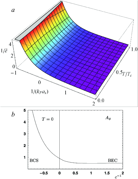
Figure 1: (Color online). (a) Inverse renormalization factor $1/\tilde{e}$ as a function of the dimensionless inverse scattering length $1/\left(k_{F}a_{s}\right)$ and the relative temperature $T/T_{c}$ for a three-dimensional Fermi gas in a cylindricaly symmetric parabolic confinement potential, with the number of particles per unit length $N=1000$. (b) Inverse renormalization factor obtained within the functional renormalization group theory Diehl for $T=0$. The renormalization factor $\tilde{e}$ is associated with the effective pair mass, as shown in Appendix A.

As seen from Fig. 1, the inverse renormalization factor only slightly depends on the temperature, and tends to 1/2 in the BEC limit, where the Fermi superfluid can be described as a Bose gas of molecules with the mass $m_{p}^{\ast}=2m$. Moving away from the BEC limit, $1/\tilde{e}$ gradually increases. The obtained behavior of the renormalization factor as a function of the inverse scattering length is in good agreement with the prediction of the functional renormalization group theory of Ref. Diehl . This is one of the key results of the present approach, which was not yet applied before to rotating Fermi gases. Thus, besides a renormalization of the chemical potential, an important element of the BCS-BEC crossover in the present work is a renormalization of all coefficients of the effective field action, including the renormalization of the pair mass.

Finally, the effective field action for a two-band system is straightforwardly determined in the same way as in Ref. KTLD2015 . We obtain action functionals for the separate fields, and a coupling given by an interband Josephson term:

$$S_{eff}^{\left(2b\right)}=\sum_{j=1,2}S_{eff}^{\left(j\right)}-\int_{0}^{\beta}d\tau\int d\mathbf{r~{}}\frac{\sqrt{m_{1}m_{2}}}{4\pi}\gamma\left(\bar{\Psi}_{1}\Psi_{2}+\bar{\Psi}_{2}\Psi_{1}\right),$$ (11)

Here $S_{eff}^{\left(j\right)}$ is the single-band effective field action for the $j$-th band determined by (9) with $j=1,2$, and $\gamma$ is the strength of the interband coupling. As derived in Ref. KTLD2015 , the coupling parameter $\gamma$ is fixed by the interband scattering lengths,

$$\gamma=2\left(\frac{1}{a_{s,3}}-\frac{1}{a_{s,4}}\right),$$ (12)

where the scattering lengths $a_{s,3}$ and $a_{s,4}$ are related to the interband scattering for the fermions with antiparallel and parallel spins, respectively.

III Vortex formation

In order to study the formation of vortices and vortex pairs in rotated superfluid Fermi gases, we use the amplitude-phase representation for the pair field similarly as in Refs. KTD2014 ; LAKT2015 ,

$$\Psi\left(\mathbf{r}\right)=\left|\Psi_{\infty}\right|a\left(\mathbf{r}\right)e^{i\theta\left(\mathbf{r}\right)}.$$ (13)

In this expression, $\left|\Psi_{\infty}\right|$ is the uniform background amplitude determined by solving gap and number equations for the uniform system. The amplitude modulation (the “hole” in the modulus of the order parameter at the vortex core) is modeled by the real function $a(\mathbf{r})$. The phase pattern is taken into account by $\theta(\mathbf{r})$ – for a vortex aligned with the $z$-axis, this is the angle around the $z$-axis. With this representation for $\Psi$, the free energy corresponding to the effective action becomes

$$F =\int d\mathbf{r}\left\{\left[\Omega_{s}\left(w\right)+\frac{1}{2}\rho^{\left(qp\right)}\left(\nabla_{\mathbf{r}}a\right)^{2}\right]\right.$$

$$\left.+\frac{1}{2}\rho^{\left(sf\right)}a^{2}\left(\nabla_{\mathbf{r}}\theta-\mathring{e}\mathbf{A}\right)^{2}-\frac{1}{2}\rho^{\left(sf\right)}\left(a\mathring{e}\mathbf{A}\right)^{2}\right\},$$ (14)

with

$$\rho^{\left(sf\right)} =2C\left|\Psi_{\infty}\right|^{2},$$ (15)

$$\rho^{\left(qp\right)} =2\left(C-4E\right)\left|\Psi_{\infty}\right|^{2}.$$ (16)

The parameters $\rho^{\left(sf\right)}$ and $\rho^{\left(qp\right)}$ represent, respectively, the superfluid density and the quantum pressure coefficient, as established in Refs. KTD2014 ; KTLD2015 . In order to find the conditions of stability for the vortex solutions, we consider the difference between two free energies:

$$\delta F\equiv F_{vortex}-F_{0}$$ (17)

where $F_{vortex}$ and $F_{0}$ are given by (14), respectively, with and without vortices. The bounds for the equilibrium vortex state diagrams with several vortex configurations are determined from the comparison of the free energies corresponding to these configurations.

From here on, we focus on vortex stability conditions for a one-band Fermi gas in three dimensions, trapped in a cylindrically symmetric parabolic potential characterized by the confinement frequency $\omega_{0}$, and rotating around the symmetry axis at a frequency $\omega$. We do not consider at the present stage the case when the population imbalance $\zeta$ is other than zero. The area of existence of vortices lies, in general, inside the area of existence for a superfluid state in a rotating Fermi gas. The latter one extends from the zero rotation frequency $\omega=0$ to a critical rotation frequency for the superfluid state $\omega_{\max}<\omega_{0}$. For $\omega>\omega_{\max}$, the system turns into the normal state Urban2008 ; Bausmerth2008 ; Veillette2006 .

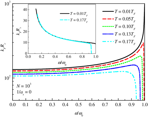
Figure 2: (Color online). Radius of the superfluid state as a function of the rotation frequency for a rotating Fermi gas with $1/a_{s}=0$ and $N=10^{3}$ confined to a cylindrically symmetric parabolic potential, at different temperatures. Inset shows the half-distance between vortex centers for a vortex pair at two temperatures.

Fig. 2 shows the behavior of the radius of the superfluid state $R_{c}$ and the half-distance between vortex centers $R_{v}$ for a vortex pair (inset) as a function of the relative rotation frequency $\omega/\omega_{0}$ for a rotating Fermi gas with $1/a_{s}=0$ and $N=10^{3}$ confined to a cylindrically symmetric parabolic potential. The dependence of the radius of the superfluid state versus $\omega$ is non-monotonic. When rotation gradually becomes faster but $\omega$ is not yet very close to its critical value $\omega_{\max}<\omega_{0}$ (where the superfluid state disappears), $R_{c}$ slowly increases, because the confinement weakens due to the centrifugal force. When $\omega$ is sufficiently close to $\omega_{\max}$, the superfluid core shrinks, turning to zero at $\omega=\omega_{\max}$. The critical value $\omega_{\max}$ decreases with increasing temperature, in accordance with the predictions of other works Warringa2 ; Veillette2006 .

Fig. 2 allows us to see also the temperature dependence of the size of the superfluid state and of the half-distance for the vortex pair. When $\omega$ is not close enough to $\omega_{\max}$, the radius $R_{c}$ decreases rather slowly with rising temperature. In the vicinity of $\omega_{\max}$, this decrease becomes much faster. The half-distance between vortices for a pair weakly depends on the temperature, except near $\omega_{\max}$, where $R_{v}$ falls together with $R_{c}$.

For a non-rotating Fermi gas and at sufficiently low rotation frequencies, vortices are not stable as long as the free energy (14) without vortices is lower than the free energy with vortices. When increasing $\omega$, vortices can become stable starting from a certain critical rotation frequency $\omega=\omega_{c,1}$. There may exist also an upper critical rotation frequency $\omega_{c,2}<\omega_{\max}$ such that the vortex state turns back to the superfluid state for $\omega_{c,2}<\omega<\omega_{\max}$. The appearance of an upper critical rotation frequency was also predicted by the BdG theory Warringa2 . The existence of a superfluid without any vortex at a fast rotation may seem counter-intuitive, but it has a transparent physical explanation. As seen from Fig. 2, starting from sufficiently large rotation frequencies, the radius of the superfluid state decreases. When the size of the superfluid is of the same order as the vortex size (or smaller), the formation of vortices can be not energetically favorable. This explains the existence of a superfluid without vortices at a fast rotation.

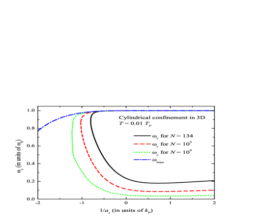
Figure 3: (Color online). Area of existence for vortices for a Fermi gas trapped in a cylindrically symmetric parabolic potential at $T=0.01T_{F}$, with different numbers of particles per unit length.

The area of existence for vortices for a system with different numbers of particles $N$ per unit length at $T=0.01T_{F}$ (where $T_{F}=E_{F}/k_{B}$) is shown in Fig. 3. When comparing our results with those of Ref. Warringa2 , one should note different units for the number of particles per unit length in that work than in the present treatment. Here, the lengths are measured in units of $1/k_{F}$, and in Ref. Warringa2 , the unit length is chosen as the oscillator length $l_{o}\equiv\left(\hbar/\left(m\omega_{0}\right)\right)^{1/2}$, where $\omega_{0}$ is the confinement frequency. We denote by $\mathcal{N}$ the number of particles per unit length according to Ref. Warringa2 , and ours by $N$. Therefore these two numbers are related to each other as $\mathcal{N}=N\mathcal{~{}}k_{F}l_{o}$. In our units, $l_{o}=\left(2/\omega_{0}\right)^{1/2}$ with $\omega_{0}=\sqrt{8/\left(15\pi N\right)}$, and hence $\mathcal{N}=\left(15\pi/2\right)^{1/4}N^{5/4}$. In particular, the value $N=134$ corresponds to $\mathcal{N}\approx 1000$ in Ref. Warringa2 .

We do not perform a quantitative comparison of the equilibrium vortex state diagrams calculated within the current approach with those obtained by the BdG method Warringa2 since the study in Ref. Warringa2 has been performed for the BCS regime, while the quantitative results of the current effective field theory, as discussed in Refs. KTLD2015 ; KTD2014 , are hardly applicable in the BCS regime at $T\ll T_{c}$. Nevertheless, the qualitative behavior of the boundary for the area of stable vortices is in agreement with the predictions of the BdG theory even in the BCS side. Particularly, we can see a bend-over of the critical rotation frequency and hence the existence of both a lower and an upper critical rotation frequency at weak coupling. At higher coupling strengths, the upper critical rotation frequency for the vortex formation tends to the critical rotation frequency for the superfluid state.

The region of vortex stability extends deeper into the BCS side and to smaller values of $\omega_{c,1}$ when increasing the number of particles. For sufficiently large $N\gtrsim 10^{4}$, stable vortices as predicted by the current formalism can be observed in the entire experimentally available BCS-BEC crossover region ($-1.2<1/\left(k_{F}a_{s}\right)<3.8$), in line with the experimental observations Zwierlein2005 . We have checked numerically that the lower critical rotation frequency $\omega_{c,1}$ for a single vortex in a Fermi gas with a large number of particles behaves in accordance with the estimation Bruun ; Nygaard :

$$\left.\omega_{c,1}\right|_{N\gg 1}\propto\omega_{B}\equiv\frac{1}{R_{c}^{2}}\ln\left(\frac{R_{c}}{\xi}\right),$$ (18)

where $R_{c}$ is the radius of the superfluid state in a trap, and $\xi$ is the healing length which characterizes the vortex size. The result of this numerical check is shown in Fig. 4. It shows the lower critical rotational frequency for a Fermi gas as a function of the number of particles per unit length and the ratio of the critical frequency compared to the analytic expression (18). We see that the ratio $\omega_{c,1}/\omega_{B}$ only slightly varies when $N$ passes from $N=10$ to $N=100$, so that the asymptotic trend (18) is clearly visible already when $N$ is not very large.

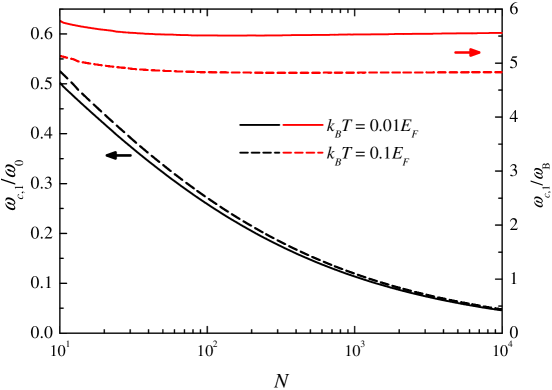
Figure 4: (Color online). Left-hand axis (indicated by the arrow for two lower curves): the lower critical rotation frequency $\omega_{c,1}$ (in units of the trapping potential parameter $\omega_{0}$) for a trapped Fermi gas as a function of the number of particles per unit length for $1/\left(k_{F}a_{s}\right)=0$, at two temperatures $k_{B}T=0.01E_{F}$ and $k_{B}T=0.1E_{F}$. Right-hand axis (indicated by the arrow for two upper curves): the ratio $\omega_{c}/\omega_{B}$ where $\omega_{B}$ is given by formula (18).

A similar asymptotic dependence for a Fermi gas trapped to a 3D spherically symmetric confinement potential was predicted in Ref. Bruun for a Fermi gas at zero temperature. In the present treatment, we find that the trend (18) is kept also at finite temperatures.

We can compare the obtained critical rotation frequency with the LPDA results of Ref. Simonucci2015 , using the parameters of the experimental setup of Ref. Riedl2011 where the unitary Fermi gas [$1/\left(k_{F}a_{s}\right)=0$] is trapped to an elongated trap with the confinement frequencies $\omega_{\perp}\approx 2\pi\times 680\operatorname{Hz}$ and $\omega_{z}\approx 2\pi\times 24\operatorname{Hz}$. When approximating this setup by a cylindrical confinement potential, we arrive at the number of particles per unit length $N\sim 10^{4}$. As seen from Fig. 4, for this number of particles, $\omega_{c,1}\approx 0.045$, which is in good agreement with the lower critical rotation frequency obtained in Ref. Simonucci2015 .

When the rotation frequency is increased beyond $\omega_{c,1}$, a second vortex may enter the superfluid. In the equilibrium vortex state diagram of Fig. 5, we distinguish the superfluid states with no vortex, one vortex and two or more vortices, in a trapped Fermi gas with $N=1000$ at the temperature $T=0.1T_{F}$. This temperature is higher than that for Fig. 3, and as a consequence the BCS-side boundary for vortex formation is found to shift to stronger coupling strengths. The boundary between the regimes with one and two vortices behaves similarly to the critical rotation frequency for a single vortex. It also exhibits a bend-over. The lower critical rotation frequency for a vortex pair is higher than the lower critical rotation frequency for a single vortex. On the contrary, the upper critical rotation frequency for a vortex pair is lower than the higher critical rotation frequency for a single vortex. Also the weak-coupling bound of $1/a_{s}$ for a single vortex lies more towards the BCS side with respect to that for a vortex pair. Thus the area where two or more stable vortices can exist lies entirely inside the area of stability for a single vortex.

In Fig. 6, we plot the equilibrium vortex state diagrams as a function of the variables $\left(\omega/\omega_{0},T/T_{c}\right)$ for two numbers of particles per unit length $N=10^{3}$ and $N=10^{4}$, and for three values of the inverse scattering length $1/\left(k_{F}a_{s}\right)=-0.5$ (the BCS case), $1/\left(k_{F}a_{s}\right)=0$ (unitarity), and $1/\left(k_{F}a_{s}\right)=1$ (the BEC case). It should be noted that different areas in the equilibrium vortex state diagrams do not refer to genuine thermodynamical phases, which are superfluid and normal phases. Also, equilibrium vortex state diagrams in a uniform superfluid (like ³He) would be different from those in a trapped Fermi gas.

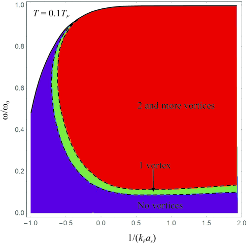
Figure 5: (Color online). Equilibrium vortex state diagram for a trapped rotating Fermi gas in a cylindrically symmetric parabolic confinement potential, showing the critical rotation frequencies as a function of the inverse scattering length for $T=0.1T_{F}$ and the number of particles per unit length $N=10^{3}$. The critical rotation frequencies are plotted for a single vortex and for a vortex pair. Also the upper bound for the rotation frequency is shown, which restricts the area of existence for the superfluid state.

In this equilibrium vortex state diagram, the transition lines between the regimes with no vortex, one vortex, and two or more vortices bend over leading to reentrant behavior of the critical rotation frequencies as a function of temperature. This reentrant dependence has a clear physical sense. On one hand, at higher temperatures, the radius of the superfluid phase (which is surrounded by the normal phase) decreases. On the other hand, the healing length, which determines the vortex size, increases when the temperature rises towards $T_{c}$. When the healing length is sufficiently large, the existence of stable vortices becomes energetically non-favorable with respect to the superfluid state. The obtained equilibrium vortex state diagrams exhibit a clear similarity to those obtained in Ref. Warringa2 (where they are calculated in the far BCS regime and at lower temperatures than those considered in the present work) and in Ref. Simonucci2015 . When moving from the BCS to the BEC regime, and when increasing the number of particles, the area for a single vortex, as well as the area for a superfluid state without vortices, become gradually narrower.

In Fig. 6, the temperature is measured in units of the critical temperature $T_{c}$ at the zero rotation. The critical temperatures calculated using the background chemical potential in the mean-field approach are overestimated with respect to experimental data, e. g., the mean-field value at unitarity $T_{c}\approx 0.4T_{F}$, while in the experiment Horikoshi , $T_{c}\approx 0.17T_{F}$. Taking Gaussian fluctuations into account Haussmann results in $T_{c}\approx 0.21T_{F}$ in better agreement with experimental estimate Horikoshi for the critical temperature. However, this will not qualitatively change the equilibrium vortex state diagrams when $T$ is scaled to $T_{c}$.

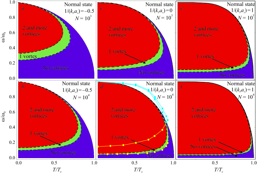
Figure 6: (Color online). Equilibrium vortex state diagrams for a trapped rotating Fermi gas in a cylindrically symmetric parabolic confinement potential, showing the critical rotation frequencies as a function of the temperature for two numbers of particles per unit length and three inverse scattering lengths (indicated in the figure). The notations are the same as in Fig. 5. Symbols in panel (d) show the critical rotation frequencies $\omega_{c,1}$ (dots) and $\omega_{c,2}$ (squares) from the Supplement to Ref. Simonucci2015 .

The equilibrium vortex state diagram shown in Fig. 6(d) corresponds to the same experimental setup as in Ref. Riedl2011 , theoretically considered in Ref. Simonucci2015 . For comparison, we plot there also the critical rotation frequencies $\omega_{c,1}$ and $\omega_{c,2}$ from Fig. S2 of the Supplement to Ref. Simonucci2015 , shown by symbols. The calculations in the present work are performed for a cylindrical confinement, which only approximately simulates an elongated trap considered in Ref. Simonucci2015 . Thus we expect only a qualitative agreement between our results and those of Ref. Simonucci2015 . However, the critical rotation frequencies in Fig. 6(d) appear to be close to those in the equilibrium vortex state diagram calculated within LPDA Simonucci2015 . It is also worth to note a good agreement between the KTD effective field theory and LPDA on the upper critical temperature for the vortex formation, as seen from Fig. 6(d).

There are also some differences between the critical rotation frequencies derived within these two approaches. In the BdG method, there are two definitions of the lower critical rotation frequency. A lower value of $\omega_{c,1}$ corresponds to the critical angular frequency at which an isolated vortex placed initially close to the trap center is attracted toward the trap center, while the upper value of $\omega_{c,1}$ corresponds to the critical rotation frequency at which an isolated vortex placed initially at the edge is attracted toward the trap center. This appearance of different critical rotation frequencies is apparently related to the fact that the LPDA equation determines a dynamic stability of vortices. In the EFT, the condition for the vortex formation follows from the comparison of the free energies with and without vortices. In other words, we consider only the thermodynamic stability of the vortex configurations. Therefore a single critical rotation frequency is obtained in the present work. The upper value of $\omega_{c,1}$ can thus correspond to a thermodynamically metastable configuration. As soon as the experimental preparation of the states of quantum atomic gases and the measurements are performed during a finite time, both thermodynamically stable and metastable configurations can be observable. Which critical rotation rate is relevant for a particular experiment depends on the way in which the experiment is performed.

According to the results shown in Figs. 4 and 6(d), the critical rotation frequency $\omega_{c,1}$ given by the present EFT is in excellent agreement with the lowest of two values of $\omega_{c,1}$ provided by the coarse grained BdG theory Simonucci2015 . This may shed light on which of the two values of $\omega_{c,1}$ indicated in Ref. Simonucci2015 corresponds to the thermodynamically stable state: the lower one is stable while the higher one can be thermodynamically metastable.

A comparison with the observations of vortices in the experiment of Ref. Zwierlein2005 indicates that the ranges of applicability of the BdG formalism combined with the Thomas-Fermi approximation Warringa ; Warringa2 and the KTD effective field theory are complementary to each other. The KTD field theory becomes more accurate towards the BEC regime KTLD2015 , while, as concluded in Ref. Warringa2 , the BdG method is quantitatively more reliable towards the BCS regime. It was found in Refs. Warringa ; Warringa2 that within the BdG theory, vortices in rotating Fermi gases are formed only for relatively large negative scattering lengths. On the contrary, the current formalism predicts the formation of stable vortices in rotating Fermi gases in the whole BCS-BEC crossover, in agreement with the experimental observations Zwierlein2005 .

The inverse scattering length was varied in the experiment of Ref. Zwierlein2005 in a wide range from $1/\left(k_{F}a_{s}\right)=-1.2$ to $1/\left(k_{F}a_{s}\right)=3.8$, and vortices were observed in the whole range of $1/\left(k_{F}a_{s}\right)$ between those values. In the experiment Zwierlein2005 , ⁶Li atoms were trapped in an approximately parabolic trap with the confinement frequencies $\omega_{\perp}\approx 2\pi\times 57\operatorname{Hz}$ and $\omega_{z}\approx 2\pi\times 23\operatorname{Hz}$. This gives us an estimation of the trap length along the $z$ axis $l_{z}\equiv\left(\hbar/\left(m\omega_{z}\right)\right)^{1/2}\approx 8.5\operatorname{\mu m}$. The total number of atoms was $N\propto 10^{6}$. Thus we can estimate the number of particles per unit length in order to qualitatively match the experiment as $N\propto N/l_{z}\propto 10^{4}$. The highest number of vortices at a given stirring frequency was obtained at $1/\left(k_{F}a_{s}\right)\approx 0.35$ which is rather close to the position of the minimum of the critical rotation frequency for $N=10^{4}$ in Fig. 3. It is hard to extract the critical rotation frequency for a single vortex from the experimental data of Ref. Zwierlein2005 . However, it is suggestive that the minimum of the critical rotation frequency and the maximum of vortices at a given (higher) rotation frequency lie close each other. Thus the above results of the present work are in line with the experiment Zwierlein2005 in what concerns the most favorable scattering length for the vortex formation in a rotating Fermi gas. Also, the estimate of the optimal rotation frequency within the modified finite temperature EFT is in a good agreement with the result of the coarse grained BdG theory Simonucci2015 and with the experiment Zwierlein2005 . This agreement is remarkable despite the fact that the rotation is incorporated in the LPDA equation of Ref. Simonucci2015 and in the present work in different ways.

IV Conclusions

In the present work, we extend the effective field theory developed in Refs. KTD ; KTLD2015 for fermionic superfluids to the case of rotating Fermi gases. The treatment is performed within the same path integral formalism as in the theoretical studies of cold quantum gases which embrace BCS to BEC regimes, performed in preceding works. The new physics in our recent works on the EFT is related to an extension of the GL theory below $T_{c}$ in the BCS-BEC crossover.

The rotation has been incorporated in the effective field action in a straightforward way, leading to the appearance of an effective vector potential as in other effective field theories. Therefore the physical picture, e. g., for the formation of vortices, is qualitatively one and the same in different formalisms (see, e. g., Warringa2 ; Simonucci2015 ). The new results consist in a concrete form of the coefficients of the EFT action, which are not phenomenological, but they are derived microscopically, starting from the initial fermionic Hamiltonian. Therefore, when describing the formation of vortices, the novelty consists in a quantitative description of the vortex system in a rotating trap.

One of the non-trivial physical results obtained in the present work is the fact that the vector potential of the rotation in the effective field action can be different from twice the vector potential for bare fermions. This difference is due to a renormalization of the effective mass for the pair field. It is directly related to the fact that the description of an interacting quantum atomic Fermi gas differs from the known BCS formalism for superconductors even in the BCS regime, that has been pointed out already in Ref. deMelo1993 .

In detail, the rotation leads to a shift in the local chemical potential $\mu_{\omega}$, and to the appearance of the rotational vector potential $\mathbf{A}$ in the covariant derivative $-i\nabla_{\mathbf{r}}\rightarrow-i\nabla_{\mathbf{r}}-\mathring{e}\mathbf{A}$, that leads to the renormalization factor $\tilde{e}$ in the equations of motion for the pair field. The renormalization factor tends to two in the BEC limit, in agreement with the physical picture of a molecular Bose gas with the boson mass $m_{p}^{\ast}=2m$. Moving away from the BEC limit, this value diminishes. The change of the renormalization factor from the BEC limiting value $\tilde{e}=2$ has a clear physical explanation. The fermion pair in a rotating Fermi condensate moves similarly to a point particle only in the deep BEC regime. However, beyond the BEC limit, the fermion pair cannot be considered as a point particle, especially in the BCS regime, where the Cooper-pair size is large. As a result, the pair effective mass diminishes when the inverse scattering length moves from BEC to the BCS side.

The renormalization of the effective mass that we obtain is in agreement with the preceding effective field theory of atomic Fermi gases, as checked by the comparison of the derived effective field action in particular cases $T\rightarrow T_{c}$ and $T\rightarrow 0$ with reliable works deMelo1993 ; Diener2008 ; Marini1998 ; Schakel . It is also in agreement with results of the functional renormalization group theory Diehl .

Using the obtained formalism, we investigate equilibrium vortex state diagrams where we identify regions for the superfluid state with no vortices, one vortex and two or more vortices. For the equilibrium vortex state diagrams in the variables $\left(\omega,1/a_{s}\right)$, the transition curves between these regions bend over in the BCS regime, in agreement with the results found using BdG calculations in this regime Warringa2 . As the number of particles is increased, the region of the equilibrium vortex state diagram where vortices are stable extends deeper into the BCS regime. Increasing the temperature, on the other hand, shrinks the region of stable vortices. The obtained dependence of the renormalization factor on the inverse scattering length is essential for these equilibrium vortex state diagrams, especially for sufficiently weak couplings.

The range of applicability of any kind of the effective field theory (including, e. g., GL and GP methods) is intrinsically related to the common assumption for them – that the order parameter smoothly varies in time and space. In what concerns the space variation, this means that the EFT can be applicable when the characteristic scale of the variation of the order parameter (e. g., the size of vortices or solitons) exceeds the Cooper-pair correlation length, as discussed in Ref. Simonucci2014 . The range of applicability of the present finite temperature EFT has been estimated quantitatively in Ref. LAKT2015 . The rotation considered in the present work does not crucially influence the range of applicability of the EFT.

The equilibrium vortex state diagrams in the variables $\left(\omega,T\right)$ exhibit clear similarity with the results of the BdG method (both the complete BdG Warringa ; Warringa2 and the coarse graining approximation for BdG Simonucci2015 ) where a good quantitative agreement has been found between the critical rotation frequencies obtained within the present theory and coarse-grained BdG. The lowest critical frequencies calculated in both EFT and LPDA approaches lie very close to each other despite the fact that our calculation lies within the NSR-like picture (where the effective mass of “dressed” pairs is renormalized) while the LPDA treatment is in agreement with the BCS-Leggett picture, where masses of pairs are non-renormalized. This coincidence is remarkable and may be useful to throw a bridge between these two paradigms.

We have also arrived at the optimal inverse scattering length for the vortex formation corresponding to the lowest critical rotation frequency. This value of the inverse scattering length is in a good agreement with the coupling strength at which the maximal number of vortices is generated in the experiment Zwierlein2005 .

In the present work, we considered the equilibrium configurations of vortices in rotating traps. The time-dependent phenomena can also be investigated within the EFT, in general combined with equations for the quasiparticle distributions. These equations are not an intrinsic part of the EFT and can be added as an independent ingredient. We have however treated some particular time-dependent phenomena (travelling dark solitons and collective excitations in quantum Fermi gases) in Refs. KTLD2015 ; KTD2014 , and the KTD effective field approach appears to be in line with the BdG theory and with experiments.

It is worth noting that an advantage of the present method with respect to the BdG theory is much shorter computational time and lower memory consumption. This advantage persists even with respect to the coarse-grained BdG, because the minimization of the free energy is substantially simpler and faster than a numerical solution of the differential equations. Moreover, effective field approaches allow for analytic solutions in many interesting cases, as shown in our work on dark solitons KTD2014 . Therefore it is planned to extend the treatment of non-linear excitations in condensed Fermi gases within the EFT, involving other factors of interest, such as spin imbalance, two-band Fermi gases, and spin-orbit coupling. The spin imbalance has been already incorporated analytically in the coefficients of the effective action (9), and the analysis of effects provided by the imbalance combined with the rotation is in progress. The spin-orbit coupling will be taken to account at the microscopic level similarly to Refs. SO . Finally, as shown in Sec. II, the extension of the present approach to two-band Fermi gases is straightforward.

The other ingredient which can be incorporated in the EFT is the account of induced interactions first considered by Gorkov and Melik-Barkhudarov GMB . Their importance for quantum gases in the BCS-BEC crossover was recently demonstrated Yu . The induced interactions lead to substantial corrections of the parameters of state in the BCS regime, while being less significant in the BEC regime. Therefore the account of induced interactions is expected to extend the range of applicability of the EFT towards weak coupling strengths and to improve a quantitative agreement between EFT and experiment.

Appendix A Incorporation of rotation in the effective field theory

A.1 Gradient expansion

The partition function of a fermionic system with two spin states ($\sigma=\uparrow,\downarrow$) is determined by the path integral over the fermionic fields ,

$$\mathcal{Z}\propto\int\mathcal{D}\left[\bar{\psi},\psi\right]e^{-S}.$$ (19)

where the action functional $S$ is given by:

$$S=\int_{0}^{\beta}d\tau\int d\mathbf{r}\left[\sum_{\sigma=\uparrow,\downarrow}\bar{\psi}_{\sigma}\left(\frac{\partial}{\partial\tau}+H-\mu_{\sigma}\left(\mathbf{r}\right)\right)\psi_{\sigma}+g\bar{\psi}_{\uparrow}\bar{\psi}_{\downarrow}\psi_{\downarrow}\psi_{\uparrow}\right],$$ (20)

where $\beta=1/\left(k_{B}T\right)$, $T$ is the temperature, and $k_{B}$ is the Boltzmann constant. To allow for spin imbalance in the Fermi gas, chemical potentials $\mu_{\sigma}$ are introduced which can be different for “spin-up” and “spin-down” species. The coordinate dependent chemical potentials $\mu_{\sigma}$ are determined by (6) with $\mu_{0}\rightarrow\mu_{0,\sigma}$ for each component. The interaction energy with the coupling constant $g<0$ describes the model contact interactions between fermions as, for example, in Ref. deMelo1993 . It represents the Cooper pairing channel determined by the $s$-wave scattering between two fermions with antiparallel spins. The one-particle Hamiltonian $H$ in the rotating frame of reference is determined by formula (3).

After performing the Hubbard-Stratonovich transformation which introduces the bosonic pair fields $\left(\bar{\Psi},\Psi\right)$, and integrating over the fermionic fields, the partition function becomes Stoof

$$\mathcal{Z}\propto\int\mathcal{D}\left[\bar{\Psi},\Psi\right]e^{-S_{eff}},$$ (21)

with the effective bosonic action $S_{eff}$:

$$S_{eff}=S_{B}-\operatorname{Tr}\left[\ln\left(-\mathbb{G}^{-1}\right)\right].$$ (22)

We decompose the inverse Nambu matrix $\mathbb{G}^{-1}$ into a sum of the matrix $\mathbb{F}$ proportional to the pair field $\Psi$, as in Ref. KTLD2015 ,

$$\mathbb{F}\left(\mathbf{r},\tau\right)=\left(\begin{array}[c]{cc}0&-\Psi\left(\mathbf{r},\tau\right)\\ -\bar{\Psi}\left(\mathbf{r},\tau\right)&0\end{array}\right),$$

and the free-field contribution,

$$\mathbb{G}_{0}^{-1}\left(\mathbf{r},\tau\right)=\left(\begin{array}[c]{cc}-\frac{\partial}{\partial\tau}-H+\mu_{\uparrow}&0\\ 0&-\frac{\partial}{\partial\tau}+H^{\ast}-\mu_{\downarrow}\end{array}\right).$$ (23)

In the momentum representation, the $\mathbb{G}_{0}$ is explicitly obtained from (23):

$$\mathbb{G}_{0}\left(\mathbf{k},n\right)=\left(\begin{array}[c]{cc}\frac{1}{i\omega_{n}-\xi_{\mathbf{k}}+\zeta_{\mathbf{k}}}&0\\ 0&\frac{1}{i\omega_{n}+\xi_{\mathbf{k}}+\zeta_{\mathbf{k}}}\end{array}\right)$$ (24)

with $\xi_{\mathbf{k}}=k^{2}/\left(2m\right)-\mu\left(\mathbf{r}\right)$ and

$$\zeta_{\mathbf{k}}=\zeta+2\mathbf{k}\cdot\mathbf{A}\left(\mathbf{r}\right),$$ (25)

where $\mu=\left(\mu_{\uparrow}+\mu_{\downarrow}\right)/2$ and $\zeta=\left(\mu_{\uparrow}-\mu_{\downarrow}\right)/2$. As discussed above, the coordinate-dependent vector potential is taken into account here in the local density approximation, assuming that $\mathbf{A}\left(\mathbf{r}\right)$ varies slowly, as does the trapping potential (which is included here through the coordinate dependent chemical potential). The above procedure is quite similar for Fermi gases in three and two dimensions.

Further on, we use the set of units with $\hbar=1$, $2m=1$, the Boltzmann constant $k_{B}=1$, and the Fermi energy for a free-particle Fermi gas $E_{F}\equiv\hbar^{2}k_{F}^{2}/\left(2m\right)=1$, where $k_{F}\equiv\left(3\pi^{2}n\right)^{1/3}$ is the Fermi wave vector and $n$ is the fermion density. Therefore in the present work, $k_{F}=1$, and the lengths are measured in units of $1/k_{F}$.

The next step is the gradient expansion of the effective action (22) following exactly the same scheme as in Ref. KTLD2015 , up to the second-order derivatives in time and in space. A complete summation in powers of the squared amplitude of the pair field $w\equiv\left|\Psi\right|^{2}$ is performed in each term of this gradient expansion separately. As a result, the following effective field action is obtained, which is structurally similar to that derived in Ref. KTLD2015 but with a new term provided by rotation:

$$S_{eff} =\int_{0}^{\beta}d\tau\int d\mathbf{r}\left\{\left[\Omega_{s}\left(w\right)+\frac{D}{2}\left(\bar{\Psi}\frac{\partial\Psi}{\partial\tau}-\frac{\partial\bar{\Psi}}{\partial\tau}\Psi\right)\right.\right.$$

$$+Q\frac{\partial\bar{\Psi}}{\partial\tau}\frac{\partial\Psi}{\partial\tau}-\frac{R}{2w}\left(\frac{\partial w}{\partial\tau}\right)^{2}+C\left(\nabla_{\mathbf{r}}\bar{\Psi}\cdot\nabla_{\mathbf{r}}\Psi\right)-E\left(\nabla_{\mathbf{r}}w\right)^{2}$$

$$\left.\left.+iG\mathbf{A}\cdot\left(\bar{\Psi}\nabla_{\mathbf{r}}\Psi-\Psi\nabla_{\mathbf{r}}\bar{\Psi}\right)\right]\right\}.$$ (26)

The coefficients in this effective field action (generalized here for a $\nu$-dimensional Fermi gas with $\nu=2,3$) take the form:

$$C =2\int\frac{d^{\nu}\mathbf{k}}{\left(2\pi\right)^{\nu}}\frac{k^{2}}{\nu}f_{2}\left(\beta,E_{\mathbf{k}},\zeta_{\mathbf{k}}\right),$$ (27)

$$D =\int\frac{d^{\nu}\mathbf{k}}{\left(2\pi\right)^{\nu}}\frac{\xi_{\mathbf{k}}}{w}\left[f_{1}\left(\beta,\xi_{\mathbf{k}},\zeta_{\mathbf{k}}\right)-f_{1}\left(\beta,E_{\mathbf{k}},\zeta_{\mathbf{k}}\right)\right],$$ (28)

$$E =\frac{4}{\nu}\int\frac{d^{\nu}\mathbf{k}}{\left(2\pi\right)^{\nu}}k^{2}~{}\xi_{\mathbf{k}}^{2}~{}f_{4}\left(\beta,E_{\mathbf{k}},\zeta_{\mathbf{k}}\right),$$ (29)

$$Q =\frac{1}{2w}\int\frac{d^{\nu}\mathbf{k}}{\left(2\pi\right)^{\nu}}\left[f_{1}\left(\beta,E_{\mathbf{k}},\zeta_{\mathbf{k}}\right)\right.$$

$$\left.-\left(E_{\mathbf{k}}^{2}+\xi_{\mathbf{k}}^{2}\right)f_{2}\left(\beta,E_{\mathbf{k}},\zeta_{\mathbf{k}}\right)\right],$$ (30)

$$R =\int\frac{d^{\nu}\mathbf{k}}{\left(2\pi\right)^{\nu}}\left[\frac{f_{1}\left(\beta,E_{\mathbf{k}},\zeta_{\mathbf{k}}\right)+\left(E_{\mathbf{k}}^{2}-3\xi_{\mathbf{k}}^{2}\right)f_{2}\left(\beta,E_{\mathbf{k}},\zeta_{\mathbf{k}}\right)}{3w}\right.$$

$$\left.+\frac{4\left(\xi_{\mathbf{k}}^{2}-2E_{\mathbf{k}}^{2}\right)}{3}f_{3}\left(\beta,E_{\mathbf{k}},\zeta_{\mathbf{k}}\right)+2E_{\mathbf{k}}^{2}wf_{4}\left(\beta,E_{\mathbf{k}},\zeta_{\mathbf{k}}\right)\right].$$ (31)

The functions $f_{p}\left(\beta,\varepsilon,\zeta\right)$ have been introduced in Ref. KTLD2015 . They are defined through fermionic Matsubara sums,

$$f_{p}\left(\beta,\varepsilon,\zeta\right)\equiv\frac{1}{\beta}\sum_{n=-\infty}^{\infty}\frac{1}{\left[\left(\omega_{n}+i\zeta\right)^{2}+\varepsilon^{2}\right]^{p}},$$ (32)

and have been expressed explicitly using the recurrence relations:

$$f_{1}\left(\beta,\varepsilon,\zeta\right) =\frac{1}{2\varepsilon}\frac{\sinh(\beta\varepsilon)}{\cosh(\beta\varepsilon)+\cosh(\beta\zeta)},$$ (33)

$$f_{p+1}\left(\beta,\varepsilon,\zeta\right) =-\frac{1}{2p\varepsilon}\frac{\partial f_{p}\left(\beta,\varepsilon,\zeta\right)}{\partial\varepsilon}.$$ (34)

The coordinate-dependent thermodynamic potential for a rotating Fermi gas is determined by the expressions:

$$\Omega_{s}\left(w\right) =-\int\frac{d\mathbf{k}}{\left(2\pi\right)^{3}}\left(\frac{1}{\beta}\ln\left(2\cosh\beta E_{\mathbf{k}}+2\cosh\beta\zeta_{\mathbf{k}}\right)\right.$$

$$\left.-\xi_{\mathbf{k}}-\frac{w}{2k^{2}}\right)-\frac{w}{8\pi a_{s}}\quad\left(\text{in 3D}\right),$$ (35)

and

$$\Omega_{s}\left(w\right) =-\int\frac{d^{2}\mathbf{k}}{\left(2\pi\right)^{2}}\left(\frac{1}{\beta}\ln\left(2\cosh\beta E_{\mathbf{k}}+2\cosh\beta\zeta_{\mathbf{k}}\right)\right.$$

$$\left.-\xi_{\mathbf{k}}-\frac{w}{2k^{2}+E_{b}}\right)\quad\left(\text{in 2D}\right),$$ (36)

where $E_{b}$ is the binding energy for a two-particle bound state in 2D.

Finally, when performing the gradient expansion, rotation leads to a new term in the effective field action (26), proportional to the first-order space gradient of the pair field,

$$\delta S_{eff}^{\left(rot\right)}=\int_{0}^{\beta}d\tau\int d\mathbf{r}~{}iG\mathbf{A}\cdot\left(\bar{\Psi}\nabla_{\mathbf{r}}\Psi-\Psi\nabla_{\mathbf{r}}\bar{\Psi}\right).$$ (37)

In the absence of rotation, this term vanishes due to inversion symmetry. It is calculated as in Ref. KTLD2015 , summing up the whole series in powers of the amplitude of the pair field in the coefficients at $\nabla\Psi$ and $\nabla\bar{\Psi}$. The new coefficient $G$, which appears due to the rotation, is:

$$G =D$$

$$+\int\frac{d^{\nu}\mathbf{k}}{\left(2\pi\right)^{\nu}}\frac{1}{w}\frac{\left(\mathbf{k\cdot A}\right)}{\left|\mathbf{A}\right|^{2}}\zeta_{\mathbf{k}}\left[f_{1}\left(\beta,\zeta_{\mathbf{k}},\xi_{\mathbf{k}}\right)-f_{1}\left(\beta,\zeta_{\mathbf{k}},E_{\mathbf{k}}\right)\right].$$ (38)

In summary, the effect of rotation on the effective field action functional derived in Ref. KTLD2015 is taken into account through the renormalization of the averaged chemical potential $\mu$ according to (6) and the replacement of the chemical potential imbalance as $\zeta\rightarrow\zeta_{\mathbf{k}}$. This may create a wrong impression that rotation can lead to polarized Fermi gases at $\zeta=0$. However, this is not the case. For clarity, let us consider a comparison between the real electromagnetic vector potential and the rotational vector potential. A real electromagnetic vector potential for particles with a true spin will lead to Zeeman splitting for spin states, so the chemical potentials of the two components can be different. The Zeeman splitting of “spin” states for atomic Fermi gases due to rotation is, in general, absent. On the contrary, splitting for the momentum states due to rotation occurs in the same way as due to a magnetic field Alben1969 . Moreover, this local-momentum splitting of the chemical potential appears in the Nambu tensor in the same way as in the Nambu-Gorkov theory. In order to see this, we can refer to the works Warringa ; Warringa2 ; Urban2008 , where the inverse Nambu matrix appears with the same one-particle Hamiltonian as in the present work. However, for a balanced gas, the contributions with $\zeta_{\mathbf{k}}$ and $\zeta_{-\mathbf{k}}$ cancel out in the integration over $\mathbf{k}$, and hence rotation does not lead to a population imbalance.

The appearance of the local-momentum splitting of the chemical potential is physically transparent. In a Cooper pair, the two fermions have opposite momenta. In the presence of rotation, their single-particle energies become unequal, in the same way as two pairing electrons in the magnetic field experience a Zeeman splitting. Note that for Cooper-paired electrons in a magnetic field, the Lorentz force destabilizes the pair already at much lower magnetic field than that where the Zeeman splitting breaks up the pair – however, for the neutral atoms, this effect is absent.

This physical picture assumes that the Cooper pair size is small with respect to a characteristic size of the superfluid system (for example, the radius of the trap) so that the background parameters within the extent of a Cooper pair are approximately uniform. This condition needs to be fulfilled in order for any description in terms of an effective field theory Nishida ; Marini1998 ; Schakel ; KTD2014 ; Simonucci2014 to be applicable. It should be noted that whereas the aforesaid splitting of the fermion energy is a standard result for the Bogoliubov - de Gennes theory, it has not been taken into account in existing effective field theories, so that this seems to be new with respect to other EFT-like approaches.

In accordance with Ref. Schakel , $G=D$ in (38) corresponds to the leading order and the term in the second line corresponds to the next-to-leading order in the effective field theory. Also the splitting $\zeta_{\mathbf{k}}$ of the chemical potential is the next-to-leading order correction with respect to the renormalization of $\mu$ due to rotation. Hence these corrections must be relatively small within the range of applicability of the effective field theory. Moreover, they should be neglected for consistency, because they may lead to non-controlled corrections beyond EFT.

A question may appear whether next-to-leading order terms can be important near a vortex core, where the order parameter rises rapidly. The range of applicability of the leading-order approximation is in fact the same as the range of applicability of any other effective field theory, e. g., the Ginzburg-Landau equation which is often used for the analysis of the vortices in superconductors and superfluids. This question is more general than the subject of the present study, because it is the same for rotating and non-rotating superfluids. It was studied in Refs. KTLD2015 ; LAKT2015 by a comparison of the obtained vortex parameters with results of the alternative microscopic approach – the BdG theory.

We can also show that next-to-leading order corrections should be neglected in order to satisfy the gauge invariance for the effective field action. In the derivation above, we start from the action for the fermionic field $\psi$ in the lab frame, then transform it to the rotating frame of reference, and finally perform the Hubbard-Stratonovich transformation to introduce the pair field $\Psi$. As a check of the gauge invariance of the obtained effective field action, we also consider inverting the order of these operations: first obtaining the action for the pair field $\Psi$ in gradient expansion, and then applying the transformation to the rotating frame of reference. In that case, the energy term $-\omega L_{z}$ (where $\hat{L}_{z}$ is the $z$ component of the orbital angular momentum for the pair field $\Psi$) appears in the bosonic pair Hamiltonian directly from the condition of the gauge invariance – similarly as in the Gross-Pitaevskii theory Stoof . This order of operations leads to the same final result as obtained above (9)-(40), but with the coefficient $G=D$. The resulting effective field action takes then the form:

$$S_{eff} =\int_{0}^{\beta}d\tau\int d\mathbf{r}\left\{\left[\Omega_{s}\left(w\right)+\frac{D}{2}\left(\bar{\Psi}\frac{\partial\Psi}{\partial\tau}-\frac{\partial\bar{\Psi}}{\partial\tau}\Psi\right)\right.\right.$$

$$+Q\frac{\partial\bar{\Psi}}{\partial\tau}\frac{\partial\Psi}{\partial\tau}-\frac{R}{2w}\left(\frac{\partial w}{\partial\tau}\right)^{2}+C\left(\nabla_{\mathbf{r}}\bar{\Psi}\cdot\nabla_{\mathbf{r}}\Psi\right)-E\left(\nabla_{\mathbf{r}}w\right)^{2}$$

$$\left.\left.+iD\mathbf{A}\cdot\left(\bar{\Psi}\nabla_{\mathbf{r}}\Psi-\Psi\nabla_{\mathbf{r}}\bar{\Psi}\right)\right]\right\}$$ (39)

The coefficients $D,C,E,Q,R$ in this effective field action are the same as in Ref. KTLD2015 . The new term $\left(\propto\mathbf{A}\right)$ expresses the coupling of the rotational vector potential to the current density.

A.2 Renormalization of the pair mass

The terms with the gradient of the pair field can be equivalently rewritten in terms of the covariant derivatives,

$$\int d\mathbf{r}\left[C\left(\nabla_{\mathbf{r}}\bar{\Psi}\cdot\nabla_{\mathbf{r}}\Psi\right)+iD\mathbf{A}\cdot\left(\bar{\Psi}\nabla_{\mathbf{r}}\Psi-\Psi\nabla_{\mathbf{r}}\bar{\Psi}\right)\right]$$

$$=\int d\mathbf{r}\left[C\left|\left(\nabla_{\mathbf{r}}-i\mathring{e}\mathbf{A}\right)\Psi\right|^{2}-C\mathring{e}^{2}A^{2}\left|\Psi\right|^{2}\right],$$ (40)

with the renormalization factor $\mathring{e}=D/C$. As established in Ref. KTLD2015 the coefficient $D$ enters the equations of motion for the pair fields only through the combination $\tilde{D}\equiv\partial\left(wD\right)/\partial w$. Consequently, physical sense can be attributed to the other renormalization factor,

$${\tilde{e}}=\frac{1}{C}\frac{\partial\left(wD\right)}{\partial w}.$$ (41)

The physical sense of the renormalization factor $\tilde{e}$ can be explained using the following reasoning. Let us temporarily, just for illustration purposes, neglect the terms with coefficients $E,Q,R$ (which are not necessary for this explanation) in the EFT action. In the absence of rotation, the equation of motion for the pair field in the real-time representation (simplifying the equation of motion from Ref. KTLD2015 ) then becomes:

$$i\frac{\partial\Psi}{\partial t}=-\frac{1}{2m_{p}^{\ast}}\nabla_{\mathbf{r}}^{2}\Psi+\frac{1}{\tilde{D}}\frac{\partial\Omega_{s}}{\partial w}\Psi,$$ (42)

with the effective mass of the pair

$$m_{p}^{\ast}\equiv\frac{\tilde{D}}{2C}.$$ (43)

This equation is similar to the Gross-Pitaevskii one, and is exactly reduced to the GP form if we expand the thermodynamic potential in powers of $\left|\Psi\right|^{2}$ up to the second order. In general, $m_{p}^{\ast}\neq 1$. This result is not surprising, because a renormalization of the effective pair mass with respect to twice the fermion mass can be straightforwardly obtained from the effective field actions of earlier works, e. g., Refs. deMelo1993 ; Huang . Note that in Ref. Huang it is explicitly stated that the effective boson mass is equal to unity only in the BEC limit. Moreover, the renormalization of the coefficients at the space gradients and time derivatives is predicted by the EFT formulated using the functional renormalization group method Boettcher ; Diehl .

The rotation can be incorporated in the GP-like equation (42) in the same way as in the Schrödinger equation – considering the Bose gas of pairs which is at rest in the rotating frame of reference. In the same way as described above for fermions, the rotation applied to (42) leads to the appearance of the rotational vector potential for the pair field

$$\mathbf{A}_{p}\left(\mathbf{r}\right)=m_{p}^{\ast}\left[\boldsymbol{\omega}\times\mathbf{r}\right].$$ (44)

Thus the renormalization factor $\tilde{e}=2m_{p}^{\ast}$ has the physical sense of the renormalized effective mass for the pair field in units of the fermion mass.

References

- (1) I. Bloch, J. Dalibard, and W. Zwerger, Rev. Mod. Phys. 80, 885 (2008).
- (2) H. T. C. Stoof, K. B. Gubbels, and D. B.M. Dickerscheid, Ultracold Quantum Fields (Springer, 2009).
- (3) M. Iskin and E. Tiesinga, Phys. Rev. A 79, 053621 (2009).
- (4) M. R. Matthews, B. P. Anderson,P. C. Haljan, D. S. Hall, C. E.Wieman, and E. A. Cornell, Phys. Rev. Lett. 83, 2498 (1999).
- (5) K. W. Madison, F. Chevy, W. Wohlleben, and J. Dalibard, Phys. Rev. Lett. 84, 806 (2000).
- (6) C. Raman, J.R. Abo-Shaeer, J.M. Vogels, K. Xu, and W. Ketterle, Phys. Rev. Lett. 87, 210402 (2001).
- (7) J. R. Abo-Shaeer, C. Raman, J. M. Vogels, and W. Ketterle, Science 292, 476 (2001).
- (8) M. W. Zwierlein, J. R. Abo-Shaeer, A. Schirotzek, C. H. Schunck, and W. Ketterle, Nature (London) 435, 1047 (2005)
- (9) M. Tsubota, K. Kasamatsu, and M. Ueda, Phys. Rev. A 65, 023603 (2002).
- (10) A. L. Fetter, Rev. Mod. Phys. 81, 647 (2009).
- (11) G. M. Bruun and L. Viverit, Phys. Rev. A 64, 063606 (2001).
- (12) M. Machida and T. Koyama, Phys. Rev. Lett. 94, 140401 (2005).
- (13) R. Sensarma, M. Randeria, and T.-L. Ho, Phys. Rev. Lett. 96, 090403 (2006).
- (14) C-C. Chien, Y. He, Q. Chen, and K. Levin, Phys. Rev. A 73, 041603 (2006).
- (15) S. Simonucci, P. Pieri, and G. C. Strinati, Phys. Rev. B 87, 214507 (2013).
- (16) A. Bulgac, Annu. Rev. of Nucl. Part. Sci. 63, 97 (2013).
- (17) F. Dalfovo and S. Stringari, Phys. Rev. A 53, 2477 (1996).
- (18) M. Cozzini and S. Stringari, Phys. Rev. Lett. 91, 070401 (2003).
- (19) M. Urban, Phys. Rev. A 71, 033611 (2005).
- (20) H. J. Warringa and A. Sedrakian, Phys. Rev. A 84, 023609 (2011).
- (21) H. J. Warringa, Phys. Rev. A 86, 043615 (2012).
- (22) R. Wei and E. J. Mueller, Phys. Rev. Lett. 108, 245301 (2012).
- (23) S. Simonucci, P. Pieri, and G. C. Strinati, Nature Physics 11, 941 (2015).
- (24) S. Simonucci and G. C. Strinati, Phys. Rev. B 89, 054511 (2014).
- (25) S. N. Klimin, J. Tempere, and J. T. Devreese, Phys. Rev. A 90, 053613 (2014).
- (26) M. Marini, F. Pistolesi, and G. C. Strinati, Eur. Phys. J. B 1, 151 (1998).
- (27) Y. Nishida and D. T. Son, Phys. Rev. A 74, 013615 (2006).
- (28) A. M. J. Schakel, Ann. Phys. 326, 193 (2011).
- (29) S. N. Klimin, J. Tempere, and J. T. Devreese, Physica C 503, 136 (2014).
- (30) S. N. Klimin, J. Tempere G. Lombardi, and J. T. Devreese, Eur. Phys. Journal B 88, 122 (2015).
- (31) C. A. R. Sá de Melo, M. Randeria, and J.R. Engelbrecht, Phys. Rev. Lett. 71, 3202 (1993).
- (32) R. B. Diener, R. Sensarma, and M. Randeria, Phys. Rev. A 77, 023626 (2008).
- (33) G. Lombardi, W. Van Alphen, S. N. Klimin, and J. Tempere, Phys. Rev. A 93, 013614 (2016).
- (34) P. Nozières and S. Schmitt-Rink, J. Low Temp. Phys. 59, 195 (1985).
- (35) A. J. Leggett, Nat. Phys. 2, 134 (2006).
- (36) A. Perali, P. Pieri, G. C. Strinati, and C. Castellani, Phys. Rev. B 66, 024510 (2002).
- (37) K. Levin, Q. Chen, C.-C. Chien, and Y. He, Ann. Phys. 325, 233 (2010).
- (38) L. Tewordt, Phys. Rev. 132, 595 (1963).
- (39) N. R. Werthammer, Phys. Rev. 132, 663 (1963).
- (40) S. Diehl and C. Wetterich, Nucl. Phys. B 770, 206 (2007).
- (41) F. Pistolesi and G. C. Strinati, Phys. Rev. B 49, 6356 (1994).
- (42) F. Palestini and G. C. Strinati, Phys. Rev. B 89, 224508 (2014).
- (43) M. Gao, H. Wu, and L. Yin, Phys. Rev. A 74, 023604 (2006).
- (44) M. Urban and P. Schuck, Phys. Rev. A 78, 011601 (R) (2008).
- (45) I. Boettcher, J. M. Pawlowski, and S. Diehl, Nucl. Phys. B, Proc. Suppl. 228, 63 (2012).
- (46) L. P. Gor’kov, Sov. Phys. JETP 7, 505 (1959).
- (47) L. P. Gor’kov, Sov. Phys. JETP 9, 1364 (1959).
- (48) R. Alben, Phys. Lett. 29A, 477 (1969).
- (49) I. Bausmerth, A. Recati, and S. Stringari, Phys. Rev. Lett. 100, 070401 (2008).
- (50) M. Y. Veillette, D. E. Sheehy, L. Radzihovsky, and V. Gurarie, Phys. Rev. Lett. 97, 250401 (2006).
- (51) N. Nygaard, G. M. Bruun, B. I. Schneider, C. W. Clark, and D. L. Feder, Phys. Rev. A 69, 053622 (2004).
- (52) S Riedl, E. R. Sánchez Guajardo, C. Kohstall, J. Hecker Denschlag, and R Grimm, New J. Phys. 13, 035003 (2011).
- (53) M. Horikoshi, S. Nakajima, M. Ueda, and T. Mukaiyama, Science 327, 442 (2010).
- (54) R. Haussmann and W. Zwerger, Phys. Rev. A 78, 063602 (2008).
- (55) J. P. A. Devreese, J. Tempere, and C. A. R. Sá de Melo, Phys. Rev. Lett. 113, 165304 (2014); Phys. Rev. A 92, 043618 (2015).
- (56) L. P. Gorkov and T. K. Melik-Barkhudarov, Sov. Phys. JETP 13, 1018 (1961).
- (57) Z.-Q. Yu, K. Huang, and L. Yin, Phys. Rev. A 79, 053636 (2009).
- (58) K. Huang, Z.-Q. Yu and L. Yin, Phys. Rev. A 79, 053602 (2009).