A Multi-Service Oriented Multiple-Access Scheme for Next-Generation Mobile Networks

Abstract

One of the key requirements for fifth-generation (5G) cellular networks is their ability to handle densely connected devices with different quality of service (QoS) requirements. In this article, we present multi-service oriented multiple access (MOMA), an integrated access scheme for massive connections with diverse QoS profiles and/or traffic patterns originating from both handheld devices and machine-to-machine (M2M) transmissions. MOMA is based on a) establishing separate classes of users based on relevant criteria that go beyond the simple handheld/M2M split, b) class dependent hierarchical spreading of the data signal and c) a mix of multiuser and single-user detection schemes at the receiver. Practical implementations of the MOMA principle are provided for base stations (BSs) that are equipped with a large number of antenna elements. Finally, it is shown that such a massive-multiple-input-multiple-output (MIMO) scenario enables the achievement of all the benefits of MOMA even with a simple receiver structure that allows to concentrate the receiver complexity where effectively needed.

I Introduction

In the aim of deploying the Internet of Things (IoT), designing a unified radio access technique for both machine-to-machine (M2M) communications and handheld mobile devices is a challenging problem. One major issue is the difference in terms of traffic patterns and QoS requirements [1] between these two types of communications. Another issue is the large number of IoT devices required to be simultaneously served. Further difficulties arise from the fact that M2M transmissions do not all have the same QoS profile and traffic characteristics [2, 3].

To address some of these challenges, the Third Generation Partnership Project (3GPP) has started to add M2M-type communications support into the radio access subsystem of LTE. Several proposals emerged within this work. Two of them are dubbed LTE for Machine-Type Communications (LTE-M) and Narrow-band LTE-M (NB LTE-M), each introducing a new user equipment (UE) category, the so-called Cat. 1.4MHz for LTE-M and Cat. 200kHz for NB LTE-M [4]. As their respective names indicate, these new UE categories restrict M2M transmissions to a small subband of the available bandwidth that is orthogonal to the broadband users. The same principle is used in Filtered-OFDM [5] with the difference that in Filtered-OFDM, subband-based filtering is applied to enable the use of a different transmission time interval (TTI) and OFDM numerology on the M2M subband. Other solutions consist in providing a separate network for M2M connections. Examples include LoRa${}^{\textrm{TM}}$ and SIGFOX${}^{\textrm{TM}}$ [1], which both operate in the unlicensed frequency bands. While the physical layer of SIGFOX${}^{\textrm{TM}}$ is based on frequency-division multiple access (FDMA) with ultra narrow band sub-channels, the technology adopted in LoRa${}^{\textrm{TM}}$ [6] employs is a mix of FDMA and of chirp spread spectrum [7]. However, none of the existing solutions is able to meet the following crucial requirements all at once.
1. Denser IoT deployment: The existing proposals offer significant improvement over current cellular standards in terms of support for IoT access but there is a need to support much larger numbers of simultaneous M2M transmissions. This goal should be met without sacrificing the QoS of broadband mobile services.
2. Multi-class users/services: Not enough attention has been paid to the different QoS and traffic profiles within the class of IoT devices. Indeed, many of these devices will not all be battery limited sensors and will not only emit small packets of data [2]. Moreover, there is a need to distinguish from within the services running on handheld devices those that have traffic characteristics and data rate requirements, e.g. short messages, previously considered to be typical of IoT services. Significant gains in resource utilization efficiency are expected from a multiple-access scheme that treats devices with different QoS profiles, whether handheld devices or IoT machines, as belonging to separate classes of users.
3. Flexibility in resource assignment: The new multiple-access scheme should be flexible in assigning resources to the different classes and to the different users within each class.
4. Efficiency in resource utilization: The new multiple-access scheme should be more efficient in resource utilization than the orthogonal schemes adopted in all the existing proposals.

II Multi-service Oriented Multiple Access

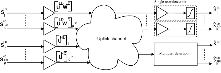
Figure 1: MOMA transmitters of two classes of users ($L=2$).

Consider a cell containing a base station (BS) required to serve $K$ users in the uplink. Assume that these users are grouped into $L\geq 2$ classes defined as follows.

• One maximum data rate (HD) class: Here, HD stands for “high data rate”. For this class the objective is to obtain a data rate as high as possible for a given number of users. Typically, these users are associated to data hungry applications on handheld devices.

• $\boldsymbol{L-1}$ constant data rate (LD) classes: Here, LD stands for “low data rate”. For these classes, the objective is to accommodate as many users as possible with granted data rates $r_{l}^{\mathrm{LD}}$ that satisfy

  $$r_{1}^{\mathrm{LD}}>r_{2}^{\mathrm{LD}}>\ldots>r_{L-1}^{\mathrm{LD}}\>.$$ (1)

  These users are typically associated with fixed low-rate transmissions from both handheld devices (such as short messages) and from different types of IoT services.

In the sequel, we use $\mathcal{K}^{\mathrm{HD}}\subset\{1,2,\ldots,K\}$ (resp. $\mathcal{K}_{l}^{\mathrm{LD}}$) to designate the indexes of the users of the HD (resp. the $l$-th LD) class. We also define $K^{\mathrm{HD}}\stackrel{{\scriptstyle\mathrm{def}}}{{=}}\left|\mathcal{K}^{\mathrm{HD}}\right|$, $K_{l}^{\mathrm{LD}}\stackrel{{\scriptstyle\mathrm{def}}}{{=}}\left|\mathcal{K}_{l}^{\mathrm{LD}}\right|$, $\mathcal{K}^{\mathrm{LD}}\stackrel{{\scriptstyle\mathrm{def}}}{{=}}\bigcup_{l\in\{1\cdots L-1\}}\mathcal{K}_{l}^{\mathrm{LD}}$, $K^{\mathrm{LD}}\stackrel{{\scriptstyle\mathrm{def}}}{{=}}\left|\mathcal{K}^{\mathrm{LD}}\right|$ and $\mathcal{K}\stackrel{{\scriptstyle\mathrm{def}}}{{=}}\mathcal{K}^{\mathrm{HD}}\cup\mathcal{K}^{\mathrm{LD}}$.

Since what matters for HD users is maximizing throughput, proper scheduling techniques will limit the number of simultaneously-transmitting users, thus it is reasonable to assume that $K^{\rm HD}$ will be small. This observation leads us to use multiuser detection techniques for this class of users. On the other hand, LD users will be quite numerous so that multiuser detection would be too complex. Therefore, we propose the use of single-user detection for this class of users. Moreover, to allow for high-performance HD connections, we want to limit interference from LD transmissions on HD received signals, we thus let HD and LD users to be quasi-orthogonal to each other. Lastly, this quasi-orthogonality is implemented in the code domain using a novel class-dependent hierarchical spreading scheme.

In the rest of this article we show how such a multiple-access scheme has the desirable property that the available radio resources are used in a flexible and efficient manner to allow connecting not only a large number of IoT devices, but also a large number of handheld devices running relatively low data rate services, while guaranteeing the satisfaction of the broadband services with high QoS requirements. This flexibility and efficiency in using the available resources is to be contrasted with the existing access solutions for IoT, such as LoRa${}^{\textrm{TM}}$, SIGFOX${}^{\textrm{TM}}$ and LTE-M, where the resources reserved for IoT services are under-used and their proportion to the overall resources cannot be dynamically adjusted.

III MOMA Transmitter

The MOMA transmitter ($L=2$) is illustrated in Fig. 1.

III-A Class Dependent Hierarchical Spreading

Let $\mathbf{U}$ be an orthogonal-code matrix, e.g. Walsh-Hadamard, whose columns are $N$-long spreading codes. In MOMA for $L$ classes of users, the set of columns of matrix $\mathbf{U}$ is divided into $L$ disjoint subsets that form $L$ matrices, namely $\mathbf{U}^{\mathrm{HD}}$ and $\{\mathbf{U}_{l}^{\mathrm{LD}}\}_{l\in\{1\cdots L-1\}}$ with respective dimensions $N\times N^{\mathrm{HD}}$ and $\{N\times N_{l}^{\mathrm{LD}}\}_{l\in\{1\cdots L-1\}}$. The $N^{\mathrm{HD}}$ spreading sequences of $\mathbf{U}^{\mathrm{HD}}$ will be assigned to $K^{\mathrm{HD}}$ HD users. Typically, $K^{\mathrm{HD}}\leq N_{l}^{\mathrm{LD}}$ so that the HD users could be scheduled in a quasi-orthogonal manner. This inequality could however be violated in the case where the spatial dimension is exploited, as we will see. The $N_{l}^{\mathrm{LD}}$ columns of $\mathbf{U}_{l}^{\mathrm{LD}}$ will be shared among the users of the $l$-th LD class. The scenario of interest for MOMA is when $K_{l}^{\mathrm{LD}}>N_{l}^{\mathrm{LD}}$, i.e. LD resources are overloaded, and when the following inequalities motivated by (1) are satisfied:

$$\frac{K_{L-1}^{\mathrm{LD}}}{N_{L-1}^{\mathrm{LD}}}>\cdots\frac{K_{1}^{\mathrm{LD}}}{N_{1}^{\mathrm{LD}}}>\frac{K^{\mathrm{HD}}}{N^{\mathrm{HD}}}\>.$$ (2)

The transmitted signals of the $K_{l}^{\mathrm{LD}}$ users within each LD class $l$ are formed by means of first linearly combining their data symbols using a rectangular combining matrix $\mathbf{W}_{l}^{\mathrm{LD}}$ of dimensions $N_{l}^{\mathrm{LD}}\times K_{l}^{\mathrm{LD}}$, before spreading the resulting symbols using the columns of matrix $\mathbf{U}_{l}^{\mathrm{LD}}$. Applying this class-dependent hierarchical spreading, the final spreading code $\mathbf{c}_{k}$ of a LD user $k$ can be written as

$$\mathbf{c}_{k}=\left[\mathbf{U}_{l}^{\mathrm{LD}}\mathbf{W}_{l}^{\mathrm{LD}}\right]_{j_{k}^{\mathrm{LD}}},\quad k\in\mathcal{K}_{l}^{\mathrm{LD}},l\in\{1\cdots L-1\}\>,$$ (3)

where $j_{k}^{\mathrm{LD}}\in\{1,2,\ldots,K_{l}^{\mathrm{LD}}\}$ is the index of the column of the matrix $\mathbf{U}_{l}^{\mathrm{LD}}\mathbf{W}_{l}^{\mathrm{LD}}$ assigned to user $k\in\mathcal{K}_{l}^{\mathrm{LD}}$ and where $\left[\mathbf{M}\right]_{i,j}$ designates the $i$-th element of the $j$-th column of matrix $\mathbf{M}$. In principle, $\mathbf{W}_{l}^{\mathrm{LD}}$ could be any $N_{l}^{\mathrm{LD}}\times K_{l}^{\mathrm{LD}}$ matrix chosen such that the transmit power constraint is respected:

$$\forall j\in\mathcal{K}_{l}^{\mathrm{LD}},\sum_{u=1}^{N_{l}^{\mathrm{LD}}}\left|\left[\mathbf{W}_{l}^{\mathrm{LD}}\right]_{u,j}\right|^{2}=1\>.$$ (4)

In the following, we assume that the components of $\mathbf{W}_{l}^{\mathrm{LD}}$ are chosen as realizations of independent and identically distributed (i.i.d.) random variables that can take the values $+\frac{1}{\sqrt{N_{l}^{\mathrm{LD}}}}$ and $-\frac{1}{\sqrt{N_{l}^{\mathrm{LD}}}}$ with equal probabilities. In contrast to LD users, no combining is applied to the symbols of the users from the HD class. The spreading code $\mathbf{c}_{k}$ used on the signals of a user $k\in\mathcal{K}^{\mathrm{HD}}$ can thus be written as

$$\mathbf{c}_{k}=\left[\mathbf{U}^{\mathrm{HD}}\right]_{j_{k}^{\mathrm{HD}}},\quad k\in\mathcal{K}^{\mathrm{HD}}\>,$$ (5)

where $\left[\mathbf{M}\right]_{j}$ designates the $j$-th column of matrix $\mathbf{M}$ and where $j_{k}^{\mathrm{HD}}\in\{1,2,\ldots,K^{\mathrm{HD}}\}$ is the index of the code assigned to user $k\in\mathcal{K}^{\mathrm{HD}}$ from among the columns of $\mathbf{U}^{\mathrm{HD}}$.

Remark 1.

Class dependent hierarchical spreading is distinct from the 2-step spreading (the so-called channelization and scrambling steps [8]) used in third-generation (3G) systems. Indeed, multiplication with $\mathbf{W}_{l}^{\mathrm{LD}}$ is intended to precondition signals from a number of users so that they can be spread using a much smaller number of orthogonal codes. This operation is thus completely unrelated, in its conception and in its purpose, to both channelization and scrambling in 3G.

III-B MOMA-OFDM

An orthogonal frequency division multiplexing (OFDM) implementation of MOMA (that we designate as MOMA-OFDM) consists in mapping the $N$ symbols from users’ spread signals to $N\leq N_{\mathrm{FFT}}$ consecutive subcarriers (SCs) in one OFDM symbol, where $N_{\mathrm{FFT}}$ is the total number of SCs per OFDM symbol. Let $\mathcal{N}$ be a subset of SCs chosen such that $\left|\mathcal{N}\right|=N$. Let $P_{k}$ designate the average transmit power of user $k\in\mathcal{K}$ . The signal transmitted by user $k$ on subcarrier $n\in\mathcal{N}$ is given by

$$x_{k,n}=\sqrt{P_{k}}\left[\mathbf{c}_{k}\right]_{n}s_{k}\>,$$ (6)

where $\left[\mathbf{c}_{k}\right]_{n}$ designates the component of $\mathbf{c}_{k}$ mapped to subcarrier $n$ and where $s_{k}$ is the zero-mean unit-variance data symbol transmitted by user $k$. Spreading codes $\mathbf{c}_{k}$ should be normalized such that $\mathbb{E}\left[\left|x_{k,n}\right|^{2}\right]=\frac{P_{k}}{N}$. MOMA-OFDM combines the benefits of both frequency-domain spreading, e.g. the ability to harvest the frequency diversity of the channel and the robustness against carrier frequency shifts, and of OFDM transmission, e.g. robustness against timing errors.

III-C MOMA with Massive MIMO Base Stations

We now turn our attention to the case where BS is equipped with a large number $M>>1$ of antennas while each user is equipped with a single antenna. This massive MIMO scenario, which is expected to be prevalent in 5G networks, proves to be particularly advantageous for MOMA, from both the performance and the receiver complexity perspectives. We designate this implementation of MOMA as MIMO-MOMA. Due to the spatial multiplexing capabilities inherent to this scenario, the number of HD users would typically be larger than the number of available HD orthogonal codes, i.e. $K^{\mathrm{HD}}>N^{\mathrm{HD}}$. The $N^{\mathrm{HD}}$ columns of matrix $\mathbf{U}^{\mathrm{HD}}$ should thus be shared among the $K^{\mathrm{HD}}$ HD users in such a way that each column is reused by $\left\lceil K^{\mathrm{HD}}/N^{\mathrm{HD}}\right\rceil$ users.

IV MOMA Receiver

Denote by $\mathbf{h}_{k,n}$ the vector of frequency-domain small-scale fading coefficient at subcarrier $n$ between user $k$ and the $M$ antennas of the BS during the current OFDM symbol and assume that the components of $\mathbf{h}_{k,n}$ are zero-mean i.i.d. random variables and that $\forall a\in\{1,2,\ldots,M\},\forall k\in\mathcal{K}$, $\forall n,m\in\mathcal{N}$, $\mathbb{E}\left[\left[\mathbf{h}_{k,n}\right]_{a}^{*}\left[\mathbf{h}_{k,m}\right]_{a}\right]=c_{n-m}^{h}$ where $\{c_{u}^{h}\}_{u\in\mathbb{Z}}$ is a frequency domain autocorrelation sequence. Finally, assume that coefficients $\mathbf{h}_{k,n}$ can be estimated at the BS by relying on uplink pilot sequences sent by the different user terminals. The vector $\mathbf{y}_{n}$ of samples received at the $M$ BS antennas at subcarrier $n$ is given by

$$\mathbf{y}_{n}=\sum_{k\in\mathcal{K}}\sqrt{g_{k}P_{k}}\mathbf{h}_{k,n}\left[\mathbf{c}_{k}\right]_{n}s_{k}+\mathbf{v}_{n}\>,$$ (7)

where $\mathbf{v}_{n}$ is a $M\times 1$ vector of i.i.d. $\mathcal{CN}\left(0,\sigma^{2}\right)$ noise samples and $g_{k}$ is the large-scale fading factor. The proposed receiver scheme consists in performing the following operations.

Spatial demultiplexing We propose the use of linear receive combining, e.g. according to maximum-ratio (MRC) or minimum-mean-square-error (MMSE) criteria. Combining with coefficients $\mathbf{d}_{k,n}$ provides the samples $r_{k,n}\stackrel{{\scriptstyle\mathrm{def}}}{{=}}\frac{1}{M}\mathbf{d}_{k,n}^{\mathrm{H}}\mathbf{y}_{n}$:

$$r_{k,n}=\sqrt{g_{k}P_{k}}\left[\tilde{\mathbf{c}}_{k}\right]_{n}s_{k}+\sum_{j\neq k}\sqrt{g_{j}P_{j}}\left[\tilde{\mathbf{c}}_{j}\right]_{n}s_{j}+\left[\tilde{\mathbf{v}}_{k}\right]_{n}\>,$$ (8)

where we defined for any $k,j\in\mathcal{K}$ and $\{n_{1},n_{2},\ldots,n_{N}\}=\mathcal{N}$

$$\tilde{\mathbf{c}}_{j}\stackrel{{\scriptstyle\mathrm{def}}}{{=}}\frac{1}{M}\left[\mathbf{d}_{k,n_{1}}^{\mathrm{H}}\mathbf{h}_{j,n_{1}}\left[\mathbf{c}_{j}\right]_{n_{1}}\cdots\mathbf{d}_{k,n_{N}}^{\mathrm{H}}\mathbf{h}_{j,n_{N}}\left[\mathbf{c}_{j}\right]_{n_{N}}\right]^{\mathrm{T}}$$ (9)

$$\tilde{\mathbf{v}}_{k}\stackrel{{\scriptstyle\mathrm{def}}}{{=}}\frac{1}{M}\left[\mathbf{d}_{k,n_{1}}^{\mathrm{H}}\mathbf{v}_{n_{1}}\cdots\mathbf{d}_{k,n_{N}}^{\mathrm{H}}\mathbf{v}_{n_{N}}\right]^{\mathrm{T}}$$ (10)

In the general case where $\{h_{k,n}\}_{n\in\mathcal{N}}$ are not fully correlated, users’ channels are selective in frequency. This implies that the effective spreading codes $\tilde{\mathbf{c}}_{k}$ and $\tilde{\mathbf{c}}_{j}$ of users $k$ and $j$ from two different classes are no longer orthogonal.

Remark 2 (Channel Hardening).

The effect of receive combining is averaging out small-scale fading over the array, in the sense that the variance of the effective scalar channel gain $\frac{1}{M}\mathbf{d}_{k,n}^{\mathrm{H}}\mathbf{h}_{k,n}$ decreases with $M$. This effect is known as channel hardening and is a consequence of the law of large numbers [10]. the frequency response $\frac{1}{M}\mathbf{d}_{k,n}^{\mathrm{H}}\mathbf{h}_{k,n}$ of the effective channel is thus asymptotically flat with $M$ and the above-mentioned loss of orthogonality vanishes.

HD Users Detection: In order to obtain HD data rates that are as high as possible, multiuser detection should be used. However, we limit the use of multiuser detection to cases where it is effectively needed. We know from the literature [9] that, under the assumption of uncorrelated antenna channel coefficients, the effective HD spreading gain is $MN^{\mathrm{HD}}$. Therefore, we propose the use of MMSE with successive interference cancellation (SIC) only in the case where $K^{\mathrm{HD}}\sim MN^{\mathrm{HD}}$, as opposed to $K^{\mathrm{HD}}\ll MN^{\mathrm{HD}}$ for which single-user detection should be sufficient. Define $\mathbf{A}\stackrel{{\scriptstyle\mathrm{def}}}{{=}}\mathrm{diag}\left\{\sqrt{P_{k}g_{k}}\right\}_{k\in\mathcal{K}^{\mathrm{HD}}}$ and the matrix $\tilde{\mathbf{C}}$ of effective codes as $\tilde{\mathbf{C}}\stackrel{{\scriptstyle\mathrm{def}}}{{=}}\left[\tilde{\mathbf{c}}_{k_{1}}\cdots\tilde{\mathbf{c}}_{k_{K^{\mathrm{HD}}}}\right]$, where $\{k_{1},k_{2},\ldots,k_{K^{\mathrm{HD}}}\}=\mathcal{K}^{\mathrm{HD}}$. Now assume that the columns of $\mathbf{A}$ and $\tilde{\mathbf{C}}$ are arranged in the descending order with respect to the values $\sqrt{P_{k}g_{k}}$ and define $\mathbf{T}\stackrel{{\scriptstyle\mathrm{def}}}{{=}}\tilde{\mathbf{C}}\mathbf{A}$. The MMSE-SIC receiver starts by recovering the symbol of user $k_{1}$ for which the value $\sqrt{P_{k_{1}}g_{k_{1}}}$ is the largest by computing $r_{k_{i}}^{\mathrm{HD}}\stackrel{{\scriptstyle\mathrm{def}}}{{=}}\boldsymbol{\delta}_{k_{i}}^{\mathrm{H}}\mathbf{r}_{k_{i}}$ where $\boldsymbol{\delta}_{k}\stackrel{{\scriptstyle\mathrm{def}}}{{=}}\left(\mathbf{T}\mathbf{T}^{\mathrm{H}}+\left(\sigma^{2}+\sum_{j\in\mathcal{K}^{\mathrm{LD}}}g_{j}P_{j}\right)/M\mathbf{I}\right)^{-1}[\mathbf{T}]_{k}$ and

$$\begin{multlined}(K^{\mathrm{HD}}\sim MN^{\mathrm{HD}})\quad r_{k_{i}}^{\mathrm{HD}}=\sqrt{g_{k_{i}}P_{k_{i}}}\boldsymbol{\delta}_{k_{i}}^{\mathrm{H}}\tilde{\mathbf{c}}_{k_{i}}s_{k_{i}}+\boldsymbol{\delta}_{k_{i}}^{\mathrm{H}}\tilde{\mathbf{v}}_{k_{i}}+\\ \sum_{j=i+1}^{K^{\mathrm{HD}}}\sqrt{g_{k_{j}}P_{k_{j}}}\boldsymbol{\delta}_{k_{i}}^{\mathrm{H}}\tilde{\mathbf{c}}_{k_{j}}s_{k_{j}}+\sum_{j\in\mathcal{K}^{\mathrm{LD}}}\sqrt{g_{j}P_{j}}\boldsymbol{\delta}_{k_{i}}^{\mathrm{H}}\tilde{\mathbf{c}}_{j}s_{j}\>,\end{multlined}(K^{\mathrm{HD}}\sim MN^{\mathrm{HD}})\quad r_{k_{i}}^{\mathrm{HD}}=\sqrt{g_{k_{i}}P_{k_{i}}}\boldsymbol{\delta}_{k_{i}}^{\mathrm{H}}\tilde{\mathbf{c}}_{k_{i}}s_{k_{i}}+\boldsymbol{\delta}_{k_{i}}^{\mathrm{H}}\tilde{\mathbf{v}}_{k_{i}}+\\ \sum_{j=i+1}^{K^{\mathrm{HD}}}\sqrt{g_{k_{j}}P_{k_{j}}}\boldsymbol{\delta}_{k_{i}}^{\mathrm{H}}\tilde{\mathbf{c}}_{k_{j}}s_{k_{j}}+\sum_{j\in\mathcal{K}^{\mathrm{LD}}}\sqrt{g_{j}P_{j}}\boldsymbol{\delta}_{k_{i}}^{\mathrm{H}}\tilde{\mathbf{c}}_{j}s_{j}\>,$$ (11)

for $k_{i}=k_{1}$ and $\mathbf{r}_{k_{1}}\stackrel{{\scriptstyle\mathrm{def}}}{{=}}\left[r_{k_{1},n_{1}}r_{k_{1},n_{2}}\cdots r_{k_{1},n_{N}}\right]^{\mathrm{T}}$. Once $s_{k_{1}}$ is decoded correctly, the contribution of $k_{1}$ can be removed from $\{r_{k_{2},n}\}_{n\in\mathcal{N}}$ in order to detect the data symbol of user $k_{2}$. The $N$-long vector of signal samples after this cancellation is denoted as $\mathbf{r}_{k_{2}}$. This SIC procedure continues till the detection of all the HD data symbols. In the case where $K^{\mathrm{HD}}<<M\times N^{\mathrm{HD}}$, MMSE-SIC is dropped and single-user (SU) detection is instead used by computing $r_{k}^{\mathrm{HD,SU}}\stackrel{{\scriptstyle\mathrm{def}}}{{=}}\mathbf{c}_{k}^{\mathrm{H}}\mathbf{r}_{k}$:

$$\begin{multlined}(K^{\mathrm{HD}}\ll MN^{\mathrm{HD}})\quad r_{k}^{\mathrm{HD,SU}}=\sqrt{g_{k}P_{k}}\mathbf{c}_{k}^{\mathrm{H}}\tilde{\mathbf{c}}_{k}s_{k}+\\ \sum_{j\in\mathcal{K}\setminus\{k\}}\sqrt{g_{j}P_{j}}\mathbf{c}_{k}^{\mathrm{H}}\tilde{\mathbf{c}}_{j}s_{j}+\mathbf{c}_{k}^{\mathrm{H}}\tilde{\mathbf{v}}_{k}\>.\end{multlined}(K^{\mathrm{HD}}\ll MN^{\mathrm{HD}})\quad r_{k}^{\mathrm{HD,SU}}=\sqrt{g_{k}P_{k}}\mathbf{c}_{k}^{\mathrm{H}}\tilde{\mathbf{c}}_{k}s_{k}+\\ \sum_{j\in\mathcal{K}\setminus\{k\}}\sqrt{g_{j}P_{j}}\mathbf{c}_{k}^{\mathrm{H}}\tilde{\mathbf{c}}_{j}s_{j}+\mathbf{c}_{k}^{\mathrm{H}}\tilde{\mathbf{v}}_{k}\>.$$ (12)

LD User Detection: We propose the use of single-user detection for LD users, so that for any $k\in\mathcal{K}^{\mathrm{LD}}$, detection is based on the decision sample $r_{k}^{\mathrm{LD}}\stackrel{{\scriptstyle\mathrm{def}}}{{=}}\mathbf{c}_{k}^{\mathrm{H}}\mathbf{r}_{k}$ given by

$$r_{k}^{\mathrm{LD}}=\sqrt{g_{k}P_{k}}\mathbf{c}_{k}^{\mathrm{H}}\tilde{\mathbf{c}}_{k}s_{k}+\sum_{j\neq k}\sqrt{g_{j}P_{j}}\mathbf{c}_{k}^{\mathrm{H}}\tilde{\mathbf{c}}_{j}s_{j}+\mathbf{c}_{k}^{\mathrm{H}}\tilde{\mathbf{v}}_{k}\>.$$ (13)

IV-A Detection Signal to Noise Plus Interference Ratio

The signal to noise plus interference ratio (SINR) of any LD user $k\in\mathcal{K}_{l}^{\mathrm{LD}}$ can be derived from (13) and is given by

$$\begin{multlined}\mathrm{SINR}_{k}^{\mathrm{LD}}\stackrel{{\scriptstyle\mathrm{def}}}{{=}}\frac{g_{k}P_{k}\left|\mathbf{c}_{k}^{\mathrm{H}}\tilde{\mathbf{c}}_{k}\right|^{2}}{\sum_{j\in\mathcal{K}\setminus\{k\}}^{K}g_{j}P_{j}\left|\mathbf{c}_{k}^{\mathrm{H}}\tilde{\mathbf{c}}_{j}\right|^{2}+\sigma_{\mathrm{LD}}^{2}}\>,\end{multlined}\mathrm{SINR}_{k}^{\mathrm{LD}}\stackrel{{\scriptstyle\mathrm{def}}}{{=}}\frac{g_{k}P_{k}\left|\mathbf{c}_{k}^{\mathrm{H}}\tilde{\mathbf{c}}_{k}\right|^{2}}{\sum_{j\in\mathcal{K}\setminus\{k\}}^{K}g_{j}P_{j}\left|\mathbf{c}_{k}^{\mathrm{H}}\tilde{\mathbf{c}}_{j}\right|^{2}+\sigma_{\mathrm{LD}}^{2}}\>,$$ (14)

where $\sigma_{\mathrm{LD}}^{2}\stackrel{{\scriptstyle\mathrm{def}}}{{=}}\frac{1}{M^{2}}\sum_{n\in\mathcal{N}}\left|\left[\mathbf{c}_{k}\right]_{n}\right|^{2}\mathbf{d}_{k,n}^{\mathrm{H}}\mathbf{d}_{k,n}\sigma^{2}$. The SINR for any $k\in\mathcal{K}^{\mathrm{HD}}$ when MMSE-SIC is used follows from (11) as

$$\begin{multlined}\mathrm{SINR}_{k_{i}}^{\mathrm{HD}}\stackrel{{\scriptstyle\mathrm{def}}}{{=}}\\ \frac{g_{k_{i}}P_{k_{i}}\left|\boldsymbol{\delta}_{k_{i}}^{\mathrm{H}}\tilde{\mathbf{c}}_{k_{i}}\right|^{2}}{\sum_{j=i+1}^{K^{\mathrm{HD}}}g_{k_{j}}P_{k_{j}}\left|\boldsymbol{\delta}_{k_{i}}^{\mathrm{H}}\tilde{\mathbf{c}}_{k_{j}}\right|^{2}+\sum_{j\in\mathcal{K}^{\mathrm{LD}}}g_{j}P_{j}\left|\boldsymbol{\delta}_{k_{i}}^{\mathrm{H}}\tilde{\mathbf{c}}_{j}\right|^{2}+\sigma_{\mathrm{HD}}^{2}}\end{multlined}\mathrm{SINR}_{k_{i}}^{\mathrm{HD}}\stackrel{{\scriptstyle\mathrm{def}}}{{=}}\\ \frac{g_{k_{i}}P_{k_{i}}\left|\boldsymbol{\delta}_{k_{i}}^{\mathrm{H}}\tilde{\mathbf{c}}_{k_{i}}\right|^{2}}{\sum_{j=i+1}^{K^{\mathrm{HD}}}g_{k_{j}}P_{k_{j}}\left|\boldsymbol{\delta}_{k_{i}}^{\mathrm{H}}\tilde{\mathbf{c}}_{k_{j}}\right|^{2}+\sum_{j\in\mathcal{K}^{\mathrm{LD}}}g_{j}P_{j}\left|\boldsymbol{\delta}_{k_{i}}^{\mathrm{H}}\tilde{\mathbf{c}}_{j}\right|^{2}+\sigma_{\mathrm{HD}}^{2}}$$ (15)

where $\sigma_{\mathrm{HD}}^{2}\stackrel{{\scriptstyle\mathrm{def}}}{{=}}\frac{1}{M^{2}}\sum_{n\in\mathcal{N}}\left|\left[\boldsymbol{\delta}_{k}\right]_{n}\right|^{2}\mathbf{d}_{k,n}^{\mathrm{H}}\mathbf{d}_{k,n}\sigma^{2}$. While in the case of single-user detection (12) gives rise to

$$\mathrm{SINR}_{k}^{\mathrm{HD,SU}}\stackrel{{\scriptstyle\mathrm{def}}}{{=}}\frac{g_{k}P_{k}\left|\mathbf{c}_{k}^{\mathrm{H}}\tilde{\mathbf{c}}_{k}\right|^{2}}{\sum_{j\in\mathcal{K}\setminus\{k\}}g_{j}P_{j}\left|\mathbf{c}_{k}^{\mathrm{H}}\tilde{\mathbf{c}}_{j}\right|^{2}+\sigma_{\mathrm{HD}}^{2}}\>,$$ (16)

Finally, define the instantaneous bits/s/Hz capacities $R_{k}^{\mathrm{LD}}\stackrel{{\scriptstyle\mathrm{def}}}{{=}}\log\left(1+\mathrm{SINR}_{k}^{\mathrm{LD}}\right)$ and $R_{k}^{\mathrm{HD,SU}}\stackrel{{\scriptstyle\mathrm{def}}}{{=}}\log\left(1+\mathrm{SINR}_{k}^{\mathrm{HD,SU}}\right)$.

IV-B Asymptotic Analysis

The following theorem states that both inter-class and HD intra-class interference become asymptotically negligible as $M$ increases even if only single-user detection is employed.

Theorem 1.

Assume that the components of each $\mathbf{W}_{l}^{\mathrm{LD}}$ are realizations of i.i.d. zero-mean random variables that satisfy the condition in (4). Also assume that the empirical distribution of the large-scale fading coefficients $\{g_{k}\}_{k\in\mathcal{K}}$ converges as $K\to\infty$ to the distribution of a random variable with mean $\mathbb{E}[g]$. Finally, $\forall k\in\mathcal{K}^{\mathrm{LD}},P_{k}=P^{\mathrm{LD}}$. If $\frac{K^{\mathrm{LD}}}{M}\to_{M\to\infty}\alpha$ while $K^{\mathrm{HD}}=\mathcal{O}_{M}(1)$ and $N\ll N_{\mathrm{FFT}}$, then we have as $M\to\infty$

$$(k\in\mathcal{K}^{\mathrm{HD}}) \sum_{j\in\mathcal{K}\setminus\{k\}}g_{j}P_{j}\left|\mathbf{c}_{k}^{\mathrm{H}}\tilde{\mathbf{c}}_{j}\right|^{2}\stackrel{{\scriptstyle p}}{{\rightarrow}}0\>,$$ (17)

$$(k\in\mathcal{K}_{l}^{\mathrm{LD}}) \sum_{j\in\mathcal{K}\setminus\{k\}}g_{j}P_{j}\left|\mathbf{c}_{k}^{\mathrm{H}}\tilde{\mathbf{c}}_{j}\right|^{2}-\frac{cK_{l}^{\mathrm{LD}}}{N_{l}^{\mathrm{LD}}M}\stackrel{{\scriptstyle p}}{{\rightarrow}}0\>,$$ (18)

$$(k\in\mathcal{K}) \mathbf{c}_{k}^{\mathrm{H}}\tilde{\mathbf{c}}_{k}\stackrel{{\scriptstyle a.s.}}{{\rightarrow}}1\>,$$ (19)

where $c\stackrel{{\scriptstyle\mathrm{def}}}{{=}}P^{\mathrm{LD}}\mathbb{E}[g]$ and where $\stackrel{{\scriptstyle p}}{{\rightarrow}}$ and $\stackrel{{\scriptstyle a.s.}}{{\rightarrow}}$ stand for convergence in probability and for almost sure convergence of random variables, respectively.

Proof.

Assume that $L=2$ so that we can drop from now on the use of the index $l$. This assumption is only made for the sake of ease of presentation as the following proof arguments apply in the general case of $L\geq 2$.

To show that (17) holds, we write its left-hand side as

$$\sum_{j\in\mathcal{K}\setminus\{k\}}g_{j}P_{j}\left|\mathbf{c}_{k}^{\mathrm{H}}\tilde{\mathbf{c}}_{j}\right|^{2}=$$

$$\sum_{j\in\mathcal{K}^{\mathrm{HD}}\setminus\{k\}}g_{j}P_{j}\left|\sum_{n\in\mathcal{N}}\left[\mathbf{c}_{k}\right]_{n}\frac{1}{M}\mathbf{h}_{k,n}^{\mathrm{H}}\mathbf{h}_{j,n}\left[\mathbf{c}_{j}\right]_{n}\right|^{2}+$$

$$\sum_{j\in\mathcal{K}^{\mathrm{LD}}}g_{j}P_{j}\left|\sum_{n\in\mathcal{N}}\left[\mathbf{c}_{k}\right]_{n}\frac{1}{M}\mathbf{h}_{k,n}^{\mathrm{H}}\mathbf{h}_{j,n}^{\mathrm{H}}\sum_{u=1}^{N^{\mathrm{LD}}}\left[\mathbf{U}^{\mathrm{LD}}\right]_{n,u}\left[\mathbf{W}^{\mathrm{LD}}\right]_{u,j}\right|^{2}$$ (20)

The first term in (IV-B) converges almost surely (a.s.) to zero as $M\to\infty$ due to applying the law of large numbers to the sum $\frac{1}{M}\mathbf{h}_{k,n}^{\mathrm{H}}\mathbf{h}_{j,n}$. As for the second term, it can be rewritten by referring to (3) as

$$\sum_{j\in\mathcal{K}^{\mathrm{LD}}}g_{j}P_{j}\left|\sum_{n\in\mathcal{N}}\left[\mathbf{c}_{k}\right]_{n}\frac{1}{M}\mathbf{h}_{k,n}^{\mathrm{H}}\mathbf{h}_{j,n}\sum_{u=1}^{N^{\mathrm{LD}}}\left[\mathbf{U}^{\mathrm{LD}}\right]_{n,u}\left[\mathbf{W}^{\mathrm{LD}}\right]_{u,j}\right|^{2}$$

$$=P^{\mathrm{LD}}\sum_{u,v=1}^{N^{\mathrm{LD}}}\sum_{n,m\in\mathcal{N}}\left[\mathbf{c}_{k}\right]_{n}\left[\mathbf{c}_{k}\right]_{m}^{*}\left[\mathbf{U}^{\mathrm{LD}}\right]_{n,u}\left[\mathbf{U}^{\mathrm{LD}}\right]_{m,v}\times$$

$$\frac{1}{M^{2}}\sum_{j\in\mathcal{K}^{\mathrm{LD}}}g_{j}\mathbf{h}_{k,n}^{\mathrm{H}}\mathbf{h}_{j,n}\mathbf{h}_{j,m}^{\mathrm{H}}\mathbf{h}_{k,m}\left[\mathbf{W}^{\mathrm{LD}}\right]_{u,j}\left[\mathbf{W}^{\mathrm{LD}}\right]_{v,j}^{*}\>.$$ (21)

Defining $\forall n\in\mathcal{N}$, $\xi_{k,j,n}\stackrel{{\scriptstyle\mathrm{def}}}{{=}}\frac{1}{\sqrt{M}}\mathbf{h}_{k,n}^{\mathrm{H}}\mathbf{h}_{j,n}$ we can write

$$\begin{multlined}\frac{1}{M^{2}}\sum_{j\in\mathcal{K}^{\mathrm{LD}}}g_{j}\mathbf{h}_{k,n}^{\mathrm{H}}\mathbf{h}_{j,n}\mathbf{h}_{j,m}^{\mathrm{H}}\mathbf{h}_{k,m}\left[\mathbf{W}^{\mathrm{LD}}\right]_{u,j}\left[\mathbf{W}^{\mathrm{LD}}\right]_{v,j}^{*}=\\ \frac{K^{\mathrm{LD}}}{M}\frac{1}{K^{\mathrm{LD}}}\sum_{j\in\mathcal{K}^{\mathrm{LD}}}g_{j}\xi_{k,j,n}\xi_{k,j,m}^{*}\left[\mathbf{W}^{\mathrm{LD}}\right]_{u,j}\left[\mathbf{W}^{\mathrm{LD}}\right]_{v,j}^{*}\>.\end{multlined}\frac{1}{M^{2}}\sum_{j\in\mathcal{K}^{\mathrm{LD}}}g_{j}\mathbf{h}_{k,n}^{\mathrm{H}}\mathbf{h}_{j,n}\mathbf{h}_{j,m}^{\mathrm{H}}\mathbf{h}_{k,m}\left[\mathbf{W}^{\mathrm{LD}}\right]_{u,j}\left[\mathbf{W}^{\mathrm{LD}}\right]_{v,j}^{*}=\\ \frac{K^{\mathrm{LD}}}{M}\frac{1}{K^{\mathrm{LD}}}\sum_{j\in\mathcal{K}^{\mathrm{LD}}}g_{j}\xi_{k,j,n}\xi_{k,j,m}^{*}\left[\mathbf{W}^{\mathrm{LD}}\right]_{u,j}\left[\mathbf{W}^{\mathrm{LD}}\right]_{v,j}^{*}\>.$$ (22)

Now, thanks to the assumption that the empirical distribution of $\{g_{k}\}_{k\in\mathcal{K}}$ converges as $K\to\infty$ to the distribution of a random variable with mean $\mathbb{E}[g]$ and that the components of $\mathbf{W}^{\mathrm{LD}}$ are realizations of i.i.d. zero-mean random variables, the arguments of the proof of Proposition 3.3 from [11] can be applied to show, after tedious but straightforward steps, that for each value of $(n,m,u,v)\in\mathcal{N}^{2}\times\{1,2,\ldots,N^{\mathrm{LD}}\}^{2}$

$$\begin{multlined}\frac{1}{K^{\mathrm{LD}}}\sum_{j\in\mathcal{K}^{\mathrm{LD}}}g_{j}\xi_{k,j,n}\xi_{k,j,m}^{*}\left[\mathbf{W}^{\mathrm{LD}}\right]_{u,j}\left[\mathbf{W}^{\mathrm{LD}}\right]_{v,j}^{*}\stackrel{{\scriptstyle p}}{{\rightarrow}}\\ \mathbb{E}\left[g\right]\mathbb{E}\left[\xi_{k,j,n}\xi_{k,j,m}^{*}\right]\mathbb{E}\left[\left[\mathbf{W}^{\mathrm{LD}}\right]_{u,j}\left[\mathbf{W}^{\mathrm{LD}}\right]_{v,j}^{*}\right]=\\ \frac{1}{N^{\mathrm{LD}}}\mathbb{E}\left[g\right]\left|c_{n-m}^{h}\right|^{2}\delta_{u,v}\>,\end{multlined}\frac{1}{K^{\mathrm{LD}}}\sum_{j\in\mathcal{K}^{\mathrm{LD}}}g_{j}\xi_{k,j,n}\xi_{k,j,m}^{*}\left[\mathbf{W}^{\mathrm{LD}}\right]_{u,j}\left[\mathbf{W}^{\mathrm{LD}}\right]_{v,j}^{*}\stackrel{{\scriptstyle p}}{{\rightarrow}}\\ \mathbb{E}\left[g\right]\mathbb{E}\left[\xi_{k,j,n}\xi_{k,j,m}^{*}\right]\mathbb{E}\left[\left[\mathbf{W}^{\mathrm{LD}}\right]_{u,j}\left[\mathbf{W}^{\mathrm{LD}}\right]_{v,j}^{*}\right]=\\ \frac{1}{N^{\mathrm{LD}}}\mathbb{E}\left[g\right]\left|c_{n-m}^{h}\right|^{2}\delta_{u,v}\>,$$ (23)

where $\{c_{u}^{h}\}_{u\in\mathbb{Z}}$ is the frequency domain autocorrelation sequence of users’ channels and where $\delta_{u,v}=1$ if $u=v$ and $\delta_{u,v}=0$ otherwise. Note that $\forall n,m\in\mathcal{N},\left|c_{n-m}^{h}\right|^{2}\approx 1$ thanks to the assumption that $N\ll N_{\mathrm{FFT}}$. Plugging $\left|c_{n-m}^{h}\right|^{2}=1$ and (23) into (IV-B), we get

$$\sum_{j\in\mathcal{K}^{\mathrm{LD}}}g_{j}P_{j}\left|\sum_{n\in\mathcal{N}}\left[\mathbf{c}_{k}\right]_{n}\frac{1}{M}\mathbf{h}_{k,n}^{\mathrm{H}}\mathbf{h}_{j,n}\sum_{u=1}^{N^{\mathrm{LD}}}\left[\mathbf{U}^{\mathrm{LD}}\right]_{n,u}\left[\mathbf{W}^{\mathrm{LD}}\right]_{u,j}\right|^{2}$$

$$\stackrel{{\scriptstyle p}}{{\rightarrow}}\frac{\alpha P^{\mathrm{LD}}\mathbb{E}\left[g\right]}{N^{\mathrm{LD}}}\sum_{u=1}^{N^{\mathrm{LD}}}\sum_{n,m\in\mathcal{N}}\left[\mathbf{c}_{k}\right]_{n}\left[\mathbf{c}_{k}\right]_{m}^{*}\left[\mathbf{U}^{\mathrm{LD}}\right]_{n,u}\left[\mathbf{U}^{\mathrm{LD}}\right]_{m,u}$$

$$=\frac{\alpha P^{\mathrm{LD}}\mathbb{E}\left[g\right]}{N^{\mathrm{LD}}}\sum_{u=1}^{N^{\mathrm{LD}}}\left|\mathbf{c}_{k}^{\mathrm{H}}\left[\mathbf{U}^{\mathrm{LD}}\right]_{u}\right|^{2}$$

$$=0\>,$$ (24)

where the last equality follows from the fact that the HD spreading code $\mathbf{c}_{k}$ is orthogonal by construction to $\left[\mathbf{U}^{\mathrm{LD}}\right]_{u}$ for any $u\in\{1,2,\ldots,N^{\mathrm{LD}}\}$. Using similar arguments, one can show that (18) holds true. Finally, (19) holds due to (3) and (5) and to the law of large numbers applied to the sum $\frac{1}{M}\mathbf{h}_{k,n}^{\mathrm{H}}\mathbf{h}_{k,n}$. This completes the proof of Theorem 1. ∎

Applying Theorem 1 along with the continuous-mapping theorem to (16) reveals that $R_{k}^{\mathrm{HD,SU}}$ is increasing with $M$ in an unbounded manner. As for LD users, the following result can be used to properly tune $P^{\mathrm{LD}}$, $K_{l}^{\mathrm{LD}}$ and $N_{l}^{\mathrm{LD}}$ so that $\forall l\in\{1\cdots L-1\}$ the target $r_{l}^{\mathrm{LD}}$ is achieved.

Corollary 1.

Under the assumptions made in Theorem 1, $R_{k}^{\mathrm{LD}}-\log\left(1+\mathrm{SINR}_{k}^{\mathrm{LD},\infty}\right)\stackrel{{\scriptstyle p}}{{\rightarrow}}0$, where

$$\forall k\in\mathcal{K}_{l}^{\mathrm{LD}},\quad\mathrm{SINR}_{k}^{\mathrm{LD},\infty}\stackrel{{\scriptstyle\mathrm{def}}}{{=}}\frac{g_{k}P^{\mathrm{LD}}}{\frac{cK_{l}^{\mathrm{LD}}}{N_{l}^{\mathrm{LD}}M}+\frac{\sigma^{2}}{M}}\>.$$ (25)

V Numerical Results

Simulations results were obtained assuming users’ distances to the BS are randomly chosen from the interval $\left[25,100\right]$ m and that the associated pathloss coefficients $g_{k}$ are computed using the COST-231 Hata model [13] with a carrier frequency $f_{0}=900$ MHz. Users’ transmit power is equal to 23 dBm while the noise power spectral density is equal to $N_{0}=-174$ dBm/Hz. Two channel models are considered, namely the Extended Pedestrian A (EPA) and the Extended Vehicular A (EVA) models [12]. Channels generated using the EPA model have smaller delay spreads, and hence frequency responses that are less selective, than the EVA model. For the underlying OFDM system we assume a total number $N_{\mathrm{FFT}}=1,024$ of subcarriers out of which, as in LTE, only $N_{\mathrm{SC}}=600$ SCs are used for data transmission. Furthermore, we consider a 2-class MOMA-OFDM, i.e. $L=2$, that is implemented on the basis of $N=32$ subcarriers using a $32\times 32$ Walsh-Hadamard matrix, i.e. 19 instances of MOMA-OFDM are needed to cover the $N_{\mathrm{SC}}=600$ available SCs. Out of the $N$ orthogonal codes, $N^{\mathrm{HD}}=\frac{7}{8N}$ are reserved for HD users and $N^{\mathrm{LD}}=\frac{1}{8N}$ for LD users. This partition was chosen for the purposes of fair comparison with LTE-M. Indeed, in the latter system 72 SCs are reserved for M2M transmissions, corresponding to $\frac{72}{600}\approx\frac{1}{8}$ of the available $N_{\mathrm{SC}}=600$ SCs. Finally, $K^{\mathrm{HD}}=8N^{\mathrm{HD}}$ corresponding to a spatial multiplexing gain of 8. All the following results have been obtained by averaging over 100 realizations of users’ random positions in the cell.

Fig. 2 shows the average number of LD users that can be simultaneously served using MIMO-MOMA as function of the LD data rate requirement $r^{\mathrm{LD}}$ when compared to both LoRa and a narrow-band cellular IoT system implemented using LTE-M parameters. From the figure we can notice the significant advantage of using MOMA as opposed to narrow-band access schemes in terms of IoT network capacity. Indeed, the resources reserved in the latter systems for M2M communications turn out to be under-used when compared to MOMA. Also note that the performance gap between a narrow-band cellular IoT system and MOMA is the largest on the range of low to moderate LD target data rates. As for the range of high target data rates (on which LoRa slightly outperforms the 2-class implementation of MOMA), introducing a third class for high-rate M2M transmissions can in principle cancel this performance gap.

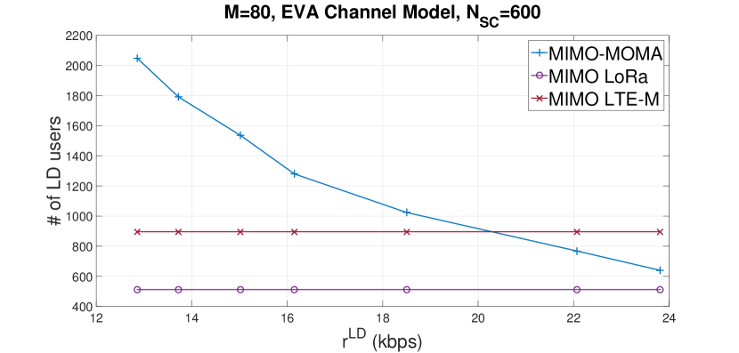
Figure 2: Number of served LD users within one OFDM symbol vs. the LD data rate requirement. $M=80$ with spatial multiplexing.

It is worth mentioning that the maximum number of simultaneous M2M transmissions in LoRa was computed assuming both a spatial multiplexing gain of 8 (for fair comparison with our MIMO-MOMA setting) and the availability of 16 125kHz-channels, each of which can support up to 7 concurrent transmissions thanks to the multiplexing capabilities of chirp spread spectrum [6].

Finally, Fig. 3 shows that MIMO-MOMA achieves HD data rates that are very close to the maximum value achievable with perfect orthogonality. For instance, the HD data rate achieved by MOMA on EPA channels (resp. on EVA channels) with single-user detection stays withing 99% (resp. within 86%) of the perfect-orthogonality upper bound. Note that this performance is achieved by MOMA while serving a number of concurrent LD transmissions as large as 4 times the number that can be supported with narrow-band cellular IoT solutions.

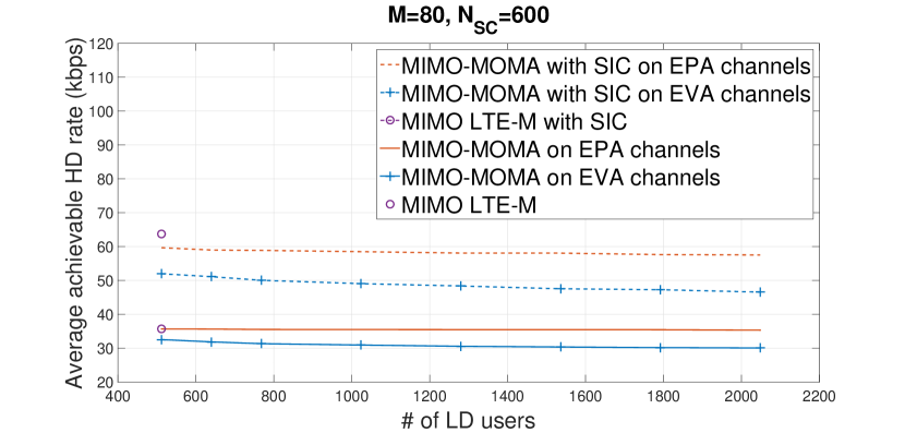
Figure 3: Achievable rate of HD users vs. the number of served LD users within one OFDM symbol. $M=80$ with spatial multiplexing.

VI Conclusion

In this article, we presented a novel multiple access scheme (MOMA) for next-generation cellular networks that is fully compatible with massive MIMO. This scheme is based on assigning, in a flexible and dynamic manner, different resources and different degrees of resource overloading to different classes of users, each representing a different data rate requirement and/or a different service type. Moreover, transmissions from different classes in MOMA are quasi-orthogonal. This way, the use of non-orthogonal access for the lower-rate classes would only slightly affect the broadband users, dropping the need for wasteful guard bands, for subband-based filtering or for complex receiver schemes.

References

• [1] M. Centenaro, L. Vangelista, A. Zanella, and M. Zorzi, Long-Range Communications in Unlicensed Bands: the Rising Stars in the IoT and Smart City Scenarios. Available: http://arXiv:1510.00620v1, Oct. 2015.
• [2] The 3rd Generation Partnership Project (3GPP), 3GPP Technical Specifications 22.368, V.13.0.0, Service Requirements for Machine-Type Communications (MTC); Stage 1. Available: http://www.3gpp.org/, Dec. 2014.
• [3] NGMN, NGMN 5G White Paper. Available: http://www.ngmn.org/, March 2015.
• [4] Nokia Networks, LTE-M - Optimizing LTE for the Internet of Things. Available: http://networks.nokia.com/, 2014.
• [5] J. Abdoli, M. Jia, and J. Ma, Filtered OFDM: A New Waveform for Future Wireless Systems, in SPAWC, Stockholm, July 2015.
• [6] LoRa${}^{\textrm{TM}}$ Alliance, “LoRa${}^{\textrm{TM}}$ Specifications V1.0,” Tech. Rep., May 2015.
• [7] G. Naddafzadeh-Shirazi, L. Lampe, G. Vos, and S. Bennett, “Coverage Enhancement Techniques for Machine-to-Machine Communications over LTE,” IEEE Communications Magazine, vol. 53, no. 7, July 2015.
• [8] J. Korhonen, Introduction to 3G Mobile Communications, 2nd ed. Artech House, Norwood, MA, USA, 2003.
• [9] S. V. Hanly and D. Tse, “Resource Pooling and Effective Bandwidths in CDMA Networks with Multiuser Receivers and Spatial Diversity,” IEEE Trans. Inf. Theory, vol. 47, no. 4, May 2001, pp. 1328-1351.
• [10] E. Björnson, E. G. Larsson, and T. L. Marzetta, Massive MIMO: Ten Myths and One Critical Question. Avilable: http://arXiv:1503.06854v2, Aug. 2015.
• [11] D. Tse and S. V. Hanly, “Linear Multiuser receivers: Effective Interference, Effective Bandwidth and User Capacity,” IEEE Trans. Inf. Theory, vol. 45, no. 2, May 1999, pp. 641-657.
• [12] The 3rd Generation Partnership Project (3GPP), Evolved Universal Terrestrial Radio Access (E-UTRA); Base Station (BS) Radio Transmission and Reception. Available: http://www.3gpp.org/, Sept. 2015.
• [13] V.S. Abhayawardhana, I.J. Wassell, D. Crosby, M.P. Sellars, and M.G. Brown, Comparison of Empirical Propagation Path Loss Models for Fixed Wireless Access Systems, in VTC Spring, Stockholm, May 2005, pp. 73-77 .