X-ray, UV and optical analysis of supergiants: $\epsilon$ Ori

Abstract

We present a multi-wavelength (X-ray to optical) analysis, based on non-local thermodynamic equilibrium photospheric+wind models, of the B0 Ia-supergiant: $\epsilon$ Ori. The aim is to test the consistency of physical parameters, such as the mass-loss rate and CNO abundances, derived from different spectral bands. The derived mass-loss rate is $\hbox{$\dot{\rm M}$}/\sqrt{f_{\infty}}\sim$1.6$\times$10^-6 M_⊙ yr^-1 where $f_{\infty}$ is the volume filling factor. However, the S iv $\lambda\lambda$1062,1073 profiles are too strong in the models; to fit the observed profiles it is necessary to use $f_{\infty}<$0.01. This value is a factor of 5 to 10 lower than inferred from other diagnostics, and implies $\hbox{$\dot{\rm M}$}\lesssim 1\times 10^{-7}$ M_⊙ yr^-1. The discrepancy could be related to porosity-vorosity effects or a problem with the ionization of sulfur in the wind. To fit the UV profiles of N v and O vi it was necessary to include emission from an interclump medium with a density contrast ($\rho_{cl}/\rho_{ICM}$) of $\sim$100. X-ray emission in H-He like and Fe L lines was modeled using four plasma components located within the wind. We derive plasma temperatures from $1\times 10^{6}$ to $7\times 10^{6}$ K, with lower temperatures starting in the outer regions (R${}_{0}\sim$3-6 R_∗), and a hot component starting closer to the star (R${}_{0}\lesssim$2.9 R_∗). From X-ray line profiles we infer $\hbox{$\dot{\rm M}$}<\,$4.9$\times$10^-7  M_⊙ yr^-1. The X-ray spectrum ($\geq$0.1 kev) yields an X-ray luminosity $L_{\rm X}\sim 2.0\times 10^{-7}L_{\rm bol}$, consistent with the superion line profiles. X-ray abundances are in agreement with those derived from the UV and optical analysis: $\epsilon$ Ori is slightly enhanced in nitrogen and depleted in carbon and oxygen, evidence for CNO processed material.

1 INTRODUCTION

Massive stars play a fundamental role in the Universe. Considered the progenitors of core collapse supernovae, they are also responsible for galactic H ii regions, the transfer of mass, momentum and energy to the interstellar medium (ISM), and for metal enrichment in their host galaxy.

Among the stellar wind properties, the mass-loss rate ($\dot{\rm M}$) is crucial for understanding the evolution of massive stars. $\dot{\rm M}$ affects the star’s lifetime on the main sequence, the rotation rate of the star, and the star’s subsequent evolution (e.g. Chiosi & Maeder, 1986; Maeder & Meynet, 2000). The first estimates for $\dot{\rm M}$ were derived assuming spherical smooth winds. However, subsequent observations reveal inconsistencies. For instance, the far UV resonance line profiles (e.g. P v and S iv) observed by COPERNICUS and FUSE cannot be simultaneously fit with H$\alpha$ (e.g. Crowther et al., 2002; Hillier, 2003). Futhermore, P Cygni profiles from highly ionized species, such as N v and O vi, were detected in the UV spectrum (Snow & Morton, 1976), but such ionization states are incompatible with radiative equilibrium in a smooth wind. Cassinelli & Olson (1979) suggested that these ions could be produced by Auger ionization by X-rays (double ionization due to ejection of an inner shell electron by a X-Ray photon.), a suggestion confirmed by Einstein X-ray Observatory which found that massive stars are strong X-ray sources (Harnden et al., 1979; Seward et al., 1979). Two scenarios were proposed to explain the observed X-ray emission: emission from a corona just above the photosphere (Hearn, 1975; Cassinelli & Olson, 1979) and X-ray emission from shock-heated plasma distributed throughout the wind (Lucy & White, 1980; Lucy, 1982; Owocki et al., 1988). The latter is now generally accepted as the dominant X-ray emission mechanism in single stars.

Because of the deficiencies discussed above, the “standard” smooth wind model needed to be revised. At present, it is widely accepted that the winds of massive stars are strongly structured (clumped). The existence of such winds is supported by hydrodynamical time-dependent simulations that predict that radiation-driven winds are unstable (Owocki et al., 1988; Feldmeier et al., 1997; Runacres & Owocki, 2002). Evidence for these inhomogeneities has been found, for instance, by observations of variable discrete absorption components (DAC) in UV and optical lines (e.g. Fullerton et al., 1996; Kaper et al., 1996; Morel et al., 2004; Prinja et al., 2006), and from observations of stochastic variability (e.g., Eversberg et al., 1998). Hillier (1991) showed that the electron scattering wings of recombination lines of Wolf-Rayet (W-R) stars cannot be reproduced by smooth winds, necessitating clumped models and lower mass-loss rates to fit them.

Clumping can be treated using two approximations. The simplest approach considers optically thin clumps at all wavelengths (“microclumping”). The second approach allows for the optical thickness of clumps, especially for lines (“macroclumping”). Commonly it is assumed that the interclump medium is void. However, recently it has been shown that its influence is not negligible (e.g. Zsargó et al., 2008).

Microclumping has been used to lower the discrepancy between P v UV resonance lines and H$\alpha$. Typical filling factors in O stars are 0.01 to 0.1, although, in some cases, it still may be necessary to reduce the P abundance by a factor of 2 from the expected value (e.g. Crowther et al., 2002; Hillier, 2003; Bouret et al., 2005; Fullerton et al., 2006; Bouret et al., 2012). The principal consequence of microclumping is a reduction of mass-loss rates by factors from 3 to 10.

A 3D Monte-Carlo simulation performed by Šurlan et al. (2013) showed that when macroclumping is included the H$\alpha$ and P v lines discrepancy is fixed for higher values of the volume filling factor, yielding higher mass-loss rates when compared with those based on pure microclumping (see also Oskinova et al., 2007; Sundqvist et al., 2010; Šurlan et al., 2012).

The problem with all these analyses is degeneracy – there are several parameters which can be varied but only a few lines that can be modeled, making it difficult to reach definitive conclusions (see details in Šurlan et al., 2013).

As noted by several different authors (e.g. Cohen et al., 2010), the fitting of X-ray lines provides an independent method to estimate the mass-loss rates of OB stars. Cohen et al. (2010) estimated the characteristic optical depth for X-rays ($\tau_{*}=\kappa\dot{M}/4\pi R_{*}v_{\infty}$), fitting separately X-ray lines and then fitting the best optical depth wavelength distribution using the mass-loss rate as a free parameter. The main reported problem with X-ray line emission is that most of the observed profiles are fairly symmetric. This contradicts models that predict lines skewed to the blue (Macfarlane et al., 1991; Owocki & Cohen, 2001). Three explanations are currently proposed: resonance scattering, lower mass-loss rates and porosity (see Oskinova et al. (2011) for a summary of X-ray emission properties of OB stars). However, resonance scattering cannot explain all observed line profiles (Ignace & Gayley, 2002; Leutenegger et al., 2007), while the needed reduction in the mass-loss rates inferred from H$\alpha$ is large (factors of 2 to 10) (e.g. Cohen et al., 2014a). It has also been argued that the porosity lengths (a measure of mean free path of photons between clumps) required to get symmetric lines are unlikely to be as large as needed (Owocki & Cohen, 2006). Sundqvist et al. (2012) and Leutenegger et al. (2013) concluded that a porosity consistent with the observed X-ray line profiles cannot affect the mass-loss rate determination significantly. Furthermore, Hervé et al. (2013) showed that porosity is not important to explain the X-ray spectrum of $\zeta$ Pup.

With the aim of providing more rigorous constraints, and reducing systematic errors, we present our work on a multi-wavelength analysis of the supergiant $\epsilon$ Ori. The analysis is based on X-ray data from Chandra and XMM-Newton, UV data from IUE, HST, and the COPERNICUS satellite, and optical data taken from POLARBASE archive. The photospheric, wind and hot-plasma parameters are obtained from a modified version of cmfgen (Hillier & Miller, 1998), and the consistency of the derived parameters is examined.

The paper is constructed as follows: In the next section, we present results from previous analyses of $\epsilon$ Ori and its main spectral features. Observational data are described in Section 3 while the method and model assumptions are presented in Section 4. The results of optical, UV and X-ray analysis are given in Section 5. A discussion of the results and conclusions are provided in Sections 6 and 7.

2 $\epsilon$ Ori (HD 37128)

The B0 Ia supergiant star $\epsilon$ Ori (HD 37128) is the central star of the Orion Belt, and is also known as Alnilam (an Arabic word that means “string of pearls” (Knobel, 1909)) and belongs to the Orion OB1(b1) association.

The first attempts to derive the physical parameters for $\epsilon$ Ori using photospheric models in non-local thermodynamic equilibrium (NLTE) were made by Auer & Mihalas (1972) and Lamers (1974) who used optical line profiles, and found an effective temperature around 29000 K and $\log g$=3.0. McErlean et al. (1998) using an NLTE model found similar parameters, while Kudritzki et al. (1999), using the original version of the code fastwind (Santolaya-Rey et al., 1997; Puls et al., 2005) found T_eff=28000 K and $\log g$=3.0.

Crowther et al. (2006) and Searle et al. (2008) used the NLTE transfer code cmfgen (Hillier & Miller, 1998) to derive effective temperatures of 27000 K and 27500 K respectively. However, there exists a discrepancy between their $\log g$ values – Crowther et al. reported a value of 2.9 while Searle et al. reported 3.1. Both works also analyzed the CNO abundances of $\epsilon$ Ori. In contrast to the nitrogen deficiency reported by Walborn (1976), Crowther et al. reported a slight enrichment of nitrogen and depletion of carbon. On the other hand, Searle et al. found a nitrogen and carbon deficiency and a solar oxygen abundance.

Previous values for mass-loss rate from different diagnostics encompass values from 1.5$\times$10^-6 to 4.3$\times$10^-6  M_⊙ yr^-1. Diagnostics include H$\alpha$ strength (Kudritzki et al., 1999; Crowther et al., 2006; Searle et al., 2008; Urbaneja, 2004), UV P Cyg profiles (Howarth & Lamers, 1999), thermal radio fluxes (Blomme et al., 2002; Lamers & Leitherer, 1993) as well as H and He infrared lines in the H and K bands (Repolust et al. 2005; they derived an upper limit of $\dot{\rm M}$=5.25$\times$10^-6  M_⊙ yr^-1). These values where derived using smooth winds. In a subsequent analysis by Najarro et al. (2011), lines from the L band were used in conjunction with UV and optical data to obtain a mass-loss rate of $\dot{\rm M}/\sqrt{f_{\infty}}$=2.65$\times$10^-6  M_⊙ yr^-1 and a filling factor $f_{\infty}$=0.03.

Mass-loss rate determinations should all be scaled to the same distance, since the mass-loss rate typically scales as $d^{1.5}$ for $\rho^{2}$ dependent diagnostics (or $d$ for $\rho$ dependent diagnostics such as X-ray profiles). Distance estimates for $\epsilon$ Ori tend to cluster around 400 pc (Lesh, 1968; Lamers, 1974; Savage et al., 1977; Brown et al., 1994), and are broadly consistent with the initial HIPPARCOS determination of 412 pc (Perryman et al., 1997). However, with the latest calibration the new estimate is 606 pc (van Leeuwen, 2007). This distance is the highest ever estimated, and substantially increases the luminosity and mass-loss rate for $\epsilon$ Ori.

IUE and COPERNICUS spectra of $\epsilon$ Ori show line emission from N v and O vi resonance transitions, which, given the effective temperature of $\epsilon$ Ori, provides evidence of X-ray emission in wind. Chandra and XMM spectra of HD 37128 show strong emission lines from H/He-like atoms of C, N, O, Ne, Mg and Si as well as Fe xvii lines.

Previous analyses of X-ray emission from $\epsilon$ Ori found a wide spatial distribution of the hot plasma in the wind. Cohen et al. (2014a) fitted Chandra lines and did not find any correlation between the onset radius for emitting plasma and the emitting ion. This confirmed the results by Leutenegger et al. (2006) who found no evidence for different spatial distributions for different ions.

Recently, Cohen et al. (2014a) estimated the mass-loss rate for $\epsilon$ Ori by fitting X-ray line profiles. They reported two values of mass-loss rate: 2.1$\times$10^-7  M_⊙ yr^-1 and 6.5$\times$10^-7  M_⊙ yr^-1. The first value uses nine X-ray lines while the second value excludes three lines that might be influenced by resonance scattering.

$\epsilon$ Ori shows spectral variability in both the optical and UV. The main variability detected in the UV is associated with DACs, especially in the blue wing of the Si iv and N v doublets. Some other UV lines, including string photospheric lines, also show variability (Prinja et al., 2002). In the optical H$\alpha$ shows strong variability with changes in both shape and strength occurring on a time scales of hours to tens of days (e.g. Ebbets, 1982; Morel et al., 2004; Prinja et al., 2004; Thompson & Morrison, 2013, and references therein). One possible cause of the variability is radial and non-radial oscillations that produce a mass-loss rate modulation (Thompson & Morrison, 2013). Our calculations show that variations of $\pm 30\%$ in $\dot{\rm M}$ about our derived value can explain the observed variations of H$\alpha$.

We chose $\epsilon$ Ori as a standard early B supergiant due to the availability of high resolution X-Ray, UV and optical data. In practice, spectral variability is common is B supergiants, and hence unavoidable. Its variability will introduce uncertainties in the derived wind parameters, but these uncertainties can be qualified, and will not affect our main aim of evaluating the consistency of the main physical parameters of $\epsilon$ Ori derived in this multi-wavelength analysis.

3 THE DATA

For this work we collected optical, UV and X-ray data from different archives as described below. The sources of the data is presented in Table 1.

3.1 Optical Data

The optical data were obtained from POLARBASE, the stellar spectra archive for the NARVAL and ESPaDOns echelle spectropolarimeters. The former is installed in the Télescope Bernard Lyot (TBL, Pic du Midi Observatory) and the latter at the Canada-French-Hawaii Telescope. A detailed description of these instruments can be found in Silvester et al. (2012) and Petit et al. (2014). They are twin spectropolarimeters except for the aperture (2.8 arcsec for NARVAL and 1.6 arcsec for ESPaDOns). Both of them have a spectral resolution R=$\lambda/\Delta\lambda$ $\simeq$ 65000 and a spectral coverage from 3690 to 10000 Å. The wavelength calibration is performed using a Th-Ar spectra and it is refined using telluric bands as references for radial velocity. The instruments have two modes of operation: spectroscopic and polarimetric. In the polarimetric mode, the beam is split with a Wolloston prism, and the new beams are then conducted to a spectrometer through fibers. The $I$ Stokes parameter is obtained by adding these two spectra; the rest of the Stokes parameters (V, Q and U) are extracted by combinations as described by Bagnulo et al. (2009)(see also Petit et al., 2014).

The early B supergiant star $\epsilon$ Ori has been observed by both of these instruments at different epochs. Because of its spectral variability we selected for this work one set of 112 exposures taken by NARVAL on October 19th, 2007 during 4 hours (universal time from archive) in polarimetric mode. Every exposure has a signal to noise ratio of $\sim$ 600. The reduction for each of these exposures was automatically performed by the Libre-Esprit reduction pipeline (Petit et al., 2014). We chose the “$I$” Stokes spectra from the archive for this work. All of the exposures were combined and the resulting spectrum normalized using soft spline functions between nodes chosen by visual exploration to avoid spurious oscillations. This task was performed through the line_norm procedure from FUSE IDL tools This combined and normalized spectrum was used for the analysis.

Table 1: Summary of data of $\epsilon$ Ori: optical (NARVAL), ultraviolet (IUE, HST and COPERNICUS) and X-ray (Chandra and XMM-Newton).

ID Obs.	Date	Julian Date	Spectral Range (Å)	$\lambda/\Delta\lambda$
NARVAL (Optical)
–	Oct-19-2007	2454392.55907	3690 - 10000	65000
IUE (UV)
SWP30177	Jan-28-1987	2446823.57668	1150-1975	10000
SWP30196	Jan-30-1987	2446825.56254	1150-1975	10000
SWP30204	Jan-31-1987	2446826.54533	1150-1975	10000
SWP30216	Feb-01-1987	2446827.57926	1150-1975	10000
SWP30225	Feb-01-1987	2446828.47190	1150-1975	10000
SWP30242	Feb-03-1987	2446829.64887	1150-1975	10000
SWP30249	Feb-03-1987	2446830.47746	1150-1975	10000
SWP30257	Feb-05-1987	2446831.64990	1150-1975	10000
SWP30266	Feb-06-1987	2446832.66278	1150-1975	10000
SWP30272	Feb-06-1987	2446833.47835	1150-1975	10000
LWR02238	Sep-01-1978	2443753.35590	1900-3080	14000
LWR02239	Sep-01-1978	2443753.40463	1900-3080	14000
LWR02240	Sep-01-1978	2443753.42454	1900-3080	14000
GHRS (UV)
Z1BW040TT	Nov-11-1994	2449302.5975	1180-1218	20000
Z1BW040UT	Nov-11-1994	2449302.5000	1229-1268	20000
Z1BW040VT	Nov-11-1994	2449302.5019	1273-1311	20000
Z1BW040WT	Nov-11-1994	2449302.5389	1324-1363	20000
Z1BW040XT	Nov-11-1994	2449302.5408	1385-1423	20000
Z1BW040YT	Nov-11-1994	2449302.5428	1527-1564	20000
Z1BW040ZT	Nov-11-1994	2449302.5634	1588-1625	20000
Z1BW0400T	Nov-11-1994	2449302.5656	1649-1684	20000
COPERNICUS (UV)
027	Nov-30-1972	2441652.49738	1000-1420	5500
Chandra (X-ray)
3753	Dec-12-2003	2452986.00475	2-26	150-1100
XMM-Newton (X-ray)
0112400101	Mar-06-2002	2452339.84921	5-35	150-800

3.2 UV Data

3.2.1 IUE

The International Ultraviolet Explorer (IUE) has observed $\epsilon$ Ori in both low and high dispersion modes. For this work, we selected data obtained for the BSIGP program (PI: Geraldine Peters) from the MAST archive. These 10 exposures of $\epsilon$ Ori were undertaken from January 28th, 1987 to February 6th, 1987 in high dispersion and utilizing the large aperture with the short-wavelength prime camera (SWP). This instrumental configuration yields a spectral resolution of $\lambda/\Delta\lambda$ $\sim$10000 with a spectral coverage of $\lambda\lambda$1150-1975. When extracted, the spectra did not show strong variability, so we combined them to obtain the final mean spectrum.

The IUE observation program HSCAD (PI: A.K. Dupree) has 33 exposures of $\epsilon$ Ori taken through the small aperture. When combined and scaled to BSIGP fluxes, no significant differences were detected when compared with the higher signal-to-noise BSIGP observations.

For long-wavelength we averaged the three exposures made on January 9th, 1979 using the LWR camera (1900-3080 Å) at high dispersion ($\lambda/\Delta\lambda$ $\sim$14000) and small aperture. This data were collected within the program ID: UK022 (PI: P. Byrne).

3.2.2 GHRS/HST

Hubble Space Telescope (HST) observed $\epsilon$ Ori only with the Goddard High Resolution Spectrograph (GHRS) (programs: 3472, 6070 6541, 3859 and 6249). As the programs focused on interstellar abundances using specific diagnostic lines, none of the observations covered a wide spectral range. We used the observations from program 3472 (PI: Lewis Hobbs), that were collected on November 11th, 1994. We retrieved the calibrated data from the G160M first-order grating at intermediate resolution (R$\simeq$25000) from the MAST archive. We treated the data using the STSDAS package and related tasks from analysis software IRAF.

Table 2: Species and ions included in cmfgen models. F is the number of levels for each atomic model and S denotes the super-levels used in calculations. “E\I” denotes Element\Ionization.

E\I	I			II			III			IV			V			VI			VII
	F	S		F	S		F	S		F	S		F	S		F	S		F	S
H	30	20
He	69	45		30	22
C				92	40		84	51		64	64
N				85	45		82	41		76	44		49	41
O				123	54		170	88		78	38		56	32
Ne							71	28		52	17		166	37
Si				100	72		33	33		33	22
P										90	30		62	16
S							44	24		142	51		98	31
Fe							1433	104		520	74		220	50		433	44		153	29

3.2.3 Copernicus

Copernicus observations of $\epsilon$ Ori (star: 027) were also retrieved from the MAST archive. We selected scans that covered a large spectral range, and that included O vi $\lambda$1032,1038, S iv $\lambda$1062,1073 and P v $\lambda$1118,1028. We co-added those scans and generated the spectrum using the IDL IUEDAC library tools and normalized it using soft spline functions between selected nodes in the same sense as explained above for the optical data. After selecting, co-adding and normalizing, we obtained a spectrum with coverage of $\lambda\lambda$1000-1450.

3.3 X-ray Data

3.3.1 Chandra

Chandra observed $\epsilon$ Ori on December, 12^th 2003, using the gratings of HETGS (High Energy Transition Grating Spectrometer) for 92 ks (PI: Wayne Waldron). The FWHM spectral resolutions are 23 mÅ and 12 mÅ for Medium Energy Grating (MEG) and High Energy Grating (HEG) respectively. The effective area of these gratings is significant for $\lambda\gtrsim$2 Å but falls strongly beyond $\lambda\gtrsim$ 16 Å in the case of HEG and $\lambda\gtrsim$ 25 Å for MEG. Because of the small number of counts collected in the HEG, we only used MEG data for this work. We reprocessed the data using the CIAO version 4.6 tasks, following the standard threads as described in the CIAO documentation. We combined the positive and negative first order MEG spectra using add_grating_orders task.

3.3.2 XMM-Newton

XMM-Newton observed $\epsilon$ Ori on 6th March, 2002 using the instruments: EPIC-MOS(1,2), EPIC-pn and the Reflection Grating Spectrometers (RGS1 and RGS2) (PI: Martin Turner). Our analysis was based only on the RGS data due to its high spectral resolution (R$\sim$250 at 15 Å). The exposure time for both spectrometers was 13 ks.

The data were reduced following standard procedures with SAS v13.5.0. We use the first order spectra of each spectrometer (RGS1 and RGS2) for the analysis. Together, RGS1 and RGS2 have a spectral coverage from 6 to 39 Å.

4 THE METHOD

The analysis was undertaken in two main stages. In the first stage we derived the photospheric and wind parameters using the standard method for massive stars and the latest version of cmfgen. In the second stage, the X-ray emission is modeled. We then tested the consistency of the adopted parameters with the X-ray line profiles (mass-loss rates) and line ratios (abundances).

4.1 Modeling Assumptions

4.1.1 Optical and UV analysis

The calculations for our analysis were performed using the code cmfgen (Hillier & Miller, 1998). This code models a spherical stellar atmosphere and stellar wind solving the radiative transfer, radiative and statistical equilibrium equation system in non-LTE (NLTE) taking into account line-blanketing effects. The transfer equation is solved in the co-moving frame (CMF). Table 2 describes the ionization states and number of full atomic levels and super-levels for each atomic species included in the models.

The photospheric density structure is calculated by iteratively solving the hydrostatic equilibrium equation system below the sonic point as described by Bouret et al. (2012). Given an adopted mass-loss rate and the velocity profile $v(r)$, the wind density structure is calculated using the continuity equation. The adopted velocity profile is similar to that commonly used for massive star winds (e.g. Hillier, 2003):

$$v(r)=\frac{2v_{tr}+(v_{\infty}-2v_{tr})(1-r_{tr}/r)^{\beta}}{1+\exp{[(r_{tr}-r})/h_{eff}]},$$ (1)

where $v_{tr}$ and $r_{tr}$ are the transition velocity and radius, between the photosphere and wind. The transition point is set as the radius where $v(r_{tr})=0.75v_{s}$ where $v_{s}{\sim}15$  km s^-1 is the sound velocity. The term $h_{eff}=v_{tr}/(2(dv/dr)_{tr})$, is the scale height, $v_{\infty}$ is the terminal velocity and $\beta$ is the acceleration parameter.

Clumping is taken into account through the volume filling factor $f=\bar{\rho}/\rho(r)$, where $\bar{\rho}$ is the homogeneous (unclumped) wind density and $\rho$ is the density in clumps. In this approach the clumps are assumed to be optically thin to radiation and the interclump medium is void (Hillier & Miller, 1999). The filling factor dependence with radius is defined by the relation: $f=f_{\infty}+(1-f_{\infty})\exp(-v(r)/v_{cl})$, where $v_{cl}$ characterizes the velocity where clumping starts.

It is well known that we need to include the effect of microturbulence on the photospheric and wind spectrum (e.g. Howarth et al., 1997). For the formal solution, the depth dependence of the microturbulence velocity was parameterized as in Hillier (2003): $\xi_{t}=\xi_{min}+(\xi_{max}-\xi_{min})v(r)/v_{\infty}$. Here, $\xi_{min}$ and $\xi_{max}$ are the photospheric and wind turbulence respectively. In this work we varied the $\xi_{min}$ from 10 to 20  km s^-1, a reasonable range for early B supergiant stars (McErlean et al., 1998) and $\xi_{max}\sim$ 0.1-0.3 $v_{\infty}$. In the CMFGEN calculation we used a microturbulent velocity that was independent of depth.

4.1.2 X-ray Analysis

We assume that the X-ray emission comes from an ensemble of shock-heated regions within the wind (shock scenario). The shock scenario predicts regions distributed in the wind where the plasma is strongly heated due to shocks caused by radiative instabilities (Owocki et al., 1988; Feldmeier et al., 1997).

The current version of cmfgen allows for X-ray emission from shocked regions in the wind using emissivity tables from apec (Smith et al., 2001) for different temperatures, but it doesn’t take into account differences in abundances (generally), densities or the influence of the UV radiation on the populations of the levels that give rise to the X-ray lines.

Recently Zsargó et al. (2015, in preparation) developed a new version called xcmfgen that makes possible a consistent interaction between the code apec and cmfgen. Here we will briefly describe the main features of the method to compute the synthetic X-ray spectrum taking into account the wind radiation from cmfgen.

As a convenient approximation, a set of $N_{p}$ plasmas, characterized by their temperature (T_X), the radius where the plasma emission starts (R₀), and the X-ray filling factor ($f_{X}$), are distributed within the wind. The filling factor is parametrized as follows:

$$f_{X-ray}(r)=\begin{cases}f_{X}&\text{if }r\geq R_{0}\\ f_{X}e^{-(v(R_{0})/v(r))^{2}(R_{0}/r)^{4}}&\text{if }r<R_{0},\end{cases}$$ (2)

where $v(r)$ is the wind velocity profile and $f_{X}$ is the filling factor at infinity. An iterative process is then performed to derive the best estimates of the plasma parameters. A xcmfgen run is done to calculate the stellar wind structure. Then, apec is called in order to calculate a grid of plasma emissivities covering the wind densities and plasma temperatures. The relation between the plasma and wind density is set as: $n_{plasma}$=4$n_{wind}$ (adiabatic shock approximation). Here $n_{wind}$ corresponds to the density of the unclumped model. The relation between the plasma and wind density only has a very minor influence on the analysis – it’s primary effect will be in the interpretation of the derived filling factors (e.g. what fraction of the wind is shocked).

The Astrophysical Plasma Emission Code (apec) is a code for calculating level populations and emissivities for a hot plasma in collisional equilibrium. This code uses an extensive library of cross-sections (ATOMDB). In this work we use this library as it is described in Foster et al. (2012). Some changes were implemented in apec in order to read the xcmfgen outputs as well as to use the corresponding abundances. The main change was the inclusion of the radiative excitation (i.e. UV photoexcitation) and deexcitation rates in the statistical equilibrium equations. The UV emission from the wind affects the forbidden to intercombination ratio R=f/i of the He-like triplets (Gabriel & Jordan, 1969; Porquet et al., 2001).

Once apec has calculated the grid of plasma emissivities, a new run of xcmfgen is performed including the emissivities from apec. This process yields a new radiation field that is used in a second apec computation. Usually, it is necessary for only two loops (i.e., xcmfgen - apec - xcmfgen - apec - xcmfgen) to get a consistent model.

A necessary condition to apply this method is that the X-rays do not strongly affect the bulk of the cool wind. As noted previously by Martins et al. (2005) and Macfarlane et al. (1994), this condition holds for early O supergiants. However, for late O and B stars X-rays could change the wind ionization in a non-negligible way. An analysis of that influence in the case of $\epsilon$ Ori is presented in Section 6.3. We conclude that for clumped wind models this effect is low enough to apply this method. Thus, we applied the same fit procedure described by Zsargó et al. (2015, in preparation) in their study of $\zeta$ Pup and did the X-ray analysis separately from the optical and UV analysis.

We created a two-dimensional grid in (T_X,R₀), varying each of them between the following ranges: T_X=1.0-16.0$\times$10⁶ K and R₀=1.2-6.1R_∗. We then used cmf_flux to compute the X-ray spectrum for each (T_X,R₀) combination. The starting filling factor is fixed at $f_{X}$=5$\times$10^-5; the corresponding value for each plasma component is adjusted subsequently as described below.

The total X-ray spectrum results from adding the contributions from each plasma component after it has propagated through the wind. We adjusted the plasma distributions (i.e. number of components, T_X, R₀ and $f_{X}$) using the fitting package xspec (Arnaud, 1996) of HEASARC. A multiplicative model is included to take into account the effect of interstellar absorption on the X-ray spectrum. The column density of neutral H used in this work is $\log[N(\textrm{H\,{\sc i}})]$ cm^-2=20.48 (Diplas & Savage, 1994). As the molecular absorption in the direction of $\epsilon$ Ori is low it doesn’t affect the X-ray spectrum and hence is ignored.

Because of the small number of counts in the Chandra and XMM-Newton observations, Poisson noise dominates, and we use the C-statistic (Cash, 1979) to determine the quality of the fits. While an arbitrary number of components can be included, the final models were typically composed of only four different temperatures.

The X-ray lines included in the analyses are listed in Table 3.

Table 3: $\epsilon$ Ori Chandra and XMM-Newton lines. Data from ATOMDB.

Ion	Wavelength (Å)	Type	Tpeak [106 K]
Si xiv	6.1822	H-like	15.8
Si xiii	6.6479, 6.6866, 6.6866	He-like	10.0
Al xii	7.7573, 7.8070, 7.8721	He-like	7.94
Mg xi	7.8503	He-like	6.31
Mg xii	8.4210	H-like	10.0
Mg xi	9.1687, 9.2297, 9.3143	He-like	6.31
Ne x	10.2388	H-like	6.31
Ne ix	11.5440	He-like	3.98
Ne x	12.1339	H-like	6.31
Fe xvii	12.2660	L-shell	6.31
Ne ix	13.4470, 13.5520, 13.6980	He-like	3.98
Fe xvii	14.2080	L-shell	7.94
Fe xvii	15.0140	L-shell	6.31
Fe xvii	15.2610	L-shell	6.31
Fe xvii	16.0040	L-shell	7.94
O viii	16.0060	H-like	3.16
Fe xvii	16.7800	L-shell	6.31
Fe xvii	17.0510	L-shell	6.31
Fe xvii	17.0960	L-shell	6.31
O vii	18.6270	He-like	2.00
O viii	18.9670	H-like	3.16
O vii	21.6020, 21.8040, 22.0980	He-like	2.00
N vii	24.7790	H-like	2.00
N vi	24.8980	He-like	1.59
C vi	26.9900	H-like	1.59
C vi	28.4650	H-like	1.59
N vi	28.7870, 29.0810, 29.5340	He-like	1.58
C vi	33.7370	H-like	1.26

4.2 Stellar Parameters

We used the optical spectrum to estimate the photospheric parameters such as the effective temperature, gravity and surface abundances. The method follows the analysis route described by Bouret et al. (2012) (see also Martins et al., 2005; Bouret et al., 2013). We adopted a radial velocity $v_{r}$=25.9$\pm$0.9  km s^-1 (Evans, 1967).

A brief description of steps taken to derive the fundamental stellar parameters ($T_{eff}$, $\log g$, and CNO, Fe and Si abundances) follows.

4.2.1 Luminosity

We adopt two distances: the distance $d=$411.5${}^{+245}_{-112}$ pc (Perryman et al., 1997) from the old HIPPARCOS catalog (HIP 26311), and $d$=606${}^{+227}_{-130}$ pc (van Leeuwen, 2007) who reanalyzed HIPPARCOS  data. The errors on the distance are approximately 30-50%, which will yield an error on the luminosity of 60-100%, and a similar, but somewhat smaller, uncertainty on the mass-loss rate.

A first estimation of luminosity was made based on $M_{V}$ and the bolometric correction (BC). The last one was taken from the relation between T_eff and BC calculated by Crowther et al. (2006)(Fig. 4). This relation comes from their sample of Galactic B supergiants and from the SMC B supergiants reported by Trundle et al. (2004) and Trundle & Lennon (2005). For this first approach we used the temperature estimated by Crowther et al. for $\epsilon$ Ori, $T_{eff}$=2.7$\times$10⁴ K. The $M_{V}$ value was estimated from the distance values from HIPPARCOS, the apparent visual magnitude $V$=1.69 (Lee, 1968) and the interstellar visual extinction $A_{V}$=3.1 E(B-V), with E(B-V) taken from the Crowther et al. study, E(B-V)=0.06. Thus, $M_{V}$=$-6.57$ for $d$=411.5 pc and $M_{V}$=$-7.41$ for $d$=606.06 pc. The luminosity is given by:

$$\log(L_{*}/L_{\odot})=(M_{B\odot}-M_{V}-BC)/2.5,$$ (3)

where $M_{B\odot}$ is the solar bolometric magnitude ($M_{B\odot}$=4.75).

Once the temperature and gravity were estimated, we used the UV flux, and the optical magnitudes ($UVB$) in order to re-estimate simultaneously the luminosity and E(B-V) values.

4.2.2 Gravity and Effective Temperature

For estimating the effective temperature and gravity ($\log g$) a small grid of models encompassing $T_{eff}$=2.5-2.9$\times$10⁴ K and $\log g=2.8$ to 3.4, with steps of $0.1\times 10^{4}$ K and 0.1 dex respectively, were computed. The gravity was estimated by fitting the wings of H_β, H_γ, H_δ and H_ϵ – the lines were equally weighted for the gravity analysis. Because of the mass loss rate of $\epsilon$ Ori, these Balmer lines are only very weakly influenced by wind emission. In order to reduce the degeneracy between $\log g$ and $T_{eff}$, the equivalent widths for He i and He ii lines were also utilized. The lines used were: He i $\lambda\lambda$4010, 4389, 5049 and He ii $\lambda\lambda$4201, 4542. These lines show a weak dependence on the microturbulence.

For computing the effective temperature we used the ionization balance of both He i to He ii and Si iii to Si iv. We used the same grid described above to fit the Si iv $\lambda$4090, Si iv $\lambda$4115 and Si iii $\lambda$4554-76 lines beside the He i $\lambda\lambda$4471, 4389, 4922 and the He ii lines described above. UV lines, especially those belonging to Fe iv (1550 - 1700 Å), Fe v (1360 - 1385 Å) as well as Fe iii (1800-1950 Å), were used to check the result.

4.2.3 Microturbulence

To estimate the photospheric microturbulent velocity we calculated spectra for three values of $\xi_{min}$ (10, 15 and 20  km s^-1) and fitted the equivalent width of the 4472, 5017 and 6680 Å He i lines, and the Si iii triplet at 4554-4576 Å. Our exploration of synthetic spectra shows that these lines depend strongly on the $\xi_{min}$ value and are weakly influenced by blending or abundance effects.

4.2.4 Surface Abundances

Once the temperature and gravity were constrained, we determined the surface abundances of the main species, namely, He, C, N, O, Si and Fe as follows:

Helium. As pointed out by McErlean et al. (1999, 1998), it is difficult to determine the He abundance in B stars primarily because triplet and singlet lines of He i yield different He abundances. Najarro et al. (2006) showed that some He i singlets are influenced by a strong interaction of the He i resonance transition at $\lambda\lambda$4923,5017 with UV Fe iv lines. This interaction directly affects He i 2p $1$P^o, which influences the strength of optical singlet lines that makes them unreliable diagnostics. Najarro et al. suggest using triplet lines for analysis. Based on these issues we decided to set the He abundance, expressed as $y=N[He]/N[He+H]$, to the solar value $y$=0.091 for every one of our models.

Carbon. In the optical, we used lines of C ii $\lambda\lambda$4267,6578-82, C iii $\lambda\lambda$4070,5696,4648-50 and C iv $\lambda\lambda$5802-12. In the case of C iii $\lambda$4648 and C iii $\lambda$5696, Martins & Hillier (2012) showed that these lines have strong interactions with the UV lines Fe iv $\lambda$538 and C iii $\lambda$538, hence, they need be treated carefully. UV lines were used to check the abundance deduced from optical lines. We mainly used C iii $\lambda$1176. The commonly used line C iv $\lambda$1169 is not detected in UV data, since it is blended with C iii $\lambda$1176. The line C iii $\lambda$1247 is blended with N v $\lambda$1238-42 emission and only the red emission can be used as a diagnostic.

Nitrogen. To estimate the nitrogen abundance we used the blend-free lines N ii $\lambda\lambda$3995, 4042-45, 4238-42, 5002-06, 5677-81, and N iii $\lambda\lambda$4380, 4635. As a consistency check we also examined N ii $\lambda$5046 and N iii $\lambda\lambda$4098, 4512-18, 4643, 4868. The former line is blended with He i $\lambda$5049 while N iii $\lambda$4098 is blended with H_δ. In the UV we used N iii $\lambda\lambda$1183-85 and N iii $\lambda\lambda$1748-52. The N iv $\lambda$1718 line was excluded because it is affected by the wind and N v $\lambda$1240 is X-ray sensitive, and hence not suitable as an abundance diagnostic.

Oxygen. $\epsilon$ Ori shows a variety of O ii and O iii lines — our abundance analysis was based on: O iii $\lambda\lambda$4368, 5594 and O ii $\lambda\lambda$4077, 4134, 4663. Other lines that show abundance dependence are those in the blend O ii-iii $\lambda$4415-18. The UV lines commonly used for abundance diagnostics are O iv $\lambda\lambda$1338-43 and O iii $\lambda\lambda$1150-54 but they show only a weak abundance dependence in the models. O v $\lambda$1371 was not detected in the UV spectra of $\epsilon$ Ori.

Silicon. The silicon abundance was estimated using only Si iii and Si iv lines since Si ii lines were not detected. The triplet Si iii $\lambda\lambda$4552-67-74 and Si iii $\lambda$5738 were useful as well as Si iv $\lambda\lambda$4089, 4116. No UV lines were used for the analysis due to their strong dependence on the wind parameters.

Iron. We only used UV Fe lines for estimating its abundance. The iron features Fe v $\lambda\lambda$1360 - 1385, Fe iv $\lambda\lambda$1550 - 1700, and Fe iii $\lambda$1800-1950 were used. Again, it is important to have a reliable value for temperature to get an accurate abundance estimation.

4.2.5 Rotation and Macroturbulence

We account for the influence of rotation on the stellar spectrum in two ways. First, we convolve a rotational broadening profile with the synthetic spectrum. This method assumes solid rotation of both the star and wind, and that the line profile does not vary from the center to the limb (Gray, 2008). Wind-free line profiles were used to estimate the projected rotation velocity ($v_{rot}\sin i$).

In the second technique we calculate the synthetic spectrum using the 2D code developed by Busche & Hillier (2005). This code computes the radiative transfer through the photosphere and wind using an axysimmetric geometry and allows for rotation of the star. Recently, Hillier et al. (2012) studied the application of the code to optical line profiles of O stars. They showed that while the convolution method that is commonly used to allow for rotation is adequate for photospheric absorption lines it fails for lines influenced by photospheric emission, or for lines with wind emission contribution. For the diagnostic lines H$\alpha$ and He ii $\lambda 4686$ it is important that the influence of rotation be correctly modeled.

Because the rotation rate of $\epsilon$ Ori is low we can use the same simplifications as Hillier et al. (2012) – we assume the rotation does not affect the density structure, temperature and surface gravity. We also assume that the star rotates as a solid body below $v(r)$=20  km s^-1 and the angular momentum about the center is conserved above that value.

Finally, in order to compare the synthetic spectra with the optical observational data, it is necessary to take into account instrumental broadening and macroturbulence. Instrumental broadening was taken into account by convolving a Gaussian profile of 4.0  km s^-1 from NARVAL spectral resolution. Macroturbulence broadening was included through a convolution assuming an isotropic Gaussian distributed velocity field. The value of the FWMH of such a distribution in  km s^-1 was estimated using the wings of isolated wind-free metallic lines.

4.3 Wind Parameters

The parameters that describe the stellar wind are those that have to do with the wind velocity law ($\beta$ and $v_{\infty}$), the mass-loss rate ($\dot{\rm M}$), the filling factor ($f_{\infty}$, $v_{cl}$) and the wind turbulent velocity ($\xi_{max}$). All of these influence spectral features in the UV, optical, and X-ray band. Some line profiles are strongly influenced by two or more of the parameters. For example, the strength of H$\alpha$ is highly sensitive to both the mass-loss rate and filling factor, and its profile shape is sensitive to $\beta$. Thus, these wind parameters need to be determined simultaneously using several spectral features from different ions and species.

The value of $\dot{\rm M}$ is first constrained using the H$\alpha$ strength for $f_{\infty}$= 1.0, 0.1, 0.05 and 0.01 ($f_{\infty}$=1.0 means smooth wind). A consistency check was then done using the UV line profiles of C iv $\lambda\lambda$1548,1551, N v $\lambda$1240, Si iv $\lambda\lambda$1394,1403 and C iii $\lambda 1776$, which showed only a weak dependence on mass-loss rate (in our models) when compared with H$\alpha$.

The clumping factor ($f_{\infty}$) is determined using S iv $\lambda\lambda$1062,1073, P v $\lambda\lambda$1118-28 and N iv $\lambda$1718. The parameter $v_{cl}$ has a slight influence on the H$\alpha$ shape, so its value is adjusted only to improve the line profile once the Ṁ is estimated from line strength. Hillier (2003) suggested that its value should be less than 100  km s^-1. Likewise, Bouret et al. (2003) (see also Bouret et al., 2005) suggested that clumping should start close to the photosphere ($v_{cl}\sim$30  km s^-1). For the models in this work, we used $v_{cl}$ values from 20 to 100  km s^-1.

The velocity profile parameters ($v_{\infty}$, $\beta$) were constrained using UV P Cygni line profiles and the H$\alpha$ line profile. The H$\alpha$ profile shape is strongly sensitive to $\beta$ – we used values from 1.0 to 2.4 to find the best profile. Once we alter $\beta$ it is necessary to re-tune the mass-loss rate to match the H$\alpha$ intensity.

In the same sense, $v_{\infty}$ was estimated using the blue wing of the P Cyg profile of C iv $\lambda\lambda$1548,1551 and the Si iv $\lambda\lambda$1394,1403 profile. As the shape of that wing is also affected by the wind turbulence $\xi_{max}$ we tune $v_{\infty}$ and $\xi_{max}$ simultaneously.

4.4 X-ray – Wind Parameters

As X-rays propagate through the wind they can be absorbed at the same time photoionize the gas. The effect on an X-ray line is an attenuation of the profile on the red side, because the red-shifted photons from the rear hemisphere encounter a longer path length through the wind than the blue-shifted photons from the front hemisphere (Owocki & Cohen, 2001; Macfarlane et al., 1991). Since the X-ray opacity varies with wavelength the influence on line profiles varies with wavelength. Furthermore, the strength of the effect depends primarily on the wind column density and hence the mass-loss rate. Thus, with a known opacity distribution, it is possible to estimate the mass-loss rate from the observed X-ray lines (Cohen et al., 2014a).

In this work we utilize X-ray cross-sections from Verner & Yakovlev (1995). The spatial variation in opacity is determined by the velocity law and mass-loss rate. We use the same values estimated from the optical and UV data. Once the best fit is attained, the line profiles are checked for consistency. Previous Ṁ estimations from X-ray lines used individual line profiles (Oskinova et al., 2006; Cohen et al., 2014a); in this work we use models for the whole X-ray spectrum. A similar approximation was developed by Hervé et al. (2013), but they used a fiducial radial dependence for opacity.

The effects of $v_{\infty}$ and $\beta$ on X-ray profiles have been studied by Cohen et al. (2010). Here, we use the same values obtained from the optical and UV analysis. We show below that $\beta$ can influence R₀, and this gives us the opportunity to check our results against the instability wind models (Feldmeier et al., 1997; Runacres & Owocki, 2002; Dessart & Owocki, 2003, 2005) relating the wind acceleration with the shock formation region.

4.5 X-ray – Abundances

Once global best fit to the X-ray spectra is obtained, the abundances are adjusted so as to improve the fit of line ratios.

To compute the observed line strength ratios, the line fluxes were measured using Gaussian profiles and the statistical tools from xspec. The free parameters for each fit were the normalization factor and the line width ($\sigma$ of each Gaussian). The line center is generally fixed at its laboratory value, but when necessary it was shifted to match the peak of the observed line – it was not included as a free parameter in the fit. We will specifically focus on the CNO line ratios. Recently Zsargó et al. (in preparation) showed that good choices are:

$$R(N/O)=\frac{Flux(\mbox{N\,{\sc vii} }Ly\alpha)}{[Flux(\mbox{O\,{\sc viii} }Ly\alpha)+Flux(\mbox{O\,{\sc vii} }He-Like)]},$$ (4)

and

$$R(C/N)=\frac{Flux(\mbox{C\,{\sc vi} }Ly\alpha)}{[Flux(\mbox{N\,{\sc vii} }Ly\alpha)+Flux(\mbox{N\,{\sc vi} }He-Like)]},$$ (5)

that have a weak dependence on temperature and are good choices to test the consistency of our abundance values from the optical and UV analysis. New abundances can be estimated when the observed ratios are compared with the ones from our models.

Table 4: Stellar parameters of $\epsilon$ Ori from optical and UV data.

Log (L∗/L⊙)d	Teff	$\log g$	R∗	M∗	$\xi_{min}$	$v\sin i$	$v_{macro}$	E(B-V)	d
	103 [K]		R⊙	M⊙	km s-1	km s-1	km s-1	mag	pc
5.59${}^{+0.51}_{-0.20}$	27.0$\pm$0.5	3.0$\pm$0.05	28.6	30.0	15-20	40-70c	70-100	0.091 $\pm$ 0.01	412a
5.92${}^{+0.32}_{-0.18}$	27.0$\pm$0.5	3.0$\pm$0.05	42.0	64.5	15-20	40-70c	70-100	0.091 $\pm$ 0.01	606b

• HIPPARCOS catalog (Perryman et al., 1997)

• HIPPARCOS catalog (van Leeuwen, 2007)

• Value computed using the convolution method.

• Errors from distance uncertainties.

5 RESULTS

5.1 Stellar Parameters

The main stellar parameters that we estimated for $\epsilon$ Ori are shown in Table 4. Each row in the table corresponds to the parameters from the two different distances from the HIPPARCOS catalogs. The luminosity from the lower distance lies between those calculated by Crowther et al. (2006) ($\log(L_{*}/L_{\odot})$=5.44) and Searle et al. (2008) ($\log(L_{*}/L_{\odot})$=5.73) and is close to other estimates reported in the literature (e.g. Lamers, 1974; Kudritzki et al., 1999; McErlean et al., 1999). The luminosity computed with the larger distance is the highest value reported and makes $\epsilon$ Ori one of the most luminous B-supergiants in the Galaxy. This value is almost twice the calibrated value found by Searle et al. (2008) for galactic B0Ia stars (They used jointly their sample and that of Crowther et al. (2006).). A similar statement applies to the mass-loss rate and stellar radius (mass). Thus the distance of van Leeuwen (2007) makes $\epsilon$ Ori an unusual B0Ia supergiant. For the analysis, we prefer to use the lower value in order to compare with the previous work on $\epsilon$ Ori that were undertaken assuming a distance closer to that of Perryman et al..

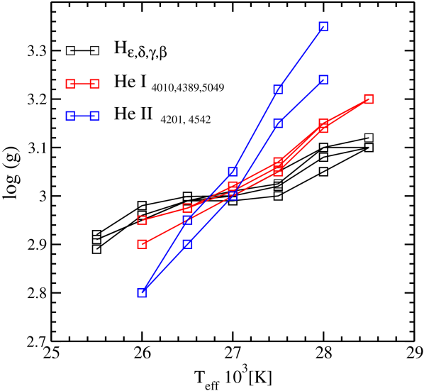
Figure 1: Constraints on $T_{eff}$ and $\log g$. Shown are fits to the Balmer line wings (black), the equivalent width of He i (red) and He ii (blue) lines.

Figure 1 shows the analysis of Balmer line wings and He i-ii lines. We concluded that $\log g$=3.0. We also found that for values greater than 3.05 and lower than 2.95 it is not possible to fit the Balmer and He i-ii lines consistently. Thus, we estimate an error of 0.05 for $\log g$.

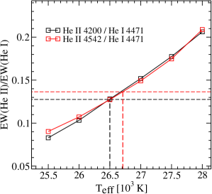
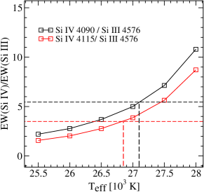
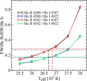
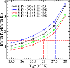
Figure 2: Ionization balance for He i-ii and Si iii-iv. The ratio of equivalent widths (EWs) for selected pairs of He and Si lines are shown for models with $\log g$=3.0 and T_eff =2.55-2.8$\times$10⁴ K. Each square represents the model that matches the observed ratio of the equivalent widths (EWs) of the lines. The horizontal dashed lines show the equivalent width ratios measured from optical data, while the vertical dashed lines show the projection of the matching model EW to the temperature axis. We estimated the measured EW ratio errors. The maximum is around 1 %, which would influence our lower temperature limit by $\lesssim$100 K.

Figure 2 shows the analysis for the ionization balance of He i-ii and Si iii-iv. The ionization balance of He i-ii yields an effective temperature approximately $2.65\times 10^{4}$ to $2.68\times 10^{4}$ K while the Si iii-iv ionization balance yields a value $\sim$ $2.68\times 10^{4}$  to $2.75\times 10^{4}$ K. From these results we concluded that the effective temperature of $\epsilon$ Ori is T_eff=27000$\pm$500 K. In the UV, Si iii $\lambda$1312 shows a strong dependence on temperature. This line yields a slightly lower temperature of T_eff=26200 K. Nevertheless, Fe iv-v lines and the O iv $\lambda\lambda$1342,1343 lines support a value of 27000 K. The Si iii-iv $\lambda\lambda$1417,1416 lines provide a temperature estimate of 27500 K.

Table 5: Wind parameters of $\epsilon$ Ori from optical and UV data. The mass-loss rate for both HIPPARCOS distances is given.

Model	$f_{\infty}$	$\dot{\rm M}$/$\sqrt{f_{\infty}}$a	$\dot{\rm M}$/$\sqrt{f_{\infty}}$b	$v_{\infty}$	$\beta$	$\xi_{max}$	$v_{cl}$
		M⊙ yr-1	M⊙ yr-1	km s-1		km s-1	km s-1
A	0.1	1.55$\times$10-6	2.70$\times$10-6	1800	2.0	200	40
B	0.05	1.66$\times$10-6	2.80$\times$10-6	1800	2.0	200	30
C	0.01	1.75$\times$10-6	2.90$\times$10-6	1800	2.0	200	20
D	1.0	1.40$\times$10-6	2.55$\times$10-6	1800	2.0	200	–

• HIPPARCOS catalog (Perryman et al., 1997) ($d$=412 pc)

• HIPPARCOS catalog (van Leeuwen, 2007) ($d$=606 pc)

Photospheric microturbulence velocity ($\xi_{min}$) was estimated to be between 15 and 20  km s^-1 using He i lines. The silicon triplet (4554-4576 Å) suggests a $\xi_{min}$ close to the lower limit, 15  km s^-1 while the UV Si iii multiplet indicates a microturbulence closer to 10  km s^-1(Fig. 3). The variations do not change the reported limits for temperature and gravity.

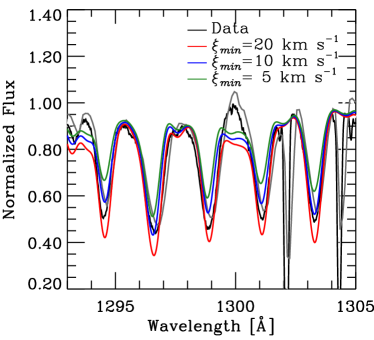
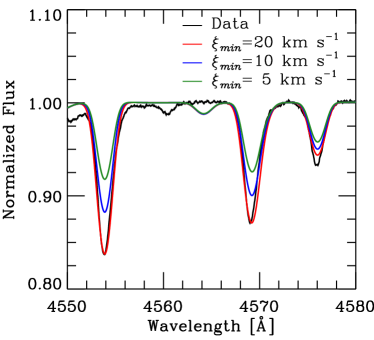
Figure 3: Dependence of UV and optical Si iii lines on photospheric microturbulence ($\xi_{min}$). In the left panel, the black line represents the GHRS data and the gray line COPERNICUS data. Profiles for three photospheric microturbulent velocities are shown: 20  km s^-1 (red), 10  km s^-1 (blue) and 5  km s^-1 (green).

Figure 3 shows the line profiles for optical and UV Si iii lines. The models correspond to three values of turbulence velocity: 20  km s^-1 (red), 10  km s^-1 (blue) and 5  km s^-1 (green). We found divergence between the UV and optical silicon lines – the UV (Si iii $\lambda\lambda$1290-1310) complex suggests $\xi_{min}\sim$10  km s^-1  while the optical triplet Si iii $\lambda\lambda$4550-4580 requires a value of $\xi_{min}\sim$20  km s^-1. Furthermore, the Fe iv $\lambda\lambda$1450-1500 and Fe iv $\lambda\lambda$1600 -1700 lines rule out $\xi_{min}$ lower than $\sim$10  km s^-1.

The discrepancy between UV and optical Si iii lines can be overcome by increasing the silicon abundance by a factor of $\sim$1.2 with $\xi_{min}$=15  km s^-1. However, such a value is incompatible with other optical lines (e.g. N iii $\lambda$4098 and C iii $\lambda\lambda$4648-4654).

The rotation and macroturbulence velocities were estimated simultaneously from fitting the line shapes. We estimated values of 40-70  km s^-1 for rotation and 70-100  km s^-1 for $v_{macro}$. That rotation value is lower than previously reported ($v\sin i=91$  km s^-1 by Howarth et al. (1997)). However upon close examination we found this rotation rate accurately fits some optical line profiles, such as those belonging to Si iii $\lambda$4554-4576. Rotation is analyzed in § 5.7.

5.2 Wind Parameters

We calculated models for four different values of filling factor ($f_{\infty}$). The best fitting parameters for each of these models are shown in the Table 5. We use capital letters as reference for the subsequent analysis. The best synthetic spectra for each filling factor from UV to optical together with data are shown in Appendix A.

5.2.1 Mass-loss rate

Because of the strong sensitivity of the H${\alpha}$ line profile to the mass-loss rate, it is possible to attain high precision for this parameter through fitting its line strength. We found $\dot{\rm M}$/$\sqrt{f_{\infty}}{\approx}$1.6$\times$10^-6  M_⊙ yr^-1 for $\epsilon$ Ori ($d$=412 pc). The mass-loss rate for each filling factor is shown in Table 5. As expected, Ṁ$/\sqrt{f_{\infty}}$ is almost independent of $f_{\infty}$, and is lower than the value $\dot{\rm M}$$\sim$2$\times$10^-6  M_⊙ yr^-1estimated by Searle et al. (2008) and Crowther et al. (2006). The main reason for the discrepancy is their adopted lower values for $\beta$ (1.1 and 1.5, respectively). A lower $\beta$ value yields lower densities in the H$\alpha$ formation region, and hence a higher mass-loss rate is required to fit the line emission. As these values were computed using mainly H$\alpha$, its variability will increase the uncertainty of the mass-loss rate. Morel et al. (2004) and Thompson & Morrison (2013) reported H$\alpha$ variability in its shape profile and strength. The results shown here are based on data collected on a specific date, and don’t show H$\alpha$ variability during observations. We changed the mass-loss rate in order to obtain the strongest and the weakest line from Thompson & Morrison’s profile. The corresponding values are 4.8$\times$10^-7 and 2.8$\times$10^-7  M_⊙ yr^-1 respectively (assuming $\beta=2$, $f_{\infty}=0.05$ and $d=412$ pc). The variation is approximately 30% about our derived mass-loss rate of 3.6$\times$10^-7  M_⊙ yr^-1. This shows that small changes on Ṁ yield larges changes in the H$\alpha$ profile. A full variability analysis is necessary to improve our conclusions about $\dot{\rm M}$ for $\epsilon$ Ori, but this kind of analysis is beyond the scope of this paper.

In our analysis we did not include the infrared (IR) and radio spectral regions, but we can compare our results with those from previous studies. Blomme et al. (2002) used radio fluxes from 3.6 and 6.0 cm and computed a $\dot{\rm M}$$\sim$1.66$\times$10^-6  M_⊙ yr^-1 assuming a smooth model. This is consistent with our estimate, but only if clumping persists into the radio region (our model fluxes at 6.0 cm is $\sim$0.7 mJy, while the mean of reported Blomme et al.’s ones is $\sim$0.74$\pm$0.13. mJy.). Models by Runacres & Owocki (2002) indicate that structure can persist into the radio region and may influence radio diagnostics. On the other hand Puls et al. (2006) found a difference between stars with strong and weak winds. For strong winds their analysis suggested that wind clumping declined into the radio region while for weak winds they found similar clumping in the inner and outer wind. In future work radio and millimeter fluxes should be incorporated into the analysis.

Using IR observations Repolust et al. (2005) obtained $\dot{\rm M}$$/\sqrt{f_{\infty}}$=3.7$\times$10^-6  M_⊙ yr^-1 while Najarro et al. (2011) derived $\dot{\rm M}$$/\sqrt{f_{\infty}}$=2.0$\times$10^-6  M_⊙ yr^-1 (for the comparisons we scaled the reported values to our distance and $v_{\infty}$). The $\dot{\rm M}$ derived by Najarro et al. is consistent with our estimate while that of Repolust et al. is a factor of $\sim$ 2 higher.

UV lines are less sensitive than H$\alpha$ to changes in $\dot{\rm M}$/$\sqrt{f_{\infty}}$. Therefore, we use UV lines only to confirm our H$\alpha$ values. Moreover, UV line strengths also depend on ionization structure and some of them also on the X-ray emission (e.g. N v and C iv). The X-ray independent and non-saturated UV line C iii $\lambda$1176 confirmed the Ṁ(H$\alpha$) values. Si iv $\lambda\lambda$1394-1402 was not well reproduced, likely because of vorosity-porosity effects, so it was disregarded in the analysis (§ 6).

5.2.2 Velocity profile

The wind acceleration parameter ($\beta$) strongly affects the H$\alpha$ profile (Hillier, 2003). The H$\alpha$ profiles calculated for $\beta$=1.0, 1.5 2.0 and 2.2 are shown in Figure 4. From this figure, we concluded that the better $\beta$ value is around 2.0 (values lower that 1.8 or higher that 2.2 were unable to reproduce the profile). This value is higher than others previously calculated for early B-supergiants (e.g. Kudritzki et al., 1999; Crowther et al., 2006; Searle et al., 2008). For each $\beta$ we explored a wide range for $\dot{\rm M}$/$\sqrt{f_{\infty}}$, however we were unable to match the observed line profile for low $\beta$ values.

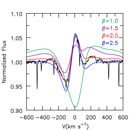
Figure 4: H$\alpha$ profiles for different $\beta$ values: 1.0 (green), 1.5 (purple), 2.0 (red) and 2.5 (blue). Black line represents the optical data. Each line profile was computed with the $\dot{\rm M}$ that matches the observed line strength.

Crowther et al. ($\beta$=1.5) used two sets of optical data for $\epsilon$ Ori, but the line shape was not reproduced in either case. They obtained high velocity wing emission that is not detected, and they were unable to reproduce the blue absorption observed in H$\alpha$ profile.

Searle et al. ($\beta$=1.1) do not show their H$\alpha$ profile; we tried to fit this line with their $\beta$ value by tuning other wind parameters but we were unable to reproduce the line shape with such a low $\beta$ value.

In the above works other Galactic early-type B-supergiant stars were also analyzed. The derived $\beta$ values are between 1.0 and 1.5. For Small Magellanic Cloud (SMC) B0-B1 supergiants, Trundle et al. (2004) also found $\beta$ values lower than ours. Evans et al. (2004) analyzed two B0Ia stars within a sample of supergiants from the Magellanic Clouds: AV235 and HDE 269050. They found $\beta$ parameters of 2.50 and 2.75, respectively.

Spectral variability of H$\alpha$ could be one reason for the discrepancy between our values and those derived from previous works. Thompson & Morrison (2013) reported profile variability on a time scale of weeks. This variability is still not understood (see also Martins et al., 2015). An alternative to be investigated in the future is a different radial dependence for the filling factor. Runacres & Owocki (2002) predicted that the clumping factor ($f_{cl}=1/f$) grows until 10-50 R_∗ and then falls in the outer wind regions. However, Puls et al. (2006) shows that for denser winds high clumping factors are present close to the stellar surface. $\epsilon$ Ori doesn’t show a high mass-loss rate, but a different clumping distribution should be investigated in combination with other $\beta$ values.

The $v_{\infty}$ and $\xi_{max}$ parameters were estimated together using the blue absorption wing of UV lines, especially C iv $\lambda$1550 and C iii $\lambda$1175. We found that the value of $v_{\infty}$ lies between 1700 and 1800  km s^-1, while the wind turbulence velocity is $\xi_{max}{\sim}$200  km s^-1.

The values calculated here are between the previous ones calculated by Crowther et al. (2006) and Searle et al. (2008) (1600 and 1910  km s^-1 respectively). The C iii $\lambda$1175 profile rules out a value of 1600  km s^-1 for $v_{\infty}$, since a value of $\xi_{max}\gtrsim$300  km s^-1 is necessary in order to fit the blue absorption wing. Such a high value for $\xi_{max}$ distorts the Si iv $\lambda$1400 profile and the C iv $\lambda$1550 blue absorption wing.

5.2.3 Clumping

Besides the mass-loss rate, we also changed $v_{cl}$ (the point where the clumping starts) aiming to optimize the H$\alpha$ profile. The best values for $v_{cl}$ for each $f_{\infty}$ are shown in Table 5 and are between 20 and 40  km s^-1. Figure 5 shows the effect of $f_{\infty}$ on different lines in the optical and UV. We found that S iv $\lambda\lambda$1062,1073 and N iv $\lambda$1718 yield a low value for $f_{\infty}$ ($\leq$0.01). The same was found for P v $\lambda\lambda$1118-28 (not shown in the figure). On the other hand, the optical lines yield a moderate value between 0.05 and 0.1. These discrepancies cannot be corrected by altering the mass-loss rates without spoiling the H$\alpha$ profile. It is possible to alter the abundances until the model fits the lines, but the derived values for a reasonable value for $f_{\infty}$ are too low to be plausible, especially for sulfur.

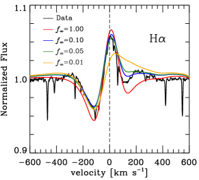
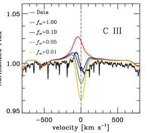
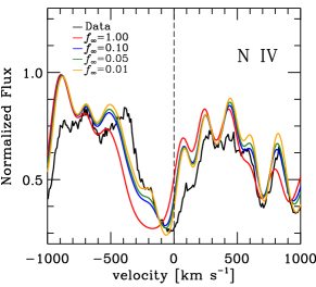
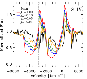
Figure 5: Shown is the effect of clumping on selected optical and UV lines. Upper panels correspond to the optical lines H$\alpha$ and C iii $\lambda$5697, while the lower ones correspond to UV lines S iv $\lambda\lambda$1062,1073 and N iv $\lambda$1718.

5.3 Abundances from UV and Optical

We chose model “A” to estimate the abundances of CNO, Si and Fe. The lines selected for estimating the abundances are not affected by wind emission, hence it is irrelevant which model, from Table 5, we choose. Solar abundances for Si and Fe fit the optical and UV spectra to within 10%. Because of this, we fixed their abundances to solar values and concentrated our analysis on CNO abundances. Nevertheless, as it was noted above, a silicon abundance of 1.2 Si_⊙ helps to reconcile the fit to the UV and optical Si iii multiplets.

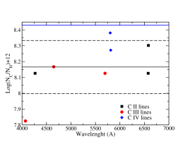
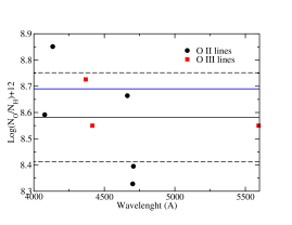
Figure 6: Abundances for CNO. The dots show the abundance that fits each line for each ion and species. The black line is the mean of those abundances, the dashed lines are the mean $\pm$ the standard deviation and the filled blue line represents the solar value.

Figure 6 shows three panels. In each of these panels the y-axis shows the abundance estimate obtained from each transition and the x-axis shows the line wavelength. The numerical abundances are relative to hydrogen, expressed as: $\log(N_{X}/N_{H})+12$. The filled black line represents the mean value (simple average) while the dashed lines represent the standard deviation of those measurements.

Table 6 shows the mean CNO abundances and their standard deviations, the N/C and N/O abundance ratios, and the corresponding solar values. These ratios are calculated as: $[$N/(C,O)$]$= $\log(N_{N}/N_{(C,O)})_{*}-\log(N_{N}/N_{(C,O)})_{\odot}$. The other three columns show previous abundance estimates from Crowther et al. (C06) and Searle et al. (S08).

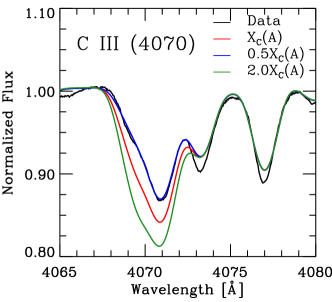
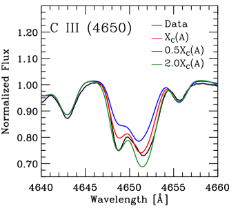
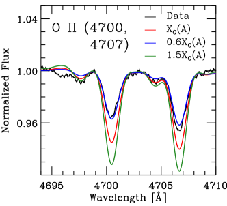
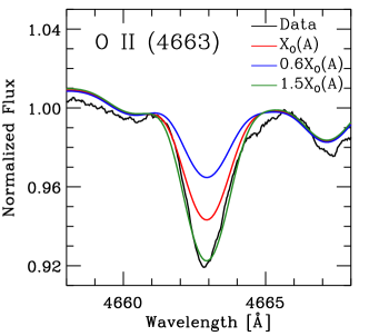
Figure 7: Abundance discrepancy from lines of the same ion: C iii (upper panels) and O ii (lower panels). C iii $\lambda$4070 requires half the abundance needed by C iii $\lambda$4650 while the O ii $\lambda$4663 abundance is 2.5 times larger than that found from O ii $\lambda\lambda$4700,4707.

Our values for $[$N/(C,O)$]$ show a small nitrogen enhancement and carbon and oxygen depletion. This provides evidence for CNO processed material at the star surface. Nevertheless, when compared with C06 and S08, our values are closer to the solar ones.

Table 6: CNO abundances from optical and UV data. $[$N/C,O$]$=$\log(N_{N}/N_{C,O})_{*}-\log(N_{N}/N_{C,O})_{\odot}$

Species	This Work	$\sigma$(dex)	S08	C06	Solar
C	8.16	0.16	7.66	7.95	8.43
N	7.90	0.18	7.31	8.15	7.83
O	8.58	0.17	8.68	8.55	8.69
Si	7.51	0.04	7.51	7.51	7.51
Fe	7.50	0.04	7.50	7.50	7.50
$[$N/C$]$	+0.33	–	+0.26	+0.8	0.00
$[$N/O$]$	+0.15	–	-0.49	+0.5	0.00

The abundance determinations typically scatter within a factor of 2 either side of the mean, as shown in Figure 6. Figure 7 shows the sensitivity of several lines to the abundance. For instance, C iii $\lambda$4070 requires half of the abundance predicted by C iii $\lambda$4650. Similarly the O ii $\lambda\lambda$4663 abundance is 2.5 times larger than that obtained with O ii $\lambda\lambda$4700,4707.

The possible causes of the abundance discrepancies are many — complex NLTE effects, deficiencies in the atomic models, blending, issues related to microturbulence and macroturbulence. For example, it was pointed out by Nieva & Przybilla (2006) that NLTE effects can cause discrepancy between the abundances estimated using C ii lines 4267 Å and 6587-82 Å. We didn’t find strong discrepancies among these lines — the difference is not larger than 0.2 dex. Likewise, complex NLTE effects could affect the abundance estimates of other lines such as C iii (Martins & Hillier, 2012) and N ii-iv (Rivero González et al., 2011, 2012b, 2012a).

5.4 Wind Parameters from X-rays

We performed the fit procedure as described in Section 4.1.2, using the Chandra and XMM-Newton data simultaneously. The results for each of the models described above (A, B, C and D) are shown in Table 7. For each model we found that low temperature ($\sim$1-3$\times$10⁶ K) plasmas are necessary to account for the N vii Ly$\alpha$, N vi He$\alpha$ and C vi Ly$\alpha$ lines, as well as the He-like line of Ne ix He$\alpha$. Similarily, a hot component is needed to account for Si xiii, Mg xii and Mg xi lines. The Si xiv Ly$\alpha$ at 6.18 Å is not detected by Chandra, and hence the hottest plasma temperature is less than 1$\times$10⁷ K. These temperatures are consistent with the distribution of heating-rates computed by Cohen et al. (2014b) for $\epsilon$ Ori. They show that $\epsilon$ Ori has low heating rates for T$\gtrsim$10⁷ K.

Figures 8 and 9 show the Chandra and XMM-Newton data with the models A (green), B (blue), C (orange) and D(red), respectively. The fits are reasonable for most lines, except for Ne x $\lambda$12.13 which is too weak in all our models. The fit of this line is strongly coupled to the fitting of the Mg xi-xii lines — better Ne x line profiles were obtained when those lines were excluded from the fits but the model Mg lines are too strong. The whole fit improves if we lower the Mg abundance approximately 10%. On the other hand, Drake & Testa (2005) and Cunha et al. (2006) have suggested that the currently accepted solar abundance of neon might be underestimated. We computed models increasing the Ne abundance by 40%, although the Ne x $\lambda$12.13 profiles improve, the emission in the Ne He-like triplet is overestimated.

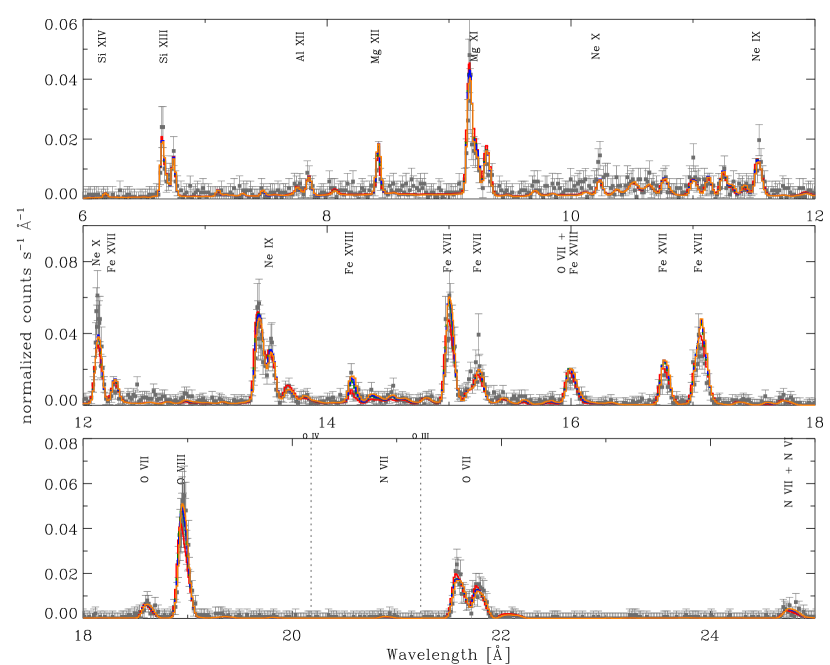
Figure 8: Chandra data (gray squares with error bars) and best X-ray models for A(green), B(blue), C(orange), and D(red). Dots lines show the K-shell ionization threshold for O iii and O iv. The models are indistinguishable except for a few lines.

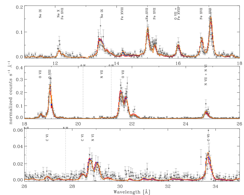
Figure 9: XMM-Newton data (gray squares with errors bars) and best X-ray models for A(green), B(blue), C(orange), and D(red). Dots lines show the K-shell ionization threshold for O iii, O iv, N iii and N iv.

Table 7 shows the spatial distribution of the emitting plasmas. Typically the coolest plasma is found to exist at larger radii than the hottest plasma. Specifically, for 10⁶ K plasma R₀ is around 4-4.9 R_∗, for the 2-3$\times$10⁶ K plasma R₀ is between $\sim$3-4.7 R_∗, and for the 7$\times$10⁶ K plasma R${}_{0}\sim$2.1-2.9 R_∗. We note that the onset radii are above the height where clumping starts ($v_{cl}$=20-40 km s^-1=$v(r{\sim}$1.12-1.23 R_∗)). The same result was found by Cohen et al. (2011) in their analysis of HD 93129A – the estimated onset radii were larger than R_cl.

Table 7: Plasma parameters for the best models that fit Chandra and XMM-Newton data simultaneously.

TX	R0	$f_{X}$		TX	R0	$f_{X}$
106 K	R∗	10-3		106 K	R∗	10-3
model A				model B
1.0	4.84	26.93		1.0	4.45	50.67
2.0	4.56	7.22		2.0	4.73	14.70
3.0	3.05	4.76		3.0	2.95	8.31
7.0	2.60	0.34		7.0	2.63	0.72
model C				model D
1.0	3.89	123.0		1.0	6.10	12.79
2.0	4.72	62.03		2.0	3.40	1.111
3.0	2.77	24.58		3.0	3.85	1.66
7.0	2.89	4.26		7.0	2.14	0.029

The present analysis allows for contributions from different plasmas (T_X and R₀) to each X-ray line. Here, the principal lines in the Chandra and XMM wavelength range are fitted consistently with the same model. Thus, we found that short wavelength lines have flux contributions from hot plasmas, unlike long wavelength lines that mainly have contributions from colder plasmas. The same trend was found by Hervé et al. (2013) (their Fig. 4) in their analysis of the RGS spectrum of $\zeta$ Pup.

The findings indicate that the shortest wavelength lines start to be emitted from regions close to the stellar surface in the wind, while the longer wavelength lines originate from the outer regions. This result is confirmed by line width measurements – lines with a higher wavelength have larger line widths (Tables 8 and 9).

Waldron & Cassinelli (2007) argued that this trend, found in some supergiants, doesn’t indicate that the cooler shocked plasma is formed only in the outer wind regions. Rather, the inner cool gas is not seen due to optical depth effects. In other words, the wavelength dependence of continuum X-ray optical depth means that long-wavelength photons produced close to the surface are absorbed by the optically thick wind. Cohen et al. (2014a) emphasized optical depth effects as an explanation. They didn’t find a significant trend in their sample of O stars ($\epsilon$ Ori included). However data for some stars is suggestive of longer wavelength lines from lower-temperature plasma being formed farther out in the wind. Figure 10 illustrates this point. It shows curves of the radius where the continuum X-ray optical depth equals unity, $r(\tau_{x}=1)$, and the wavelengths of the main H-like and He-like lines. Utilizing Figure 10 in conjunction with Table 7 it is apparent that every “observed” plasma exists above the $r(\tau_{x}{=}1)$ where the transmission factor is high for each wavelength, as was pointed out by Leutenegger et al. (2010). Despite the high R₀, we estimate that $\sim 70$% of the emitted X-rays are absorbed by the wind – the X-ray absorption is very signifcant for $\lambda\gtrsim$12 Å.

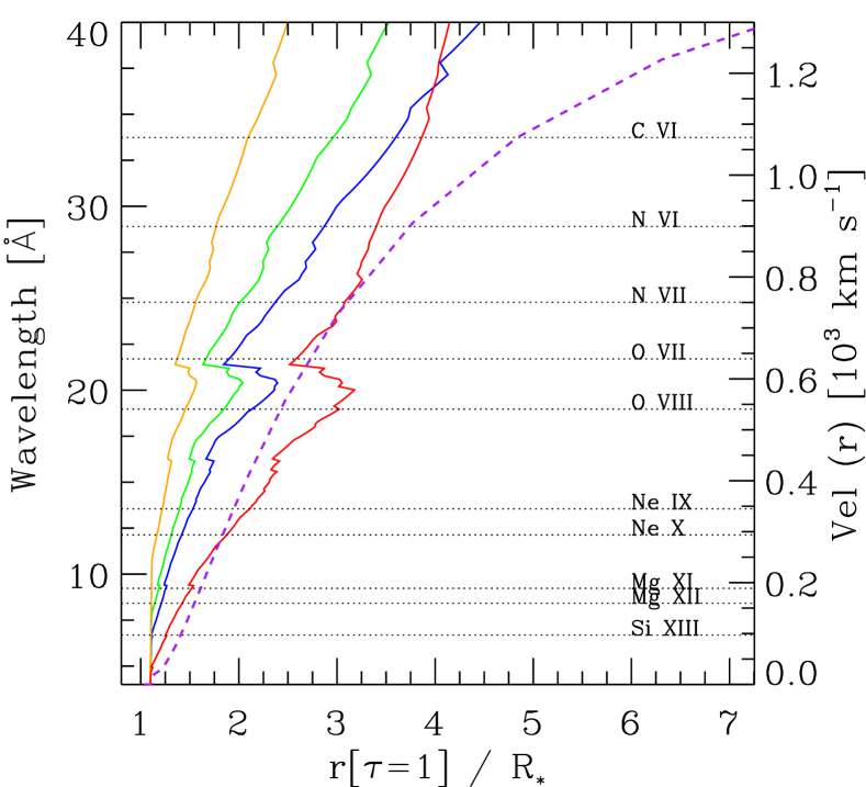
Figure 10: The radius where the continuum optical depth is equal to 1 ($R_{\tau_{X}=1}$) for wavelengths from 4 to 40 Å. The curves are as follows: model A (blue), B (green), C (orange) and D(red). The dashed purple line shows the velocity profile through the wind while the black dashed lines show the wavelengths for the main H-like and He-like lines. As we lower $\dot{\rm M}$ the radius at which $\tau_{X}=1$ is also reduced. The less steep increase of $R_{\tau_{X}=1}$ for the smooth model at longer wavelengths ($\lambda>30\,\AA)$ is caused by ionization of He⁺ to He⁺⁺. See Section 6.

Figures 11 and 12 show the calculated line profiles for some H-like and He-like X-ray lines together with data from Chandra and XMM. H-like profiles are centered at the red component of the doublet, whilst He-like profiles are centered at the red component of the intercombination doublet. A visual inspection shows that the observed lines are slightly blue-shifted, and that every model reasonably reproduces the profiles, with the exception of model “D” (red line). This is especially clear when we look at the O viii profile.

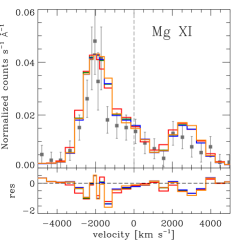
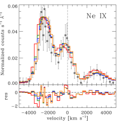
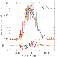
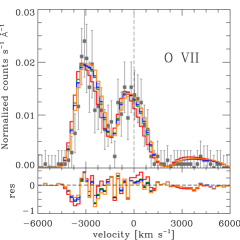
Figure 11: Observed Chandra (squares) and synthetic line profiles corresponding to model A (blue), B (green), C (orange) and D (red). Note the primary difference among the models is the notable line asymmetry for the highest $\dot{\rm M}$ model, especially for the longer wavelength lines where wind opacity is higher. Lower panels show the residuals.

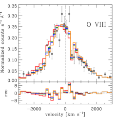
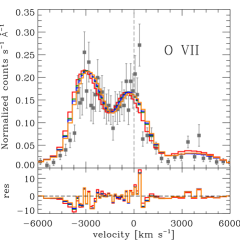
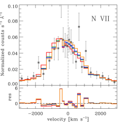
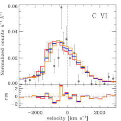
Figure 12: Observed XMM-Newton (squares) and synthetic line profiles corresponding to model A (blue), B (green), C (orange) and D (red). Lower panels show the residuals.

Table 8: Statistics “C” from fits of H-like (Ly$\alpha$) and He-like Chandra lines. The values in the parentheses are the number of bins used for each line fit.

Ion	Si xiii	Mg xii	Mg xi	Ne x	Ne ix	O viii	O vii	N vii
	(35)	(22)	(50)	(30)	(80)	(50)	(145)	(66)
$\sigma$a	–	350	–	610	–	706	–	765
C(A)	31.39	17.25	55.93	23.91	67.19	54.36	132.66	79.42
C(B)	31.66	17.81	56.62	24.66	68.22	50.69	131.47	79.22
C(C)	34.75	18.63	58.89	27.15	70.07	48.82	133.50	80.20
C(D)	28.27	15.91	54.76	31.93	78.95	88.40	153.49	78.92

• The HWHM for each line in  km s^-1 of the Gaussian fit to the line profile.

Table 9: Statistics “C” from fits of H-like (Ly$\alpha$) and He-like XMM lines

Ion	Ne x	Ne ix	O viii	O vii	N vii	N vi	C vi
	(20)	(68)	(38)	(88)	(46)	(106)	(45)
$\sigma$ a	610	–	706	–	765	–	880
C(A)	18.46	64.61	58.56	109.60	56.51	164.83	69.97
C(B)	18.32	64.11	57.28	107.53	56.52	166.93	69.81
C(C)	18.37	64.10	57.79	104.16	57.47	165.10	71.16
C(D)	19.64	68.66	73.24	126.13	56.61	159.85	71.82

• The HWHM for each line in  km s^-1

In order to clarify which models match the observations we calculated the “C” statistics for each H-line and He-like line model profile. To do this we allow the flux for each model profile to be a free-parameter, and choose the scaling that minimizes the C statistic. The results are shown in Tables 8 and 9 for Chandra and XMM data respectively. From the values, we confirm that the smooth wind model (model “D”) can be ruled out based on the fit to O viii and O vii ($\Delta C{\gg}$6.63 when compared to the minimum among the other values of the same line), although the Ne ix, N vii and C vi lines also have inferior-C statistics for model D. The other models, and other lines, have similar values for the C statistics, and can be considered statistically indistinguishable

From the results described above we conclude that the mass-loss rate required to fit the X-ray spectrum of $\epsilon$ Ori is $\lesssim$ 4.5$\times$10^-7  M_⊙ yr^-1, which confirms the UV and optical results that the $\epsilon$ Ori wind is clumped. Furthermore, these values of mass-loss rate agree with those reported by Cohen et al. (2014a) for the same star using exclusively Chandra data. Cohen et al. (2014a) computed two values for the mass-loss rate of $\epsilon$ Ori: 6.5$\times$10^-7  M_⊙ yr^-1 and 2.1$\times$10^-7  M_⊙ yr^-1. The former comes from excluding from their analysis the lines (3 lines from 10) which possibly are affected by resonance scattering (Leutenegger et al., 2007), while the lower value results from including all of the lines of their spectrum. As pointed out above R₀ values move the X-ray line formation region out of the absorbed part of the inner wind, making it unnecessary to include the resonance scattering to make more symmetric lines. Including resonance scattering effects in the analysis could have an influence on the computed $\beta$ and R₀ values, but not in strong way due to the low density of $\epsilon$ Ori’s wind (which is less than that of $\zeta$ Pup).

Models using a different wind acceleration parameter ($\beta=1.0,1.2$) were also calculated. Wind and photospheric parameters from model “A” were adopted. For short wavelengths ($\lambda{\lesssim}$14 Å) the model yields profiles that cannot be distinguished from the $\beta$=2 model. But for longward wavelengths a better fit is provided by the $\beta$=2 model. Specifically, the models fail to reproduce the He-like O vii line, and the Ly$\alpha$ lines of N vii and O viii. For this set of lines the model profiles are too asymmetric when compared with the data. Quantitatively, the “$C$” values increase $\sim$20-100% for models with $\beta$=1-1.2 when compared with $\beta$=2 profiles (e.g. $\Delta C{\sim}45$ in the case of Ly$\alpha$ O viii). In the case of He-like N vi and Ly$\alpha$ C vi lines the increase in “$C$” is approximately 5-10% ($\Delta C{\sim}3.0{-}6.0$).

The plasma temperatures were fitted again as described in Section 4.1.2. The lower temperatures are the same as those calculated above, but a better fit was achieved by switching the hottest plasma to 8$\times$10⁶ K. The onset radii are closer than those from the model with $\beta$=2 because models with lower $\beta$ yield higher velocities in the region from R=1.1-6.1 R_∗. The coolest plasma (10⁶ K) has $R_{0}=2.16R_{*}$, the plasma of 2$\times$10⁶ K has $R_{0}=6.1R_{*}$, while the plasmas of 3$\times$10⁶ K and 8$\times$10⁷ K have $R_{0}$ values of 1.9 R_∗ and 1.4 R_∗ respectively.

5.5 Abundances from X-rays

The metal abundances, relative to hydrogen, could be estimated using the continuum emission relative to line emission. But in the case of XMM data, most of the spectral range is contaminated by line emission. However, a narrow region around the nitrogen lines shows weak or no lines. The modeled continuum in this region is almost 50% below that observed. To fit the continuum it would be necessary to both scale the model emission measures and to lower the metal abundances by approximately $\sim$50% in oder to preserve the fit to the lines. By limiting the fit to nitrogen lines region a good match for both the continuum and those lines can be found. However, most of continuum comes from the hottest plasma (T${}_{X}{=}$7$\times$10⁶ K) which spoils the fit to the shortward wavelength spectrum. Furthermore, as it’s shown in the figures 8 and 9 the shortward continuum is fitted fine by our models. This discrepancy could be due to a lack of pseudo-continuum weak lines in apec as suggested by Zsargó et al. (in preparation).

From the reasons exposed above, it was not possible to derive metal abundances relative to hydrogen – only the relative abundances among metals. We searched for some trends by measuring the fluxes for the main X-ray metal lines from the data, and compared them to the corresponding model fluxes.

The observed fluxes were calculated by fitting Gaussian profiles for each H-like line and He-like triplet. Also, we calculated the fluxes for Fe lines around 15 Å and 17 Å. Each of these blends (two lines around 15 Å and two more around 17 Å) were treated separately, but their fluxes were added in order to compare them with the model values whose fluxes were estimated taking into account the whole blend.

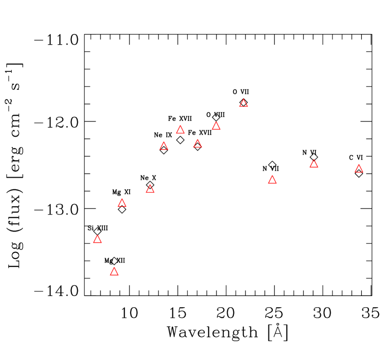
Figure 13: X-ray line fluxes. The observed fluxes are shown as black diamonds while the values for model “A” are red triangles.

Figure 13 shows the measured X-ray line fluxes and the ones from model “A”. There are not strong trends that would suggest changes in abundances. The model line fluxes for N vii Ly$\alpha$ and N vi are too small compared with observations – increasing the nitrogen abundance by 30% would bring them into better agreement.

In order to quantify the consistency of the abundances we calculated lines flux ratios that show a low temperature dependence. We used the ratios expressed in Equations 4 and 5. The dependence of these flux ratios on temperature is shown in Figures 14a and 14b for a grid of models with the same abundances as in model “A” (solid lines) and in a model with solar abundances from Asplund et al. (2009)(dashed lines). For each set of abundances we also examined the effect of the starting X-ray emission radius (i.e., R₀). The line ratios depend on R₀ due to the strong dependence of the opacity on wavelength. As longer wavelength lines are less attenuated at higher R₀, the N(H$\alpha$)/O(H$\alpha$+He) ratio will increase with R₀. Also, higher temperatures favour the presence of N vii, while O viii + O vii is almost constant. This highlights the need for a reliable emission model if abundances are to be derived from X-ray data.

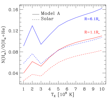
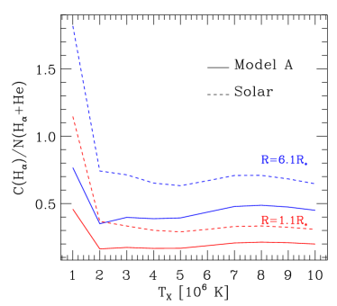
Figure 14: Temperature behavior of line ratios calculated with Equations 4 and 5 with the temperature of emitting plasma (T_X). Blue lines correspond to models in which the X-ray emitting plasma starts at R₀=6.1R_∗ while the red lines correspond to models with R₀=1.6R_∗.

Table 10 shows the values of these ratios for model “A”, the same model but with an nitrogen abundance enhanced by a factor of 1.3 compared with observation (with errors in parentheses). The enhanced nitrogen model improves the agreement between the observed and model values. Such a small correction is within the error estimated for the N abundance determined from optical and UV data. We conclude that the relative abundance values derived from the X-ray analyses are statistically consistent with those derived from UV and optical analyses, and indicate a modest enhancement of N relative to both C and O.

Table 10: CNO abundances from X-ray data. Errors on measured values are in parentheses.

	Measured	Model A	Model A 1.3 N	Solar
R(N/O)	0.125 (0.008)	0.10	0.12	0.06
R(C/N)	0.357 (0.020)	0.52	0.39	0.98

5.6 Interclump Medium

Zsargó et al. (2008) pointed out that it is necessary to include the interclump medium radiation in order to reproduce the line strength for O vi in $\zeta$ Pup. They showed that when the progenitor of the superion (e.g. N iii for N v) is the dominant ion in the wind, the line optical depth does not depend on wind density, and hence the interclump medium, with its larger volume, can contribute significantly to the strength of superion line profiles. We find that this is also the case for $\epsilon$ Ori.

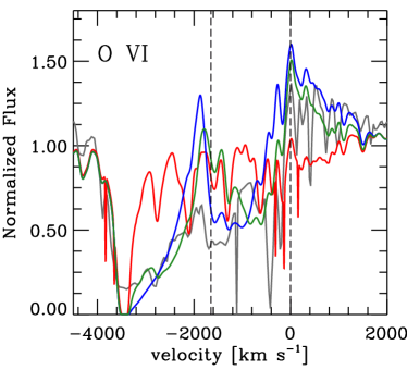
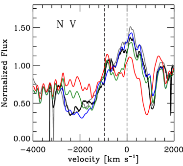
Figure 15: The effect of including the emission of interclump medium. The left panel shows line profiles for O vi $\lambda\lambda$1031,1037 and the right panel line profiles for N v $\lambda\lambda$1238,1242. The black line corresponds to GHRS data, the gray line to COPERNICUS data and the red line to the clumped model “A”. The blue line corresponds to emission from the ICM with a density contrast of 100, and the green line to a density contrast of 200. A much better fit to the profiles is obtained when we allow for the interclump medium.

Figures 15a and 15b show that our clumped model doesn’t reproduce the observed line profiles for N v $\lambda$1238, 1242 and O vi $\lambda\lambda$1031, 1037 (red line) in $\epsilon$ Ori. Using the method of Zsargó et al. (2008), we calculated the emission from a tenuous medium between the clumps. This medium occupies most of the wind volume, with a filling factor $f_{ICM}\sim$0.9-0.95. For this exercise we use the same radiation field from the clumped model – this field is independent of the ICM. We scaled the wind density by two factors, such that $\delta_{ICM}$=$\alpha\times\delta_{cl}$, where the $\delta_{cl}$ is the density in clumps, with $\alpha_{1}$=0.1$\times f_{\infty}$ and $\alpha_{2}$=0.05$\times f_{\infty}$, and assumed that the new component is smooth due to its high filling factor. We calculated this model independently from the clumped model and the hot plasma, but using the same hydrostatic structure.

Figures 15a and 15b show the line profiles calculated for two ICM models corresponding to model “A” with a density contrast between clumped and ICM of 0.1$\times f_{\infty}$=0.01 (blue line) and 0.05$\times f_{\infty}$=0.005 (green line). These values mean that less than 10% of the wind mass is in the interclump medium. The figures show that the ICM models predict line profiles quite similar to those observed for the N v and O vi lines, while the clumped model (red line) fails to reproduce the profiles. We also tried models with even more tenuous interclump media, but the superion line profiles started to weaken.

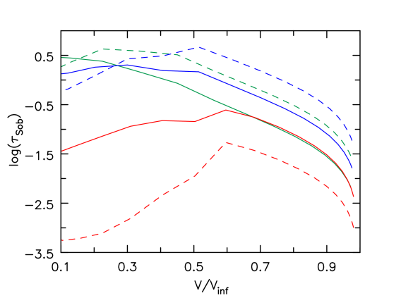
Figure 16: Sobolev line optical depth for N v $\lambda$1238 Å (solid) and O vi $\lambda$1032 Å (dashed). The red lines correspond to the clumped model “A”, while the blue and green lines are for the interclump medium models with density contrasts of 100 and 200 respectively.

Figure 16 shows the Sobolev optical depth of the N v $\lambda$1238 Å and O vi $\lambda$1032 Å transitions for the clumped model (red), and the ICM models with a density contrast of 100 (blue) and 200 (green). It is evident that there is a large increase the in the optical depth in both lines in the ICM models. In their analysis of $\zeta$ Pup, Zsargó et al. (2008) found that the flux of the N v line has contributions from the clumps as well as from the ICM. In the case of $\epsilon$ Ori, we found that most of the line flux comes from the ICM for both the O vi and N v lines. The importance of the ICM medium for these lines arises because of ionization effects.

The ICM has only a very weak influence on other lines, due to its much lower density. The ICM medium is important for the O vi and N v lines because they arise from impurity species whose population is almost independent of density in the wind if they arise from Auger ionization, and if O iv and N iii are the dominant ions. Its influence on $\rho^{2}$ dependent lines, such as H$\alpha$, is insignificant as was already pointed out by Sundqvist et al. (2011), and as confirmed by our own calculations. Sundqvist et al. (2011) notes that macro clumping does lead to a slight weakening of H$\alpha$.

5.7 Rotation

We chose model “A” in order to study in more detail the influence of rotation on the spectrum. We re-calculated the spectrum using the two-dimensional method of Busche & Hillier (2005) as described in Section 4, with the same value for the $v\sin i=70$ km s^-1 estimated from the optical data.

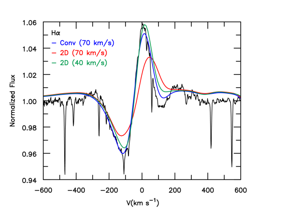
Figure 17: H$\alpha$ profiles from model “A”. Rotation is accounted for using different methods: convolution with a 70  km s^-1 kernel (blue), 2D profile with $v\sin i$=70  km s^-1 (red) and 2D profile with $v\sin i$=40  km s^-1 (green) (see text for details).

Figure 17 shows the H$\alpha$ profile calculated using the convolution method (solid blue line) and the two-dimensional radiative transfer method (solid red line). There is a notable difference between the line profiles. The 2D profile shows weaker absorption and emission, as well as a more extended red wing emission. This strong difference, while at first surprising for such a low rotation rate (70  km s^-1), can be explained from the high value of $\beta$. A high value for this parameter yields a more extended region where the H$\alpha$ line is produced, and where differential rotation can affect the line profile. The main reason for that difference is the dependence of profile shape on the impact parameter as was pointed out by Hillier et al. (2012). This dependence redistributes the fluxes through the line, yielding wider wings emission and lower flux at the line core for both the absorption and emission components. As a consequence, a weaker P Cyg profile is produced.

Table 11: Rotation parameter $v\sin i$, calculated using the fast Fourier transform method for the listed optical lines.

Line	$v\sin i$
Ion $\lambda$ [Å]	km s-1
C ii 4267	46
N ii 3996	33
Si iii 4569	39
Si iii 4576	39
O ii 4592	42
O ii 4597	39
O ii 4663	56
He i 4389	56
He i 4471	55
He i 4715	38
He i 5017	32

In order to reduce the effect described above, we reduced the rotation parameter ($v\sin i$) to 40  km s^-1 and re-calculated the H$\alpha$ profile using the 2D code. The resulting profile is shown in Figure 17 (green line). It is clear that this profile reproduces better the line shape than the former with $v\sin i$=70  km s^-1. The rest of the optical lines, such as Si iii $\lambda\lambda$4453-4576, are well reproduced with 40  km s^-1, but with a macroturbulence of $\sim$90-100  km s^-1 and $\xi_{min}$=15  km s^-1. However, such a low rotation had not been reported until recently – Martins et al. (2015) found the same rotation value for $\epsilon$ Ori in their variability study of OB stars. Their value is based on the fast fourier transform method (see Simón-Díaz & Herrero, 2007; Gray, 2008).

We used the same method to estimate $v\sin i$ based on isolated absorption lines in the optical. The list of lines and the corresponding rotation value are shown in Table 11. All of the $v\sin i$ values are below 70  km s^-1, with an average of 43  km s^-1, almost identical to the value of 40  km s^-1 reported by Martins et al.

6 Discussion

In this paper we have presented the results of a multi-wavelength spectroscopic analysis of $\epsilon$ Ori. We conclude that the main photospheric and wind parameters computed from optical and UV data are completely compatible with those from an X-ray analysis. We concluded that clumped models with $f_{\infty}{<}0.1$ ($f_{\infty}{\sim}0.1$) are able to reproduce the whole spectrum from optical to X-rays. Nevertheless, there are some points that arose from the analysis that need to be discussed more deeply.

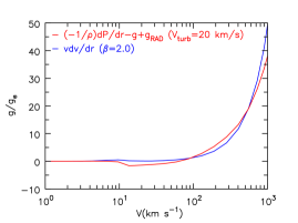
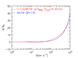
Figure 18: Comparison between velocity profile and acceleration terms from momentum equation (6) divided by the radiative acceleration of free electrons ($g_{e}$). Left panel corresponds to model “A” with acceleration parameter $\beta$=2.0 and $\xi_{min}$=20  km s^-1. Right panel corresponds to the same model, but with acceleration parameter $\beta$=1.5 and $\xi_{min}$=5  km s^-1.

6.1 Hydrodynamical consistency

The high value for $\beta$ derived here presents some problems for consistency with the momentum wind equation. The radiative force is dominated by momentum transfer in optically thick lines. The strength of this force is proportional to a power of the velocity profile slope ($dv/dr$), which is steeper when $\beta$ is low. This means that a high $\beta$ value will yield lower radiative force that may not be able to drive the wind, especially around the sonic point. Further, a larger value of $\beta$ implies that the gravity and the radiative force are almost equal.

The momentum equation for a spherically symmetric wind is:

$$v\frac{dv}{dr}=-\frac{1}{\rho}\frac{P_{g}}{dr}-g+g_{rad},$$ (6)

where $P_{g}$ is the gas pressure, $g=GM_{*}/r^{2}$ and $g_{rad}$ is the total radiative force. Figure 18 shows that the right side (red) and the left side (blue) of Equation (6) for the model “A” (left panel) disagree around the sonic point ($v_{s}{\sim}$17  km s^-1). This also happens for models B and C. It is easy to see that the radiative force is insufficient to match the velocity profile until approximately $\sim$100  km s^-1. The discrepancies between the curves are approximately 40%, but around the sonic point they reach 100%. In the outer wind there are also discrepancies but these can probably be overcome by changes in the velocity law. However, given the assumptions of our modeling (simple radial variation of the filling factor, and the neglect of porosity and vorosity), we do not consider this to be a worthwhile exercise.

Some alternatives have been suggested by Bouret et al. (2012) to overcome this problem. One is to increase the mass-loss rate and the filling factor in order to increase the radiative force and to conserve the spectral fitting. But in the case of $\epsilon$ Ori, as we described above, a filling factor $>$0.1 is incompatible with the X-ray and UV spectra. Even the smooth model doesn’t meet the momentum equations around the sonic point.

As discussed by Bouret et al. (2012) and Lucy (2010), one solution to this problem is to reduce the microturbulent velocity in the vicinity of the sonic point ($\xi_{min}$) and to decrease the $\beta$ value. A lower $\xi_{min}$ will reduce the blocking of continuum radiation coming from the inner atmosphere by the blue line wings, hence boosting the force at the sonic point. A lower $\beta$ will also increase the line radiative force at the sonic point.

The right panel of Figure 18 shows the results for a model with the same parameters of model “A,” but with radiative force calculated for $\beta$=1.5 and $\xi_{min}$=5  km s^-1. The mass-loss rate for this model was adjusted to fit the emission strength of H$\alpha$. The figure shows that even though the curves approach each other around the sonic point the hydrodynamical equation is still not satisifed. Furthermore, lowering the turbulence velocity contradicts the values derived from the spectral analysis.

Another option is to increase the number of levels taken into account in atomic models as well as to include more species in the computation. To investigate this point we calculated a model increasing the number of levels for Fe ions and including Ne, Cl, Ar, and Ca with solar abundances. However, we found that these changes did not improve the momentum balance for the default wind law with $\beta$=2 and a microturbulence of $20\,$ km s^-1.

The discrepancies may be due to some simplifications that are commonly assumed for modeling stellar winds. Microturbulence and macroturbulence are not well understood, as well as their influence on the wind dynamics, especially around the sonic point. Further, variability of line profiles in $\epsilon$ Ori shows that the assumption of a steady-state wind is invalid. Indeed, the difficulty of driving the wind through the sonic point in $\epsilon$ Ori may be explicitly linked with the observed variability of H$\alpha$.

Recent studies of variability in $\epsilon$ Ori have been undertaken by Prinja et al. (2004), Thompson & Morrison (2013) and Martins et al. (2015) based on H$\alpha$, Si iii and He i line profiles. The detected variability has time scales of a few days and those works linked wind variability with photospheric activity that could be caused by stellar pulsations or small scale magnetic fields.

6.2 S iv profiles

As for phosphorus, sulfur has a relatively low abundance, and hence its resonance lines commonly appear unsaturated. As a consequence these lines can provide useful constraints on the mass-loss rate, especially if S³⁺ is the dominant ion in the wind (as it is for $\epsilon$ Ori). The lower left panel of Figure 5 shows the dependence on filling factor of the theoretical profiles for the S iv $\lambda\lambda$1062,1073 doublet. As is readily apparent from the figure, we are unable to reproduce the observed profile shape even with the lowest $f_{\infty}$ value (0.01). The sulfur lines show weak absorption and almost no emission in their P Cygni profiles, in stark contrast to the models that show strong emission and blue absorption. Particularly striking is the absence of absorption at high velocities.

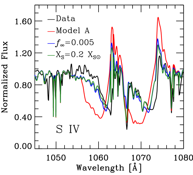
Figure 19: Comparison of the observed line profiles of S iv $\lambda\lambda$1062,1073 with synthetic profiles computed using the model “A” parameters (red), high clumped model (blue) and low sulfur abundance model (green). The black line corresponds to COPERNICUS data.

As shown in Figure 19, we can only “fit” the sulfur doublet if we use an absurdly low abundance ($\sim$0.2 S_⊙ with $f_{\infty}$=0.1) or filling factor ($f_{\infty}{\sim}0.005$). Even with this abundance, the calculated line profiles show more emission than the data. Moreover, an abundance of 0.2 S_⊙ is incompatible with other UV and optical sulfur lines (e.g., S iv $\lambda$1098-1100,4486 and S iii $\lambda$4254). This problem is quite similar to that reported previously with P v $\lambda\lambda$1117,1128 in O stars (e.g. Hillier, 2003; Bouret et al., 2003; Fullerton et al., 2006, 2008; Bouret et al., 2012), and hence we consider similar solutions.

Various solutions have been proposed for solving the P v $\lambda$1117,1128 problem, including the following:

1. Sub-solar abundance. While factors of 2 variation between stars cannot be ruled out, much larger variations are unlikely. In the present case, other S lines rule this out as the main cause.

2. Wrong wind ionization, possibly due to the influence of X-rays. However, the required X-ray flux is higher than observed.

3. Wrong wind ionization, possibly because the bulk of the wind has been shocked and not cooled.

4. The wind is porous spatially, or porous in velocity space (hereafter called vorosity). Porosity will affect both observed X-ray and UV line profiles, whereas vorosity will only affect UV line profiles.

The influence of X-rays on the ionization structure was analyzed by Marcolino et al. (2009) in the context of the weak wind problem of late O dwarf stars. They found that the X-ray luminosity necessary to fit the C iv line strength is approximately 3 dex above the standard value of $L/L_{bol}{\rm{=}-7.0}$. In the same sense, Krtička & Kubát (2009, 2012) explored the influence of X-rays on the phosphorous ion fraction $q(P^{+4})$ aiming to fit the P v lines. They concluded that hard X-ray emission does not have a strong effect on $q(P^{+4})$, whereas XUV (54 - 124 ev) emission yields a $q(P^{+4})$ according to observations. However, X-ray and XUV emission affects the ionization structure of other ions (e.g. C vi, N iv and O iii). This influences the wind terminal velocity value in a non-negligible way, contradicting the observations (Krtička & Kubát, 2012).

In our models the influence of X-rays on the ionization fraction of $S^{+3}$ is less than 5% for the clumped winds ($f_{\infty}=0.01-0.1$), while for the smooth wind the $q(S^{+3})$ is $\sim$25%. Manipulating the $f_{X}$ values for the cold plasma (1$\times$10⁶ K), we computed a model with an enhanced emission in the range of 160-250 Å, just above the ionization threshold of S iv. We found that even though the bluer absorption component of S iv lines is weakened, it wasn’t enough to fit the observed profiles. Furthermore, the XUV radiation needed to fit the lines would be extremely high. Moreover, we obtained reasonable S iv profiles setting R₀ deeper in the wind (R₀=1.1 R_∗). Nevertheless, this change increases the P v abundance in such a way that the lines P v $\lambda\lambda$1118,1128 become too strong. Besides that, such R₀ value is ruled out by X-ray analysis.

Macroclumping (porosity) could reproduce the resonance lines of P v without requiring extremely low mass-loss rates, since optically thick clumps will reduce the effective opacity of the lines (e.g. Owocki, 2008; Oskinova et al., 2007).

Another effect to be taken into account is the so-called “velocity-porosity” or vorosity (Owocki, 2008) that evaluate the effect of a non-monotonic velocity or a velocity field with strong jumps or holes (in the velocity space) on line radiative transfer.

Owocki (2008) showed that vorosity yields a reduction in line absorption but it is low (10-20%). This makes the vorosity effects weak when compared with porosity ones. However, simulation from Sundqvist et al. (2010) and Sundqvist et al. (2011) (see also Sundqvist et al., 2014) point out that vorosity has an important effect on UV profiles that improves the agreement between optical and UV line mass-loss rates.

Using 3D Monte-Carlo simulations Šurlan et al. (2012, 2013) argue that porosity dominates over vorosity effects. An issue with all of these studies is that they primarily utilize the P v profiles – consequently the fit parameters are not unique.

We postulate that the problem of S iv $\lambda\lambda$1063,1073 is analogous to the P v problem, and this gives us a good chance to study clumping in early B stars where P v is not the dominant ion. Furthermore, looking at the COPERNICUS and FUSE catalogs of galactic B stars, it is clear that S iv lines are weak even though we expect that it is the dominant ion in the early B stellar winds.

More evidence for the existence of porosity and vorosity effects can be found in the optical depth ratio of UV resonance doublets. Prinja & Massa (2010) pointed out that this ratio should be equal to the ratio of the oscillator strengths when the clumps are optically thin while for optically thick clumps this ratio is equal to 1. The doublet Si iv $\lambda\lambda$1393,1402 is an excellent candidate for this diagnostic since the oscillator strength ratio is $\sim$2 and the splitting between the components ($\Delta v{\sim}1940$  km s^-1) is large (although it is less than 3600  km s^-1, twice the computed terminal velocity). The data show that the absorption associated with the Si iv doublet components are significantly weaker than the model profiles which are relatively insensitive to the assumed volume filling factor (see second panel from figure A.25). This could be evidence for a reduction in the effective opacity by porosity and/or vorosity.

In the case of S iv $\lambda\lambda$1062,1073, the red component is stronger, with a $gf$ value twice that of the blue component. Thus, if vorosity were the dominant effect models that fit the red component (by adjusting the abundance or filling factor) would underestimate the strength of the blue component. Surprisingly this is not the case – if anything our models do a worse job at matching the bluer component with our model having too much absorption at high velocities. Excluding issues with the observational (and atomic) data, this would suggest that the problem is with the ionization structure of the wind, not an issue with vorosity. Further evidence comes from the shape of the profile. In standard calculations holes in velocity space decrease with velocity, leading to enhanced absorption near the terminal velocity which is not seen in the observed profiles (e.g. Sundqvist et al., 2014). Petrov et al. (2014) suggested that H$\alpha$ could be affected by vorosity, but only for stars below the bi-stability jump. $\epsilon$ Ori is above that limit, furthermore, Sundqvist et al. (2011) showed that this effects are weak on H$\alpha$. Thus H$\alpha$ does not provide a suitable diagnostic of porosity.

6.3 X-rays

An important aspect of our calculations is the derivation of the spatial distribution of the X-ray emitting plasmas in the wind. The R₀ values from Table 7 are higher than previous estimates for other massive stars (see e.g. Leutenegger et al., 2006) or even with those reported by Cohen et al. (2014a) for $\epsilon$ Ori itself. We also found a trend of R₀ vs emitting ion. This trend does not contradict the numerical simulations that predict strong acceleration of some elements of the wind close to the surface (Feldmeier et al., 1997; Runacres & Owocki, 2002; Dessart & Owocki, 2003, 2005), since it could be caused by optical depth effects.

The main reason for the larger R₀ is the high value of $\beta$. With a larger $\beta$ the wind velocity necessary to fit the line widths occurs at larger radii. For a model with $\beta{=}1$, $R_{0}$ is closer to the surface, and variation of R₀ with the temperature is weaker. This is consistent with the finding of constant $R_{0}$ for $\epsilon$ Ori by Cohen et al. (2014a). However, we stress that the link between R₀ and $\beta$ that we found in this work, provides a new challenge for understanding shock formation in the wind and the X-ray emission of massive stars. What does R₀ actually mean and what is behind its relation with wind acceleration? In order to understand the underlying physics of these connections, it is necessary to expand the analysis to more systems.

From the models it is possible to estimate the region where the bulk of each component of He-like lines is emitted. The local contribution to line flux is proportional to $r^{2}n^{2}_{p}(r)\epsilon(r)$, where $\epsilon(r)$ is the line emissivity and $n_{p}$ is the density of the emitting plasma. For instance, for O vii He $\alpha$, the intercombination component ($i$) has its maximum contribution at $\sim$4.6 R_∗. For the forbidden component ($f$), the corresponding value is $\sim$28.5 R_∗. These values show that the different components of He-like triplets are mostly produced in different regions in the wind.

One caveat with our analysis is that our assumption of a small set of single-temperature plasmas to describe the shock emissions is not realistic. In the inner wind the cooling time ($T_{cool}\sim 1/\rho$) for each shock is less than the dynamic time, and hence modeling of the shock structure is required to accurately predict the X-ray emission.This will be explored in the future.

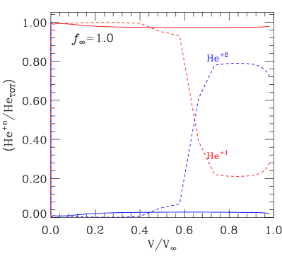
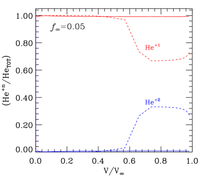
Figure 20: Effect of including X-rays on the ionization structure of He. The solid line corresponds to a model without X-rays, dashed lines correspond to models that include X-ray emission that fit the Chandra and XMM-Newton data.

All of our models yield asymmetric lines, with a lower degree of skewness for models with lower filling factor. The observed blue-shifts of approximately ${\sim}210{\pm}123$  km s^-1 for lines with wavelength $\lambda{\gtrsim}10$ Å provide clear evidence of wind absorption. While a clumped wind is necessary to fit the line profiles we cannot distinguish between the “A” or “B” models with $f_{\infty}$=0.1 and 0.05 respectively. Both models yield adequate X-ray profiles with reasonable mass-loss rates without requiring the inclusion of porosity or resonance scattering effects. This confirms the mass-loss rate derived by Cohen et al. (2014a) that did not use porosity effects to fit X-ray line profiles. Even though, our results and the Cohen et al. ones cannot confirm the absence of porosity. Much higher signal-to-noise X-ray observations are needed if tighter constraints are to be obtained. Moreover, due to the strong variability of H$\alpha$, the influence of non-spherical winds and temporal variability should be considered.

It is generally assumed that X-rays don’t strongly affect the X-ray opacity of the “cool” wind. In the case of $\epsilon$ Ori we found that this is not necessarily true. In $\epsilon$ Ori the X-rays can ionize He⁺ in the outer wind (Fig. 20), reducing the X-ray opacity (see the behaviour at outer regions of the red line in Fig. 10). The effect is largest in the unclumped model. Normally, X-rays don’t strongly affect the dominant ionization stage as X-ray flux is generally small compared with the UV ionizing flux near the relevant thresholds – this is not the case for $\epsilon$ Ori.

The effect of X-rays on He ionization in wind has two consequences: 1) For modeling B or later stars, it is important to take into account the interaction of X-rays with the wind consistently in order to estimate the wind parameters, and not separately as commonly done for O stars. 2) The value of the mass-loss rates computed using X-ray line profiles may be biased toward low values if this effect is not taken into account.

Finally, our preferred models, A and B, show a very strong trend of higher X-ray filling factors for low temperature emission components (see table 7). This model fitting result accounts for both wind absorption and the different emissivities of different plasma temperature components, and thus reflects the instantaneous plasma temperature distribution. These results are broadly consistent with a shock-heating analysis that shows a very strong preference for weaker shocks over strong ones, with almost no shock heating above 10⁷ K.

7 SUMMARY AND CONCLUSIONS

We have presented a multi-wavelength analysis of the early B supergiant $\epsilon$ Ori. This analysis utilizes a modified version of cmfgen  that allows for the radiative interactions between the X-ray emitting plasma and the cool wind.

We get excellent fits to X-ray, UV and optical data. The derived photospheric parameters for $\epsilon$ Ori are quite similar to those previously derived (T_eff=27000$\pm$500 K and $\log g$=3.0$\pm$0.05). The observed UV fluxes together with the known $m_{V}$ yields E(B-V)=0.091$\pm$0.01. Using the last HIPPARCOS distance (606 pc), the $\epsilon$ Ori luminosity is $\log(L_{*}/L\odot){\sim}5.93$. This luminosity is the highest reported value for $\epsilon$ Ori. Using the former HIPPARCOS distance (412 pc), the $\epsilon$ Ori luminosity is $\log(L_{*}/L\odot){\sim}5.60$.

The metal abundances derived from the different passbands (X-ray, optical and UV) are consistent within errors. We derive [N/O]=0.15 and [N/C]=0.33 for $\epsilon$ Ori. Optically derived CNO abundances show a factor of two dispersion about the mean, suggesting there are still some inadequacies in the atomic models, and/or the treatment of turbulence.

The UV S iv $\lambda\lambda$1068,1073 profiles show the same problem as reported for P v $\lambda\lambda$1117,1128 in O stars (e.g., Fullerton et al., 2006). To fit this doublet (actually three lines but two are blended) it is necessary to use an extremely clumped wind and/or a very low sulfur abundance. The latter is incompatible with other UV and optical sulfur lines. Close examination of the profiles suggests an issue with the calculated ionization structure of the outer wind (possibly related to the presence of a hot plasma), although porosity and vorosity effects may also be important.

A clumped wind, with a volume filling factor of order 0.1 or less, produces X-ray profiles consistent with observation, favoring $\dot{\rm M}$$\leq$4.9$\times$10^-7  M_⊙ yr^-1, a value approximately 4 times lower than the one theoretically predicted by Vink et al. (2000, 2001). However the signal-to-noise ratio of the X-ray data does not allow us to determine an accurate $f_{X}$ value, or to examine the effects of porosity. We also found evidence that the UV profiles Si iv and S iv could be affected by porosity or problems with the ionization structure.

As found for $\zeta$ Pup (Zsargó et al., 2008), we found evidence of resonance scattering from the interclump medium – the traditional clumped model cannot reproduce the observed O vi and N v resonance profiles.

The $\beta{=}2$ value reported in this work is higher than found in earlier work, and than that expected from standard wind theory. However the observed H$\alpha$ is variable, and thus time variable and non-spherically symmetric models are needed to analyze the profiles.

Appendix A

In this appendix we present best fit model for each filling factor used in this work $f_{\infty}$=1.0 (red), 0.1 (blue), 0.05 (green) and 0.01 (orange). Figures A.1 to A.3 show the data (black) and the models in the optical band. Figure A.4 shows the COPERNICUS data (black) and the models in FUV. Figure A.5 shows the IUE data (black) and the models in UV. The shown models have a rotation $v\sin i$=70  km s^-1and $v_{macro}$=70  km s^-1.

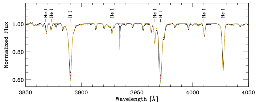
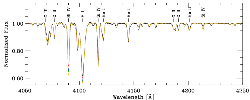
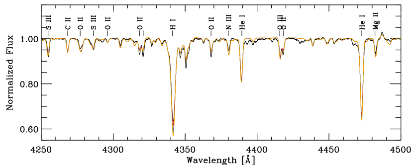
Figure A.21: Best model fits for $\epsilon$ Ori for each $f_{\infty}$ value: 1.0 (red), 0.1 (blue), 0.05 (green) and 0.01 (orange). Optical data are shown by the black line.

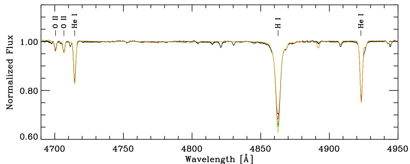
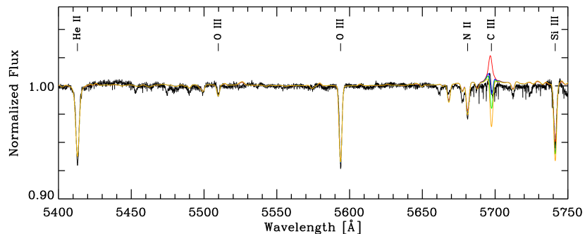
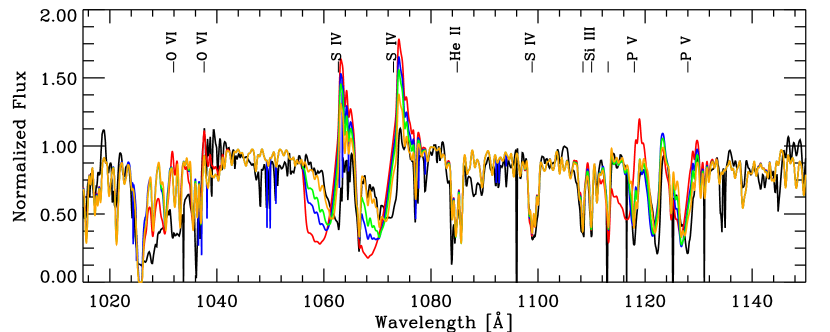
Figure A.22: Best model fits for $\epsilon$ Ori for each $f_{\infty}$ value: 1.0 (red), 0.1 (blue), 0.05 (green) and 0.01 (orange). Optical data are shown by the black line.

Figure A.23: Best model fits for $\epsilon$ Ori for each $f_{\infty}$ value: 1.0 (red), 0.1 (blue), 0.05 (green) and 0.01 (orange). Optical data are shown by the black line.

Figure A.24: Best model fits for $\epsilon$ Ori for each $f_{\infty}$ value: 1.0 (red), 0.1 (blue), 0.05 (green) and 0.01 (orange). The black line represents the COPERNICUS data. The influence of the inter clump medium on O vi $\lambda\lambda$1032,1038 has not been included.

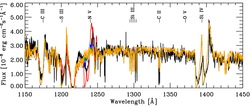
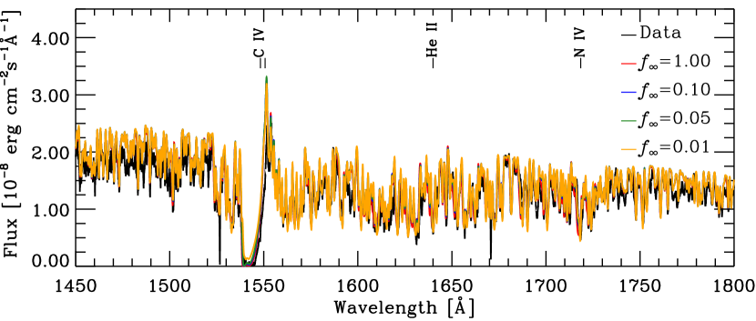
Figure A.25: Best model fits for $\epsilon$ Ori for each $f_{\infty}$ value: 1.0 (red), 0.1 (blue), 0.05 (green) and 0.01 (orange). The black line represents the IUE data. The influence of the inter clump medium on N v $\lambda\lambda$1238,1242 has not been included.

References

- Arnaud (1996) Arnaud K. A., 1996, in Jacoby G. H., Barnes J., eds, Astronomical Society of the Pacific Conference Series Vol. 101, Astronomical Data Analysis Software and Systems V. p. 17
- Asplund et al. (2009) Asplund M., Grevesse N., Sauval A. J., Scott P., 2009, ARA&A, 47, 481
- Auer & Mihalas (1972) Auer L. H., Mihalas D., 1972, ApJS, 24, 193
- Bagnulo et al. (2009) Bagnulo S., Landolfi M., Landstreet J. D., Landi Degl’Innocenti E., Fossati L., Sterzik M., 2009, PASP, 121, 993
- Blomme et al. (2002) Blomme R., Prinja R. K., Runacres M. C., Colley S., 2002, A&A, 382, 921
- Bouret et al. (2003) Bouret J.-C., Lanz T., Hillier D. J., Heap S. R., Hubeny I., Lennon D. J., Smith L. J., Evans C. J., 2003, ApJ, 595, 1182
- Bouret et al. (2005) Bouret J.-C., Lanz T., Hillier D. J., 2005, A&A, 438, 301
- Bouret et al. (2012) Bouret J.-C., Hillier D. J., Lanz T., Fullerton A. W., 2012, A&A, 544, A67
- Bouret et al. (2013) Bouret J.-C., Lanz T., Martins F., Marcolino W. L. F., Hillier D. J., Depagne E., Hubeny I., 2013, A&A, 555, A1
- Brown et al. (1994) Brown A. G. A., de Geus E. J., de Zeeuw P. T., 1994, A&A, 289, 101
- Busche & Hillier (2005) Busche J. R., Hillier D. J., 2005, AJ, 129, 454
- Cash (1979) Cash W., 1979, ApJ, 228, 939
- Cassinelli & Olson (1979) Cassinelli J. P., Olson G. L., 1979, ApJ, 229, 304
- Chiosi & Maeder (1986) Chiosi C., Maeder A., 1986, ARA&A, 24, 329
- Cohen et al. (2010) Cohen D. H., Leutenegger M. A., Wollman E. E., Zsargó J., Hillier D. J., Townsend R. H. D., Owocki S. P., 2010, MNRAS, 405, 2391
- Cohen et al. (2011) Cohen D. H., Gagné M., Leutenegger M. A., MacArthur J. P., Wollman E. E., Sundqvist J. O., Fullerton A. W., Owocki S. P., 2011, MNRAS, 415, 3354
- Cohen et al. (2014a) Cohen D. H., Wollman E. E., Leutenegger M. A., Sundqvist J. O., Fullerton A. W., Zsargó J., Owocki S. P., 2014a, MNRAS, 439, 908
- Cohen et al. (2014b) Cohen D. H., Li Z., Gayley K. G., Owocki S. P., Sundqvist J. O., Petit V., Leutenegger M. A., 2014b, MNRAS, 444, 3729
- Crowther et al. (2002) Crowther P. A., Hillier D. J., Evans C. J., Fullerton A. W., De Marco O., Willis A. J., 2002, ApJ, 579, 774
- Crowther et al. (2006) Crowther P. A., Lennon D. J., Walborn N. R., 2006, A&A, 446, 279
- Cunha et al. (2006) Cunha K., Hubeny I., Lanz T., 2006, ApJ, 647, L143
- Dessart & Owocki (2003) Dessart L., Owocki S. P., 2003, A&A, 406, L1
- Dessart & Owocki (2005) Dessart L., Owocki S. P., 2005, A&A, 437, 657
- Diplas & Savage (1994) Diplas A., Savage B. D., 1994, ApJS, 93, 211
- Drake & Testa (2005) Drake J. J., Testa P., 2005, Nature, 436, 525
- Ebbets (1982) Ebbets D., 1982, ApJS, 48, 399
- Evans (1967) Evans D. S., 1967, in Batten A. H., Heard J. F., eds, IAU Symposium Vol. 30, Determination of Radial Velocities and their Applications. p. 57
- Evans et al. (2004) Evans C. J., Crowther P. A., Fullerton A. W., Hillier D. J., 2004, ApJ, 610, 1021
- Eversberg et al. (1998) Eversberg T., Lépine S., Moffat A. F. J., 1998, ApJ, 494, 799
- Feldmeier et al. (1997) Feldmeier A., Puls J., Pauldrach A. W. A., 1997, A&A, 322, 878
- Foster et al. (2012) Foster A. R., Ji L., Smith R. K., Brickhouse N. S., 2012, ApJ, 756, 128
- Fullerton et al. (1996) Fullerton A. W., Gies D. R., Bolton C. T., 1996, ApJS, 103, 475
- Fullerton et al. (2006) Fullerton A. W., Massa D. L., Prinja R. K., 2006, ApJ, 637, 1025
- Fullerton et al. (2008) Fullerton A. W., Massa D. L., Prinja R. K., 2008, in Hamann W.-R., Feldmeier A., Oskinova L. M., eds, Clumping in Hot-Star Winds. p. 23
- Gabriel & Jordan (1969) Gabriel A. H., Jordan C., 1969, MNRAS, 145, 241
- Gray (2008) Gray D. F., 2008, The Observation and Analysis of Stellar Photospheres. Cambridge University Press, 2008
- Harnden et al. (1979) Harnden Jr. F. R., et al., 1979, ApJ, 234, L51
- Hearn (1975) Hearn A. G., 1975, A&A, 40, 355
- Hervé et al. (2013) Hervé A., Rauw G., Nazé Y., 2013, A&A, 551, A83
- Hillier (1991) Hillier D. J., 1991, A&A, 247, 455
- Hillier (2003) Hillier D. J., 2003, in I. Hubeny, D. Mihalas, & K. Werner ed., Astronomical Society of the Pacific Conference Series Vol. 288, Stellar Atmosphere Modeling. pp 199–+
- Hillier & Miller (1998) Hillier D. J., Miller D. L., 1998, ApJ, 496, 407
- Hillier & Miller (1999) Hillier D. J., Miller D. L., 1999, ApJ, 519, 354
- Hillier et al. (2012) Hillier D. J., Bouret J.-C., Lanz T., Busche J. R., 2012, MNRAS, 426, 1043
- Howarth & Lamers (1999) Howarth I., Lamers H. J. G., 1999, Journal of the British Astronomical Association, 109, 347
- Howarth et al. (1997) Howarth I. D., Siebert K. W., Hussain G. A. J., Prinja R. K., 1997, MNRAS, 284, 265
- Ignace & Gayley (2002) Ignace R., Gayley K. G., 2002, ApJ, 568, 954
- Kaper et al. (1996) Kaper L., Henrichs H. F., Nichols J. S., Snoek L. C., Volten H., Zwarthoed G. A. A., 1996, A&AS, 116, 257
- Knobel (1909) Knobel E. B., 1909, The Observatory, 32, 357
- Krtička & Kubát (2009) Krtička J., Kubát J., 2009, MNRAS, 394, 2065
- Krtička & Kubát (2012) Krtička J., Kubát J., 2012, MNRAS, 427, 84
- Kudritzki et al. (1999) Kudritzki R. P., Puls J., Lennon D. J., Venn K. A., Reetz J., Najarro F., McCarthy J. K., Herrero A., 1999, A&A, 350, 970
- Lamers (1974) Lamers H. J. G. L. M., 1974, A&A, 37, 237
- Lamers & Leitherer (1993) Lamers H. J. G. L. M., Leitherer C., 1993, ApJ, 412, 771
- Lee (1968) Lee T. A., 1968, ApJ, 152, 913
- Lesh (1968) Lesh J. R., 1968, ApJS, 17, 371
- Leutenegger et al. (2006) Leutenegger M. A., Paerels F. B. S., Kahn S. M., Cohen D. H., 2006, ApJ, 650, 1096
- Leutenegger et al. (2007) Leutenegger M. A., Owocki S. P., Kahn S. M., Paerels F. B. S., 2007, ApJ, 659, 642
- Leutenegger et al. (2010) Leutenegger M. A., Cohen D. H., Zsargó J., Martell E. M., MacArthur J. P., Owocki S. P., Gagné M., Hillier D. J., 2010, ApJ, 719, 1767
- Leutenegger et al. (2013) Leutenegger M. A., Cohen D. H., Sundqvist J. O., Owocki S. P., 2013, ApJ, 770, 80
- Lucy (1982) Lucy L. B., 1982, ApJ, 255, 286
- Lucy (2010) Lucy L. B., 2010, A&A, 524, A41
- Lucy & White (1980) Lucy L. B., White R. L., 1980, ApJ, 241, 300
- Macfarlane et al. (1991) Macfarlane J. J., Cassinelli J. P., Welsh B. Y., Vedder P. W., Vallerga J. V., Waldron W. L., 1991, ApJ, 380, 564
- Macfarlane et al. (1994) Macfarlane J. J., Cohen D. H., Wang P., 1994, ApJ, 437, 351
- Maeder & Meynet (2000) Maeder A., Meynet G., 2000, ARA&A, 38, 143
- Marcolino et al. (2009) Marcolino W. L. F., Bouret J.-C., Martins F., Hillier D. J., Lanz T., Escolano C., 2009, A&A, 498, 837
- Martins & Hillier (2012) Martins F., Hillier D. J., 2012, A&A, 545, A95
- Martins et al. (2005) Martins F., Schaerer D., Hillier D. J., Meynadier F., Heydari-Malayeri M., Walborn N. R., 2005, A&A, 441, 735
- Martins et al. (2015) Martins F., Marcolino W., Hillier D. J., Donati J.-F., Bouret J.-C., 2015, A&A, 574, A142
- McErlean et al. (1998) McErlean N. D., Lennon D. J., Dufton P. L., 1998, A&A, 329, 613
- McErlean et al. (1999) McErlean N. D., Lennon D. J., Dufton P. L., 1999, A&A, 349, 553
- Morel et al. (2004) Morel T., Marchenko S. V., Pati A. K., Kuppuswamy K., Carini M. T., Wood E., Zimmerman R., 2004, MNRAS, 351, 552
- Najarro et al. (2006) Najarro F., Hillier D. J., Puls J., Lanz T., Martins F., 2006, A&A, 456, 659
- Najarro et al. (2011) Najarro F., Hanson M. M., Puls J., 2011, A&A, 535, A32
- Nieva & Przybilla (2006) Nieva M. F., Przybilla N., 2006, ApJ, 639, L39
- Oskinova et al. (2006) Oskinova L. M., Feldmeier A., Hamann W.-R., 2006, MNRAS, 372, 313
- Oskinova et al. (2007) Oskinova L. M., Hamann W.-R., Feldmeier A., 2007, A&A, 476, 1331
- Oskinova et al. (2011) Oskinova L., Hamann W.-R., Ignace R., Feldmeier A., 2011, Bulletin de la Societe Royale des Sciences de Liege, 80, 54
- Owocki (2008) Owocki S. P., 2008, in Hamann W.-R., Feldmeier A., Oskinova L. M., eds, Clumping in Hot-Star Winds. p. 121
- Owocki & Cohen (2001) Owocki S. P., Cohen D. H., 2001, ApJ, 559, 1108
- Owocki & Cohen (2006) Owocki S. P., Cohen D. H., 2006, ApJ, 648, 565
- Owocki et al. (1988) Owocki S. P., Castor J. I., Rybicki G. B., 1988, ApJ, 335, 914
- Perryman et al. (1997) Perryman M. A. C., et al., 1997, A&A, 323, L49
- Petit et al. (2014) Petit P., Louge T., Théado S., Paletou F., Manset N., Morin J., Marsden S. C., Jeffers S. V., 2014, PASP, 126, 469
- Petrov et al. (2014) Petrov B., Vink J. S., Gräfener G., 2014, A&A, 565, A62
- Porquet et al. (2001) Porquet D., Mewe R., Dubau J., Raassen A. J. J., Kaastra J. S., 2001, A&A, 376, 1113
- Prinja & Massa (2010) Prinja R. K., Massa D. L., 2010, A&A, 521, L55
- Prinja et al. (2002) Prinja R. K., Massa D., Fullerton A. W., 2002, A&A, 388, 587
- Prinja et al. (2004) Prinja R. K., Rivinius T., Stahl O., Kaufer A., Foing B. H., Cami J., Orlando S., 2004, A&A, 418, 727
- Prinja et al. (2006) Prinja R. K., Markova N., Scuderi S., Markov H., 2006, A&A, 457, 987
- Puls et al. (2005) Puls J., Urbaneja M. A., Venero R., Repolust T., Springmann U., Jokuthy A., Mokiem M. R., 2005, A&A, 435, 669
- Puls et al. (2006) Puls J., Markova N., Scuderi S., Stanghellini C., Taranova O. G., Burnley A. W., Howarth I. D., 2006, A&A, 454, 625
- Repolust et al. (2005) Repolust T., Puls J., Hanson M. M., Kudritzki R.-P., Mokiem M. R., 2005, A&A, 440, 261
- Rivero González et al. (2011) Rivero González J. G., Puls J., Najarro F., 2011, A&A, 536, A58
- Rivero González et al. (2012a) Rivero González J. G., Puls J., Najarro F., Brott I., 2012a, A&A, 537, A79
- Rivero González et al. (2012b) Rivero González J. G., Puls J., Massey P., Najarro F., 2012b, A&A, 543, A95
- Runacres & Owocki (2002) Runacres M. C., Owocki S. P., 2002, A&A, 381, 1015
- Santolaya-Rey et al. (1997) Santolaya-Rey A. E., Puls J., Herrero A., 1997, A&A, 323, 488
- Savage et al. (1977) Savage B. D., Bohlin R. C., Drake J. F., Budich W., 1977, ApJ, 216, 291
- Searle et al. (2008) Searle S. C., Prinja R. K., Massa D., Ryans R., 2008, A&A, 481, 777
- Seward et al. (1979) Seward F. D., Forman W. R., Giacconi R., Griffiths R. E., Harnden Jr. F. R., Jones C., Pye J. P., 1979, ApJ, 234, L55
- Silvester et al. (2012) Silvester J., Wade G. A., Kochukhov O., Bagnulo S., Folsom C. P., Hanes D., 2012, MNRAS, 426, 1003
- Simón-Díaz & Herrero (2007) Simón-Díaz S., Herrero A., 2007, A&A, 468, 1063
- Smith et al. (2001) Smith R. K., Brickhouse N. S., Liedahl D. A., Raymond J. C., 2001, ApJ, 556, L91
- Snow & Morton (1976) Snow Jr. T. P., Morton D. C., 1976, ApJS, 32, 429
- Sundqvist et al. (2010) Sundqvist J. O., Puls J., Feldmeier A., 2010, A&A, 510, A11
- Sundqvist et al. (2011) Sundqvist J. O., Puls J., Feldmeier A., Owocki S. P., 2011, A&A, 528, A64
- Sundqvist et al. (2012) Sundqvist J. O., Owocki S. P., Cohen D. H., Leutenegger M. A., Townsend R. H. D., 2012, MNRAS, 420, 1553
- Sundqvist et al. (2014) Sundqvist J. O., Puls J., Owocki S. P., 2014, A&A, 568, A59
- Thompson & Morrison (2013) Thompson G. B., Morrison N. D., 2013, AJ, 145, 95
- Trundle & Lennon (2005) Trundle C., Lennon D. J., 2005, A&A, 434, 677
- Trundle et al. (2004) Trundle C., Lennon D. J., Puls J., Dufton P. L., 2004, A&A, 417, 217
- Urbaneja (2004) Urbaneja M., 2004, PhD thesis, University of La Laguna
- Verner & Yakovlev (1995) Verner D. A., Yakovlev D. G., 1995, A&AS, 109, 125
- Vink et al. (2000) Vink J. S., de Koter A., Lamers H. J. G. L. M., 2000, A&A, 362, 295
- Vink et al. (2001) Vink J. S., de Koter A., Lamers H. J. G. L. M., 2001, A&A, 369, 574
- Walborn (1976) Walborn N. R., 1976, ApJ, 205, 419