Full-density multi-scale account of structure and dynamics of macaque visual cortex

Maximilian Schmidt¹, Rembrandt Bakker^1,2, Kelly Shen³, Gleb Bezgin⁴, Claus-Christian Hilgetag^5,6, Markus Diesmann^1,7,8, and Sacha Jennifer van Albada¹

¹ Institute of Neuroscience and Medicine (INM-6) and Institute for Advanced Simulation (IAS-6) and JARA BRAIN Institute I, Jülich Research Centre, Jülich, Germany

² Donders Institute for Brain, Cognition and Behavior, Radboud University Nijmegen, Netherlands

³ Rotman Research Institute, Baycrest, Toronto, Ontario M6A 2E1, Canada

⁴ McConnell Brain Imaging Centre, Montreal Neurological Institute, McGill University, Montreal, Canada

⁵ Department of Computational Neuroscience, University Medical Center Eppendorf, Hamburg, Germany

⁶ Department of Health Sciences, Boston University, USA

⁷ Department of Psychiatry, Psychotherapy and Psychosomatics, Medical Faculty, RWTH Aachen University, Aachen, Germany

⁸ Department of Physics, Faculty 1, RWTH Aachen University, Aachen, Germany

^∗Correspondence to:    Maximilian Schmidt Forschungszentrum Jülich 52425 Jülich, Germany max.schmidt@fz-juelich.de

Abstract

We present a multi-scale spiking network model of all vision-related areas of macaque cortex that represents each area by a full-scale microcircuit with area-specific architecture. The layer- and population-resolved network connectivity integrates axonal tracing data from the CoCoMac database with recent quantitative tracing data, and is systematically refined using dynamical constraints. Simulations reveal a stable asynchronous irregular ground state with heterogeneous activity across areas, layers, and populations. Elicited by large-scale interactions, the model reproduces longer intrinsic time scales in higher compared to early visual areas. Activity propagates down the visual hierarchy, similar to experimental results associated with visual imagery. Cortico-cortical interaction patterns agree well with fMRI resting-state functional connectivity. The model bridges the gap between local and large-scale accounts of cortex, and clarifies how the detailed connectivity of cortex shapes its dynamics on multiple scales.

Introduction

Cortical activity has distinct but interdependent features on local and global scales, molded by connectivity on each scale. Globally, resting-state activity has characteristic patterns of correlations (Vincent et al., 2007; Fox & Raichle, 2007; Shen et al., 2012) and propagation (Mitra et al., 2014) between areas. Locally, neurons spike with time scales that tend to increase from sensory to prefrontal areas (Murray et al., 2014) in a manner influenced by both short-range and long-range connectivity (Chaudhuri et al., 2015). We present a full-density multi-scale spiking network model in which these features arise naturally from its detailed structure.

Models of cortex have hitherto used two basic approaches. The first models each neuron explicitly in networks ranging from local microcircuits to small numbers of connected areas (Hill & Tononi, 2005; Haeusler et al., 2009). The second represents the large-scale dynamics of cortex by simplifying the ensemble dynamics of areas or populations to few differential equations, such as Wilson-Cowan or Kuramoto oscillators (Deco et al., 2009; Cabral et al., 2011). These models can for instance reproduce resting-state oscillations at $\sim\!0.1\,\mathrm{Hz}$. Chaudhuri et al. (2015) developed a mean-field multi-area model with a hierarchy of intrinsic time scales in the population firing rates, relying on a gradient of excitation across areas.

Cortical processing is not restricted to one or few areas, but results from complex interactions between many areas involving feedforward and feedback processes (Lamme et al., 1998; Rao & Ballard, 1999). At the same time, the high degree of connectivity within areas (Angelucci et al., 2002a; Markov et al., 2011) hints at the importance of local processing. Capturing both aspects requires multi-scale models that combine the detailed features of local microcircuits with realistic inter-area connectivity. Another advantage of multi-scale modeling is that it enables testing the equivalence between population models and models at cellular resolution instead of assuming it a priori.

Two main obstacles of multi-scale simulations are now gradually being overcome. First, such simulations require large resources on high-performance clusters or supercomputers and simulation technology that uses these resources efficiently. Recently, important technological progress has been achieved for the NEST simulator (Kunkel et al., 2014). Second, gaps in anatomical knowledge have prevented the consistent definition of multi-area models. Recent developments in the CoCoMac database (Bakker et al., 2012) and quantitative axonal tracing (Markov et al., 2014a, b) have systematized connectivity data for macaque cortex. However, it remains necessary to use statistical regularities such as relationships between architectural differentiation and connectivity (Barbas, 1986; Barbas & Rempel-Clower, 1997) to fully specify large cortical network models. Because of these difficulties, few large-scale spiking network models have been simulated to date, and existing ones heavily downscale the number of synapses per neuron (Izhikevich & Edelman, 2008; Preissl et al., 2012), generally affecting network dynamics (van Albada et al., 2015).

We here use realistic numbers of synapses per neuron, building on a recent model of a $1\>\mathrm{mm}^{2}$ cortical microcircuit with $\sim\!10^{5}$ neurons (Potjans & Diesmann, 2014). This is the smallest network size where the majority of inputs per neuron ($\sim\!10,\!000$) is self-consistently represented at realistic connectivity ($\sim\!10\%$). Nonetheless, a substantial fraction of synapses originates outside the microcircuit and is replaced by stochastic input. Our model reduces random input by including all vision-related areas.

The model combines simple single-neuron dynamics with complex connectivity and thereby allows us to study the influence of the connectivity itself on the network dynamics. The connectivity map customizes that of the microcircuit model to each area based on its architecture and adds inter-areal connections. By a mean-field method (Schuecker et al., 2015), we refine the connectivity to fulfill the basic dynamical constraint of nonzero and non-saturated activity.

The ground state of cortex features asynchronous irregular spiking with low pairwise correlations (Ecker et al., 2010) and low spike rates $(\sim\!0.1-30\;\mathrm{spikes}/\mathrm{s})$ with inhibitory cells spiking faster than excitatory ones (Swadlow, 1988). Our model reproduces each of these phenomena, bridging the gap between local and global brain models, and relating the complex structure of cortex to its spiking dynamics.

Results

The model comprises 32 areas of macaque cortex involved in visual processing in the parcellation of Felleman & Van Essen (1991), henceforth referred to as FV91 (Table S1). Each area contains an excitatory and an inhibitory population in each of the layers 2/3, 4, 5 and 6 (L2/3, L4, L5, L6), except area TH, which lacks L4. The model, summarized in Table 1, represents each area by a $1\>\mathrm{mm}^{2}$ patch.

Area-specific laminar compositions

Neuronal volume densities provided in a different parcellation scheme are mapped to the FV91 scheme and partly estimated using the average density of each layer across areas of the same architectural type (Figure 1A). Architectural types (Table 4 of Hilgetag et al., 2015) reflect the distinctiveness of the lamination as well as L4 thickness, with agranular cortices having the lowest and V1 the highest value. Neuron density increases with architectural type. When referring to architectural types, we also use the term ‘structural hierarchy’. We call areas like V1 and V2 at the bottom of the structural (or processing) hierarchy ‘early’, and those near the top ‘higher’ areas.

We find total cortical thicknesses of 14 areas to decrease with logarithmized overall neuron densities, enabling us to estimate the total thicknesses of the other $18$ areas (Figure 1B). Quantitative data from the literature combined with our own estimates from published micrographs (Table S5) determine laminar thicknesses (Figure 1C). L4 thickness relative to total cortical thickness increases with the logarithm of overall neuron density, which predicts relative L4 thickness for areas with missing data. Since the relative thicknesses of the other layers show no notable change with architectural type, we fill in missing values using the mean of the known data for these quantities and then normalize the sum of the relative thicknesses to $1$. Layer thicknesses then follow from relative thickness times total thickness (see Table S6).

Finally, for lack of more specific data, the proportions of excitatory and inhibitory neurons in each layer are taken from cat V1 (Binzegger et al., 2004). Multiplying these with the laminar thicknesses and neuron densities yields the population sizes (see Experimental procedures).

Each neuron receives synapses of four different origins (Figure 1D). In the following, we describe how the counts for these synapse types are computed (details in Experimental procedures).

Scalable scheme of local connectivity

We assume constant synaptic volume density across areas (Harrison et al., 2002). Experimental values for the average indegree in monkey visual cortex vary between $2,\!300$ (O’Kusky & Colonnier, 1982) and $5,\!600$ (Cragg, 1967) synapses per neuron. We take the average ($3,\!950$) as representative for V1, resulting in a synaptic density of $8.3\cdot 10^{8}\>\frac{\textrm{synapses}}{\textrm{mm}^{3}}$.

The microcircuit model of Potjans & Diesmann (2014) serves as a prototype for all areas. The indegrees are a defining characteristic of this local circuit, as they govern the mean synaptic currents. We thus preserve their relative values when customizing the microcircuit to area-specific neuron densities and laminar thicknesses. The connectivity between populations is spatially uniform. The connection probability averages an underlying Gaussian connection profile over a disk with the surface area of the simulated area, separating simulated local synapses (type I) formed within the disk from non-simulated local synapses (type II) from outside the disk (Figure 1D, E). In retrograde tracing experiments, Markov et al. (2011) found the fraction of labeled neurons intrinsic to each injected area ($FLN_{\mathrm{i}}$) to be approximately constant, with a mean of $0.79$. We translate this to numbers of synapses by assuming that the proportion of synapses of type I is $0.79$ for realistic area size. For the $1\>\mathrm{mm}^{2}$ model areas, we obtain an average proportion of type I synapses of $0.504$.

Layer-specific heterogeneous cortico-cortical connectivity

We treat all cortico-cortical connections as originating and terminating in the $1\>\mathrm{mm}^{2}$ patches, ignoring their spatial divergence and convergence. Two areas are connected if the connection is in CoCoMac (Figure 1F) or reported by Markov et al. (2014a). For the latter we assume that the average number of synapses per labeled neuron is constant across projecting areas (Figure 1G). To estimate missing values, we exploit the exponential decay of connectivity with distance (Ercsey-Ravasz et al., 2013). We first map the data from its native parcellation scheme (M132) to the FV91 scheme (see Experimental procedures) and then perform a least-squares fit (Figure 1H). Combining the binary information on the existence of connections with the connection densities gives the area-level connectivity matrix (Figure 1I).

Next, we distribute synapses between the populations of each pair of areas (Figure 1K). The pattern of source layers is based on CoCoMac, if laminar data is available. Fractions of supragranular labeled neurons ($SLN$) from retrograde tracing experiments yield proportions of projecting neurons in supra- and infragranular layers (Markov et al., 2014b). To predict missing values, we exploit a sigmoidal relation between the logarithmized ratios of cell densities of the participating areas and the $SLN$ of their connection (as suggested by Beul et al. 2015; Figure 1J). Following Markov et al. (2014b), we use a generalized linear model for the fit and assume a beta-binomial distribution of source neurons. Since Markov et al. (2014b) do not distinguish infragranular layers further into L5 and L6, we use the more detailed laminar patterns from CoCoMac for this purpose, if available. We exclude L4 from the source patterns, in line with anatomical observations (Felleman & Van Essen, 1991), and approximate cortico-cortical connections as purely excitatory (Salin & Bullier, 1995; Tomioka & Rockland, 2007).

We base termination patterns on anterograde tracing studies collected in CoCoMac, if available, or on a relationship between source and target patterns (see Experimental procedures). Since neurons can receive synapses in different layers on their dendritic branches, we use laminar profiles of reconstructed cell morphologies (Binzegger et al., 2004) to relate synapse to cell-body locations. Despite the use of a point neuron model, we thus take into account the layer specificity of synapses on the single-cell level. In contrast to laminar synapse distributions, the resulting laminar distributions of target cell bodies are not highly distinct between feedforward and feedback projections.

Brain embedding

Inputs from outside the scope of our model, i.e., white-matter inputs from non-cortical or non-visual cortical areas and gray-matter inputs from outside the $1\,\mathrm{mm^{2}}$ patch, are represented by Poisson spike trains. Corresponding numbers of synapses are not available for all areas, and laminar patterns of external inputs differ between target areas (Felleman & Van Essen, 1991; Markov et al., 2014b). Therefore, we determine the total number of external synapses onto an area as the total number of synapses minus those of type I and III, and distribute them with equal indegree for all populations.

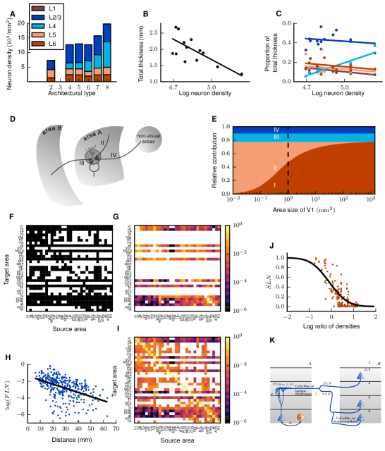
Figure 1: Construction principles of the model. (A) Laminar neuron densities for the architectural types in the model. Type 2, here corresponding only to area TH, lacks L4. In the model, L1 contains synapses but no neurons. Data provided by H. Barbas and C. Hilgetag (personal communication) and linearly scaled up to account for undersampling of cells by NeuN staining relative to Nissl staining as determined by repeat measurements of 11 areas. (B) Total thickness vs. logarithmized overall neuron density and linear least-squares fit ($r=-0.7,\>p=0.005$). (C) Relative laminar thickness (see Table S5) vs. logarithmized overall neuron density and linear least-squares fits (L1: $r=-0.51,\,p=0.08$, L2/3: $r=-0.20,\,p=0.52$, L4: $r=0.89,\>p=0.0001$; L5: $r=-0.31,\>p=0.36$, L6: $r=-0.26,\,p=0.43$). Total cortical thicknesses $D(A)$ and overall neuron densities for $14$ areas provided by H. Barbas and C. Hilgetag (personal communication), measured by Nissl staining for the 11 areas mentioned above and for 3 areas by NeuN staining and linearly scaled up to account for undersampling. The data partially overlap with Hilgetag et al. (2015). (D) Scheme of the different types of connections to each neuron. I: Simulated intra-area synapses, II: Intra-area synapses from outside the $1\>\mathrm{mm}^{2}$ patch modeled as Poisson sources, III: Simulated cortico-cortical synapses, IV: Synapses from subcortical and non-visual cortical areas modeled as Poisson sources. (E) Relative contributions to indegrees in V1 for increasing cortical surface area covered by the model. Type I synapses increase at the cost of random input at type II synapses. Numbers of type III and IV synapses stay constant. The dashed line indicates the $1\>\mathrm{mm}^{2}$ surface area used here. (F) Binary connectivity from CoCoMac. Black, existing connections; white, absent connections. (G) Fractions of labeled neurons ($FLN$) from Markov et al. (2014a) mapped from their parcellation scheme (M132) to that of Felleman & Van Essen (1991). (H) Connection densities decay exponentially with inter-area distance. Black line, linear regression with $\log\left(FLN\right)=\log\left(C\right)-\lambda d$ ($C=0.045,\lambda=0.11,p=10^{-19}$; cf. (5)). (I) Area-level connectivity of the model, based on data in panels F-H, expressed as relative indegrees for each target area. (J) Fraction of source neurons in supragranular layers ($SLN$) vs. logarithmized ratio of the overall neuron densities of the two areas. $SLN$ from Markov et al. (2014b), neuron densities from Hilgetag et al. (2015). Black curve, fit using a beta-binomial generalized linear model (6) ($a_{0}=-0.152\text{, }a_{1}=-1.534\text{, }\phi=0.214$). (K) Illustration of the procedure for distributing synapses across layers. Source neuron $j$ from area $B$ sends an axon to layer $v$ of area $A$ where a cortico-cortical synapse $s_{\mathrm{CC}}$ is formed at the dendrite of neuron $i$. The procedure is detailed in Experimental procedures. See (9) for the formal definitions.

Refinement of connectivity by dynamical constraints

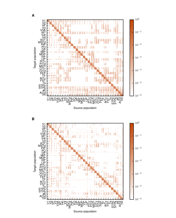
Figure S1: Related to Figure 1. Connection probabilities of the model encoded in color before (A) and after (B) applying the theoretical method described in Schuecker et al. (2015). Areas are ordered according to their architectural types, and populations inside the areas are ordered as [2/3E, 2/3I, 4E/, 4I, 5E, 5I, 6E, 6I].

Parameter scans based on mean-field theory (Schuecker et al., 2015) and simulations reveal a bistable activity landscape with two coexisting stable fixed points. The first has reasonable firing rates except for populations 5E and 6E, which are nearly silent (Figure 2A), while the second has excessive rates (Figure 2B) in almost all populations. Depending on the parameter configuration, either the low-activity fixed point has a sufficiently large basin of attraction for the simulated activity to remain near it, or fluctuations drive the network to the high-activity fixed point. To counter this shortcoming, we define an additional parameter $\kappa$ which increases the external drive onto 5E by a factor $\kappa=K_{\mathrm{ext,5E}}/K_{\mathrm{ext}}$ compared to the external drive of the other cell types. Since the rates in population 6E are even lower, we increase the external drive to 6E by a slightly larger factor than that to 5E. When applied directly to the model, even a small increase in $\kappa$ already drives the network into the undesired high-activity state (Figure 2B). Using the stabilization procedure described in Schuecker et al. (2015), we derive targeted modifications of the connectivity within the margins of uncertainty of the anatomical data, with an average relative change in total indegrees (summed over source populations) of $11.3\%$ (Figure S1B). This allows us to increase $\kappa$ while retaining the global stability of the low-activity state. In the following, we choose $\kappa=1.125$, which gives $K_{\mathrm{6E,\mathrm{ext}}}/K_{\mathrm{ext}}=1.417$ and the external inputs listed in Table S11, and $g=-11,\>\nu_{\mathrm{ext}}=10\;\mathrm{spikes}/\mathrm{s}$, yielding reasonable firing rates in populations 5E and 6E (Figure 2C). In total, the $4.13$ million neurons of the model are interconnected via $2.42\cdot 10^{10}$ synapses.

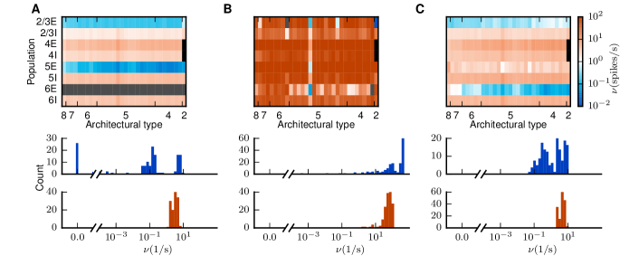
Figure 2: Attractors of the network. Top row: Firing rates of simulations with $g=-16$, $\nu_{\mathrm{ext}}=10\>\mathrm{spikes/s}$, $\kappa=1$ (A), $g=-16$, $\nu_{\mathrm{ext}}=10\>\mathrm{spikes/s}$, $\kappa=1.125$ (B), and $g=-11$, $\nu_{\mathrm{ext}}=10\>\mathrm{spikes/s}$, $\kappa=1.125$ with the modified connectivity matrix (C). The color bar holds for all three panels. Areas are ordered according to their architectural type along the horizontal axis from V1 (type 8) to TH (type 2) and populations are stacked vertically. The two missing populations 4E and 4I of area TH are marked in black and firing rates $<10^{-2}\>\mathrm{Hz}$ in gray. Bottom row: Histogram of population-averaged firing rates for excitatory (red) and inhibitory (blue) populations. The horizontal axis is split into linear- (left) and log-scaled (right) ranges.

The stabilization renders the intrinsic connectivity of the areas more heterogeneous. Cortico-cortical connection densities similarly undergo small changes, but with a notable reduction in the mutual connectivity between areas 46 and FEF. For more details on the connectivity changes, see Schuecker et al. (2015).

Community structure of anatomy relates to functional organization

We test if the stabilized network retains known organizing principles by analyzing the community structure in the weighted and directed graph of area-level connectivity. The map equation method (Rosvall et al., 2010) reveals 6 clusters (Figure 3). We test the significance of the corresponding modularity $Q=0.32$ by comparing with $1000$ surrogate networks conserving the total outdegree of each area by shuffling its targets. This yields $Q=-0.02\pm 0.03$, indicating the significance of our clustering. The community structure reflects anatomical and functional properties of the areas. Two large clusters comprise ventral and dorsal stream areas, respectively. Ventral area VOT is grouped with early visual area VP. Early sensory areas V1 and V2 form a separate cluster, as well as parahippocampal areas TH and TF. The two frontal areas FEF and 46 form the last cluster. Nonetheless, the clusters are heavily interconnected (Figure 3). The basic separation into ventral and dorsal clusters matches that found in the connection matrix of Felleman & Van Essen (1991) (Hilgetag et al., 2000) containing about half of the connections present in our weighted connectivity matrix, but there are also important differences. For instance, our clustering groups areas STPa, STPp, and 7a with the dorsal instead of the ventral stream, better matching the scheme described by Nassi & Callaway (2009).

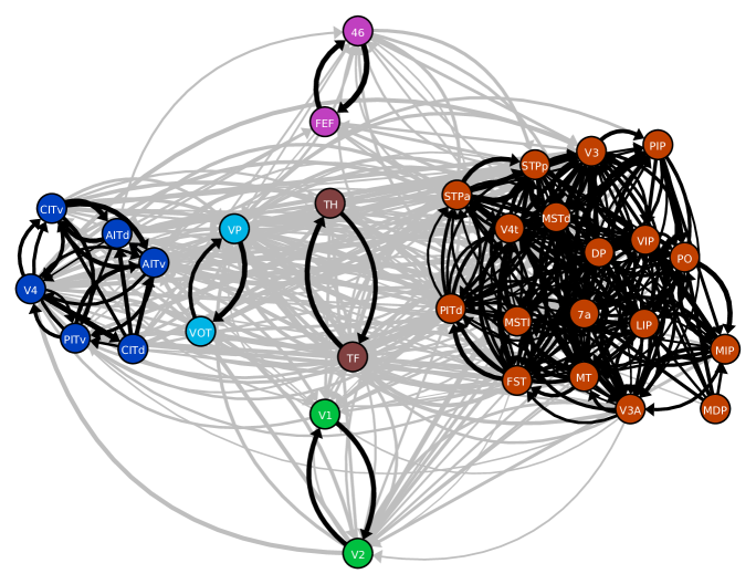
Figure 3: Community structure of the model. Clusters in the connectivity graph, indicated by the color of the nodes: Early visual areas (green), dorsal stream areas (red), areas VP and VOT (light blue), ventral stream (dark blue), parahippocampal areas (brown), and frontal areas (purple). Black, connections within clusters; gray, connections between clusters. Line thickness encodes logarithmized outdegrees. Only edges with relative outdegree$>10^{-3}$ are shown.

Area- and population-specific activity in the resting state

The model with cortico-cortical synaptic weights equal to local weights displays a reasonable ground state of activity but no substantial inter-area interactions (Figure S2). To control these interactions, we scale cortico-cortical synaptic weights $w_{\mathrm{cc}}$ onto excitatory neurons by a factor $\lambda=J_{\mathrm{cc}}^{\mathcal{E}}/J$ and provide balance by increasing the weights $J_{\mathrm{cc}}^{\mathrm{\mathcal{I}}}$ onto inhibitory neurons by twice this factor, $J_{\mathrm{cc}}^{\mathcal{I}}=\lambda_{\mathcal{I}}\lambda J=2\lambda J$. In the following, we choose $\lambda=1.9$. Simulations yield irregular activity with plausible firing rates (Figure 4A-C). Irregularly occurring population bursts of different lengths up to several seconds arise from the asynchronous baseline activity (Figure 4G) and propagate across the network. The firing rates differ across areas and layers and are generally low in L2/3 and L6 and higher in L4 and L5, partly due to the cortico-cortical interactions (Figure 4D). The overall average rate is $14.6\;\mathrm{spikes}/\mathrm{s}$. Inhibitory populations are generally more active than excitatory ones across layers and areas despite the identical intrinsic properties of the two cell types. However, the strong participation of L5E neurons in the cortico-cortical interaction bursts causes these to fire more rapidly than L5I neurons. Pairwise correlations are low throughout the network (Figure 4E). Excitatory neurons are more synchronized than inhibitory cells in the same layer, except for L6. Spiking irregularity is close to that of a Poisson process across areas and populations, with excitatory neurons consistently firing more irregularly than inhibitory cells (Figure 4F). Higher areas exhibit bursty spiking, as illustrated by the raster plot for area FEF (Figure 4C).

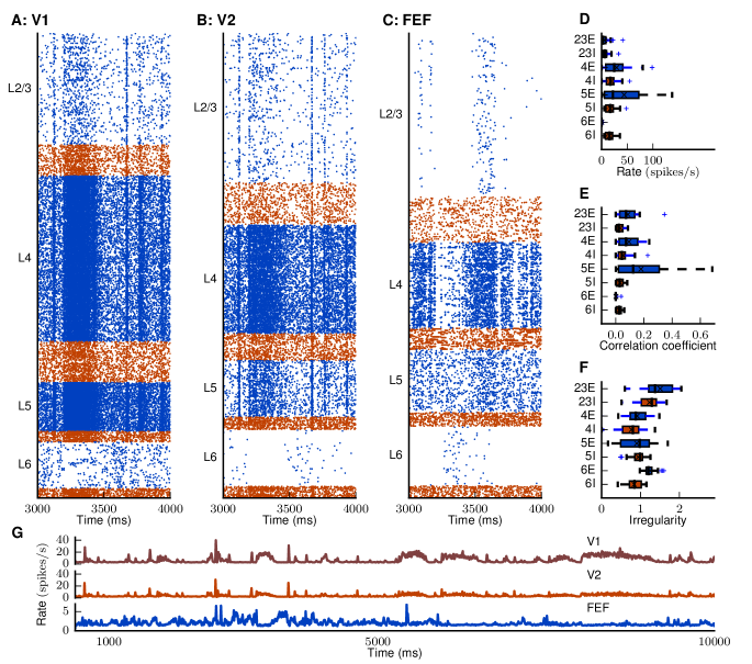
Figure 4: Resting state of the model. (A-C) Raster plot of spiking activity of $3\,\%$ of the neurons in area V1 (A), V2 (B), and FEF (C). (D-F) Spiking statistics across areas and populations shown as area-averaged box plots. (D) Population-averaged firing rates. (E) Average pairwise correlation coefficients of spiking activity. (F) Irregularity measured by revised local variation $LvR$ (Shinomoto et al., 2009) averaged across neurons. (G) Area-averaged firing rates.

Intrinsic time scales increase with structural hierarchy

We tested whether the model accounts for the hierarchical trend in intrinsic time scales observed in macaque cortex (Murray et al., 2014). Indeed, autocorrelation width in the model increases from early visual to higher areas. In early visual areas including V1, the autocorrelation decays with $\tau<2.5\>\mathrm{ms}$, indicating near-Poissonian spiking (Figure 5A). In higher areas, autocorrelations are broader with decay times $\sim\!10^{2}\>\mathrm{ms}$. The long time scales reflect bursty spike patterns of single-neuron activity (Figure 4), caused by the low neuron density in higher areas and thus high indegrees due to the constant synaptic density. A simulation with equal intrinsic and long-range synaptic weights that showed no significant interactions yielded near-Poissonian spiking in all areas (Figure S2), showing that the cortico-cortical interactions elicit the increased time scales. Area 46, which overlaps with lateral prefrontal cortex studied by Murray et al. (2014), shows a shorter time scale compared to the experimental data. However, in line with Murray et al. (2014), we find the time scale of area LIP to exceed that of MT, albeit by a small amount.

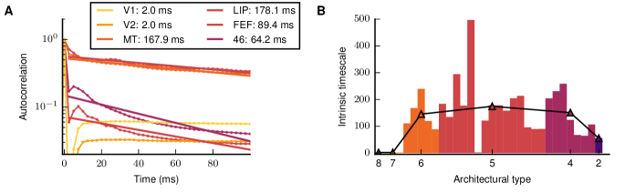
Figure 5: Intrinsic time scales. (A) Dots, autocorrelation function averaged across all populations in each area (colors in legend). Lines, exponential fit $f(t)=A\cdot\exp[-t/\tau]$. (B) Intrinsic time scales of areas vs. architectural type (color-coded). Average time scale per architectural type indicated by triangles and overall trend by black curve. Area MDP (architectural type 5) has a time scale of $2\>\mathrm{ms}$ because it is uncoupled from other areas due to the lack of incoming connections.

Structural and hierarchical directionality of spontaneous activity

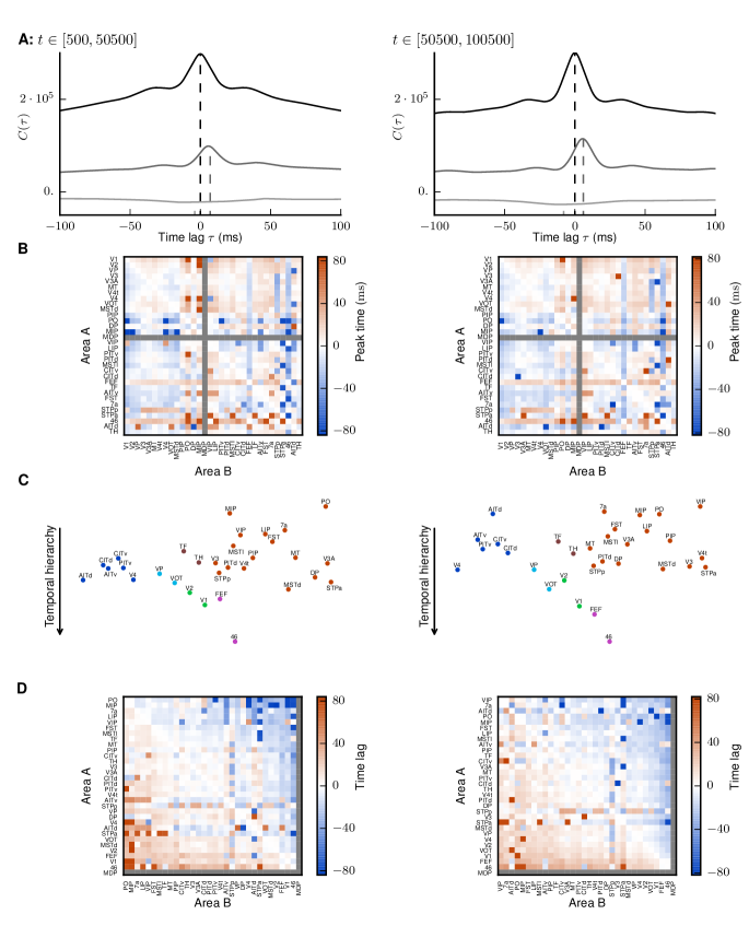
Figure S3: Related to Figure 6. Validation of the temporal hierarchy. Left column: First half of the time series ($t\in[500\>\mathrm{ms},\,50,500\>\mathrm{ms}]$), right column: second half of the time series ($t\in[50,500\>\mathrm{ms},\,100,500\>\mathrm{ms}]$). (A) Covariance functions of the area-averaged firing rates of V1 with areas V2 (gray) and FEF (light gray), and auto-covariance function of V1 (black). Dashed lines mark peak positions, detected by a wavelet smoothing algorithm (see Experimental procedures). (B) Matrix of peak positions of the correlation function for all pairs of areas. Area MDP was neglected because it has only outgoing but no incoming connections to other visual areas according to CoCoMac. (C) Temporal hierarchy. Colors indicate the cluster of each area found with the map equation algorithm (cf. Figure 3). Areas are horizontally arranged to avoid visual overlap. (D) Peak position matrix with areas in hierarchical order.

To investigate inter-area propagation, we determine the temporal order of spiking (Figure 6A) based on the correlation between areas. We detect the location of the extremum of the correlation function for each pair of areas (Figure 6B) and collect the corresponding time lags in a matrix (Figure 6C). In analogy to structural hierarchies based on pairwise connection patterns (Reid et al., 2009), we look for a temporal hierarchy that best reflects the order of activations for all pairs of areas (see Experimental procedures). The result (Figure 6D) places parietal and temporal areas at the beginning and early visual as well as frontal areas at the end. The first and second halves of the time series yield qualitatively identical results (Figure S3). Figure 6E shows the consistency of the hierarchy with the pairwise lags. To quantify the goodness of the hierarchy, we counted the pairs of areas for which it indicates a wrong ordering. The number of such violations is $190$ out of $496$, well below the $230\pm 12\,\text{(SD)}$ violations obtained for $100$ surrogate matrices, created by shuffling the entries of the original matrix while preserving its antisymmetric character. This indicates that the simulated temporal hierarchy reflects nonrandom patterns. The propagation is mostly in the feedback direction not only in terms of the structural hierarchy, but also spatially: activity starts in parietal regions, and spreads to the temporal and occipital lobes (Figure 6F). However, activity troughs in frontal areas follow peaks in occipital activity and thus appear last.

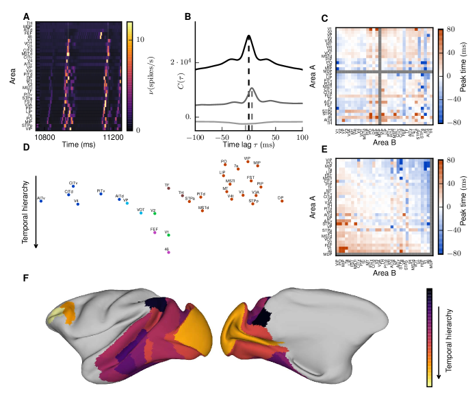
Figure 6: Temporal hierarchy. (A) Area-averaged firing rates for a sample period, with areas ordered according to the onset of increased activity from $t>1250\>\mathrm{ms}$. (B) Covariance functions of the area-averaged firing rates of V1 with areas V2 (gray) and FEF (light gray), and auto-covariance function of V1 (black). Dashed lines mark selected time lags, detected by a wavelet smoothing algorithm (see Experimental procedures). (C) Matrix of time lags of the correlation function for all pairs of areas. Area MDP was neglected because it has only outgoing connections to but no incoming connections from other visual areas according to CoCoMac. (D) Temporal hierarchy. Colors correspond to the map equation clustering (cf. Figure 3). Areas are horizontally arranged to avoid visual overlap. (E) Peak position matrix with areas in hierarchical order. (F) Lateral (left) and medial (right) view on the left hemisphere of an inflated macaque cortical surface showing the order in which areas are preferentially activated. Created with the “view/map 3d surface” tool on %****␣results.tex␣Line␣400␣****http://scalablebrainatlas.incf.org.

Emerging interactions mimic experimental functional connectivity

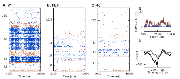
Figure S4: Related to Figure 7. Anticorrelation between V1 and frontal areas. (A-C) Raster plot of spiking activity of $0.1\,\%$ of the neurons in area V1 (A), FEF (B), and 46 (C). (D) Area-averaged firing rates of V1 (brown), FEF (red) and 46 (blue). (E) Covariance functions of the area-averaged firing rates of V1 with areas 46 (black) and FEF (gray). Parameters are the same as for the simulation used in Figure 7. The plot shows the anticorrelation between V1 and the two frontal areas visible in both the raster and the rate plot as well as in the negatively peaked cross-covariance function.

We compute the area-level functional connectivity (FC) based on the synaptic input current to each area, which has been shown to be more comparable to the BOLD fMRI than the spiking output (Logothetis et al., 2001). The FC matrix exhibits a rich structure, similar to experimental resting-state fMRI (Figure 7A, B, see Experimental procedures for details). In the simulation, frontal areas 46 and FEF are more weakly coupled with the rest of the network, but the anticorrelation with V1 is well captured by the model (Figure S4). Moreover, area MDP sends connections to, but does not receive connections from other areas according to CoCoMac, limiting its functional coupling to the network. Louvain clustering (Blondel et al., 2008), an algorithm optimizing the modularity of the weighted, undirected FC graph (Newman, 2004), yields two modules for both the simulated and the experimental data. The modules from the simulation differ from those of the structural connectivity and reflect the temporal hierarchy shown in Figure 6C. Cluster 1S merges early visual with ventral and two dorsal regions with average level in the temporal hierarchy of $\overline{h}=0.47\pm 0.13\,\text{(SD)}$. Cluster 2S contains mostly temporally earlier areas ($\overline{h}=0.33\pm 0.25\,\text{(SD)}$) merging parahippocampal with dorsal but also frontal areas. The experimental module 2E comprises only dorsal areas, while 1E consists of all other areas including also eight dorsal areas.

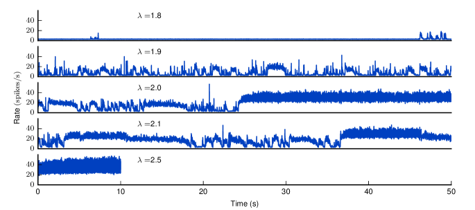
Figure S5: Related to Figure 7. Increasing cortico-cortical synaptic weights leads to switching to a high-activity state. Area-averaged firing rates in V1 for four different settings of $\lambda$. The simulation for $\lambda=2.5$ was run for $10\>\mathrm{s}$ biological time only. From$\lambda=2$ on, the network spontaneously enters a high-activity state. For $\lambda=2.5$, the network is in this state from the outset.

The structural connectivity of our model shows higher correlation with the experimental FC ($r_{\mathrm{Pearson}}=0.34$) than the binary connectivity matrices from both a previous (Shen et al., 2015) and the most recent release of CoCoMac ($r_{\mathrm{Pearson}}=0.20)$, further validating our weighted connectivity matrix. For increasing weight factor $\lambda$, the correlation between simulation and experiment improves (Figure 7D). For $\lambda=1$, areas interact weakly, resulting in low correlation between simulation and experiment (Figure S2). For intermediate cortico-cortical connection strengths, the correlation of simulation vs. experiment exceeds that between the structural connectivity and experimental FC (Figure 7C), indicating the enhanced explanatory power of the dynamical model. From $\lambda=2$ on, the network is prone to switch to the high-activity state (Figure S5). Thus, the highest correlation ($r_{\mathrm{Pearson}}=0.47$ for $\lambda=1.9$) occurs just below the onset of a state in which the model visits both the low-activity and high-activity attractors.

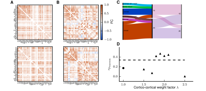
Figure 7: Inter-area interactions. (A) Simulated functional connectivity (FC) for $\lambda=1.9$ measured by the zero-time lag correlation coefficient of synaptic input currents. (B) FC from macaque resting-state fMRI (see Experimental procedures). Areas are ordered according to a clustering with the Louvain algorithm (Blondel et al., 2008) applied to the simulated data (top row) and to the experimental data (bottom row), respectively (see Experimental procedures). (C) Alluvial diagram showing the differences in the clusters for the structural connectivity (left), the simulated FC (center) and the experimentally measured FC (right). (D) Pearson correlation coefficient of simulated FC vs. experimentally measured FC for varying $\lambda$ with $\lambda_{\mathcal{I}}=2$ (triangles) and $\lambda_{\mathcal{I}}=1$ (dot, cf. Figure S2). Dashed line, Pearson correlation coefficient of structural connectivity vs. experimentally measured FC.

Discussion

In this work, we present a full-density spiking multi-scale network model of all vision-related areas of macaque cortex. An updated connectivity map at the level of areas, layers, and neural populations defines its structure. Simulations of the network on a supercomputer reveal good agreement with multi-scale dynamical properties of cortex and supply testable hypotheses. Consistent with experimental results, the local structure of areas supports higher firing rates in inhibitory than in excitatory populations, and a laminar pattern with low firing rates in layers 2/3 and 6 and higher rates in layers 4 and 5. When cortico-cortical interactions are substantial, the network shows dynamic characteristics reflecting both local and global structure. Individual cells spike irregularly with increasing intrinsic time scales along the visual hierarchy and activity propagates in the feedback direction. Functional connectivity in the model agrees well with that from resting-state fMRI and yields better predictions than the structural connectivity alone. These features are direct consequences of the multi-scale structure of the network.

The structure of the model integrates a wide range of anatomical data, complemented with statistical predictions. The cortico-cortical connectivity is based on axonal tracing data collected in a new release of CoCoMac (Bakker et al., 2012) and recent quantitative and layer-specific retrograde tracing (Markov et al., 2014b, a). We fill in missing data using relationships between laminar source and target patterns (Felleman & Van Essen, 1991; Markov et al., 2014b), and statistical dependencies of cortico-cortical connectivity on distance (Ercsey-Ravasz et al., 2013) and architectural differentiation (Beul et al., 2015; Hilgetag et al., 2015), an approach for which Barbas (1986); Barbas & Rempel-Clower (1997) laid the groundwork. The use of axonal tracing results avoids the pitfalls of diffusion MRI data, which strongly depend on tractography parameters and are unreliable for long-range connections (Thomas et al., 2014). Direct comparison of tracing and tractography data moreover reveals that tractography is particularly unreliable at fine spatial scales, and tends to underestimate cortical connectivity (Calabrese et al., 2015b).

Our model customizes the microcircuit of Potjans & Diesmann (2014) based on the specific architecture of each area, taking into account neuronal densities and laminar thicknesses. A stabilization procedure (Schuecker et al., 2015) further diversifies the internal circuitry of areas. Neuronal densities in the model decrease up the structural hierarchy, in line with an observed caudal-to-rostral gradient (Charvet et al., 2015). Combined with a constant synaptic volume density (O’Kusky & Colonnier, 1982; Cragg, 1967) this yields higher indegrees up the hierarchy. This trend matches an increase in dendritic spines per pyramidal neuron (Elston & Rosa, 2000; Elston, 2000; Elston et al., 2011), also used in a recent multi-area population rate model (Chaudhuri et al., 2015). The local connectivity can be further refined using additional area-specific data.

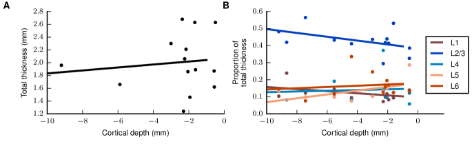
Figure S6: Related to Figure 1. Thickness versus cortical depth. (A) Total thickness vs. cortical depth and linear least-squares fit showing no significant correlation ($r=0.12,\>p=0.68$). (B) Relative laminar thicknesses vs. cortical depth and linear least-squares fits also showing no significant correlation (L1: $r=-0.43,\,p=0.14$, L2/3: $r=-0.46,\,p=0.11$, L4: $r=0.08,\>p=0.79$; L5: $r=-0.53,\>p=0.09$, L6: $r=0.14,\,p=0.69$). The thickness data is the same as in Figure 1. Cortical depth data obtained from F99 surface statistics available through the Caret Software (Van Essen, 2012). Values for each area are averaged across cortical surface and both hemispheres. The data is obtained using the F99 Sulcal depth tool on http://cocomac.g-node.org and can be directly accessed via these two links: http://cocomac.g-node.org/cocomac2/services/f99_sulcal_depth.php?atlas=FV91&shape=Depth-Right&mode=avg&output=tsv&run=1 and http://cocomac.g-node.org/cocomac2/services/f99_sulcal_depth.php?atlas=FV91&shape=Depth-Left&mode=avg&output=tsv&run=1.

We find total cortical thickness to decrease with logarithmized total neuron density. Similarly, total thicknesses from MR measurements decrease with architectural type (Wagstyl et al., 2015), which is known to correlate strongly with cell density (Hilgetag et al., 2015). In our data set, total and layer 4 thickness are also negatively correlated with architectural type, but these trends are less significant than those with logarithmized neuron density. Laminar and total cortical thicknesses are determined from micrographs, which has the drawback that this covers only a small fraction of the surface of each cortical area. For absolute but not relative thicknesses, another caveat is potential shrinkage and obliqueness of sections. It has also been found that relative laminar thicknesses depend on the sulcal or gyral location of areas, which is not offset by a change in neuron densities (Hilgetag & Barbas, 2006). However, regressing our relative thickness data against cortical depth of the areas registered to F99 revealed no significant trends of this type (Figure S6). Laminar thickness data are surprisingly incomplete, considering that this is a basic anatomical feature of cortex. In future, more systematic estimates from anatomical studies or MRI may become available. Total thicknesses have already recently been measured across cortex (Calabrese et al., 2015a; Wagstyl et al., 2015), and could complement the dataset used here covering 14 of the 32 areas. However, when computing numbers of neurons, using histological data may be preferable, because shrinkage effects on neuronal densities and laminar thicknesses partially cancel out.

In the model, we statistically assign synapses to target neurons based on anatomical reconstructions (Binzegger et al., 2004). On the target side, this yields similar laminar cell-body distributions for feedforward and feedback projections despite distinct laminar synapse distributions, mirroring findings in early visual cortex of mouse (De Pasquale & Sherman, 2011). Prominent experimental results on directional differences in communication patterns are based on LFP, ECoG and MEG recordings (van Kerkoerle et al., 2014; Bastos et al., 2015; Michalareas et al., 2016), which mostly reflect synaptic inputs. In future, these findings may be integrated into the stabilization procedure to better capture such differential interactions. While this is expected to enhance the distinction between average connection patterns for feedforward and feedback projections, known anatomical patterns suggest that a substantial fraction of individual pairs of areas deviate from a simple rule (Felleman & Van Essen, 1991; Krumnack et al., 2010; Bakker et al., 2012). The cortico-cortical connectivity may be further refined by incorporating the dual counterstream organization of feedforward and feedback connections (Markov et al., 2014b), or by taking into account different numbers of inter-area synapses per neuron in feedforward and feedback directions (Rockland, 2004).

In the resulting connectivity, we find multiple clusters reflecting the anatomical and functional partition of visual cortex into early visual areas, ventral and dorsal streams, parahippocampal and frontal areas, showing that the model construction yields a meaningful network structure. Moreover, the graded structural connectivity of the model agrees better with the experimentally measured resting-state activity than the binary connectivity from CoCoMac.

The network exhibits an asynchronous, irregular ground state across the network with population bursts due to inter-area interactions. Population firing rates differ across layers and inhibitory rates are generally higher than excitatory ones, in line with experimental findings (Swadlow, 1988; Fujisawa et al., 2008; Sakata & Harris, 2009). This can be attributed to the connectivity, because excitatory and inhibitory neurons are equally parametrized and excitatory neurons receive equal or stronger external stimulation compared to inhibitory ones. Laminar activity patterns vary across areas due to their customized structure and cortico-cortical connectivity.

Intrinsic single-cell time scales in the model are short in early visual areas and long in higher areas, on the same order of magnitude as found experimentally (Murray et al., 2014). The long time scales in higher areas are related to bursty firing associated with the high indegrees in these areas, but only occur in the presence of cortico-cortical interactions. Thus, the model predicts that the pattern of intrinsic time scales has a multi-scale origin. Systematic differences in synaptic composition across cortical regions and layers (Zilles et al., 2004; Hawrylycz et al., 2012) may also contribute to the experimentally observed pattern of time scales.

Inter-area interactions in the model are mainly mediated by population bursts of different lengths. The degree of synchrony accompanying inter-area interactions in the brain is as yet unclear. Obtaining substantial cortico-cortical interactions with low synchrony may be possible with finely structured connectivity and reduced noise input. When neurons are to a large extent driven by a noisy external input, a smaller percentage of their activity is determined by intrinsic inputs, which can decrease their effective coupling (Aertsen & Preißl, 1990). One way of reducing the external drive while preserving the mean network activity may be for the drive to be attuned to the intrinsic connectivity (Marre et al., 2009). Stronger intrinsic coupling while maintaining stability may be achieved for instance by introducing specific network structures such as synfire chains (Diesmann et al., 1999) or other feedforward structures, subnetworks, or small-world connectivity (Jahnke et al., 2014); population-specific patterns of short-term plasticity (Sussillo et al., 2007); or fine-tuned inhibition between neuronal groups (Hennequin et al., 2014).

The synchronous population events propagate stably across multiple areas, predominantly in the feedback direction. The systematic activation of parietal before occipital areas in the model is reminiscent of EEG findings on information flow during visual imagery (Dentico et al., 2014) and the top-down propagation of slow waves during sleep (Massimini et al., 2004; Nir et al., 2011; Sheroziya & Timofeev, 2014). Our method for determining the order of activations is similar to one recently applied to fMRI recordings (Mitra et al., 2014). It could be extended to distinguish between excitatory and inhibitory interactions like those we observe between V1 and frontal areas (Figure S4). In the network, cortico-cortical projections target both excitatory and inhibitory populations, with the majority of synapses terminating on excitatory cells. Stronger cortico-cortical synapses to enhance inter-area interactions require increased balancing of cortico-cortical inputs to preserve network stability. This is similar to the “handshake” mechanism in the microcircuit model of Potjans & Diesmann (2014) where interlaminar projections provide network stability by their inhibitory net effect.

The pattern of simulated interactions between areas resembles fMRI resting-state activity. The agreement between simulation and experiment peaks at intermediate coupling strength, where synchronized clusters also emerged most clearly in earlier models (Zhou et al., 2006; Deco & Jirsa, 2012). Furthermore, optimal agreement occurs just below a transition to a state where the network switches between attractors, supporting evidence that the brain operates in a slightly subcritical regime (Deco & Jirsa, 2012; Priesemann et al., 2014).

Time series of spiking activity reveal broad-band transmission between areas on time scales up to several seconds. The low-frequency part of these interactions is comparable to fMRI data, which describes coherent fluctuations on the order of seconds. The long time scales in the model activity may be caused by eigenmodes of the effective connectivity that are close to instability (Bos et al., 2015) or non-orthogonal (Hennequin et al., 2012). A potential future avenue for research would be to distinguish between such network effects and other sources of long time scales such as NMDA and $\mathrm{GABA_{B}}$ transmission, neuromodulation, or adaptation effects.

For tractability, the model represents each area as a $1\>\mathrm{mm}^{2}$ patch of cortex. True area sizes vary from $\sim\!3$ million cells in TH to $\sim\!300$ million cells in V1 for a total of around $8\cdot 10^{8}$ neurons in one hemisphere of macaque visual cortex, a model size that with recent advances in simulation technology (Kunkel et al., 2014) already fits on the most powerful supercomputers available today. Approaching this size would reduce the negative effects of downscaling (van Albada et al., 2015).

Overall, our model elucidates multi-scale relationships between cortical structure and dynamics, and can serve as a platform for the integration of new experimental data, the creation of hypotheses, and the development of functional models of cortex.

Experimental procedures

A: Model summary
Populations	254 populations: 32 areas (Table S1) with eight populations each (area TH: six)
Topology	—
Connectivity	area- and population-specific but otherwise random
Neuron model	leaky integrate-and-fire (LIF), fixed absolute refractory period (voltage clamp)
Synapse model	exponential postsynaptic currents
Plasticity	—
Input	independent homogeneous Poisson spike trains
Measurements	spiking activity

B: Populations
Type	Elements	Number of populations	Population size
Cortex	LIF neurons	32 areas with eight populations each (area TH: six), two per layer	$N$ (area- and population-specific)

C: Connectivity
Type	source and target neurons drawn randomly with replacement (allowing autapses and multapses) with area- and population-specific connection probabilities
Weights	fixed, drawn from normal distribution with mean $J$ and standard deviation $\delta J=0.1J$; 4E to 2/3E increased by factor $2$ (cf. Potjans & Diesmann, 2014); weights of inhibitory connections increased by factor $g$; excitatory weights $<0$ and inhibitory weights $>0$ are redrawn; cortico-cortical weights onto excitatory and inhibitory populations increased by factor $\lambda$ and $\lambda_{\mathcal{I}}\lambda$, respectively
Delays	fixed, drawn from Gaussian distribution with mean $d$ and standard deviation $\delta d=0.5d$; delays of inhibitory connections factor $2$ smaller; delays rounded to the nearest multiple of the simulation step size $h=0.1\,\mathrm{ms}$, inter-areal delays drawn from a Gaussian distribution with mean $d=s/v_{\mathrm{t}}$, with distance $s$ and transmission speed $v_{\mathrm{t}}=3.5\,\mathrm{m/s}$ (Girard et al., 2001); and standard deviation $\delta d=d/2$, distances determined as described in Supplemental Experimental Procedures, delays $<0.1\,\mathrm{ms}$ before rounding are redrawn

D: Neuron and synapse model
Name	LIF neuron
Type	leaky integrate-and-fire, exponential synaptic current inputs
Subthreshold dynamics	$\frac{\mathrm{d}V}{\mathrm{d}t}=-\frac{V-E_{\mathrm{L}}}{\tau_{\mathrm{m}}}+\frac{I_{\mathrm{s}}(t)}{C_{\mathrm{m}}}$  if $\mathrm{\left(t>t^{*}+\tau_{\text{r}}\right)}$ $V(t)=V_{\mathrm{r}}$          else $I_{\mathrm{s}}(t)=\sum_{i,k}J_{k}\,e^{-(t-t_{i}^{k})/\tau_{\mathrm{s}}}\Theta(t-t_{i}^{k})$ $k$: neuron index, $i$: spike index
Spiking	If $V(t-)<\theta\wedge V(t+)\geq\theta$ 1. set $t^{*}=t$, 2. emit spike with time stamp $t^{*}$

E: Input
Type	Target	Description
Background	LIF neurons	independent Poisson spikes (see Table S3)

F: Measurements

Spiking activity

Table 1: Model description after Nordlie et al. (2009).

In the following, we detail how we derive the structure of the model (summarized in Table 1), i.e., the population sizes, the local and cortico-cortical connectivity and the external drive.

Numbers of neurons

We estimate the number of neurons $N(A,i)$ in population $i$ of area $A$ in three steps:

1. We translate neuronal volume densities to the FV91 scheme from the most representative area in the original scheme (Table S4). For areas not covered by the data set, we take the average laminar densities for areas of the same architectural type. Table 4 of Hilgetag et al. (2015) lists the architectural types, which we translate to the FV91 scheme according to Table S4. To the previously unclassified areas MIP and MDP we manually assign type 5 like their neighboring area PO, which is similarly involved in visual reaching (Johnson et al., 1996; Galletti et al., 2003), and was placed at the same hierarchical level by Felleman & Van Essen (1991).

2. We determine total and laminar thicknesses as detailed in Results.

3. The fraction $\gamma(v)$ of excitatory neurons in layer $v$ is taken to be identical across areas. For the laminar dependency, values from cat V1 (Binzegger et al., 2004) are used with 78% excitatory neurons in layer 2/3, 80% in L4, 82% in L5, and 83% in L6.

The resulting number of neurons in population $i$ of area $A$ is

$$N(A,i)=\rho\left(A,v{}_{i}\right)S(A)D\left(A,v{}_{i}\right)\cdot\negthickspace\negthickspace\negthickspace \begin{cases}\gamma\left(v{}_{i}\right)&\textrm{if }i\in\mathcal{E}\\ 1-\gamma\left(v{}_{i}\right)&\textrm{\text{if }}i\in\mathcal{I}\end{cases}$$ , (1)

where $v_{i}$ denotes the layer of population $i$, $S(A)$ the surface area of area $A$ (cf. Table S7), $D(A,v{}_{i})$ the thickness of layer $v{}_{i}$, and $\mathcal{E},\mathcal{\,I}$ the pool of excitatory and inhibitory populations, respectively. Table S8 gives the population sizes corresponding to the modeled $1\>\mathrm{mm}^{2}$ area size.

Local connectivity

The connection probabilities of the microcircuit model (Potjans & Diesmann, 2014, Table 5), computed from anatomical and electrophysiological studies (with large contributions from Binzegger et al., 2004; Thomson & Lamy, 2007), form the basis for the local circuit of each area. The connectivity between any pair of populations is spatially uniform. However, we take the underlying probability $C$ for a given neuron pair to establish one or more contacts to decay with distance according to a Gaussian with standard deviation $\sigma=297\,\mathrm{\mu m}$ (Potjans & Diesmann, 2014). We approximate each brain area as a flat disk with (area-specific) radius $R$ and assign polar coordinates $r$ and $\theta$ to each neuron. The radius determines the cut-off of the Gaussian and hence the precise connectivities. The average connection probability is obtained by integrating over all possible positions of the two neurons:

$$\bar{C}(R)=\frac{C_{0}}{\pi^{2}R^{4}}\int_{0}^{R}\int_{0}^{2\pi}\int_{0}^{R}\int_{0}^{2\pi}\exp\left[\frac{-\left(r_{1}^{2}+r_{2}^{2}-2r_{1}r_{2}\cos(\theta_{1}-\theta_{2})\right)}{2\sigma^{2}}\right]r_{1}r_{2}\mathrm{d}\theta_{1}\mathrm{d}r_{1}\mathrm{d}\theta_{2}\mathrm{d}r_{2}\,,$$ (2)

with $C_{0}$ the connection probability at zero distance. This can be reduced to a simpler form (Sheng, 1985),

$$\bar{C}(R)=\frac{2C_{0}}{\pi R^{2}}\int_{0}^{2R}e^{-r^{2}/2\sigma^{2}}\left[4\arctan\left(\frac{2R-r}{2R+r}\right)^{1/2}-\sin\left(4\arctan\left[\frac{2R-r}{2R+r}\right]^{1/2}\right)\right]r\mathrm{d}r\,.$$ (3)

Averaged across population pairs, $C_{0}$ is $0.143$ (computed from Eq. 8 and Table S1 in Potjans & Diesmann, 2014). Note that Potjans & Diesmann (2014) only vary the position of one neuron, keeping the other neuron fixed in the center of the disk (Eq. 9 in that paper). Henceforth, we denote connection probabilities computed with the latter approach with the subscript $\mathrm{PD14}$ and use primes for all variables referring to a network with the population sizes of the microcircuit model.

The parameters of the microcircuit model are reported for a $1\>\mathrm{mm}^{2}$ patch of cortex, corresponding to $R=\sqrt{1/\pi}\,\mathrm{mm}$, which we call $R_{0}$. For each source population $j$ and target population $i$, we first translate the connection probabilities of the $1\>\mathrm{mm}^{2}$ model to area-dependent $R$ via

$$C_{ij}^{\prime}(R)=C_{ij,\mathrm{PD14}}^{\mathrm{\prime}}\left(R_{0}\right)\frac{\bar{C}^{\prime}(R)}{\bar{C}_{\mathrm{PD14}}^{\prime}\left(R_{0}\right)}\,,$$

with $\bar{C}_{\mathrm{PD14}}^{\prime}(R_{0})=0.066$. From this, we compute the number of synapses

$$N_{\mathrm{syn},ij}=\frac{\log\left(1-C_{ij}\right)}{\log\left(1-\frac{1}{N_{i}N_{j}}\right)}\,,$$

based on randomly drawing source and target neurons with replacement (cf. Eq. 1 in Potjans & Diesmann, 2014). The indegree $K_{ij}$ is the number of incoming synapses per target neuron, $N_{\mathrm{syn},ij}/N_{i}$. Henceforth, all numbers of synapses $N_{\mathrm{syn}}(A)$ and indegrees $K_{ij}(A)$ are area-specific. For simplicity, we drop the argument $A$. Since mean synaptic inputs are proportional to the indegrees, we consider them a defining characteristic of the local circuit and preserve their relative values when adjusting the model to area-specific population sizes,

$$\frac{K_{ij}(R)}{K_{kl}(R)}=\frac{K_{ij}^{\prime}(R)}{K_{kl}^{\prime}(R)}\,\,\,\forall i,j,k,l$$

$$\Leftrightarrow K_{ij}(R)=c_{A}(R)K_{ij}^{\mathrm{\prime}}(R)\,\,\,\forall i,j\,,$$ (4)

with $c_{A}(R)$ an area-specific conversion factor, which is larger for areas with smaller neuron densities because of the assumption of constant synaptic volume density. It is computed as

$$c_{A}(R)=\frac{N_{\mathrm{syn,tot}}(R)}{\sum_{i,j}N_{i}K_{ij}^{\prime}}\,\mathit{FLN}_{\mathrm{i}}\Bigg{\langle}\frac{K_{ij}^{\prime}(R)}{K_{ij}^{\prime}(R_{\mathrm{full}})}\Bigg{\rangle}_{ij}\,,$$

with $FLN_{\mathrm{i}}$ the fraction of labeled neurons intrinsic to the injected area in a retrograde tracing experiment by Markov et al. (2011) and $N_{\mathrm{syn,tot}}(R)=\rho_{\mathrm{syn}}\pi R^{2}D$ with $D$ the total thickness of the given area. For details, see Supplemental Experimental Procedures.

Cortico-cortical connectivity

We determine whether a pair of areas is connected using the union of all connections reported in the FV91 scheme in the CoCoMac database (Stephan et al., 2001; Bakker et al., 2012; Suzuki & Amaral, 1994a; Felleman & Van Essen, 1991; Rockland & Pandya, 1979; Barnes & Pandya, 1992) (Figure 1F, see Supplemental Experimental Procedures for details) and all connections reported by Markov et al. (2014a). We then determine population-specific numbers of modeled cortico-cortical synapses in three steps: 1.  deriving the area-level connectivity; 2. distributing synapses across layers; 3. assigning synapses to target neurons.

For the first step, we compute the total number of synapses formed between each pair of areas using retrograde tracing data from Markov et al. (2014a). The data consist of fractions of labeled neurons $\mathit{FLN}_{AB}=NLN_{AB}/\sum_{B^{\prime}}NLN_{AB^{\prime}}$, with $NLN_{AB}$ the number of labeled neurons in area $B$ upon injection in area $A$. Markov et al. (2014a) used a parcellation scheme called M132 which is also available as a cortical surface, both in native and in F99 space. On the target side we use the coordinates of the injection sites registered to the F99 atlas available via the Scalable Brain Atlas (Bakker et al., 2015) to identify the equivalent area in the FV91 parcellation (cf. Table S9). There is data for 11 visual areas in the FV91 scheme with repeat injections in six areas, for which we take the arithmetic mean. To map data on the source side from M132 to FV91, we count the number of overlapping triangles on the F99 surface between any given pair of regions and distribute the $FLN$ proportionally to the amount of overlap, using the F99 region overlap tool at the CoCoMac site (http://cocomac.g-node.org). To estimate values for the areas not included in the data set, we use an exponential decay of connectivities with distance (Ercsey-Ravasz et al., 2013),

$$FLN_{AB}=C\cdot\exp\left(-\lambda d_{AB}\right)\,.$$ (5)

A linear least-squares fit of the logarithm of the $FLN$ (Figure 1G) predicts missing values. The total number of synapses $N_{\mathrm{syn},AB}$ between each pair of areas $\{A,B\}$ is assumed to be proportional to the number of labeled neurons $NLN_{AB}$ and thus to $FLN_{AB}$,

$$\frac{N_{\mathrm{syn},AB}}{\underbrace{\sum_{B^{\prime}}N_{\mathrm{syn,}AB^{\prime}}}_{=N_{\mathrm{syn,tot},A}}}=\frac{NLN_{AB}}{\sum_{B^{\prime}}NLN_{AB^{\prime}}}=\frac{FLN_{AB}}{\sum_{B^{\prime}}FLN_{AB^{\prime}}}.$$

This corresponds to individual neurons in each source area (including area $A$ itself) on average establishing the same number of synapses in the target area $A$. For each target area, the $FLN$ in the model should add up to the total fraction of connections from visual cortical areas, which is not known a priori. For normalization, we consider also non-visual areas, for which distances are available and for which we can hence also estimate the $FLN$. The total fraction of all connections from subcortical regions averages $1.3\,\%$ in eight cortical areas (Markov et al., 2011). This allows us to normalize the combined $FLN$ from all cortical areas as $\sum_{B}FLN_{AB}=1-FLN_{\mathrm{i}}-0.013$, where the sum includes both modeled and non-modeled cortical areas.

As a next step, we determine the distribution of connections across source and target layers. On the source side, the laminar projection pattern can be expressed as the fraction of supragranular labeled neurons ($\mathit{SLN}$) in retrograde tracing experiments (Markov et al., 2014b). To determine the $SLN$ entering into the model, we use the exact coordinates of the injections to determine the corresponding target area $A$ in the FV91 parcellation, and for each pair of areas we take the mean $SLN$ across injections. To map the data from M132 to FV91, we weight the $SLN$ by the overlap $c_{B,\beta}$ between area $\beta$ in the former and area $B$ in the latter scheme and the $FLN$ to take into account the overall strength of the connection,

$$SLN_{AB}=\frac{\sum_{\beta}c_{B,\beta}FLN_{A,\beta}SLN_{A,\beta}}{\sum_{\beta}c_{B,\beta}FLN_{A,\beta}}\,.$$

We estimate missing values using a sigmoidal fit of $SLN$ vs. the logarithmized ratio of overall cell densities of the two areas (Figure 1J). A relationship between laminar patterns and log ratios of neuron densities was suggested by Beul et al. (2015). Following Markov et al. (2014b), we use a generalized linear model and assume the numbers of labeled neurons in the source areas to sample from a beta-binomial distribution (e.g. Weisstein, 2005). This distribution arises as a combination of a binomial distribution with probability $p$ of supragranular labeling in a given area, and a beta distribution of $p$ across areas with dispersion parameter $\phi$. With the probit link function $g$ (e.g. McCulloch et al., 2008), the measured $SLN$ relates to the log ratio $\ell$ of neuron densities for each pair of areas as

$$g(SLN)=a_{0}\left(\begin{array}[]{c}1\\ \vdots\\ 1\end{array}\right)+a_{1}\ell,$$ (6)

where $\ell$ and $SLN$ are vectors and $\{a_{0},a_{1}\}$ are scalar fit parameters. To fit $SLN$ vs. log ratios of cell densities, we map the FV91 areas to the Markov et al. (2014b) scheme with the overlap tool of CoCoMac (see above) and compute the cell density of each area in the M132 scheme as a weighted average over the relevant FV91 areas. For areas with identical names in both schemes, we simply take the neuron density from the FV91 scheme. Figure 1J shows the result of the $SLN$ fit in R (R Core Team, 2015) with the betabin function of the aod package (Lesnoff & Lancelot, 2012). In contrast to Markov et al. (2014b), who exclude certain areas when fitting $SLN$ vs. hierarchical distances in view of ambiguous hierarchical relations, we take all data points into account to obtain a simple and uniform rule.

As a further step, we combine $SLN$ with CoCoMac data. The data sets complement each other: $SLN$ provides quantitative data on laminar patterns of incoming projections for about one quarter of the connected areas. CoCoMac has values for all six layers, but limited to a qualitative strength ranging from 0 (absent) to 3 (strong) which we take to represent numbers of synapses in orders of magnitude (see Supplemental Experimental Procedures). Whether or not to include a layer in source pattern $P_{\mathrm{s}}$ is based on CoCoMac (Felleman & Van Essen, 1991; Barnes & Pandya, 1992; Suzuki & Amaral, 1994b; Morel & Bullier, 1990; Perkel et al., 1986; Seltzer & Pandya, 1994) if the corresponding data is available ($45\,\%$ coverage); otherwise, we include L2/3, L5 and L6 and exclude L4 (Felleman & Van Essen, 1991). We model cortico-cortical connections as purely excitatory, a good approximation to experimental findings (Salin & Bullier, 1995; Tomioka & Rockland, 2007). If a layer is included in the source pattern, we assign a fraction of the total outgoing synapses to it according to the $SLN$. Since the $SLN$ do not further distinguish between the infragranular layers 5 and 6, we use the rough connection densities from CoCoMac for this purpose when available, and otherwise we distribute synapses in proportion to the numbers of neurons. On the target side, we determine the pattern of target layers $P_{\mathrm{t}}$ from anterograde tracer studies in CoCoMac (Jones et al., 1978; Rockland & Pandya, 1979; Morel & Bullier, 1990; Webster et al., 1991; Felleman & Van Essen, 1991; Barnes & Pandya, 1992; Distler et al., 1993; Suzuki & Amaral, 1994b; Webster et al., 1994) if available (29% coverage); otherwise we use termination patterns suggested by the $SLN$ based on a relationship between source and target patterns. Using the terminology of visual connection hierarchies, we denote projections with low, intermediate, and high $SLN$ respectively as feedback, lateral, and feedforward projections. We take $SLN<0.35$ to correspond to feedback projections, $SLN>0.65$ to feedforward projections and $SLN\in[0.35,0.65]$ to lateral projections. The corresponding termination patterns $P_{\mathrm{t}}$ are

$$\begin{split}\{4\}\,\text{for }SLN>0.65\\ \{1,2/3,5,6\}\,\text{for }SLN<0.35\\ \{1,2/3,4,5,6\}\,\text{for }SLN\in[0.35,0.65]\end{split}\,,$$

and we distribute synapses among the layers in the termination pattern in proportion to their thickness.

Since we use a point neuron model, we have to account for the possibly different laminar positions of cell bodies and synapses. The data of Binzegger et al. (2004) deliver three quantities that allow us to relate synapse to cell body locations: first, the probability $\mathcal{P}(s_{\mathrm{cc}}|c_{\mathrm{B}}\bigcap s\in v)$ for a synapse in layer $v$ on a cell of type $c_{\mathrm{B}}$ (e.g., a pyramidal cell with soma in L5) to be of cortico-cortical origin; second, the relative occurrence $\mathcal{\mathcal{\mathcal{P}}}(c_{\mathrm{B}})$ of the cell type $c_{\mathrm{B}}$; and third, the total numbers of synapses $N_{\mathrm{syn}}(v,c_{\mathrm{B}})$ in layer $v$ onto the given cell type. We map these data to our model by computing the conditional probability $\mathcal{P}(i|s_{\mathrm{cc}}\in v)$ for the target neuron to belong to population $i$ if a cortico-cortical synapse $s_{\mathrm{cc}}$ is in layer $v$. This probability equals the sum of probabilities that a synapse is established on the different Binzegger et al. subpopulations making up our populations,

$$\mathcal{P}(i|s_{\mathrm{cc}}\in v)=\mathcal{P}(\bigcup_{\mathrm{c_{\mathrm{B}}}\in i}c_{\mathrm{B}}|s_{\mathrm{cc}}\in v)=\sum_{c_{\mathrm{B}}\in i}\mathcal{P}(c_{\mathrm{B}}|s_{\mathrm{cc}}\in v)\,,$$ (7)

where

$$\mathcal{P}(c_{\mathrm{B}}|s_{\mathrm{cc}}\in v)=\frac{\mathcal{P}(c_{\mathrm{B}}\bigcap s_{\mathrm{cc}}\in v)}{\mathcal{P}(s_{\mathrm{cc}}\in v)}\,.$$ (8)

The numerator gives the joint probability that a cortico-cortical synapse is formed in layer $v$ on cell type $c_{\mathrm{B}}$,

$$\mathcal{P}(c_{\mathrm{B}}\bigcap s_{\mathrm{cc}}\in v)=\frac{N_{\mathrm{syn,CC}}(v,c_{\mathrm{B}})\mathcal{P}(c_{\mathrm{B}})}{\sum_{v^{\prime},c_{\mathrm{B}}^{\prime}}N_{\mathrm{syn,CC}}(v{}^{\prime},c_{\mathrm{B}}^{\prime})\mathcal{P}(c_{\mathrm{B}}^{\prime})}\,,$$

and the denominator is the probability of a cortico-cortical synapse in layer $v$, computed by summing over cell types,

$$\mathcal{P}(s_{\mathrm{cc}}\in v)=\sum_{c_{\mathrm{B}}}\mathcal{P}(c_{\mathrm{B}}\bigcap s_{\mathrm{cc}}\in v)\,.$$

$N_{\mathrm{syn,CC}}(v,c_{\mathrm{B}})$ represents the number of cortico-cortical synapses in layer $v$ on cell type $c_{\mathrm{B}}$,

$$N_{\mathrm{syn,CC}}(v,c_{\mathrm{B}})=\mathcal{P}(s_{\mathrm{cc}}|c_{\mathrm{B}}\bigcap s\in v)\,N_{\mathrm{syn}}(v,c_{\mathrm{B}})\,\mathcal{\mathcal{\mathcal{P}}}(c_{\mathrm{B}})\,,$$

which can be directly determined from the data. Combining these equations, we obtain the number of cortico-cortical (type III) synapses from excitatory population $j$ of area $B$ to population $i$ of area $A$ (cf. Figure 1K):

$$N_{\mathrm{syn},\mathrm{III}}(i,A,j,B) = \underbrace{Z_{i}\sum_{v\in P_{\mathrm{t}}}Y_{v}\,\mathcal{P}(i|s_{\mathrm{cc}}\in v)}_{\text{target side}}\,\underbrace{X_{j}}_{\text{source side}}N_{\mathrm{syn},\mathrm{III}}(A,B)\,,$$ (9)

$$\text{with \,}X_{j} = \begin{cases}\mathit{SLN}&\textrm{if }j\in S\bigcap P_{\text{s}}\\ (1-\mathit{SLN})\frac{10^{\alpha(v_{j})}}{\sum_{j^{\prime}\in I,\,\alpha(v_{j^{\prime}})>0}10^{\alpha(v_{j^{\prime}})}}&\text{if }j\in I\,\text{and }\alpha(v_{j})>0\\ (1-\mathit{SLN})\frac{N(A,j)}{{}_{\sum_{j^{\prime}\in I}N(A,j^{\prime})}}&\textrm{\text{if }}j\in I\bigcap P_{\text{s}}\text{\, but no CoCoMac data available}\\ 0&\text{if }j\notin P_{\mathrm{s}}\end{cases}\,,$$

$$\text{and \,}Y_{v} = \begin{cases}\frac{10^{\alpha(v)}}{\sum_{\alpha(v^{\prime})>0}10^{\alpha(v^{\prime})}}&\text{if\,}\alpha(v)>0\\ \frac{D(A,v)}{\sum_{v^{\prime}}D(A,v^{\prime})}&\text{if no CoCoMac data available\,}\end{cases}\,.$$

Here, $S=\text{2/3E}$ and $I=\left\{\text{5E,6E}\right\}$ respectively denote the supragranular and infragranular excitatory populations. $Z_{i}$ is an additional factor which takes into account that cortico-cortical feedback connections preferentially target excitatory rather than inhibitory neurons (Johnson & Burkhalter, 1996; Anderson et al., 2011). $Z_{i}$ is area-specific and depends on the excitatory or inhibitory nature of the target population, but not on the target layer. We choose a fraction of $93\,\%$ of connections targeting excitatory neurons, as an average over experimental values ranging between $87\,\%$ and $98\,\%$. For each feedback connection in the model, we thus redistribute the synapses across the excitatory and inhibitory target populations and determine $Z_{i}$ such that

$$\frac{\sum_{i\in\mathcal{E}}\sum_{j}N_{\mathrm{syn},\mathrm{III}}(i,A,j,B)}{N_{\mathrm{syn},\mathrm{III}}(A,B)}=0.93\,.$$

Figure S1 shows the resulting connection probabilities between all population pairs in the model.

External, random input

Since quantitative area-specific data on non-visual and subcortical inputs are highly incomplete, we use a simple scheme to determine numbers of external inputs: For each area, we compute the total number of external synapses as the difference between the total number of synapses and those of type I and III and distribute these such that all neurons in the given area have the same indegree for Poisson sources. In area TH, we compensate for the missing granular layer 4 by increasing the external drive onto populations 2/3E and 5E by $20\,\%$. With the modified connectivity matrix yielded by the analytical procedure described in Schuecker et al. (2015), we set $\kappa=1.125$ to increase the external indegree onto population 5E by $12.5\,\%$ and onto 6E by $42\,\%$ to elevate the firing rates in these populations. Table S11 lists the resulting external indegrees.

Network simulations

We performed simulations on the JUQUEEN supercomputer (Jülich Supercomputing Centre, 2015) with NEST version 2.8.0 (Eppler et al., 2015) with optimizations for the use on the supercomputer which will be included in a future release. All simulations use a time step of $0.1\>\mathrm{ms}$ and exact integration for the subthreshold dynamics of the LIF neuron model (reviewed in Plesser & Diesmann, 2009). Simulations were run for $100.5\>\mathrm{s}$ ($\lambda=1.9$), $50.5\>\mathrm{s}$ ($\lambda\in[1.8,\,2.0,\,2.1]$), and $10.5\>\mathrm{ms}$ ($\lambda\in[1.,\,1.5,\,1.7,\,2.5]$) biological time discarding the first $500\>\mathrm{ms}$. Spike times were recorded from all neurons, except for the simulations shown in Figure 2A,B, where we recorded from 1000 neurons per population.

Analysis methods

We investigate the structural properties of the model with the map equation method (Rosvall et al., 2010). In this clustering algorithm, an agent performs random walks between graph nodes with probability proportional to the outdegree of the present node and a probability ($p=0.15$) of jumping to a random network node. The algorithm detects clusters in the graph by minimizing the length of a binary description of the network using a Huffman code. To assess the quality of the clustering, we use a modularity measure which extends a measure for unweighted, directed networks (Leicht & Newman, 2008) to weighted networks, analogous to Newman 2004,

$$Q=\frac{1}{m}\sum_{A,B}\left(\mathcal{O}_{AB}-\frac{\sum_{B^{\prime}}\mathcal{O}_{AB^{\prime}}\cdot\sum_{A^{\prime}}K_{A^{\prime}B}}{m}\right)\delta_{\mathcal{C}_{A},\mathcal{C}_{B}}\,,$$

where $\mathcal{O}_{AB}$($K_{AB}$) is the matrix of relative outdegrees (indegrees), $m=\sum_{A,B}\mathcal{O}_{A,B}$ and $\delta_{\mathcal{C}_{A},\mathcal{C}_{B}}=1$ if areas $A$ and $B$ are in the same cluster and 0 otherwise. $Q=0$ reflects equal connectivity within and between clusters, while $Q=1$ corresponds to connectivity exclusively within clusters.

Instantaneous firing rates are determined as spike histograms with bin width $1\>\mathrm{ms}$ averaged over the entire population or area. In Figure 4G, Figure S2G, and to determine the temporal hierarchy, we convolve the histograms with Gaussian kernels with $\sigma=2\>\mathrm{ms}$. Spike-train irregularity is quantified for each population by the revised local variation $LvR$ (Shinomoto et al., 2009) averaged over a subsample of $2000$ neurons. The cross-correlation coefficient is computed with bin width $1\>\mathrm{ms}$ on single-cell spike histograms of a subsample of $2000$ neurons per population with at least one emitted spike per neuron.

The single-cell autocorrelation function is calculated on spike histograms with bin width $2.5\>\mathrm{ms}$ to suppress fast fluctuations on the order of the refractory time, normalized to the zero-lag peak, and averaged across a subsample of $2000$ neurons. We then perform a linear least-squares fit $f(t)=A-t/\tau$ on the logarithmized autocorrelation for all times $t\in\left[2.5,\,75\right]$ and define the inverse slope $\tau$ as the intrinsic time scale of the population. If the autocorrelation drops to a local minimum at the first time lag $t=2.5\>\mathrm{ms}$, we set the time scale to the refractory period, $\tau=2\>\mathrm{ms}$.

The temporal hierarchy is based on the cross-covariance function between area-averaged firing rates. We use a wavelet-smoothing algorithm (signal.find_peaks_cwt of python scipy library (Jones et al., 2001) with peak width $\Delta=20\>\mathrm{ms}$) to detect extrema for $\tau\in[-100,\,100]$ and take the location of the extremum with the largest absolute value as the time lag.

Functional connectivity (FC) is defined as the zero-time lag cross-correlation coefficient of the area-averaged synaptic inputs

$$I_{A}(t)=\frac{1}{N_{A}}\sum_{i\in A}N_{i}\left|I_{i}(t)\right|=\frac{1}{N_{A}}\sum_{i\in A}N_{i}\sum_{j}K_{ij}\left|J_{ij}\right|\left(\nu_{j}\ast PSC_{j}\right)(t)\>,$$

with the normalized post-synaptic current $PSC_{j}(t)=\exp[-t/\tau_{\mathrm{s}}]$, the population firing rate $\nu_{j}$ of source population $j$, indegree $K_{ij}$, and synaptic weight $J_{ij}$ of the connection from $j$ to target population $i$ containing $N_{i}$ neurons.

The clustering of the FC matrices was performed using the function modularity_louvain_und_sign of the Brain Connectivity Toolbox (BCT; http://www.brain-connectivity-toolbox.net) with the $Q^{\ast}$ option, which weights positive weights more strongly than negative weights, as introduced by Rubinov & Sporns (2011).

Macaque resting-state fMRI

Data were acquired from six male macaque monkeys (4 Macaca mulatta and 2 Macaca fascicularis). All experimental protocols were approved by the Animal Use Subcomittee of the University of Western Ontario Council on Animal Care and in accordance with the guidelines of the Canadian Council on Animal Care. Data acquisition, image preprocessing and a subset of subjects (5 of 6) were previously described (Babapoor-Farrokhran et al., 2013). Briefly, 10 5-min resting-state fMRI scans (TR: $2\>\mathrm{s}$; voxel size: $1\>\mathrm{mm}$ isotropic) were acquired from each subject under light anaesthesia ($1.5$ isoflurane). Additional processing for the current study included the regression of nuisance variables using the AFNI software package (afni.nimh.nih.gov/afni), which included six motion parameters as well as the global white matter and CSF signals. The global mean signal was not regressed.

The FV91 parcellation was drawn on the F99 macaque standard cortical surface template (Van Essen et al., 2001) and transformed to volumetric space with a $2\>\mathrm{mm}$ extrusion using the Caret software package (http://www.nitrc.org/projects/caret). The parcellation was applied to the fMRI data and functional connectivity computed as the Pearson correlation coefficients between probabilistically-weighted ROI timeseries for each scan (Shen et al., 2012). Correlation coefficients were Fisher z-transformed and correlation matrices were averaged within animals and then across animals before transforming back to Pearson coefficients.

Author Contributions

Conceptualization: M.D., S.J.v.A., M.S.; Software: M.S., R.B., S.J.v.A.; Investigation: M.S., S.J.v.A.; Writing - Original Draft: M.S., S.J.v.A.; Writing - Review & Editing: M.S., S.J.v.A., R.B., C.-C.H., M.D.; Resources: R.B., K.S., G.B., C.-C.H.; Funding Acquisition: M.D., M.S., S.J.v.A., R.B.; Supervision: S.J.v.A., M.D.

Supplemental Figures

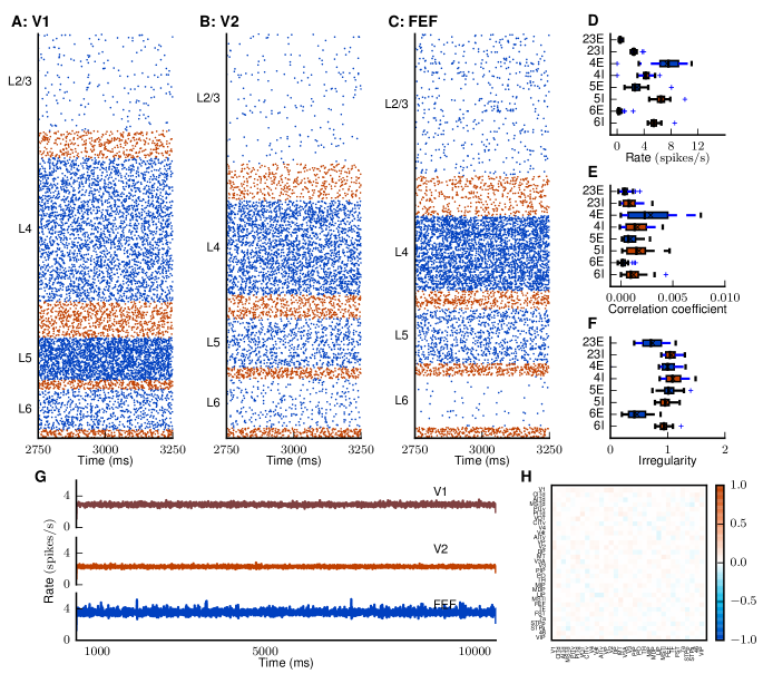
Figure S2: Related to Figure 4. Resting state of the model with cortico-cortical synaptic weights equal to intrinsic synaptic weights. (A-C) Raster plot of spiking activity of $5\,\%$ of the neurons in area V1 (A), V2 (B), and FEF (C). (D-F) Statistics of the spiking activity across areas and populations shown as area-averaged box plots (Tukey, 1977). (D) Population-averaged firing rates. The firing rates differ across areas and layers, varying between $0.05$ and $25\;\mathrm{spikes}/\mathrm{s}$. Inhibitory populations are more active than excitatory populations across layers and areas (with the exception of layer 5 in V1 and layer 4 in higher areas) despite the identical intrinsic properties of the two cell types. The excitatory populations of layer 2/3 and 6 exhibit lower firing rates than those of layers 4 and 5, similar to the microcircuit model (Potjans & Diesmann, 2014) (E) Average pairwise cross-correlation coefficients of spiking activity. (F) Irregularity measured by revised local variation $LvR$ (Shinomoto et al., 2009) averaged across neurons. (G) Area-averaged firing rates. Parameters are $g=-11,\>\nu_{\mathrm{ext}}=10\;\mathrm{spikes}/\mathrm{s},\>\kappa=1.125,\>\lambda=1,\>\lambda_{\mathcal{I}}=1$. (H) Functional connectivity (FC) in the model for measured by the zero-time lag cross-correlation coefficiens. Functional connectivity between areas is very low for most pairs of areas. Areas are ordered as in Figure 7A.

Supplemental Experimental Procedures

Cortical areas in the model

Lobe	Abbreviation	Brain Region
Occipital	V1	Visual area 1
	V2	Visual area 2
	V3	Visual area 3
	VP	Ventral posterior
	V3A	Visual area V3A
	V4	Visual area 4
	VOT	Ventral occipitotemporal
	V4t	V4 transitional
	MT	Middle temporal
Temporal	FST	Floor of superior temporal
	PITd	Posterior inferotemporal (dorsal)
	PITv	Posterior inferotemporal (ventral)
	CITd	Central inferotemporal (dorsal)
	CITv	Central inferotemporal (ventral)
	AITd	Anterior inferotemporal (dorsal)
	AITv	Anterior inferotemporal (ventral)
	STPp	Superior temporal polysensory (posterior)
	STPa	Superior temporal polysensory (anterior)
	TF	Parahippocampal area TF
	TH	Parahippocampal area TH
Parietal	MSTd	Medial superior temporal (dorsal)
	MSTl	Medial superior temporal (lateral)
	PO	Parieto-occipital
	PIP	Posterior intraparietal
	LIP	Lateral intraparietal
	VIP	Ventral intraparietal
	MIP	Medial intraparietal
	MDP	Medial dorsal parietal
	DP	Dorsal prelunate
	7a	7a
Frontal	FEF	Frontal eye field
	46	Middle frontal area 46

Table S1: List of areas in the model. All vision-related areas of macaque cortex in the parcellation of Felleman & Van Essen (1991).

Inter-areal distances

Area	V1	V2	VP	V3	V3A	MT	V4t	V4	VOT	MSTd	PIP	PO	DP	MIP	MDP	VIP
V1	0.0	17.9	19.9	14.6	16.8	22.5	23.1	22.9	29.0	26.8	18.8	21.5	23.7	24.5	29.2	26.3
V2	17.9	0.0	16.1	17.8	18.2	20.0	20.5	21.2	24.5	24.4	19.8	23.8	24.6	26.0	30.8	25.8
VP	19.9	16.1	0.0	20.8	19.0	14.9	15.1	14.6	12.8	20.9	20.1	25.2	25.4	26.9	31.9	25.5
V3	14.6	17.8	20.8	0.0	8.1	15.9	17.0	18.5	26.9	19.4	10.6	14.6	15.1	16.9	22.0	18.1
V3A	16.8	18.2	19.0	8.1	0.0	12.4	13.4	15.6	23.4	15.4	9.2	15.0	9.4	16.3	21.2	13.8
MT	22.5	20.0	14.9	15.9	12.4	0.0	6.0	11.4	13.7	10.0	13.2	19.1	16.6	20.0	23.9	13.7
V4t	23.1	20.5	15.1	17.0	13.4	6.0	0.0	9.9	12.1	12.1	15.2	21.3	17.8	22.1	26.3	16.4
V4	22.9	21.2	14.6	18.5	15.6	11.4	9.9	0.0	13.1	17.8	18.6	24.6	20.4	25.6	30.5	21.4
VOT	29.0	24.5	12.8	26.9	23.4	13.7	12.1	13.1	0.0	19.7	24.6	30.0	28.5	31.0	36.0	26.6
MSTd	26.8	24.4	20.9	19.4	15.4	10.0	12.1	17.8	19.7	0.0	14.5	20.6	17.1	20.2	24.1	11.5
PIP	18.8	19.8	20.1	10.6	9.2	13.2	15.2	18.6	24.6	14.5	0.0	9.5	12.3	9.8	14.2	11.2
PO	21.5	23.8	25.2	14.6	15.0	19.1	21.3	24.6	30.0	20.6	9.5	0.0	18.9	6.9	10.0	16.0
DP	23.7	24.6	25.4	15.1	9.4	16.6	17.8	20.4	28.5	17.1	12.3	18.9	0.0	18.3	22.0	11.1
MIP	24.5	26.0	26.9	16.9	16.3	20.0	22.1	25.6	31.0	20.2	9.8	6.9	18.3	0.0	6.3	14.6
MDP	29.2	30.8	31.9	22.0	21.2	23.9	26.3	30.5	36.0	24.1	14.2	10.0	22.0	6.3	0.0	17.4
VIP	26.3	25.8	25.5	18.1	13.8	13.7	16.4	21.4	26.6	11.5	11.2	16.0	11.1	14.6	17.4	0.0
LIP	27.8	27.6	28.0	19.3	14.6	16.0	18.6	23.3	29.1	12.4	13.6	19.5	10.1	18.2	21.1	7.4
PITv	32.9	28.0	16.8	30.4	26.8	16.3	14.8	16.3	7.4	21.5	27.6	32.9	31.9	34.0	38.7	28.8
PITd	31.6	27.3	17.8	27.4	23.5	13.1	11.6	14.1	8.6	18.7	24.8	30.6	28.2	31.4	35.9	25.7
MSTl	28.4	24.4	17.4	22.6	18.9	8.2	9.9	15.7	13.2	9.1	18.0	24.0	22.7	24.2	28.3	16.9
CITv	38.8	33.4	22.4	36.0	32.7	21.6	21.1	22.5	12.9	25.7	32.4	37.6	37.7	38.8	43.1	33.1
CITd	37.7	32.5	22.0	34.3	31.0	19.5	19.2	20.9	12.2	23.2	30.5	35.9	35.7	37.0	41.0	30.7
FEF	57.1	53.9	48.3	50.0	45.8	37.9	40.3	45.8	42.1	36.4	42.9	47.9	46.2	45.4	46.7	36.8
TF	29.6	24.8	16.3	27.4	24.7	15.8	17.1	20.1	14.4	20.2	23.5	28.0	29.8	29.5	33.7	25.9
AITv	43.8	38.2	28.2	41.1	38.1	26.6	27.0	28.9	19.5	30.1	36.7	41.4	42.7	42.5	46.7	36.5
FST	33.7	28.9	20.3	28.8	25.6	14.2	15.7	19.2	12.8	16.5	24.6	29.8	29.6	30.6	34.2	23.8
7a	28.2	27.6	27.4	19.9	14.5	15.5	18.0	22.4	27.8	11.0	14.5	20.9	11.5	20.0	23.2	9.4
STPp	38.0	34.3	27.7	31.7	28.1	18.1	20.0	25.5	22.5	16.0	27.2	32.9	30.8	33.0	36.6	24.3
STPa	44.3	39.2	30.2	40.2	37.1	25.5	27.0	30.0	21.8	27.3	35.3	40.4	40.9	41.0	44.5	33.6
46	62.9	59.5	54.1	55.9	51.8	43.9	46.4	51.5	47.7	42.4	49.0	53.3	52.0	50.8	52.0	42.6
AITd	46.3	40.9	31.2	43.3	40.4	28.4	29.0	30.3	21.6	31.6	39.0	43.9	44.7	44.7	48.9	38.1
TH	30.8	26.3	19.9	27.5	25.1	17.1	18.9	22.6	18.1	20.6	22.4	26.2	29.4	28.2	31.4	24.9
Area	LIP	PITv	PITd	MSTl	CITv	CITd	FEF	TF	AITv	FST	7a	STPp	STPa	46	AITd	TH
V1	27.8	32.9	31.6	28.4	38.8	37.7	57.1	29.6	43.8	33.7	28.2	38.0	44.3	62.9	46.3	30.8
V2	27.6	28.0	27.3	24.4	33.4	32.5	53.9	24.8	38.2	28.9	27.6	34.3	39.2	59.5	40.9	26.3
VP	28.0	16.8	17.8	17.4	22.4	22.0	48.3	16.3	28.2	20.3	27.4	27.7	30.2	54.1	31.2	19.9
V3	19.3	30.4	27.4	22.6	36.0	34.3	50.0	27.4	41.1	28.8	19.9	31.7	40.2	55.9	43.3	27.5
V3A	14.6	26.8	23.5	18.9	32.7	31.0	45.8	24.7	38.1	25.6	14.5	28.1	37.1	51.8	40.4	25.1
MT	16.0	16.3	13.1	8.2	21.6	19.5	37.9	15.8	26.6	14.2	15.5	18.1	25.5	43.9	28.4	17.1
V4t	18.6	14.8	11.6	9.9	21.1	19.2	40.3	17.1	27.0	15.7	18.0	20.0	27.0	46.4	29.0	18.9
V4	23.3	16.3	14.1	15.7	22.5	20.9	45.8	20.1	28.9	19.2	22.4	25.5	30.0	51.5	30.3	22.6
VOT	29.1	7.4	8.6	13.2	12.9	12.2	42.1	14.4	19.5	12.8	27.8	22.5	21.8	47.7	21.6	18.1
MSTd	12.4	21.5	18.7	9.1	25.7	23.2	36.4	20.2	30.1	16.5	11.0	16.0	27.3	42.4	31.6	20.6
PIP	13.6	27.6	24.8	18.0	32.4	30.5	42.9	23.5	36.7	24.6	14.5	27.2	35.3	49.0	39.0	22.4
PO	19.5	32.9	30.6	24.0	37.6	35.9	47.9	28.0	41.4	29.8	20.9	32.9	40.4	53.3	43.9	26.2
DP	10.1	31.9	28.2	22.7	37.7	35.7	46.2	29.8	42.7	29.6	11.5	30.8	40.9	52.0	44.7	29.4
MIP	18.2	34.0	31.4	24.2	38.8	37.0	45.4	29.5	42.5	30.6	20.0	33.0	41.0	50.8	44.7	28.2
MDP	21.1	38.7	35.9	28.3	43.1	41.0	46.7	33.7	46.7	34.2	23.2	36.6	44.5	52.0	48.9	31.4
VIP	7.4	28.8	25.7	16.9	33.1	30.7	36.8	25.9	36.5	23.8	9.4	24.3	33.6	42.6	38.1	24.9
LIP	0.0	31.2	28.0	18.7	35.5	33.1	39.0	28.9	39.5	26.2	7.1	25.5	36.2	45.1	40.9	28.2
PITv	31.2	0.0	8.3	13.9	9.3	8.3	40.5	14.1	15.4	11.2	29.7	21.6	18.4	45.8	17.2	18.1
PITd	28.0	8.3	0.0	12.1	12.7	10.4	39.9	15.8	19.1	10.9	26.5	20.2	20.2	45.4	19.7	19.2
MSTl	18.7	13.9	12.1	0.0	17.7	15.1	32.4	14.3	22.2	8.8	17.2	11.9	19.8	38.4	23.9	15.8
CITv	35.5	9.3	12.7	17.7	0.0	6.4	38.7	14.6	9.3	11.8	33.9	20.9	13.8	43.2	10.9	18.3
CITd	33.1	8.3	10.4	15.1	6.4	0.0	36.5	13.9	10.3	9.0	31.4	18.5	12.4	41.2	10.7	17.2
FEF	39.0	40.5	39.9	32.4	38.7	36.5	0.0	39.9	36.5	30.5	39.4	33.3	29.3	11.2	35.2	39.8
TF	28.9	14.1	15.8	14.3	14.6	13.9	39.9	0.0	16.4	12.7	27.9	21.7	19.0	44.7	19.6	9.7
AITv	39.5	15.4	19.1	22.2	9.3	10.3	36.5	16.4	0.0	14.3	38.3	21.7	10.7	39.9	7.4	18.5
FST	26.2	11.2	10.9	8.8	11.8	9.0	30.5	12.7	14.3	0.0	24.7	12.4	12.2	36.0	15.5	14.6
7a	7.1	29.7	26.5	17.2	33.9	31.4	39.4	27.9	38.3	24.7	0.0	23.6	35.3	45.4	40.0	27.6
STPp	25.5	21.6	20.2	11.9	20.9	18.5	33.3	21.7	21.7	12.4	23.6	0.0	16.0	38.4	22.2	23.3
STPa	36.2	18.4	20.2	19.8	13.8	12.4	29.3	19.0	10.7	12.2	35.3	16.0	0.0	33.1	10.2	20.7
46	45.1	45.8	45.4	38.4	43.2	41.2	11.2	44.7	39.9	36.0	45.4	38.4	33.1	0.0	38.3	44.6
AITd	40.9	17.2	19.7	23.9	10.9	10.7	35.2	19.6	7.4	15.5	40.0	22.2	10.2	38.3	0.0	21.8
TH	28.2	18.1	19.2	15.8	18.3	17.2	39.8	9.7	18.5	14.6	27.6	23.3	20.7	44.6	21.8	0.0

Table S2: Distances (in mm) between the areas of the model computed as the median of the distances between all vertex pairs of the two areas in their surface representation in F99 space, a standard macaque cortical surface included with Caret (Van Essen et al., 2001), where the vertex-to-vertex distance is the length of the shortest possible path without crossing the cortical surface (Bojak et al., 2011).

Neuron and synapse parameters

Synapse parameters
Name	Value	Description
$J\pm\delta J$	Intra-areal connections: $87.8\pm 8.8\>\mathrm{pA}$, cortico-cortical connections scaled as $J_{\mathrm{cc}}=\lambda J$, $\lambda\in[1,2.1]$ cortico-cortical connections onto inhibitory populations in addition scaled as $J_{\mathrm{cc}}^{\mathcal{I}}=\lambda_{\mathcal{I}}J_{\mathrm{cc}}^{\mathrm{\mathcal{E}}}$ , $\lambda\in\{1,2\}$	excitatory synaptic strength
$g$	variable, $g\in[-12,-4]$	relative inhibitory synaptic strength
$d_{\mathrm{e}}\pm\delta d_{\mathrm{e}}$	$1.5\pm 0.75\>\mathrm{ms}$	local excitatory transmission delay
$d_{\mathrm{i}}\pm\delta d_{\mathrm{i}}$	$0.75\pm 0.375\>\mathrm{ms}$	local inhibitory transmission delay
$d\pm\delta d$	$d=s/v_{\mathrm{t}}\pm\frac{1}{2}s/v_{\mathrm{t}}$	inter-areal transmission delay, with $s$ the distance between areas
$v_{\mathrm{t}}$	$3.5\,\mathrm{m/s}$	transmission speed

Neuron model
Name	Value	Description
$\tau_{\text{m}}$	$10\>\mathrm{ms}$	membrane time constant
$\tau_{\text{r}}$	$2\>\mathrm{ms}$	absolute refractory period
$\tau_{\mathrm{s}}$	$0.5\>\mathrm{ms}$	postsynaptic current time constant
$C_{\mathrm{m}}$	$250\>\mathrm{pF}$	membrane capacity
$V_{\mathrm{r}}$	$-65\>\mathrm{mV}$	reset potential
$\theta$	$-50\>\mathrm{mV}$	fixed firing threshold
$E_{\mathrm{L}}$	$-65\>\mathrm{mV}$	leak potential

Table S3: Parameter specification for single synapses and neurons.

Translation of Table 4 of Hilgetag et al. (2015)

Area in Hilgetag et al. (2015)	FV91 area	Area in Hilgetag et al. (2015)	FV91 area
V1	V1	MST	MSTd, MSTl
V2	V2	PIP	PIP
V3	V3	PIT	PITd, PITv
VP	VP	PO	PO
MT	MT	TF	TF
V3A	V3A	VIP	VIP
V4	V4	A46v	46
V4t	V4t	A7a	7a
VOT	VOT	AIT	AITd, AITv
CIT	CITd, CITv	FST	FST
DP	DP	STP	STPa, STPp
FEF	FEF	TH	TH
LIPd, LIPv	LIP	TEO∗	PITd, PITv, VOT
TEr∗	AITd, AITv, CITd, CITv

Table S4: Scheme for translating architectural types, overall neuron densities and cortical thicknesses given in Table 4 of Hilgetag et al. (2015) to the modeled areas in the parcellation scheme of Felleman & Van Essen (1991). Entries marked with a star are used to translate the overall neuron density and cortical thickness which are not available in the finer of the two parcellations used by Hilgetag et al. (2015).

Relative laminar thicknesses from experimental literature

Area	1	2/3	4	5	6	Source
V1	0.08	0.25	0.37	0.14	0.16	O’Kusky & Colonnier (1982)
V1	0.09	0.29	0.39	0.11	0.12	Rakic et al. (1991)
V1	0.08	0.32	0.38	0.14	0.08	Felleman et al. (1997)
V1	0.05	0.31	0.36	0.14	0.14	Eggan & Lewis (2007)
V2	0.07	0.41	0.14	0.21	0.18	Markov et al. (2014a)
V2	0.1	0.42	0.19	0.13	0.16	Rakic et al. (1991)
V3	0.09	0.58	0.12	0.1	0.12	Markov et al. (2014a)
V3	0.2	0.29	0.27	nan	nan	Angelucci et al. (2002b)
MT	0.11	0.54	0.13	0.11	0.11	Markov et al. (2014a)
MT	0.09	0.43	0.14	0.16	0.18	Preuss & Goldman-Rakic (1991)
V4	0.09	0.53	0.12	0.12	0.12	Rockland (1992)
MIP	0.09	0.41	0.08	0.08	0.34	Rozzi et al. (2006)
VIP	0.12	0.56	0.14	0.1	0.08	Preuss & Goldman-Rakic (1991)
LIP	0.09	0.36	0.09	0.08	0.39	Rozzi et al. (2006)
LIP	0.13	0.52	0.12	0.13	0.1	Preuss & Goldman-Rakic (1991)
FEF	0.1	0.42	0.16	0.17	0.16	Boussaoud et al. (1990)
TF	0.14	0.39	0.12	nan	nan	Preuss & Goldman-Rakic (1991)
FST	0.24	0.42	0.08	nan	nan	Lavenex et al. (2002)
46	0.1	0.45	0.1	0.15	0.2	Eggan & Lewis (2007)
46	0.13	0.43	0.09	nan	nan	Petrides & Pandya (1999)
TH	nan	nan	0.0	nan	nan	Suzuki & Amaral (2003)
TH	0.14	0.33	0.12	0.29	0.13	Preuss & Goldman-Rakic (1991)

Table S5: Relative laminar thicknesses determined from the anatomical studies given in the last column.

Laminar thicknesses

Area	1	2/3	4	5	6	Total
V1	0.09	0.37	0.46	0.17	0.16	1.24
V2	0.12	0.60	0.24	0.25	0.25	1.46
VP	0.18	0.63	0.32	0.21	0.25	1.59
V3	0.23	0.70	0.31	0.16	0.19	1.59
PIP	0.26	0.92	0.24	0.30	0.36	2.07
V3A	0.20	0.71	0.24	0.23	0.28	1.66
MT	0.20	0.95	0.26	0.26	0.29	1.96
V4t	0.22	0.80	0.29	0.26	0.31	1.88
V4	0.18	1.00	0.24	0.24	0.24	1.89
PO	0.26	0.92	0.24	0.30	0.36	2.07
VOT	0.23	0.81	0.28	0.27	0.32	1.90
DP	0.26	0.91	0.23	0.30	0.36	2.06
MIP	0.20	0.85	0.17	0.16	0.70	2.07
MDP	0.26	0.92	0.24	0.30	0.36	2.07
MSTd	0.26	0.92	0.24	0.30	0.36	2.07
VIP	0.25	1.17	0.28	0.21	0.16	2.07
LIP	0.25	1.00	0.24	0.24	0.57	2.30
PITv	0.23	0.81	0.28	0.27	0.32	1.90
PITd	0.23	0.81	0.28	0.27	0.32	1.90
AITv	0.34	1.20	0.23	0.39	0.47	2.63
MSTl	0.26	0.92	0.24	0.30	0.36	2.07
FST	0.51	0.90	0.18	0.30	0.36	2.25
CITv	0.29	1.02	0.19	0.33	0.40	2.23
CITd	0.29	1.02	0.19	0.33	0.40	2.23
7a	0.35	1.24	0.21	0.41	0.48	2.68
STPp	0.29	1.03	0.18	0.34	0.40	2.25
STPa	0.29	1.03	0.18	0.34	0.40	2.25
FEF	0.22	0.92	0.35	0.37	0.35	2.21
46	0.22	0.82	0.18	0.28	0.36	1.86
TF	0.23	0.66	0.21	0.24	0.28	1.62
TH	0.28	0.65	0.12	0.57	0.26	1.87
AITd	0.34	1.20	0.23	0.39	0.47	2.63

Table S6: Laminar thicknesses in mm for all 32 areas of the model. Values are rounded to two decimal places. These values are used to determine population sizes for the modeled layers 2/3, 4, 5 and 6 and to distribute synapses across layers 1 to 6 of target areas for cortico-cortical connections (cf. Results and Table S10).

Area surfaces

Area	Surface area ($\mathrm{mm}^{2}$)	Area	Surface area ($\mathrm{mm}^{2}$)	Area	Surface area ($\mathrm{mm}^{2}$)
V1	1484.63	V3	120.57	PO	75.37
V2	1193.40	CITv	114.67	VOT	70.11
V4	561.41	DP	113.83	LIP	56.04
STPp	245.48	PIP	106.15	MT	55.90
TF	197.40	PITv	100.34	FST	61.33
46	185.16	AITd	91.59	CITd	57.54
FEF	161.54	VIP	85.06	MIP	45.09
7a	157.34	V3A	96.96	TH	44.60
PITd	145.38	AITv	93.12	MSTl	29.19
VP	130.58	STPa	78.72	V4t	28.23
MSTd	120.57	MDP	77.49

Table S7: Surface areas computed with Caret (Van Essen et al., 2001) on the basis of each area’s representation on the F99 cortical surface (Van Essen, 2002). Areas are ordered from large to small.

Population sizes

Area	2/3E	2/3I	4E	4I	5E	5I	6E	6I	Total
V1	47386	13366	70387	17597	20740	4554	19839	4063	197935
V2	50521	14250	36685	9171	19079	4189	19248	3941	157087
VP	52973	14942	49292	12323	15929	3497	19130	3917	172007
V3	58475	16494	47428	11857	12056	2647	14529	2975	166465
PIP	44343	12507	22524	5631	14742	3237	17704	3625	124318
V3A	40887	11532	23789	5947	12671	2782	15218	3116	115946
MT	60606	17095	28202	7050	14176	3113	15837	3243	149324
V4t	48175	13588	34735	8684	14857	3262	17843	3654	144801
V4	64447	18178	33855	8464	13990	3072	14161	2900	159070
PO	44343	12507	22524	5631	14742	3237	17704	3625	124318
VOT	45313	12781	37611	9403	15828	3475	19008	3892	147315
DP	43934	12392	18896	4724	14179	3113	17028	3487	117755
MIP	41274	11642	15875	3969	7681	1686	34601	7086	123816
MDP	44343	12507	22524	5631	14742	3237	17704	3625	124318
MSTd	44343	12507	22524	5631	14742	3237	17704	3625	124318
VIP	56683	15988	26275	6569	10099	2217	7864	1610	127310
LIP	51983	14662	20095	5024	11630	2554	28115	5757	139824
PITv	45313	12781	37611	9403	15828	3475	19008	3892	147315
PITd	45313	12781	37611	9403	15828	3475	19008	3892	147315
AITv	49224	13884	18066	4516	16982	3729	20395	4176	130977
MSTl	44343	12507	22524	5631	14742	3237	17704	3625	124318
FST	36337	10249	12503	3126	12624	2772	15160	3104	95879
CITv	41696	11761	15303	3826	14385	3158	17275	3537	110944
CITd	41696	11761	15303	3826	14385	3158	17275	3537	110944
7a	49481	13957	13279	3320	15817	3473	18996	3890	122216
STPp	41677	11755	13092	3273	14218	3122	17075	3496	107712
STPa	41677	11755	13092	3273	14218	3122	17075	3496	107712
FEF	44053	12425	23143	5786	16943	3720	16128	3302	125504
46	32581	9190	10645	2661	11850	2602	15841	3244	88617
TF	30774	8680	17143	4286	11082	2433	13310	2725	90436
TH	24712	6970			23353	5128	10861	2224	73251
AITd	49224	13884	18066	4516	16982	3729	20395	4176	130977

Table S8: Estimated population sizes across layers and areas underneath $1\,\mathrm{mm^{2}}$ of cortical surface in each area.

Derivation of the conversion factor $c_{A}(R)$ for the local connectivity

The indegrees of the microcircuit model (Potjans & Diesmann, 2014) $K_{ij}^{\mathrm{\prime}}(R)$ are adapted to the area-specific laminar compositions of the multi-area model with an area-specific factor $c_{A}(R)$,

$$K_{ij}(R)=c_{A}(R)K_{ij}^{\mathrm{\prime}}(R)\,\,\,\forall i,j\,,$$

where $i,j$ denote single populations in the $1\>\mathrm{mm}^{2}$ patch of the cortical area. The total number of synapses local to the patch (type I) is the sum over the projections between all populations of the area:

$$N_{\mathrm{syn,I}}=\sum_{i,j}N_{i}K_{ij}=c_{A}\sum_{i,j}N_{i}K_{ij}^{\prime}\,.$$

We thus obtain $c_{A}(R)$ by determining $N_{\mathrm{syn,I}}$. To this end, we use retrograde tracing data from Markov et al. (2011) consisting of fractions of labeled neurons ($FLN$) per area as a result of injections into one area at a time. The fraction intrinsic to the injected area, $FLN_{\mathrm{i}}$, is approximately equal for all 9 areas where this fraction was determined, with a mean of $0.79$. For areas modeled with reduced size, this fraction is smaller because, in that case, synapses of both type I and II contribute to the value of $0.79$ (Figure 1E). We approximate the increasing contribution of type I synapses with the modeled area size as the increase in indegrees averaged over population pairs,

$$\frac{N_{\mathrm{syn,I}}(R)/N_{\mathrm{syn,tot}}(R)}{N_{\mathrm{syn,I}}(R_{\mathrm{full}})/N_{\mathrm{syn,tot}}(R_{\mathrm{full}})} = \Bigg{\langle}\frac{K_{ij}(R)}{K_{ij}(R_{\mathrm{full}})}\Bigg{\rangle}_{ij}=\Bigg{\langle}\frac{K_{ij}^{\prime}(R)}{K_{ij}^{\prime}(R_{\mathrm{full}})}\Bigg{\rangle}_{ij}\,,$$

where in the last step we use (4). Using $N_{\mathrm{syn,I}}(R_{\mathrm{full}})/N_{\mathrm{syn,tot}}(R_{\mathrm{full}})=FLN_{\mathrm{i}}$, we obtain

$$N_{\mathrm{syn,I}}(R)=N_{\mathrm{syn,tot}}(R)\,FLN_{\mathrm{i}}\Bigg{\langle}\frac{K_{ij}^{\prime}(R)}{K_{ij}^{\prime}(R_{\mathrm{full}})}\Bigg{\rangle}_{ij}\,,$$

where $N_{\mathrm{syn,tot}}(R)=\rho_{\mathrm{syn}}\pi R^{2}D$ with $D$ the total thickness of the given area. The conversion factor can thus be obtained with

$$c_{A}(R)=\frac{N_{\mathrm{syn,tot}}(R)}{\sum_{i,j}N_{i}K_{ij}^{\prime}}\,FLN_{\mathrm{i}}\Bigg{\langle}\frac{K_{ij}^{\prime}(R)}{K_{ij}^{\prime}(R_{\mathrm{full}})}\Bigg{\rangle}_{ij}\,.$$

We substitute this into (4) for the modeled areas where $R=R_{0}$ and obtain the population-specific indegrees for type I synapses:

$$K_{ij,\mathrm{I}}\vcentcolon\mathrm{=}K_{ij}\left(R=R_{0}\right)$$

Processing of CoCoMac data

We use a new release of CoCoMac, in which mappings from brain regions in other nomenclatures were scrutinized to ensure a consistent transfer of connections into the FV91 name space. The CoCoMac database provides information on laminar patterns on the source side from retrograde tracing studies as well as on the target side from anterograde tracing studies. The data was extracted by using the following link, which specifies all search options: http://cocomac.g-node.org/cocomac2/services/connectivity_matrix.php?dbdate=20141022&AP=AxonalProjections_FV91&constraint=&origins=&terminals=&square=1&merge=max&laminar=both&format=json&cite=1

Furthermore, we obtained the numbers of confirmative studies for each area-level connection with the following link: http://cocomac.g-node.org/cocomac2/services/connectivity_matrix.php?dbdate=20141022&AP=AxonalProjections_FV91&constraint=&origins=&terminals=&square=1&merge=count&laminar=off&format=json&cite=1

To process these data, we applied the following steps:

• A connection is assumed to exist if there is at least one confirmative study reporting it.

• A connection from layer 2/3 is modeled if CoCoMac indicates a connection from either or both of layers 2 and 3.

• In the database, some layers carry an ‘X’ indicating a connection of unknown strength. We interpret these as ‘2’ (corresponding to medium connection strength).

• We take connection strengths in CoCoMac to represent numbers of synapses in orders of magnitude, i.e., the relative number of synapses $N_{\mathrm{syn}}^{\nu}$ in layer $\nu$ of area $A$ with connection strength $s(\nu)$ is computed as $N_{\mathrm{syn}}^{\nu}=10^{s(v)}/\sum_{v^{\prime}\in A}10^{s(\nu^{\prime})}$.

Mapping of injection sites to FV91 parcellation

Monkey	M132 area	FV91 area	Monkey	M132 area	FV91 area
M88RH	V1	V1	M101LH	V2	V2
M121LH	V1	V1	M101RH	V2	V2
M81LH	V1	V1	M103LH	V2	V2
M85LH	V1	V1	M123LH	V4	V4
M85RH	V1	V1	M121RH	V4	V4
BB289RH	STPr	STPa	M119LH	TEO	V4
BB289LH	STPi	STPp	BB135LH	7A	7a
M90RH	STPc	STPp	M89LH	DP	DP
M106LH	9/46d	FEF	BB272RH	8l	FEF
M133LH	MT	MSTd	M116LH	46d	46
M116RH	9/46v	46	BB272LH	8m	FEF
M128RH	TEPd	CITv	M108LH	PBr	STPp

Table S9: Injected areas of the data set of Markov et al. (2014a) in the M132 parcellation and corresponding areas in the FV91 scheme. Only the injections in vision-related cortex are shown.

Mapping of synapse to cell-body locations

Detailed calculation in section Experimental procedures. The numbers are listed in Table S10.

		Synapse layer
Target population		1	2/3	4	5	6
	2/3E	0.57
	2/3I		0.16
	4E	0.18	0.84	0.73
	4I			0.16
	5E	0.25		0.02	0.76
	5I				0.1
	6E	0.003		0.09	0.14	0.85
	6I					0.15

Table S10: Conditional probabilities $\mathcal{P}(i|s_{\mathrm{cc}}\in v)$ for the target neuron to belong to population $i$ if a cortico-cortical synapse $s_{\mathrm{cc}}$ is located in layer $v$, computed with (8) applied to the data set of Binzegger et al. (2004). Empty cells signal zero probabilities.

External input

Area	2/3E	2/3I	4E	4I	5E	5I	6E	6I
V1	1246	1246	1246	1246	1401	1246	1765	1246
V2	1848	1848	1848	1848	2079	1848	2618	1848
VP	1756	1756	1756	1756	1976	1756	2488	1756
V3	1810	1810	1810	1810	2036	1810	2564	1810
V3A	2703	2703	2703	2703	3041	2703	3830	2703
MT	2510	2510	2510	2510	2824	2510	3556	2510
V4t	2293	2293	2293	2293	2580	2293	3249	2293
V4	2337	2337	2337	2337	2630	2337	3311	2337
VOT	2409	2409	2409	2409	2710	2409	3413	2409
MSTd	3181	3181	3181	3181	3578	3181	4506	3181
PIP	3327	3327	3327	3327	3743	3327	4713	3327
PO	3226	3226	3226	3226	3629	3226	4570	3226
DP	3328	3328	3328	3328	3745	3328	4716	3328
MIP	3474	3474	3474	3474	3908	3474	4921	3474
MDP	5186	5186	5186	5186	5835	5186	7348	5186
VIP	3378	3378	3378	3378	3800	3378	4786	3378
LIP	3311	3311	3311	3311	3725	3311	4691	3311
PITv	2441	2441	2441	2441	2746	2441	3458	2441
PITd	2471	2471	2471	2471	2780	2471	3501	2471
MSTl	3094	3094	3094	3094	3481	3094	4383	3094
CITv	3844	3844	3844	3844	4324	3844	5446	3844
CITd	3708	3708	3708	3708	4172	3708	5253	3708
FEF	3597	3597	3597	3597	4047	3597	5096	3597
TF	3805	3805	3805	3805	4280	3805	5390	3805
AITv	3786	3786	3786	3786	4259	3786	5364	3786
FST	4614	4614	4614	4614	5191	4614	6537	4614
7a	4361	4361	4361	4361	4906	4361	6179	4361
STPp	4246	4246	4246	4246	4777	4246	6015	4246
STPa	4032	4032	4032	4032	4536	4032	5713	4032
46	4309	4309	4309	4309	4848	4309	6105	4309
AITd	3784	3784	3784	3784	4257	3784	5361	3784
TH	6590	5491			7413	5491	7780	5491

Table S11: Numbers of extrinsic synapses per neuron for all areas of the model with $\kappa=1.125$.

Analytical mean-field theory

In Schuecker et al. (2015), analytical mean-field theory is derived describing the stationary population-averaged firing rates of the model. In the diffusion approximation, which is valid for high indegrees and small synaptic weights, the dynamics of the membrane potential $V$ and synaptic current $I_{\mathrm{s}}$are described by (Fourcaud & Brunel, 2002)

$$\tau_{\text{m}}\frac{\mathrm{d}V}{\mathrm{d}t} = -V+I_{\mathrm{s}}(t)$$

$$\tau_{\mathrm{s}}\frac{\mathrm{d}I_{\mathrm{s}}}{\mathrm{d}t} = -I_{\mathrm{s}}+\mu+\sigma\sqrt{\tau_{\text{m}}}\xi(t),$$

where the input spike trains are replaced by a current fluctuating around the mean $\mu$ with variance $\sigma$ with fluctuations drawn from a random Gaussian process $\xi(t)$ with $\langle\xi(t)\rangle=0$ and $\langle\xi(t)\xi(t^{\prime})\rangle=\delta(t-t^{\prime})$. Going from the single-neuron level to a description of populations, we define the population-averaged firing rate $\nu_{i}$ due to the population-specific input $\mu_{i},\,\sigma_{i}$. The stationary firing rates $\nu_{i}$ are then given by (Fourcaud & Brunel, 2002)

$$\frac{1}{\nu_{i}} = \tau_{\text{r}}+\tau_{\text{m}}\sqrt{\pi}\int_{\frac{V_{r}-\mu_{i}(\boldsymbol{A})}{\sigma_{i}(\boldsymbol{A})}+\gamma\sqrt{\frac{\tau_{\mathrm{s}}}{\tau_{\text{m}}}}}^{\frac{\Theta-\mu_{i}(\boldsymbol{A})}{\sigma_{i}(\boldsymbol{A})}+\gamma\sqrt{\frac{\tau_{\mathrm{s}}}{\tau_{\text{m}}}}}e^{x^{2}}\ (1+\mathrm{erf}(x))\,\mathrm{d}x$$

$$\eqqcolon 1/\Phi_{i}(\boldsymbol{\nu},\boldsymbol{A})$$

$$\mu_{i}(\boldsymbol{A}) = \tau_{\text{m}}\sum_{j}K_{ij}J{}_{ij}\nu_{j}+\tau_{\text{m}}K_{\mathrm{ext}}J_{\mathrm{ext}}\nu_{\mathrm{ext}}$$

$$\sigma_{i}^{2}(\boldsymbol{A}) = \tau_{\text{m}}\sum_{j}K_{ij}J_{ij}^{2}\nu_{j}+\tau_{\text{m}}K_{\mathrm{ext}}J_{\mathrm{ext}}^{2}\nu_{\mathrm{ext}},$$

which holds up to linear order in $\sqrt{\tau_{\mathrm{s}}/\tau_{\text{m}}}$ and where $\gamma=|\zeta(1/2)|/\sqrt{2},$ with $\zeta$ denoting the Riemann zeta function (Abramowitz & Stegun, 1974).

Algorithm for the temporal hierarchy

To determine a temporal hierarchy for the onset of population bursts, we determine the peak locations $\tau_{AB}$ of the cross-correlation function for each pair of areas $A,\,B$. We then define a scalar function for the deviation between the distance of hierarchical levels $h(A),\,h(B)$ and peak locations,

$$f(A,B)=h(A)-h(B)-\tau_{AB}\,.$$

To determine the hierarchical levels, we minimize the sum of $f(A,B)$ over all pairs of areas,

$$S=\sum_{A,B}f(A,B)\,,$$

using the optimize.minimize function of the scipy library (Jones et al., 2001) with random initial hierarchical levels. We verified that the initial choice of hierarchical levels does not influence the final result. We obtain hierarchical levels on an arbitrary scale, which we normalize to values $h(A)\in[0,1]\,\forall A$.

References

- Abramowitz & Stegun (1974) Abramowitz, M. & Stegun, I. A. (1974). Handbook of Mathematical Functions: with Formulas, Graphs, and Mathematical Tables. (New York: Dover Publications).
- Aertsen & Preißl (1990) Aertsen, A. & Preißl, H. (1990). Dynamics of Activity and Connectivity in Physiological Neuronal Networks. In Nonlinear Dynamics and Neuronal Networks, H. G. Schuster, ed., Proceedings of the 63rd W. E. Heraeus Seminar Friedrichsdorf 1990, pp. 281–301. (VCH).
- Anderson et al. (2011) Anderson, J. C., Kennedy, H., & Martin, K. A. C. (2011). Pathways of attention: Synaptic relationships of frontal eye field to V4, lateral intraparietal cortex, and area 46 in macaque monkey. J. Neurosci. 31, 10872–10881.
- Angelucci et al. (2002a) Angelucci, A., Levitt, J., Walton, E., Hupé, J.-M., Bullier, J., & Lund, J. (2002a). Circuits for local and global signal integration in primary visual cortex. J. Neurosci. 22, 8633–8646.
- Angelucci et al. (2002b) Angelucci, A., Levitt, J. B., & Lund, J. S. (2002b). Anatomical origins of the classical receptive field and modulatory surround field of single neurons in macaque visual cortical area V1. Prog. Brain Res. 136, 373–388.
- Babapoor-Farrokhran et al. (2013) Babapoor-Farrokhran, S., Hutchison, R. M., Gati, J. S., Menon, R. S., & Everling, S. (2013). Functional connectivity patterns of medial and lateral macaque frontal eye fields reveal distinct visuomotor networks. Journal of neurophysiology 109, 2560–2570.
- Bakker et al. (2012) Bakker, R., Thomas, W., & Diesmann, M. (2012). CoCoMac 2.0 and the future of tract-tracing databases. Front. Neuroinformatics 6.
- Bakker et al. (2015) Bakker, R., Tiesinga, P., & Kötter, R. (2015). The Scalable Brain Atlas: Instant web-based access to public brain atlases and related content. Neuroinformatics 13, 353–366.
- Barbas (1986) Barbas, H. (1986). Pattern in the laminar origin of corticocortical connections. Journal of Comparative Neurology 252, 415–422.
- Barbas & Rempel-Clower (1997) Barbas, H. & Rempel-Clower, N. (1997). Cortical structure predicts the pattern of corticocortical connections. Cereb. Cortex 7, 635–646.
- Barnes & Pandya (1992) Barnes, C. L. & Pandya, D. N. (1992). Efferent cortical connections of multimodal cortex of the superior temporal sulcus in the rhesus monkey. J. Compar. Neurol. 318, 222–244.
- Bastos et al. (2015) Bastos, A. M., Vezoli, J., Bosman, C. A., Schoffelen, J.-M., Oostenveld, R., Dowdall, J. R., De Weerd, P., Kennedy, H., & Fries, P. (2015). Visual areas exert feedforward and feedback influences through distinct frequency channels. Neuron 85, 390–401.
- Beul et al. (2015) Beul, S. F., Barbas, H., & Hilgetag, C. C. (2015). A predictive structural model of the primate connectome. arXiv preprint arXiv:1511.07222 .
- Binzegger et al. (2004) Binzegger, T., Douglas, R. J., & Martin, K. A. C. (2004). A quantitative map of the circuit of cat primary visual cortex. J. Neurosci. 39, 8441–8453.
- Blondel et al. (2008) Blondel, V. D., Guillaume, J.-L., Lambiotte, R., & Lefebvre, E. (2008). Fast unfolding of communities in large networks. Journal of Statistical Mechanics: Theory and Experiment 2008, P10008.
- Bojak et al. (2011) Bojak, I., Oostendorp, T. F., Reid, A. T., & Kötter, R. (2011). Towards a model-based integration of co-registered electroencephalography/functional magnetic resonance imaging data with realistic neural population meshes. Phil. Trans. R. Soc. A 369, 3785–3801.
- Bos et al. (2015) Bos, H., Diesmann, M., & Helias, M. (2015). Identifying anatomical origins of coexisting oscillations in the cortical microcircuit. arXiv preprint arXiv:1510.00642 .
- Boussaoud et al. (1990) Boussaoud, D., Ungerleider, L., & Desimone, R. (1990). Pathways for motion analysis: Cortical connections of the medial superior temporal and fundus of the superior temporal visual areas in the macaque. J. Compar. Neurol. 296, 462–495.
- Cabral et al. (2011) Cabral, J., Hugues, E., Sporns, O., & Deco, G. (2011). Role of local network oscillations in resting-state functional connectivity. NeuroImage 57, 130–139.
- Calabrese et al. (2015a) Calabrese, E., Badea, A., Coe, C. L., Lubach, G. R., Shi, Y., Styner, M. A., & Johnson, G. A. (2015a). A diffusion tensor MRI atlas of the postmortem rhesus macaque brain. NeuroImage 117, 408–416.
- Calabrese et al. (2015b) Calabrese, E., Badea, A., Cofer, G., Qi, Y., & Johnson, G. A. (2015b). A diffusion MRI tractography connectome of the mouse brain and comparison with neuronal tracer data. Cereb. Cortex p. bhv121.
- Charvet et al. (2015) Charvet, C. J., Cahalane, D. J., & Finlay, B. L. (2015). Systematic, cross-cortex variation in neuron numbers in rodents and primates. Cerebral Cortex 25, 147–160.
- Chaudhuri et al. (2015) Chaudhuri, R., Knoblauch, K., Gariel, M.-A., Kennedy, H., & Wang, X.-J. (2015). A large-scale circuit mechanism for hierarchical dynamical processing in the primate cortex. Neuron 88, 419–431.
- Cragg (1967) Cragg, B. (1967). The density of synapses and neurones in the motor and visual areas of the cerebral cortex. J. Anat. 101, 639–654.
- De Pasquale & Sherman (2011) De Pasquale, R. & Sherman, S. M. (2011). Synaptic properties of corticocortical connections between the primary and secondary visual cortical areas in the mouse. J. Neurosci. 31, 16494–16506.
- Deco et al. (2009) Deco, G., Jirsa, V., McIntosh, A. R., Sporns, O., & Kötter, R. (2009). Key role of coupling, delay, and noise in resting brain fluctuations. Proc. Natl. Acad. Sci. USA 106, 10302–10307.
- Deco & Jirsa (2012) Deco, G. & Jirsa, V. K. (2012). Ongoing cortical activity at rest: Criticality, multistability, and ghost attractors. J. Neurosci. 32, 3366–3375.
- Dentico et al. (2014) Dentico, D., Cheung, B. L., Chang, J.-Y., Guokas, J., Boly, M., Tononi, G., & Van Veen, B. (2014). Reversal of cortical information flow during visual imagery as compared to visual perception. NeuroImage 100, 237–243.
- Diesmann et al. (1999) Diesmann, M., Gewaltig, M.-O., & Aertsen, A. (1999). Stable propagation of synchronous spiking in cortical neural networks. Nature 402, 529–533.
- Distler et al. (1993) Distler, C., Boussaoud, D., Desimone, R., & Ungerleider, L. G. (1993). Cortical connections of inferior temporal area teo in macaque monkeys. J. Compar. Neurol. 334, 125–150.
- Ecker et al. (2010) Ecker, A. S., Berens, P., Keliris, G. A., Bethge, M., & Logothetis, N. K. (2010). Decorrelated neuronal firing in cortical microcircuits. Science 327, 584–587.
- Eggan & Lewis (2007) Eggan, S. & Lewis, D. (2007). Immunocytochemical distribution of the cannabinoid CB1 receptor in the primate neocortex: A regional and laminar analysis. Cereb. Cortex 17, 175–191.
- Elston (2000) Elston, G. N. (2000). Pyramidal cells of the frontal lobe: all the more spinous to think with. J. Neurosci. 20, RC95:1–4.
- Elston et al. (2011) Elston, G. N., Benavides-Piccione, R., Elston, A., Manger, P. R., & DeFelipe, J. (2011). Pyramidal cells in prefrontal cortex of primates: marked differences in neuronal structure among species. Frontiers in Neuroanatomy 5.
- Elston & Rosa (2000) Elston, G. N. & Rosa, M. G. (2000). Pyramidal cells, patches, and cortical columns: a comparative study of infragranular neurons in TEO, TE, and the superior temporal polysensory area of the macaque monkey. J. Neurosci. 20, RC117:1–5.
- Eppler et al. (2015) Eppler, J. M., Pauli, R., Peyser, A., Ippen, T., Morrison, A., Senk, J., Schenck, W., Bos, H., Helias, M., Schmidt, M., et al. (2015). Nest 2.8.0.
- Ercsey-Ravasz et al. (2013) Ercsey-Ravasz, M., Markov, N. T., Lamy, C., Essen, D. C. V., Knoblauch, K., Toroczkai, Z., & Kennedy, H. (2013). A predictive network model of cerebral cortical connectivity based on a distance rule. Neuron 80, 184–197.
- Felleman et al. (1997) Felleman, D., Burkhalter, A., & Van Essen, D. (1997). Cortical connections of areas V3 and VP of macaque monkey extrastriate visual cortex. J. Compar. Neurol. 379, 21–47.
- Felleman & Van Essen (1991) Felleman, D. J. & Van Essen, D. C. (1991). Distributed hierarchical processing in the primate cerebral cortex. Cereb. Cortex 1, 1–47.
- Fourcaud & Brunel (2002) Fourcaud, N. & Brunel, N. (2002). Dynamics of the firing probability of noisy integrate-and-fire neurons. Neural Comput. 14, 2057–2110.
- Fox & Raichle (2007) Fox, M. D. & Raichle, M. E. (2007). Spontaneous fluctuations in brain activity observed with functional magnetic resonance imaging. Nature Reviews Neuroscience 8, 700–711.
- Fujisawa et al. (2008) Fujisawa, S., Amarasingham, A., Harrison, M. T., & Buzsáki, G. (2008). Behavior-dependent short-term assembly dynamics in the medial prefrontal cortex. Nat. Neurosci. 11, 823–833.
- Galletti et al. (2003) Galletti, C., Kutz, D. F., Gamberini, M., Breveglieri, R., & Fattori, P. (2003). Role of the medial parieto-occipital cortex in the control of reaching and grasping movements. Exp. Brain Res. 153, 158–170.
- Girard et al. (2001) Girard, P., Hupé, J. M., & Bullier, J. (2001). Feedforward and feedback connections between areas v1 and v2 of the monkey have similar rapid conduction velocities. J. Neurophysiol. 85, 1328–1331.
- Haeusler et al. (2009) Haeusler, S., Schuch, K., & Maass, W. (2009). Motif distribution, dynamical properties, and computational performance of two data-based cortical microcircuit templates. J. Physiol. (Paris) 103, 73–87.
- Harrison et al. (2002) Harrison, K. H., Hof, P. R., & Wang, S.-H. (2002). Scaling laws in the mammalian neocortex: Does form provide clues to function? J. Neurocytol. 31, 289–298.
- Hawrylycz et al. (2012) Hawrylycz, M. J., Lein, E. S., Guillozet-Bongaarts, A. L., Shen, E. H., Ng, L., Miller, J. A., van de Lagemaat, L. N., Smith, K. A., Ebbert, A., Riley, Z. L., et al. (2012). An anatomically comprehensive atlas of the adult human brain transcriptome. Nature 489, 391–399.
- Hennequin et al. (2012) Hennequin, G., Vogels, T., & Gerstner, W. (2012). Non-normal amplification in random balanced neuronal networks. Phys. Rev. E 86, 011909.
- Hennequin et al. (2014) Hennequin, G., Vogels, T., & Gerstner, W. (2014). Optimal control of transient dynamics in balanced networks supports generation of complex movements. Neuron 82, 1394–1406.
- Hilgetag & Barbas (2006) Hilgetag, C. C. & Barbas, H. (2006). Role of mechanical factors in the morphology of the primate cerebral cortex. PLoS Comput. Biol. 2, 146–159.
- Hilgetag et al. (2000) Hilgetag, C.-C., Burns, G. A. P. C., O’Neil, M. A., Scannel, J. W., & Young, M. P. (2000). Anatomical connectivity defines the organization of clusters of cortical areas in the macaque monkey and cat. Phil. Trans. R. Soc. B 355, 91–100.
- Hilgetag et al. (2015) Hilgetag, C. C., Medalla, M., Beul, S., & Barbas, H. (2015). The primate connectome in context: principles of connections of the cortical visual system. submitted .
- Hill & Tononi (2005) Hill, S. & Tononi, G. (2005). Modeling sleep and wakefulness in the thalamocortical system. J. Neurophysiol. 93, 1671–1698.
- Izhikevich & Edelman (2008) Izhikevich, E. M. & Edelman, G. M. (2008). Large-scale model of mammalian thalamocortical systems. Proc. Natl. Acad. Sci. USA 105, 3593–3598.
- Jahnke et al. (2014) Jahnke, S., Memmesheimer, R.-M., & Timme, M. (2014). Hub-activated signal transmission in complex networks. Phys. Rev. E 89, 030701.
- Johnson et al. (1996) Johnson, P. B., Ferraina, S., Bianchi, L., & Caminiti, R. (1996). Cortical networks for visual reaching: physiological and anatomical organization of frontal and parietal lobe arm regions. Cereb. Cortex 6, 102–119.
- Johnson & Burkhalter (1996) Johnson, R. R. & Burkhalter, A. (1996). Microcircuitry of forward and feedback connections within rat visual cortex. J. Compar. Neurol. 368, 383–398.
- Jones et al. (1978) Jones, E., Coulter, J., & Hendry, S. (1978). Intracortical connectivity of architectonic fields in the somatic sensory, motor and parietal cortex of monkeys. J. Compar. Neurol. 181, 291–347.
- Jones et al. (2001) Jones, E., Oliphant, T., Peterson, P., et al. (2001). SciPy: Open source scientific tools for Python. http://www.scipy.org/.
- Jülich Supercomputing Centre (2015) Jülich Supercomputing Centre (2015). JUQUEEN: IBM Blue Gene/Q® supercomputer system at the Jülich Supercomputing Centre. Journal of large-scale research facilities 1.
- Krumnack et al. (2010) Krumnack, A., Reid, A. T., Wanke, E., Bezgin, G., & Kötter, R. (2010). Criteria for optimizing cortical hierarchies with continuous ranges. Front. Neuroinformatics 4.
- Kunkel et al. (2014) Kunkel, S., Schmidt, M., Eppler, J. M., Masumoto, G., Igarashi, J., Ishii, S., Fukai, T., Morrison, A., Diesmann, M., & Helias, M. (2014). Spiking network simulation code for petascale computers. Front. Neuroinformatics 8, 78.
- Lamme et al. (1998) Lamme, V. A., Super, H., Spekreijse, H., et al. (1998). Feedforward, horizontal, and feedback processing in the visual cortex. Curr. Opin. Neurobiol. 8, 529–535.
- Lavenex et al. (2002) Lavenex, P., Suzuki, W., & Amaral, D. (2002). Perirhinal and parahippocampal cortices of the macaque monkey: Projections to the neocortex. J. Compar. Neurol. 447, 394–420.
- Leicht & Newman (2008) Leicht, E. A. & Newman, M. E. J. (2008). Community structure in directed networks. Phys. Rev. Lett. 100, 118703.
- Lesnoff & Lancelot (2012) Lesnoff, M. & Lancelot, R. (2012). Analysis of overdispersed data, R package version 13.
- Logothetis et al. (2001) Logothetis, N. K., Pauls, J., Augath, M., Trinath, T., & Oeltermann, A. (2001). Neurophysiological investigation of the basis of the fMRI signal. Nature 412, 150–157.
- Markov et al. (2014a) Markov, N. T., Ercsey-Ravasz, M. M., Ribeiro Gomes, A. R., Lamy, C., Magrou, L., Vezoli, J., Misery, P., Falchier, A., Quilodran, R., Gariel, M. A., et al. (2014a). A weighted and directed interareal connectivity matrix for macaque cerebral cortex. Cereb. Cortex 24, 17–36.
- Markov et al. (2011) Markov, N. T., Misery, P., Falchier, A., Lamy, C., Vezoli, J., Quilodran, R., Gariel, M. A., Giroud, P., Ercsey-Ravasz, M., Pilaz, L. J., et al. (2011). Weight consistency specifies regularities of macaque cortical networks. Cereb. Cortex 21, 1254–1272.
- Markov et al. (2014b) Markov, N. T., Vezoli, J., Chameau, P., Falchier, A., Quilodran, R., Huissoud, C., Lamy, C., Misery, P., Giroud, P., Ullman, S., et al. (2014b). Anatomy of hierarchy: Feedforward and feedback pathways in macaque visual cortex. J. Compar. Neurol. 522, 225–259.
- Marre et al. (2009) Marre, O., Yger, P., Davison, A. P., & Frégnac, Y. (2009). Reliable recall of spontaneous activity patterns in cortical networks. J. Neurosci. 29, 14596–14606.
- Massimini et al. (2004) Massimini, M., Huber, R., Ferrarelli, F., Hill, S., & Tononi, G. (2004). The sleep slow oscillation as a traveling wave. J. Neurosci. 24, 6862–6870.
- McCulloch et al. (2008) McCulloch, C. E., Searle, S. R., & Neuhaus, J. M. (2008). Generalized, Linear, and Mixed Models. (Wiley-Interscience), 2nd edn.
- Michalareas et al. (2016) Michalareas, G., Vezoli, J., van Pelt, S., Schoffelen, J.-M., Kennedy, H., & Fries, P. (2016). Alpha-beta and gamma rhythms subserve feedback and feedforward influences among human visual cortical areas. Neuron 89, 384–397.
- Mitra et al. (2014) Mitra, A., Snyder, A. Z., Hacker, C. D., & Raichle, M. E. (2014). Lag structure in resting-state fmri. J. Neurophysiol. 111, 2374–2391.
- Morel & Bullier (1990) Morel, A. & Bullier, J. (1990). Anatomical segregation of two cortical visual pathways in the macaque monkey. Visual neuroscience 4, 555–578.
- Murray et al. (2014) Murray, J. D., Bernacchia, A., Freedman, D. J., Romo, R., Wallis, J. D., Cai, X., Padoa-Schioppa, C., Pasternak, T., Seo, H., Lee, D., et al. (2014). A hierarchy of intrinsic timescales across primate cortex. Nat. Neurosci. 17, 1661–1663.
- Nassi & Callaway (2009) Nassi, J. J. & Callaway, E. M. (2009). Parallel processing strategies of the primate visual system. Nat. Rev. Neurosci. 10, 360–372.
- Newman (2004) Newman, M. E. J. (2004). Analysis of weighted networks. Phys. Rev. E 70, 056131.
- Nir et al. (2011) Nir, Y., Staba, R. J., Andrillon, T., Vyazovskiy, V. V., Cirelli, C., Fried, I., & Tononi, G. (2011). Regional slow waves and spindles in human sleep. Neuron 70, 153–169.
- Nordlie et al. (2009) Nordlie, E., Gewaltig, M.-O., & Plesser, H. E. (2009). Towards reproducible descriptions of neuronal network models. PLoS Comput. Biol. 5, e1000456.
- O’Kusky & Colonnier (1982) O’Kusky, J. & Colonnier, M. (1982). A laminar analysis of the number of neurons, glia, and synapses in the visual cortex (area 17) of adult macaque monkeys. J. Compar. Neurol. 210, 278–290.
- Perkel et al. (1986) Perkel, D. J., Bullier, J., & Kennedy, H. (1986). Topography of the afferent connectivity of area 17 in the macaque monkey: A double-labelling study. J. Compar. Neurol. 253, 374–402.
- Petrides & Pandya (1999) Petrides, M. & Pandya, D. (1999). Dorsolateral prefrontal cortex: comparative cytoarchitectonic analysis in the human and the macaque brain and corticocortical connection patterns. Eur. J. Neurosci. 11, 1011–1036.
- Plesser & Diesmann (2009) Plesser, H. E. & Diesmann, M. (2009). Simplicity and efficiency of integrate-and-fire neuron models. Neural Comput. 21, 353–359.
- Potjans & Diesmann (2014) Potjans, T. C. & Diesmann, M. (2014). The cell-type specific cortical microcircuit: Relating structure and activity in a full-scale spiking network model. Cereb. Cortex 24, 785–806.
- Preissl et al. (2012) Preissl, R., Wong, T. M., Datta, P., Flickner, M., Singh, R., Esser, S. K., Risk, W. P., Simon, H. D., & Modha, D. S. (2012). Compass: a scalable simulator for an architecture for Cognitive Computing. In Proceedings of the International Conference on High Performance Computing, Networking, Storage and Analysis, SC ’12, pp. 54:1–54:11. (Los Alamitos, CA, USA: IEEE Computer Society Press).
- Preuss & Goldman-Rakic (1991) Preuss, T. M. & Goldman-Rakic, P. S. (1991). Myelo-and cytoarchitecture of the granular frontal cortex and surrounding regions in the strepsirhine primate galago and the anthropoid primate macaca. J. Compar. Neurol. 310, 429–474.
- Priesemann et al. (2014) Priesemann, V., Wibral, M., Valderrama, M., Pröpper, R., Le Van Quyen, M., Geisel, T., Triesch, J., Nikolic, D., & Munk, M. H. (2014). Spike avalanches in vivo suggest a driven, slightly subcritical brain state. Front. Syst. Neurosci. 8, 80–96.
- R Core Team (2015) R Core Team (2015). R: A Language and Environment for Statistical Computing. R Foundation for Statistical Computing, Vienna, Austria.
- Rakic et al. (1991) Rakic, P., Suñer, I., & Williams, R. (1991). A novel cytoarchitectonic area induced experimentally within the primate visual cortex. Proc. Nat. Acad. Sci. USA 88, 2083–2087.
- Rao & Ballard (1999) Rao, R. P. N. & Ballard, D. H. (1999). Predictive coding in the visual cortex: a functional interpretation of some extra-classical receptive field effects. Nat. Neurosci. 2, 79–87.
- Reid et al. (2009) Reid, A. T., Krumnack, A., Wanke, E., & Kötter, R. (2009). Optimization of cortical hierarchies with continuous scales and ranges. NeuroImage 47, 611–617.
- Rockland (1992) Rockland, K. (1992). Configuration, in serial reconstruction, of individual axons projecting from area V2 to V4 in the macaque monkey. Cereb. Cortex 2, 353–374.
- Rockland (2004) Rockland, K. S. (2004). Feedback connections: Splitting the arrow. In The Primate Visual System, J. H. Kaas & C. E. Collins, eds. (CRC Press), pp. 387–406.
- Rockland & Pandya (1979) Rockland, K. S. & Pandya, D. N. (1979). Laminar origins and terminations of cortical connections of the occipital lobe in the rhesus monkey. Brain Res. 179, 3–20.
- Rosvall et al. (2010) Rosvall, M., Axelsson, D., & Bergstrom, C. T. (2010). The map equation. The European Physical Journal Special Topics 178, 13–23.
- Rozzi et al. (2006) Rozzi, S., Calzavara, R., Belmalih, A., Borra, E., Gregoriou, G., Matelli, M., & Luppino, G. (2006). Cortical connections of the inferior parietal cortical convexity of the macaque monkey. Cereb. Cortex 16, 1389–1417.
- Rubinov & Sporns (2011) Rubinov, M. & Sporns, O. (2011). Weight-conserving characterization of complex functional brain networks. Neuroimage 56, 2068–2079.
- Sakata & Harris (2009) Sakata, S. & Harris, K. D. (2009). Laminar structure of spontaneous and sensory-evoked population activity in auditory cortex. Neuron 64, 404–418.
- Salin & Bullier (1995) Salin, P.-A. & Bullier, J. (1995). Corticocortical connections in the visual system: structure and function. Physiol. Rev. 75, 107–154.
- Schuecker et al. (2015) Schuecker, J., Schmidt, M., van Albada, S., Diesmann, M., & Helias, M. (2015). Fundamental activity constraints lead to specific interpretations of the connectome. arXiv preprint arXiv:1509.03162 .
- Seltzer & Pandya (1994) Seltzer, B. & Pandya, D. N. (1994). Parietal, temporal, and occipita projections to cortex of the superior temporal sulcus in the rhesus monkey: A retrograde tracer study. J. Compar. Neurol. 343, 445–463.
- Shen et al. (2012) Shen, K., Bezgin, G., Hutchison, R., Gati, J., Menon, R., Everling, S., & McIntosh, R. (2012). Information processing architecture of functionally defined clusters in the macaque cortex. J. Neurosci. 32, 17465–17476.
- Shen et al. (2015) Shen, K., Hutchison, R. M., Bezgin, G., Everling, S., & McIntosh, A. R. (2015). Network structure shapes spontaneous functional connectivity dynamics. J. Neurosci. 35, 5579–5588.
- Sheng (1985) Sheng, T. (1985). The distance between two random points in plane regions. Adv. Appl. Prob. 17, 748–773.
- Sheroziya & Timofeev (2014) Sheroziya, M. & Timofeev, I. (2014). Global intracellular slow-wave dynamics of the thalamocortical system. J. Neurosci. 34, 8875–8893.
- Shinomoto et al. (2009) Shinomoto, S., Kim, H., Shimokawa, T., Matsuno, N., Funahashi, S., Shima, K., Fujita, I., Tamura, H., Doi, T., Kawano, K., et al. (2009). Relating neuronal firing patterns to functional differentiation of cerebral cortex. PLoS Comput. Biol. 5, e1000433.
- Stephan et al. (2001) Stephan, K., Kamper, L., Bozkurt, A., Burns, G., Young, M., & Kötter, R. (2001). Advanced database methodology for the collation of connectivity data on the macaque brain (CoCoMac). Phil. Trans. R. Soc. B 356, 1159–1186.
- Sussillo et al. (2007) Sussillo, D., Toyoizumi, T., & Maass, W. (2007). Self-tuning of neural circuits through short-term synaptic plasticity. J. Neurophysiol. 97, 4079–4095.
- Suzuki & Amaral (1994a) Suzuki, W. A. & Amaral, D. G. (1994a). Topographic organization of the reciprocal connections between the monkey entorhinal cortex and the perirhinal and parahippocampal cortices. J. Neurosci. 14, 1856–1877.
- Suzuki & Amaral (2003) Suzuki, W. A. & Amaral, D. G. (2003). Perirhinal and parahippocampal cortices of the macaque monkey: cytoarchitectonic and chemoarchitectonic organization. J. Compar. Neurol. 463, 67–91.
- Suzuki & Amaral (1994b) Suzuki, W. L. & Amaral, D. G. (1994b). Perirhinal and parahippocampal cortices of the macaque monkey: cortical afferents. J. Compar. Neurol. 350, 497–533.
- Swadlow (1988) Swadlow, H. A. (1988). Efferent neurons and suspected interneurons in binocular visual cortex of the awake rabbit: Receptive fields and binocular properties. J. Neurophysiol. 59, 1162–1187.
- Thomas et al. (2014) Thomas, C., Frank, Q. Y., Irfanoglu, M. O., Modi, P., Saleem, K. S., Leopold, D. A., & Pierpaoli, C. (2014). Anatomical accuracy of brain connections derived from diffusion mri tractography is inherently limited. Proc. Natl. Acad. Sci. USA 111, 16574–16579.
- Thomson & Lamy (2007) Thomson, A. M. & Lamy, C. (2007). Functional maps of neocortical local circuitry. Front. Neurosci. 1, 19–42.
- Tomioka & Rockland (2007) Tomioka, R. & Rockland, K. S. (2007). Long-distance corticocortical GABAergic neurons in the adult monkey white and gray matter. J. Compar. Neurol. 505, 526–538.
- Tukey (1977) Tukey, J. W. (1977). Exploratory data analysis. (Addison-Wesley).
- van Albada et al. (2015) van Albada, S. J., Helias, M., & Diesmann, M. (2015). Scalability of asynchronous networks is limited by one-to-one mapping between effective connectivity and correlations. PLoS Comput. Biol. 11, e1004490.
- Van Essen (2002) Van Essen, D. C. (2002). Windows on the brain: the emerging role of atlases and databases in neuroscience. Curr. Opin. Neurobiol. 12, 574–579.
- Van Essen (2012) Van Essen, D. C. (2012). Cortical cartography and caret software. NeuroImage 62, 757–764.
- Van Essen et al. (2001) Van Essen, D. C., Drury, H. A., Dickson, J., Harwell, J., Hanlon, D., & Anderson, C. H. (2001). An integrated software suite for surface-based analyses of cerebral cortex. Journal of the American Medical Informatics Association 8, 443–459.
- van Kerkoerle et al. (2014) van Kerkoerle, T., Self, M. W., Dagnino, B., Gariel-Mathis, M.-A., Poort, J., van der Togt, C., & Roelfsema, P. R. (2014). Alpha and gamma oscillations characterize feedback and feedforward processing in monkey visual cortex. Proc. Natl. Acad. Sci. USA 111, 14332–14341.
- Vincent et al. (2007) Vincent, J., Patel, G., Fox, M., Snyder, A., Baker, J., Van Essen, D., Zempel, J., Snyder, L., Corbetta, M., & Raichle, M. (2007). Intrinsic functional architecture in the anaesthetized monkey brain. Nature 447, 83–86.
- Wagstyl et al. (2015) Wagstyl, K., Ronan, L., Goodyer, I. M., & Fletcher, P. C. (2015). Cortical thickness gradients in structural hierarchies. NeuroImage 111, 241–250.
- Webster et al. (1991) Webster, M., Ungerleider, L., & Bachevalier, J. (1991). Connections of inferior temporal areas TE and TEO with medial temporal-lobe structures in infant and adult monkeys. J. Neurosci. 11, 1095–1116.
- Webster et al. (1994) Webster, M. J., Bachevalier, J., & Ungerleider, L. G. (1994). Connections of inferior temporal areas TEO and TE with parietal and frontal cortex in macaque monkeys. Cereb. Cortex 4, 470–483.
- Weisstein (2005) Weisstein, E. W. (2005). Beta binomial distribution. From MathWorld–A Wolfram Web Resource. .
- Zhou et al. (2006) Zhou, C., Zemanová, L., Zamora, G., Hilgetag, C., & Kurths, J. (2006). Hierarchical Organization Unveiled by Functional Connectivity in Complex Brain Networks. prl 97, 238103.
- Zilles et al. (2004) Zilles, K., Palomero-Gallagher, N., & Schleicher, A. (2004). Transmitter receptors and functional anatomy of the cerebral cortex. Journal of Anatomy 205, 417–432.