QCD and Jets at Hadron Colliders 

Abstract

We review various aspects of jet physics in the context of hadron colliders. We start by discussing the definitions and properties of jets and recent development in this area. We then consider the question of factorization for processes with jets, in particular for cases in which jets are produced in special configurations, like for example in the region of forward rapidities. We review numerous perturbative methods for calculating predictions for jet processes, including the fixed-order calculations as well as various matching and merging techniques. We also discuss the questions related to non-perturbative effects and the role they play in precision jet studies. We describe the status of calculations for processes with jet vetoes and we also elaborate on production of jets in forward direction. Throughout the article, we present selected comparisons between state-of-the-art theoretical predictions and the data from the LHC.

1 Introduction

In the era of the Large Hadron Collider (LHC), as in the times of all precedent hadron colliders, jets remain fundamental objects of interest. They manifest themselves in detectors as collimated streams of charged particles in the tracker, or as concentrated energy depositions in the calorimeter.

Jets measured in experiments are build of hadrons, hence, bound states characterized by low energy scales of the order of a GeV or less. However, their existence is a proof of violent phenomena happening at much higher energies, from tens of GeV to half of the total initial energy of the colliding particles. Such highly-energetic phenomena occur only in a tiny fraction of hadron-hadron collisions, but, due to the large center-of-mass energy and high luminosity, jet processes are extremely common at the LHC.

Because jets form signatures of large momentum transfers at short distances, they belong primarily to the perturbative domain of Quantum Chromodynamics (QCD). Predictions for processes involving jets are therefore computed at the level of partonic degrees of freedom. The relation between jets of hadrons, measured in experiments, and jets of partons, for which theoretical results are obtained, is ambiguous. One source of this ambiguity comes from the parton-to-hadron transitions (hadronization), which are genuinely non-perturbative, and therefore cannot be controlled precisely in theoretical calculations. The other reason is that jets at hadron colliders are always produced in a very busy environment and full theoretical control over the radiation prior to, or following, the hard scattering is practically impossible.

As the ambiguity cannot be removed, continuous efforts have been made over the years to formulate jet definitions that permit for precise studies of short-distance phenomena being at the same time robust with respect to hadronization or incoherent radiation from other parts of the event. Such definitions are currently widely adopted and they allow for a fully controlled comparisons between the theory and experiment. This, in turn, opens innumerable possibilities for the use of jets.

Since they are genuinely QCD objects, jets can, first of all, be employed for tests of Quantum Chromodynamics, and the Standard Model (SM) at large. Many high-precision studies of jets were performed at Tevatron [1, 2, 3] and at the LHC [4, 5, 6, 7, 8, 9] finding so far no need for extensions of the theoretical descriptions beyond the Standard Model (BSM). Jets are used for studies of various properties of the strong interactions, such as measurements of the strong coupling [10, 11], studies of the flavour sector of QCD [12], as well as determination of the parton distribution functions (PDFs) [11]. The modern PDF sets, such as NNPDF3.0 [13], CT14 [14] and MMHT14 [15], profit from a great variety of jet data, including those from the LHC, which are crucial in reduction of the gluon PDF uncertainties at large $x$. Jet processes are also crucial for such fundamental questions as a validity of factorization between the short- and the long-distance dynamics in QCD [16] as well as the existence of a non-linear domain of the strong interactions [17]. They are also instrumental in reaching out to extreme regions of QCD phase space where theoretical modelling becomes challenging [18].

The importance of jets extends however far beyond the strict domain of physics of the strong interactions, where they are used as representatives of partons participating in a hard process. This is because jets may have origins different than a short-distance interaction between quarks and gluons. They may, for example, also arise from hadronic decays of heavy objects such as the Higgs boson or the vector bosons, which decay into a pair of jets, or the top quark decaying into three jets. Similarly, jets may be produced as decay products of new particles such a hypothetical $Z^{\prime}$ resonance, which can show up as a peak in the tail of a dijet mass spectrum [19, 20], or a variety of SUSY particles, which would readily decay into many-jet final states. Even the dark matter and extra dimensions are looked for in events where a monojet recoils against the missing energy [21, 22]. Many other jet processes are used to set limits on new physics [23]. But jets appear not only in the potential signals of BSM phenomena but they also contribute to countless backgrounds to processes within and beyond the Standard Model. Just to give one example for each category: Higgs analyses divide events in samples with different jet multiplicities for more efficient background subtractions [24, 25], while gluino production can be mimicked by a $W$+4 jets process [19, 26]. Finally, jets are extensively used in heavy ion physics. The classic example is the study of a dense medium created in collisions of large nuclei, which leads to the asymmetry in dijet events  [27].

The above, long, yet still incomplete, list of applications motivates considerable, multi-pronged efforts that are being made to develop better control over jet processes. One direction of research focuses on improvements of our understanding of the properties of jets, as well as the strengths and weaknesses of different jet definitions and jet-related observables. Another important area aims at establishing a solid theoretical basis for the perturbative calculations by studying regions of validity and limitations of various types of QCD factorization. Yet another group of activities centres at systematic improvements of the accuracy of perturbative predictions for all relevant processes with jets.

The aim of this review is to present selected topics from the theory behind jets, and the phenomenology of jets produced in hadron-hadron collisions. As jets have been discussed in the literature for nearly four decades [28], we will not attempt to fully cover the immense field of jet physics. Instead, we shall focus on several chosen aspects of QCD and jet production at hadron colliders and will refer the Reader to the literature for complementary information.

We shall start from an overview of jet definitions and properties. Jets turn out to be greatly diverse and rich objects. They vary in hardness, shape, mass, susceptibility to soft radiation, hadronization corrections and other aspects related to their internal structure. We shall elaborate on all of these issues in Section 2.

But reliable QCD predictions for jet processes require not only that jets are properly defined, but also that the short-distance physics, which we intend to probe with jets, factorizes from the long-distance dynamics, which is then parametrized in the form of the parton distribution functions. This topic is discussed in Section 3. QCD factorization becomes particularly delicate when one is interested in using jets to stretch tests of the strong interactions to corners of phase space where their current understanding is limited. This often requires developments that go beyond the standard framework of collinear factorization.

In the last part, which is presented in Section 4, we turn to the discussion of process with jet production in hadron-hadron collisions. There, we start from elaborating on the factors that limit the precision of the QCD predictions for jet processes, such as non-perturbative effects and dependence of the result on jet definitions. Then we turn to the state-of-the-art perturbative calculations for the processes involving jets and show selected comparisons to the LHC data. Those include both the next-to-leading order (NLO) and the next-to-next-to-leading order (NNLO) results in QCD, as well as a variety of methods for merging the NLO predictions with different jet multiplicities and matching them to the parton shower (PS). Final subsections are devoted to the special cases of event selections, namely those in which jet radiation is vetoed or where the jets are required to be produced in forward direction.

Many topics had to be skipped or could only be mentioned briefly because of space limits. In particular, we do not provide a complete list of jets techniques and tools. Many details on defining jets and understanding their properties can be found in Refs. [1, 29, 30, 31]. We also do not cover all uses of jets. For those we refer to the recent summaries devoted to jet physics at the LHC [11, 12, 18, 32, 33, 34]. Finally, jets in heavy ions are mentioned only briefly in the context of forward jet production. For complementary information, we refer to Refs. [35, 36, 37, 38, 39].

2 Jet definitions and properties

Jets of partons arise in QCD due to the fact that the collinear gluon emissions are enhanced and the large-angle emissions are rare. Because of the former, most of the final state particles cluster into collimated bunches. If such a bunch carries large transverse momentum, $p_{T}$, it is referred to as a jet and its transverse momentum is associated with that of the original parton that participated in the hard scattering. Because of the latter, jets are the signatures of large momentum transfer through local interactions and they form direct evidence of processes taking places at distances $\sim 1/p_{T}$ [16].

We see that the concept of a jet is quite intuitive and structures of collimated streams of particles can be indeed easily found on detector event displays. However, in order to relate the jets of hadrons, which are registered by detectors, to the jets of partons, which can be computed within perturbative QCD, one needs a precise and robust jet definition. Only then, one is able to meaningfully compare the experimental data with theoretical predictions and fully exploit the information about the hard interaction carried by jets.

Before embarking on jets in hadron-hadron collisions, which is the main focus of this review, it is appropriate to introduce the concept of a jet using the historically first jet definition proposed by Sterman and Weinberg [28] in the context of ${e^{+}e^{-}}$ collisions. This definition says that a final state is classified as a 2-jet event if at least a fraction $1-\epsilon$ of the total available energy is contained in a pair of cones of half-angle $\delta$. Hence, the definition depends on two parameters, $\epsilon$ and $\delta$, and it implies that jets take shape of a cone. This simple definition can be used to compute fractions of 2- and 3-jet events. At leading order we have ${e^{+}e^{-}}\to q{\bar{q}}$, and all events fall into the 2-jet class. At next to leading order, if the gluon emissions is sufficiently large-angled and carries more that the fraction $\epsilon$ of the total energy, the event corresponds to a 3-jet configuration. The exact 3-jet fraction at NLO is given by $f_{3}=\frac{g_{s}^{2}}{3\pi^{2}}\left(3\ln\delta+4\ln\delta\ln 2\epsilon+\frac{\pi^{2}}{3}-\frac{7}{4}\right)$ [28]. As expected, for $\delta,\epsilon\ll 1$, the 3-jet fraction increases with the decreasing cone size, $\delta$, and with the increasing energy fraction outside of the two hardest cones, $1-\epsilon$.

2.1 Jets at hadron colliders

As one moves to hadron-hadron collisions, jet definition has to be reformulated since there is no special direction around which the first two cones could be placed and the total energy of the final state particles cannot be determined. It is therefore much more natural to define jets with a bottom-up approach, starting to cluster the particles which are closest according to some distance measure [40, 41, 42, 43]. This sequential-recombination procedure was for a long time believed to be very slow, with the time needed to cluster $N$ particles scaling as $N^{3}$. That led to developments of various cone-type algorithms, which were more practical in terms of the time required to cluster large numbers of particles, since they were scaling as $N^{2}\ln N$. The cone algorithms were widely used at Tevatron and we refer to Refs. [1, 29] for further details. However, because of the reasons just mentioned, there was no simple way to introduce cones and that always came at the price of violating collinear and infrared safety of a jet definition. This problem has eventually been solved with the SISCone algorithm [44]. Around the same time, the sequential recombination algorithms were optimized and developed such that they needed only ${{\cal O}\left(N\ln N\right)}$ [45] or ${{\cal O}\left(N^{3/2}\right)}$ [46] time to cluster $N$ particles. Those modern jet algorithms are used for virtually all jet-related measurements at the LHC and we shall discuss them in detail in Section 2.3.

In addition to the speed of an algorithm, the main concern is always the infrared and collinear (IRC) safety of a jet definition. This important problem will be explained in the next subsection.

Other problems specific to jet clustering in events with two incoming hadrons have to do with the underlying event (UE) and pileup (PU). The first is defined as a soft or moderately hard radiation accompanying the production of hard objects, such as jets or vector bosons. The second stems from multiple simultaneous hadron-hadron collisions per bunch crossing. We discuss the issues of UE and PU in the context of jet physics in Section 4.1. Finally, the hadronization of partons into hadrons has a potential impact on jet properties and we elaborate on this topic in Section 4.1.2.

2.2 Infrared and collinear safety

+

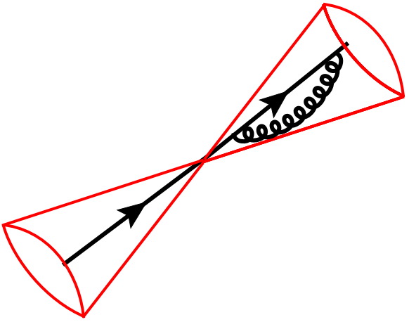
$=\displaystyle\frac{1}{\epsilon}J^{(2)}_{\text{IRC-safe}}-\displaystyle\frac{1}{\epsilon}J^{(2)}_{\text{IRC-safe}}={\color[rgb]{0,0.7,0}\text{finite}}$

+

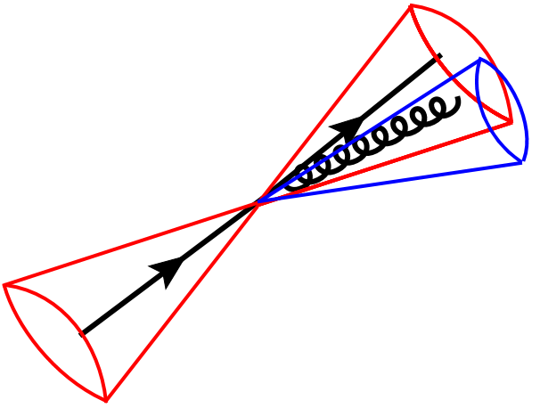
$=\displaystyle\frac{1}{\epsilon}J^{(3)}_{\text{IRC-unsafe}}-\displaystyle\frac{1}{\epsilon}J^{(2)}_{\text{IRC-unsafe}}={\color[rgb]{1,0,0}\infty}$

Figure 1: Importance of the infrared and collinear safety of a jet algorithm. In the top row, an IRC-safe jet definition is used and the corresponding cross section is finite at any perturbative order. In the bottom row, an IRC-unsafe jet definition brakes singularity cancellation between the real and virtual diagrams and leads to an infinite cross section.

Jets are meant to be proxies of the hard partons which participated in the short-distance interaction at early times of a hadron-hadron collision. These hard partons carry large transverse energy, which is subsequently released by consecutive splittings. Because of the soft and collinear enhancements of the QCD branchings, in the majority of cases, the series of emissions does not change direction of the energy flow.

The cross sections in QCD diverge when the angle of emission or the energy of the emitted gluon go to zero. In the perturbative regime, each emission corresponds to the real part of a higher order correction and comes with a power of the strong coupling, ${\alpha_{s}}$. Hence, $n$ emissions contribute to ${{\cal O}\left({\alpha_{s}}^{n}\right)}$ correction. However, the complete ${{\cal O}\left({\alpha_{s}}^{n}\right)}$ result requires also diagrams with up to $n$ loops. And these diagrams come with divergences that match exactly those of the real emissions. Once the real and the virtual contributions at the order ${\alpha_{s}}^{n}$ are added together, the cross section becomes finite up to this order. This intuitively natural results stems from unitarity and was formally proved by Kinoshita, Lee and Nauenberg [47, 48]. The above theoretical mechanism of singularity cancellations is also realised in experiment thanks to the finite energy and angle resolution, which makes the events with ultra-soft or collinear emissions indistinguishable from those with no emissions, the latter corresponding to virtual corrections.

The above mechanism of cancellation of the singularities may not work with a bad choice of an observable and, in our context, a jet definition. The problem is schematically illustrated in Fig. 1. In the top row we see the real and virtual corrections to the dijet production. Each of them is separately divergent, which is denoted by the $1/\epsilon$ pole of dimensional regularization on the right hand side. The red cones represent a jet definition. We see that both the real and virtual diagram are classified as 2-jet configurations, hence the poles are multiplied by the same jet function $J^{(2)}$ (which, in practice, is a definition of an observable) and the divergent terms cancel in the sum leading to a finite result.

This is to be contrasted with the situation depicted in the bottom row of Fig. 1, where a different jet definition was applied to the very same real and virtual diagrams. As we see, now, the real diagram is classified as a 3-jet event while the virtual diagram is still a 2-jet event. This has severe consequences because the poles are now multiplied by different jet functions, respectively $J^{(3)}$ and $J^{(2)}$. Thus, the cancellation of singular terms does not occur, and the final result is infinite. Infinities cannot of course appear in real experimental situations, where they are always regularized by a finite granularity of a detector. Hence, the fact that we obtain a nonsensical theoretical result in the above example comes from the bad choice of a jet definition.

The situation from the top row of Fig. 1 corresponds to the infrared and collinear (IRC) safe jet algorithm, which has a property that the set of hard jets cannot be modified by an arbitrarily collinear or soft emission (either of perturbative origin or coming from non-perturbative dynamics at scales below $\Lambda_{\text{QCD}}$). In general, an IRC-safe observable forms a sum over all states with similar energy flow into the same final state [16]. On the contrary, the jet algorithm used in the bottom row of Fig. 1 is IRC-unsafe, as an arbitrary collinear emission is capable of changing the set of hard jets.

It is clear from the above examples that the IRC-safety of a jet definition is a crucial requirement if we are not to waste the results for higher order corrections to process with jets. Many algorithms used in the past had problems with IRC safety, which were appearing at different levels of perturbative expansion (see [1, 29] for detailed discussions). All modern jet algorithms used at the LHC fully comply with the IRC safety requirement. Hence, they can be used for calculations at arbitrary precision, which then can be meaningfully compared to the experimental results.

2.3 Modern jet algorithms

A comprehensive discussion of all the modern jet algorithms can be found in [29] as well as in the original articles [40, 41, 42, 43, 44, 45, 46]. In order to make our review self-contained, below, we provide a brief summary of the jet algorithms which became standard choices at the LHC.

A complete jet definition consists of the following elements:

Jet definition = jet algorithm + parameters + recombination scheme.

As already mentioned, jet algorithms fall into two classes: the cone algorithms and the sequential-recombination algorithms. Each jet algorithm comes with at least one free parameter. Recombination scheme specifies how the two 4-momenta of particles $i,j$ combine into a 4-momentum of a particle $k$. Currently, one uses almost exclusively the so-called $E$-scheme, where the 4-momenta of $i$ and $j$ are simply added, hence, $p_{k}=p_{i}+p_{j}$.

The cone algorithms represent a top-down approach to jet finding. They were historically first, with the Sterman-Weinberg algorithm [28] for ${e^{+}e^{-}}$, and they were later extensively used at hadron colliders, especially the Tevatron [1]. Most of them were however plagued with the issues of the IRC unsafety [29]. The problems originated from the need to define seeds in order to start an iterative procedure to search for stable cones. Those seed were identified with final state particles. Such procedure is manifestly IRC-unsafe, as an emission of a soft or collinear parton changes the set of initial seeds, which in turn, for a non-negligible fraction of events, leads to a different set of the final-state jets. Resolution of this long-standing problem came with the Seedless Infrared-Safe Cone jet algorithm (SISCone) [44], where an efficient procedure for finding stable cones, without introducing initial seeds, was proposed.

The sequential recombination algorithms dominate almost exclusively in the jet measurements at the LHC. They represent a bottom-up approach by starting to combine the closest particles, according to a distance measure which can be generally written as

$$d_{ij}=\min(p_{Ti}^{2p},p_{Tj}^{2p})\frac{\Delta R_{ij}^{2}}{R^{2}}\,,\qquad\qquad\qquad d_{iB}=p_{Ti}^{2p}\,,$$ (2.1)

where $d_{ij}$ is a distance between the particles $i$ and $j$ and $d_{iB}$ is a distance between the particle $i$ and the beam. The parameter $R$ is called the jet radius and $\Delta R_{ij}^{2}=(y_{i}-y_{j})^{2}+(\phi_{i}-\phi_{j})^{2}$ is the geometric distance between the particles $i$ and $j$ in the rapidity-azimuthal angle plane. The value of the parameter $p$ defines specific algorithm from the sequential-recombination family: $p=1$ for the $k_{T}$ algorithm [40, 41], $p=0$ for the Cambridge/Aachen (C/A) algorithm [42, 43], and $p=-1$ for the anti-$k_{T}$ [46] algorithm.

Given a set of the final-state particles, each procedure of finding jets with the sequential-recombination algorithm consists of the following steps:

1. Compute distances between all pairs of final-state particles, $d_{ij}$, as well as the particle-beam distances, $d_{iB}$, using the measure from Eq. (2.1).

2. Find the smallest $d_{ij}$ and the smallest $d_{iB}$ in the sets of distances obtained above.

   • If $d_{ij}<d_{iB}$, recombine the two particles, remove them from the list of final-state particles, and add the particle ${ij}$ to that list.

   • If $d_{iB}<d_{ij}$, call the particle $i$ a jet and remove it from the list of particles.

3. Repeat the above procedure until there is no particles left.

In spite of the fact that the distance measure of the three algorithms can be written as a single formula (2.1), because of the different values of the power $p$, each of them exhibits a different behaviour. The $k_{T}$ algorithm starts from clustering together the low-$p_{T}$ objects and it successively accumulates particles around them. The C/A algorithm is insensitive to the transverse momenta of particles and it builds up jets by merging particles closest in the $y-\phi$ plane. The anti-$k_{T}$ algorithm starts from accumulating particles around high-$p_{T}$ objects, just opposite to the behaviour of the $k_{T}$ algorithm. In the anti-$k_{T}$ algorithm, the clustering stops when there is nothing within radius $R$ around the hard center. For that reason, anti-$k_{T}$ leads to jets that take circular shapes in the $y-\phi$ plane. This last feature makes the anti-$k_{T}$ algorithm particularly attractive from the experimental point of view. The reason is that jets with regular shapes allow for reliable interpolation between detector regions separated by dead zones. That is why the anti-$k_{T}$ algorithm became a default choice at the LHC.

All the algorithms discussed in this section are available within the FastJet package [49].

2.4 Jet mass

Amongst a number of properties of a jet, its mass turns out to be especially important in numerous contexts. In the approximation of massless QCD partons, the jet mass arises due to its substructure. In pure QCD, the substructure comes from radiation of gluons and quarks. However, in processes involving a hadronic decay of a heavy object of mass $m$ and $p_{T}\gg m$, the decay products will also end up in a single jet building up its mass.

If a jet $J_{12}$ is obtained from clustering of the two subjets $J_{1}$ and $J_{2}$, its exact mass is given by [50]

$$m_{12}^{2}=2m_{T1}m_{T2}\cosh(y_{2}-y_{1})-2p_{T1}p_{T2}\cos(\phi_{2}-\phi_{1})+m^{2}_{1}+m^{2}_{2}\,,$$ (2.2)

where $m_{Ti}=\sqrt{m_{i}^{2}+p_{Ti}^{2}}$ are the transverse masses of the subjets, while $p_{T1}$, $p_{T2}$ and $y_{1}$, $y_{2}$ are, respectively, the subjets’ transverse momenta and rapidities. In the limit of $m_{i}\ll p_{Ti}$ and $R\ll 1$, the above formula reduces to

$$m^{2}_{{12}}\simeq m^{2}_{1}+m^{2}_{2}+z(1-z)\,p_{T{12}}^{2}\Delta_{12}^{2}\,,$$ (2.3)

where $p_{T{12}}$ is the transverse momentum of the jet formed by recombination of particles 1 and 2, while $\Delta_{12}$ and $z$ are given by

$$\Delta_{12}=\sqrt{(y_{1}-y_{2})^{2}+(\phi_{1}-\phi_{2})^{2}}\equiv xR\,,\qquad\qquad z=\frac{\min(p_{T1},p_{T2})}{p_{T1}+p_{T2}}\,.$$ (2.4)

Jet mass is an infrared and collinear safe quantity that can be calculated order by order in perturbation theory. Because of the soft and collinear singularities of the QCD matrix element for gluon emission, the distribution of masses, $m_{J}$, of the QCD jets receives strong enhancement at low values of $m_{J}$. At the lowest, non-trivial order, the approximate result for the mass distributions of QCD jets is given by $\frac{d\sigma}{dp_{TJ}dm_{J}}\propto\alpha_{s}(p_{TJ})\frac{4C_{i}}{\pi m_{J}}\ln\left(\frac{R\,p_{TJ}}{m_{J}}\right)$ [51], where $C_{i}$ is the colour factor of the initiating parton and $R$, $p_{TJ}$, $m_{J}$ are the jet’s radius, transverse momentum and mass, respectively. The higher order terms are enhanced by further powers of $\ln\frac{R\,p_{TJ}}{m_{J}}$.

Contrary to the case of QCD, the distribution of jets coming from a decay of a heavy object is flat in $z$ and therefore, the mass distribution of such jets is peaked around the mass of the heavy object which originated them. This will be discussed further in Section 2.7.

2.5 Jet area

It is intuitive to think that the larger the jet, the more its transverse momentum is susceptible to contamination from soft radiation, such as UE or PU. This is just because the jets will capture the incoherent radiation proportionally to their area, hence, larger jets will be more affected (in absolute terms). The naive geometrical expectation for the area of a jet with radius $R$ is $\pi R^{2}$. A closer investigation reveals that the actual area of a jet is in most cases different and that there is some freedom in its definition.

A quantitative discussion of jet areas started with the work of Ref. [52] were two types, the passive and the active area, were introduced. They both use the concept of ghosts, $\{g_{i}\}$, i.e. infinitely soft particles which are added to the set of the final state particles $\{p_{k}\}$. If the whole ensemble $\{p_{k},g_{i}\}$ is clustered with an IRC-safe algorithm, the resulting set of jets $\{J_{n}\}$ will be identical to that from clustering just the physical particles $\{p_{k}\}$.

The scalar passive area of the jet $J$ is defined as the area of the region in the $y-\phi$ plane in which the single ghost particle, $g$, is clustered with $J$

$$a(J)\equiv\int dy\,d\phi\,f(g(y,\phi),J),\hskip 30.0ptf(g,J)=\bigg{\{}\begin{array}[]{cl}1&{\rm for\ }g{\rm\ clustered\ with\ }J\\ 0&{\rm for\ }g{\rm\ not\ clustered\ with\ }J\end{array}\,.$$ (2.5)

A 4-vector version of the passive area is introduced in a similar way [52].

The passive area (2.5) provides a measure of the susceptibility of the jet to soft radiation in the limit in which this radiation is pointlike. For a 1-particle jet $J_{1}$, $a(J_{1})=\pi R^{2}$, for all four jet clustering algorithms: $k_{T}$, C/A, anti-$k_{T}$ and SISCone. For a 2-particle jet, the passive area starts to depend on the jet definition and the geometrical distance between particles. The analytic results for strongly ordered transverse momenta were obtained in Ref. [52], and, in Ref. [53], they were generalized to the case with arbitrary transverse momenta.

The active area has more physical relevance and it is defined with a dense coverage of ghosts, randomly distributed in the $y-\phi$ plane. If the number of ghosts from a particular ghosts ensemble $\{g_{i}\}$ clustered with the jet $J$ is ${\cal N}_{\{g_{i}\}}(J)$, and the number of ghosts from this ensemble per unit area is $\nu_{\{g_{i}\}}$, then the active scalar area is given by

$$A(J)\equiv\lim_{\nu_{g}\to\infty}\left\langle A(J\,|\,\{g_{i}\})\right\rangle_{g}\,,\qquad A(J\,|\,\{g_{i}\})=\frac{{\cal N}_{\{g_{i}\}}(J)}{\nu_{\{g_{i}\}}}\,,$$ (2.6)

where $\langle\ldots\rangle_{g}$ denotes the average over many ensembles of ghosts with the number of ghosts in each ensemble $\nu_{g}\to\infty$. Similarly, the 4-vector active area may be defined [52].

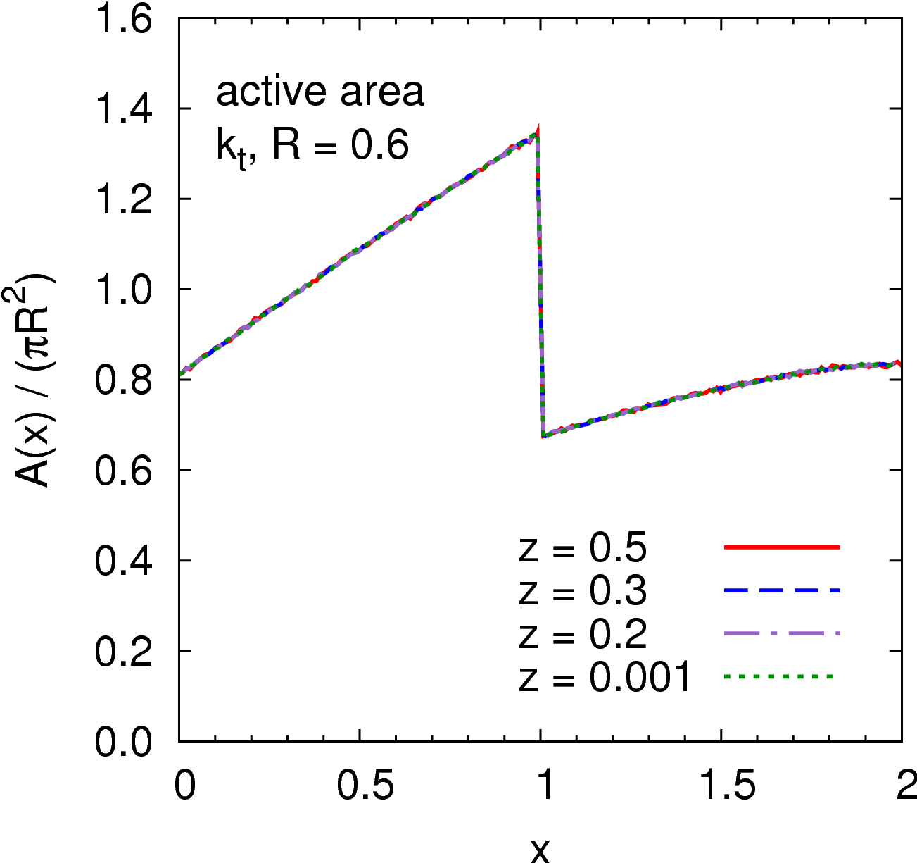
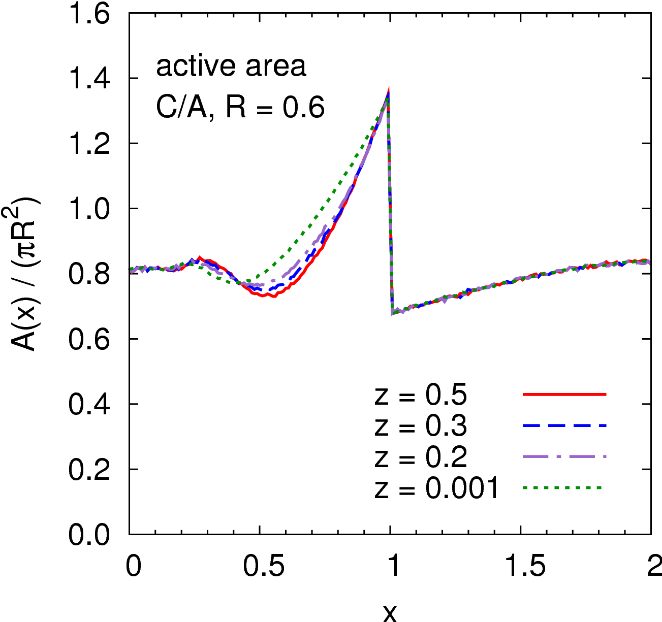
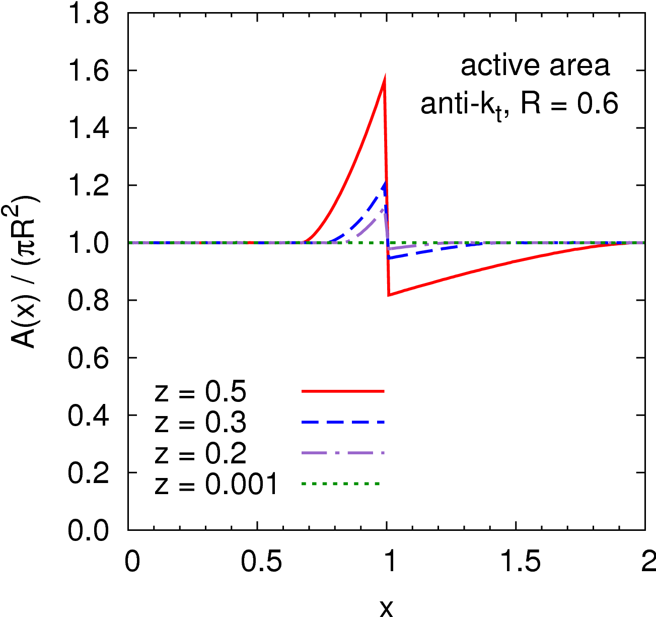
Figure 2: Active areas of the hardest jet for the system of two particles separated by the distance $xR$, defined in Eq. (2.4) together with the asymmetry parameter $z$. Figure from Ref. [53].

Fig. 2 shows the active area of the hardest jet in a 2-particle system with the geometrical separation between the particles, $\Delta_{12}\equiv xR$, and the relative transverse momenta of the constituents, $z$, given in Eq. (2.4). We see that the “non-conical algorithms”, i.e. $k_{T}$, which start from clustering ghosts among themselves, and C/A, exhibit virtually no dependence on the $z$ parameter, which measures how much of the total jet’s transverse momentum is taken by the softer particles. On the contrary, the active area of the “conical”, anti-$k_{T}$ algorithm depends quite strongly on the $p_{T}$ asymmetry of the constituents when those constituents are separated by $\simeq R$.

In all three cases shown in Fig. 2, the areas increase with the constituent separation for $x<1$ ($\Delta_{12}<R$). In this region, the two particles form a single jet. For $x>1$, each particle is clustered into a separate, 1-particle jet but because the distance between the particles is smaller than $2R$, the area of the hardest jet is smaller than that of a 1-particle jet in a single-particle event. As $x\to 2$, however, the hardest jet area tends to the result for 1-particle active area.

2.6 Jet mass area

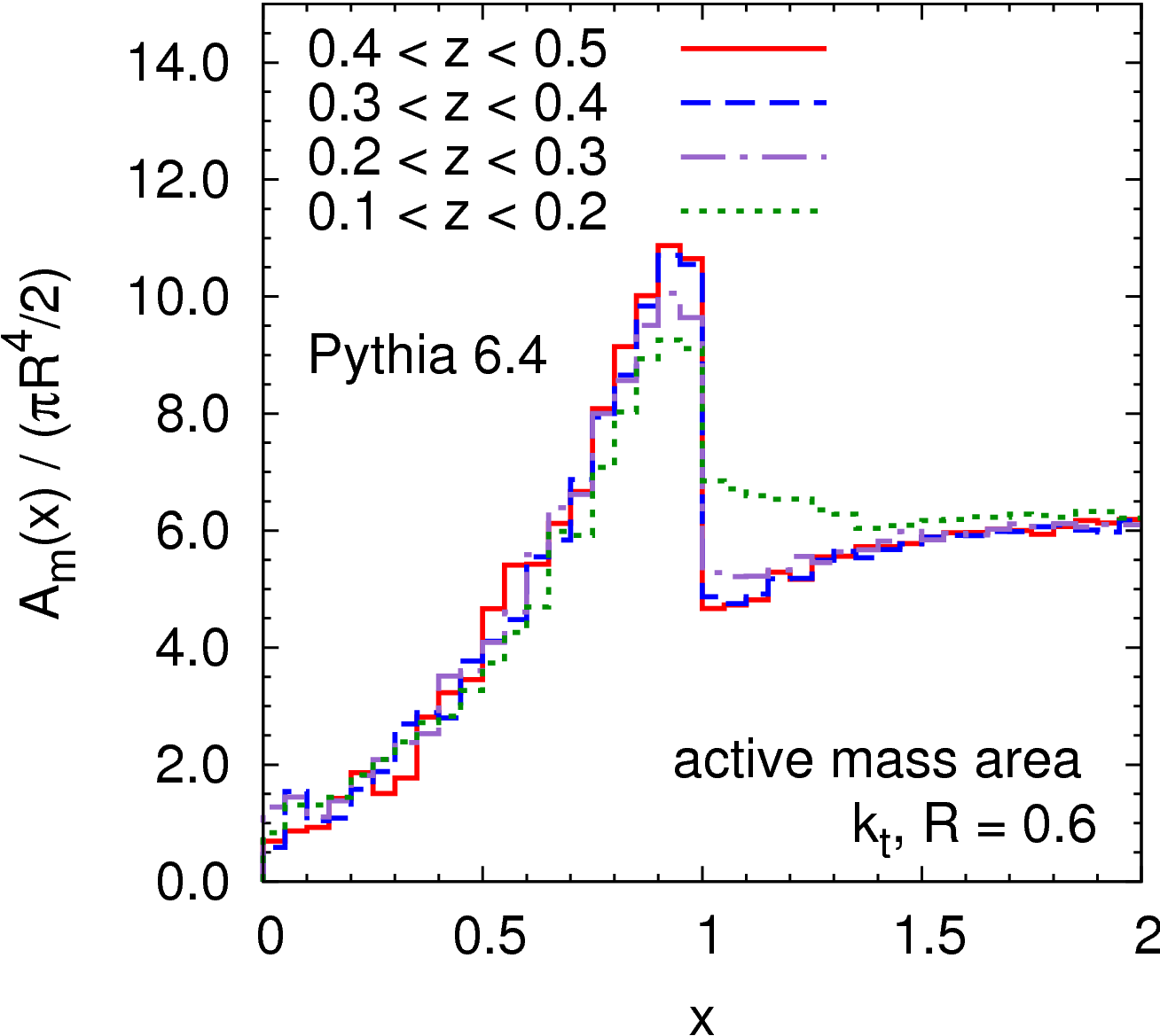
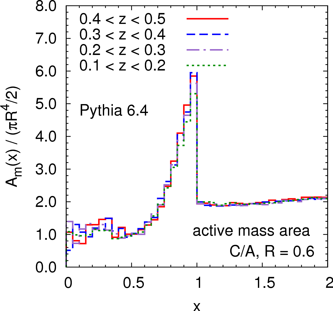
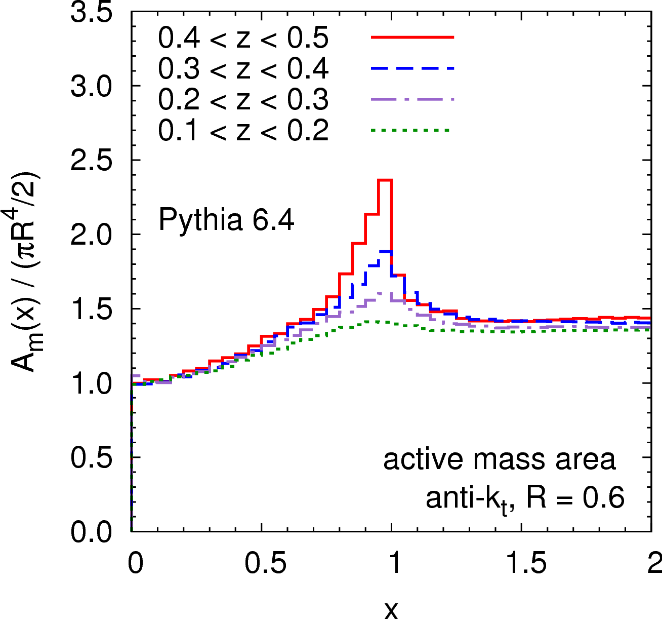
Figure 3: Active mass areas of the hardest jet from dijets events simulated with Pythia. The distance $x$ and the asymmetry parameter $z$, defined in Eq. (2.4), were obtained using the two hardest subjets. Figure from Ref. [53].

Just like the value of the jet area specifies susceptibility of jet’s transverse momentum to incoherent radiation, the value of the mass area specifies how much that radiation affects the jet mass. It can be also defined in the passive and active variants, of which the latter has more relevance for jets produced at hadron colliders.

The active mass area is defined as [53]

$$A_{m}(J)\equiv\lim_{\nu_{\{g_{i}\}}\to\infty}\left\langle\frac{m^{2}_{J{\{g_{i}\}}}-m^{2}_{J}}{\nu_{\{g_{i}\}}\left\langle\smash{p_{tg}}\right\rangle p_{TJ\{g_{i}\}}}\right\rangle_{g}=\frac{2}{p_{TJ}}\,p^{\mu}_{J}A_{\mu}(J)\,,$$ (2.7)

where $m_{J}$ is a mass of the pure jet $J$ and $m_{J{\{g_{i}\}}}$ is a mass of the jet consisting of $J$ and a dense coverage of ghosts from the random ensemble $\{g_{i}\}$. The last equation holds when all jet constituents are massless, and $A_{\mu}(J)$ is a 4-vector, active jet area.

Analytic study of the active jet areas for the 2-particle jets, as well as their passive analogues, can be found in Ref. [53]. The 1-particle jet passive mass area is equal to $\pi R^{4}/2$ and this is how all the active and passive mass areas scale. The qualitative behaviour of the mass areas of the 2-particle jets is very similar to that found for jet areas. The $x$ dependence follows that of Fig. 2 and $z$ dependence is again very weak for $k_{T}$ and C/A and fairly sizable for anti-$k_{T}$.

In Fig. 3 we show the analogue of Fig. 2 for the active mass areas but, this time, the hardest jet comes from full Pythia6 [54] simulation of dijets events at hadron level, with the underlying event switched off. The results from Fig. 3 are in qualitative agreement with those for the active mass areas of 2-particle jets and follow the shapes of the jet areas of Fig. 2. The general pattern of growth of the mass area with $x$ and then a drop at $x\simeq 1$ is well observed. Also, the sensitivity to the $z$ value is similar to that found in Fig. 2: low for $k_{T}$ and C/A while noticeable for anti-$k_{T}$.

Jets from full simulation are of course much more complex, which leads to some differences with respect to a simple 2-particle picture. We see, for example, that the mass areas from the $k_{T}$ algorithm are significantly larger than those from C/A and anti-$k_{T}$. This is related to a larger scaling violation in the case of $k_{T}$, which means that even collinear emissions can lead to a significant increase of the mass area [53]. Another complication with respect to the simple 2-particle jets is that, in the latter case, the hardest jet area and mass area always return to the 1-particle jet result as $x\to 1$. In real-life jets they stay much bigger since, with many particles in the final state, widely separated subjets develop their own substructure and cannot be any longer approximated by a single, massless particle.

2.7 Jet substructure

It is apparent from our discussion so far that jets have a very rich substructure. Patterns of radiation found inside a jet carry important information about its origins. The studies of jet substructure have become a separate, and by now well developed, field of research. It is therefore impossible to do justice to all important results that appeared over the last yeas as that alone would require a dedicated review article. We shall however briefly sketch the main ideas behind the studies of jet substructure and describe the most important techniques.

The main motivation behind the studies of a structure of radiation inside a jet is a potential enhancement of the signal vs background discrimination. Suppose that we find a jet with certain mass and transverse momentum and with two well defined subjets. Those subjets can be, to a first approximation, modelled as QCD partons that originated from a single vertex. Depending on the nature of this vertex, the outgoing partons share the momentum of the incoming particle in a very different way. In the collinear limit we have: $P(z)\propto 1$ for the decay of a heavy boson $V\to q{\bar{q}}$ but $P(z)\propto\frac{1+z^{2}}{1-z}$ for the QCD splitting $q\to qg$. Here, $P(z)$ is a splitting probability with the momentum shared between the outgoing partons in fractions $z$ and $1-z$. This simple observation opens a possibility of discriminating between jets coming from decays of heavy, colourless objects, and those originating from pure QCD branchings. In the first case, the two subjets will share the momenta of a jet symmetrically, whereas in the second case, one of the subjets will be much harder than the other. Similar considerations apply to the angle between the two subjets. In majority of cases, this angle will be larger for $V\to q{\bar{q}}$ than for $q\to qg$, as the latter splitting is collinearly enhanced.

The angle and momentum enter the distance measure of the $k_{T}$ algorithm, c.f. Eq. (2.1). Hence, by taking one step back in the clustering of a jet, we obtain two subjets which we can treated as proxies of the partons originating from the relevant splitting (i.e. the one that builds up most of the jet mass [50]). This procedure was first used in Ref. [55] in the study of $H\to WW$ followed by one $W$ decaying leptonically and the other hadronically. If the $p_{T}$ of a lepton from one $W$ is large, the hadronic decay products from the other $W$ will end up in a single, fat jet. The $k_{T}$ measure distance between the two hardest subjets, $d_{12}$, will be on average substantially larger if those jet come from the $W\to jj$ decay than if they come from a QCD splitting. Therefore, by rejecting the events with $d_{12}<d_{\text{cut}}$, a procedure generally called tagging, one can significantly improve the signal to background ratios. Similar techniques were proposed later to study the $WW\to jj+\l\nu$ process [56] and to enhance SUSY signals [57].

The above ideas have been developed and refined in the BDRS study of Ref. [58] focused on suppressing large backgrounds to the associated Higgs production with a subsequent decay to the $b{\bar{b}}$ pair, $pp\to ZH\to l^{+}l^{-}b{\bar{b}}$. Here, the C/A algorithm has been used to study the substructure of the fat jet, $J$, containing the two bottom quarks, expected to enter the two subjets, $J_{1}$ and $J_{2}$, of which $J_{1}$ is heavier.

Contrary to the $k_{T}$ algorithm, C/A does not necessarily end the clustering with the relevant splitting. Therefore, to identify the latter, the mass drop condition has been introduced in addition to the asymmetry cut. The two conditions read

$$\frac{m_{J_{1}}}{m_{J}}<\mu_{\text{cut}}\,,\qquad\text{and }\qquad\frac{\min\left(p_{TJ_{1}}^{2},p_{TJ_{2}}^{2}\right)}{m_{J}^{2}}\Delta^{2}_{12}>y_{\text{cut}}\,,$$ (2.8)

with $\Delta_{12}$ defined as in Eq. (2.4). If both conditions are met, i.e. the splitting $J\to J_{1}J_{2}$ is not too asymmetric and the unclustering leads to a significant mass drop, than the branching is identified as the $H\to b{\bar{b}}$ decay, with each of the $b$ quarks entering the subjet $J_{1}$ and $J_{2}$, respectively. Otherwise, $J$ is redefined as $J_{1}$ and the whole procedure is iterated.

The advantage of using the C/A algorithm with the mass drop is that it already cleans a jet from incoherent radiation as it makes its way to the relevant splitting. To further improve its performance, the BDRS procedure has been supplemented with one additional step, dubbed filtering, in which the jet is reclustered with a much smaller radius, $R_{\text{filt}}$, and only the $n$ hardest subjets are taken for mass reconstruction. This helps to remove even more of the unwanted contamination from the underlying event while keeping the most important perturbative radiation from the Higgs decay products. The original analysis of Ref. [58] used $n=3$ but the filtering procedure can be defined with an arbitrary number of subjet taken for mass reconstruction [59].

In Ref. [60], a modification of the BDRS tagger has been proposed, in which, in the case when the conditions from Eq. (2.8) are not met, the $J$ is redefined not as $J_{1}$ but as this of the two subjets, $J_{1}$ and $J_{2}$, whose transverse mass, $m_{TJ_{i}}^{2}=m^{2}+p_{TJ_{i}}^{2}$, is the largest. Such a tagger was called the modified mass drop tagger (mMDT). This modified version turns out to perform better on a special class of configurations in which a massless parton emits a soft gluon that subsequently splits collinearly into a $q{\bar{q}}$ pair. Because the first parton is massless, the BDRS tagger would choose the $g\to q{\bar{q}}$ branch for further iterations, even though this branch comes from a soft gluon. The modification made in mMDT fixes the above feature by elimination of sensitivity to soft divergences and renders the tagger that is better-behaved from the point of view theoretical calculations [60].

In general, procedures aimed at cleaning the incoherent radiation from a jet are called grooming techniques. Other, by now well established, examples include pruning [61, 62], trimming [63] and $N$-subjettiness [64, 65].

Pruning [61, 62] was designed to identify signal events with heavy objects decaying hadronically and to clean them from incoherent radiation. The procedure modifies jet substructure in order to reduce the systematic effects that obscure the reconstruction of hadronic heavy objects. It takes the constituents of a jet and puts them through a new clustering procedure in which each of the branchings is requested to pass a pair of cuts on kinematic variables. If the cuts are not passed, then the recombination is vetoed and one of the two branches is discarded. The conditions for each recombination $ij\to k$ are

$$\frac{\min(p_{Ti},p_{Tj})}{p_{Tk}}>z_{\text{cut}}\qquad{\rm and}\qquad\Delta_{ij}<D_{\text{cut}}\,,$$ (2.9)

where $D_{\text{cut}}$ is chosen dynamically according to $D_{\text{cut}}=2D\frac{m_{J}}{p_{TJ}}$ and the parameters $z_{\text{cut}}$ and $D$ are optimized based on Monte Carlo simulations. If both conditions given in Eq. (2.9) are satisfied, the merging takes place, otherwise, the softer branch is discarded.

Trimming procedure [63] takes a jet obtained with the original definition which used the size $R$ and reclusters its constituents into subjets employing an algorithm with the smaller jet radius $R_{\text{sub}}$. In the next step, only the subjets whose transverse momenta that satisfy the condition

$$p_{Ti}>f_{\text{cut}}\,\Lambda_{\text{hard}}\,,$$ (2.10)

are kept and they are subsequently recombined into the new, trimmed jet. In the condition of Eq. (2.10), $f_{\text{cut}}$ is a dimensionless parameter, optimized based on simulations, and $\Lambda_{\text{hard}}$ is a hard scale characteristic to a given process.

N-subjettiness [64] exploits the fact that the pattern of the hadronic decay of a heavy object is characterised by the presence of concentrated energy depositions corresponding to the decay products. On the contrary, a QCD jet represents a more uniformly spread energy configuration. The inclusive jet shape, $N$-subjettiness, is defined, in its generalized version derived in [65], as

$$\tau_{N}=\frac{1}{d_{0}}\sum_{k}p_{Tk}\min\left((\Delta R_{1k})^{\beta},...,(\Delta R_{Nk})^{\beta}\right)\,,$$ (2.11)

where $k$ runs over the constituent particles in the jet, $\Delta R_{jk}=\sqrt{(\Delta y)^{2}+(\Delta\phi)^{2}}$ is a distance between the constituent $k$ and the subjet $j$, $\beta$ corresponds to an adjustable parameter called the angular weighting exponent, and the normalization factor reads $d_{0}=\sum_{k}p_{Tk}R^{\beta}$, with $R$ being the jet radius.

The variable $\tau_{N}$ approaches 0 when the constituents of the jet are aligned along $N$ directions. The latter correspond to $N$ subjets. On the opposite end, large values of $\tau_{N}$ signal that the number of distinct subjets is greater than $N$. Hence, the ratio $\tau_{N}/\tau_{N-1}$ turns out to be a useful discriminating variable. For example, in the case of two-prong hadronic decays, $\tau_{2}/\tau_{1}$ is on average smaller for the signal than for the background events.

Many different taggers and groomers appeared since the first proposals briefly described above. Because of space limits, we cannot even mention all of them here. Instead, we refer to the recent reports following the topical BOOST conference [30, 31], where the Reader can find most of the essential information and references.

Let us conclude by noting that, after the initial stage characterized by developments of new taggers and groomers, and essentially Monte Carlo-based optimization of their parameters, the efforts of the community turned into comparisons between different tools [66, 50] and into gaining their analytic understanding [67, 60, 68, 69, 70].

3 Factorization in hadroproduction of jets

Jets are defined as collimated streams of particles carrying sizable energy in the transverse direction, hence, they are genuinely hard objects, which can be treated by perturbative QCD. However, even though jets originate from collisions of highly energetic hadrons, the hadrons themselves are characterized by low transverse scales, related to their masses, only up to a few times larger than $\Lambda_{\text{QCD}}$ . This introduces a hierarchy of scales from $\Lambda_{\text{QCD}}$ to $p_{T,\text{jet}}$, with the latter varying between tens of GeV and several TeV.

Such a large span of scales creates a very rich dynamics, which poses serious calculational challenge. Moreover, the low-scale dynamics of hadron binding cannot be approached by perturbative QCD. It turns out however, that the problem can be handled by extracting dominant contributions at various scales, the so called, regions, and by factorizing the cross sections into the short- and long-distance pieces, which can then be calculated separately.

The factorization, which is the subject of this section, is at heart of all calculations at hadron colliders. Even though it has been intensely studied since the very beginnings of QCD, with the seminal works of Refs. [71, 72, 73, 74, 75, 76, 77], it is rigorously proven only for a handful of processes and for the cases of sufficiently inclusive observables.

3.1 Collinear factorization

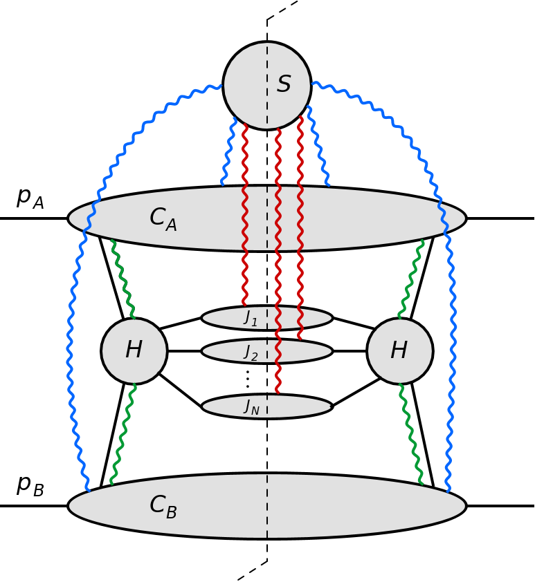
Figure 4: The most general leading pinch singular surface diagram for hadron-hadron collision.

Figure 5: Factorized form of the cross section in hadron-hadron collision.

A general cut diagram for the hadron-hadron scattering is shown in Fig. 5. It involves a low scale $m\sim\Lambda_{\text{QCD}}-1\,\text{GeV}$, which is in a typical range of hadron masses, and the hard scale, $Q$, which is of the order of jet’s transverse momentum. We denote the ratio of the two scales by $\lambda=m/Q$. In general, one is interested in the expression for the cross section corresponding to the diagram of Fig. 5 in the limit $\lambda\to 0$.

It turns out that, in the above limit, the integral over loop momenta is divergent. Some of those divergences are only apparent and can be removed by deformation of the integration contours into the regions of the complex plane where the integrals are finite. There is however an entire class of singularities that, in the limit $\lambda\to 0$, pinch the integration contour such that it cannot be deformed. Those integration surfaces, called the leading pinch singular surfaces (LPSS), give the dominant contribution to the cross section, the so-called leading twist, and all the other terms are suppressed as powers of $m/Q$ and hence contribute at higher twist.

Fig. 5 shows the most general LPSS diagram divided into several classes of subdiagrams, each of which corresponds to a different leading region:

• $C_{A}$ and $C_{B}$ are the collinear subgraphs and characterize the incoming partons and the corresponding beam remnants after the hard reaction. The particles in the $C_{A,B}$ subgroups belong to the collinear region, which means that their momenta, in notation $p_{\mu}=(p_{+},p_{-},p_{T})$, scale as

  $$p_{C_{A},\mu}\sim Q\,(1,\lambda^{2},\lambda)\,,\qquad\qquad\qquad p_{C_{B},\mu}\sim Q\,(\lambda^{2},1,\lambda)\,.$$ (3.1)

• $H$ is the hard subgraph, with the interactions happening at the hard scale $Q$ and the momentum scaling

  $$p_{H,\mu}\sim Q\,(1,1,1)\,.$$ (3.2)

• $J_{1},J_{2},\ldots,J_{N}$ are the final-state jets created after the hard interaction that happened in $H$. The jets are build-up from particles collinear to the momenta going out of the hard part $H$.

• $S$ is the soft subgraph connecting to other subdiagrams with soft gluons whose momenta scale as

  $$q_{S,\mu}\sim Q\,(\lambda,\lambda,\lambda)\,.$$ (3.3)

The above subgraphs are in general connected by quark and gluon lines. One can show, however that all connections except those involving one collinear and an arbitrary number of longitudinally polarized gluons between the collinear and the hard subgraphs, or the soft gluons between the soft and the collinear, or the soft and the final state jet subgraphs, contribute only to the higher twist [78]. On the contrary, any number of the remaining gluons connections, denoted by wavy lines in Fig. 5, will survive at the leading twist and therefore must be resummed.

In simple theories, like the asymptotically free, non-gauge $\phi^{3}$ theory in 5+1 dimensions, contrary to QCD, there are no soft gluon connections between the leading subgraphs. Moreover, only one collinear parton from the collinear part connects to the hard part. Hence, the contribution to each leading diagram automatically takes the form of the product of the leading subgraphs: the hard part and the collinear parton distribution functions. This is what we call topological factorization [75]. As shown in Fig. 5, topological factorization does not occur in QCD because of the soft gluon connections between various parts of the diagram, as well as the longitudinal gluons connecting the collinear and the hard part. All the diagrams with multiple gluonic connections contribute to the leading twist and that is why factorazibility of QCD is a highly non-trivial feature: In order to arrive at the factorization formula, one needs to show that the effects of the soft and longitudinal gluons cancel or can be resummed.

The hadronic cross section factorizes if it can be written in the form

$$d\sigma=\sum_{a,b}f_{a/A}\otimes f_{b/B}\otimes H_{ab}\otimes S_{ab}\otimes J_{1}\otimes\ldots J_{N}+\text{p.s.c.}\,,$$ (3.4)

where $f_{a/A}$ and $f_{b/B}$ are the collinear (integrated) parton distributions functions (PDFs), corresponding to the collinear subgraphs and the rest of the notation follows that of Fig. 5. The formula sums over all parton species and the extra term ”p.s.c” denotes the power-suppressed corrections (of higher twist), which are multiplied by extra powers of $1/Q$ with respect to the leading part.

The PDFs, $f_{a/A}$ and $f_{b/B}$, are process-independent, whereas the sets of the soft, $S_{ab}$, and the hard, $H_{ab}$, functions are process-specific. The latter is also referred to as the partonic cross section and, in the perturbative regime, i.e. for $Q\gg\Lambda_{\text{QCD}}$, it can be calculated order by order in powers of the strong coupling

$$H_{ab}=H_{ab}^{\text{LO}}+\left(\frac{{\alpha_{s}}(\mu_{R}^{2})}{2\pi}\right)H_{ab}^{\text{NLO}}+\left(\frac{{\alpha_{s}}(\mu_{R}^{2})}{2\pi}\right)^{2}H_{ab}^{\text{NNLO}}+\ldots\,.$$ (3.5)

Let us now sketch the proof of Eq. (3.4). In the general diagram of Fig. 5, various sub-graphs, corresponding to interactions happening at different energy scales, are connected. The aim of the factorization program is to show that many of these connections disappear at leading twist and the expressions corresponding to Fig. 5 can be written as a simple convolution of the hard, the soft and the collinear functions.

QCD factorization is an enormously vast subject with plenitude of subtelties. Our discussion presented below can be only brief on some of those issues. We shall however try to signal the most important ingredients that enter proofs of factorization. More details can be found in the references provided in the remaining part of this section. In addition, we point the Reader to the nicely structured overview of the different steps taken in factorization proofs presented in Ref. [79], where many issues are clarified in order to prove the factorization in the very non-trivial case of the double Drell-Yan process.

In gauge theories, like QCD, there are essentially three challenges that need be addressed in order to demonstrate the factorization property of the cross section (3.4). They correspond to the following connections, which can spoil the factorization  [75]:

1. Soft-gluon connections between the wide angle jets in the hard subdiagram (red in Fig. 5).

2. Soft-gluon connections between the collinear subgraphs $C_{A}$ and $C_{B}$ via the soft function $S$ (blue in Fig. 5). These are the interactions between the spectator particles.

3. Longitudinally-polarized-gluon connections between the collinear subgraphs $C_{A,B}$ and the hard part $H$ (green in Fig. 5).

The proof of factorization for the soft gluon connections of the first and the second type proceeds via deformation of the contour of integration in the complex plane of the soft gluon momenta such that one of the longitudinal components dominates along the entire integration path. Subsequently, one uses the non-abelian Ward identities (hence, gauge invariance) to show that the corresponding contribution either vanishes or factorizes.

However, in some cases, the above procedure encounters extra difficulty because the connecting gluons are pinched in the so-called Glauber region [72, 75], which makes the necessary contour deformation impossible. Let us now take a closer look at this problematic issue.

3.1.1 Glauber region

Consider the soft gluon with momentum $q$, c.f. Eq. (3.3), coupling to the massless quark line with momentum $p$ collinear to $p_{A}$, hence scaling similar to Eq. (3.1). This leads to appearance of the propagator with the following denominator

$$(p+q)^{2}+i\epsilon\simeq 2p^{+}q^{-}+q^{+}q^{-}-q_{T}^{2}+i\epsilon\,.$$ (3.6)

By studying the integral over $q^{-}$, we notice that gluons from the soft region satisfy

$$p^{+}q^{-}\sim\lambda\quad\gg\quad q^{+}q^{-},\,q_{T}^{2}\sim\lambda^{2}\,.$$ (3.7)

Hence, the minus component of the gluon’s 4-momentum dominates and $(p+q)^{2}\simeq 2p^{+}q^{-}+i\epsilon$.

If we now go to the rest frame of the incoming hadron $A$, which travels along the plus direction, the polarization vector of the soft gluon will lie, to a good approximation, in the minus direction, $\epsilon_{-}\gg\epsilon_{+},\epsilon_{T}$, and, because of Eqs. (3.3) and (3.7), also the minus component of the gluon’s 4-momentum will dominate. Hence, we have $\epsilon_{\mu}\propto q_{\mu}$, which implies that the gluon arises from a pure gauge potential. Such a contribution can be eliminated by using gauge invariance.

However, a complete integral over $q^{-}$ requires us to go to the lower limit of $q^{-}$, where the relations (3.3) and (3.7) are not satisfied but, instead, we have $p^{+}q^{-}\sim\lambda^{2}\sim q_{T}^{2}$, which corresponds to

$$q^{+}q^{-}\ll q_{T}^{2}\,.$$ (3.8)

This is the so-called Glauber region [72, 75] or the Coulomb region [74, 80, 81] in which the components of the gluon’s 4-momentum are not comparable, as assumed in Eq. (3.3), but the longitudinal components are much smaller than the transverse one. The gluons from the Glauber region are important in various contexts. For example, as discussed in Ref. [82], they give rise to the Lipatov vertex and emergence of the BFKL equation in SCET. The Glauber region is not displayed in Fig. 5 and, in fact, the contributions from that region must vanish in order for the factorization procedure to be successful.

This is because, in the Glauber region, the propagator (3.6) has a pole at $q^{-}\sim q_{T}^{2}/(2p^{+})-i\epsilon\sim m^{2}/(2Q)-i\epsilon$ and the above gauge-invariance arguments cannot be used. If all such poles lie in the same part of the imaginary plane, the integration contour may be deformed into the opposite part such that it is moved out of the Glauber region restoring the relation (3.7). However, if the poles are distributed on both the positive and the negative half of the imaginary plane, the integration contour is pinched in the Glauber region and the cross section does not factorize.

The collinear factorization is rescued from the soft gluons pinched in the Glauber region by the sum over final states. It turns out that, after such a sum is performed, the soft gluon connections between the final state jets $J_{i}$ (red lines in Fig. 5) vanish [75, 77]. This cancellations between graphs takes place because of unitarity, as those interactions happen long after the hard process.

It is important to note that canceling of the final state interactions does not happen only in the fully inclusive cross sections but it occurs also in the jet production cross sections. This is because the hard final state jets are well separated in space and they cannot meet again to produce another hard scattering. Therefore, the interactions between the final state jets can occur only via soft gluons. Hence, the same line of arguments can be applied to jet final states and the soft divergencies will cancel in the sum [83, 84]. Regarding the collinear emissions from the hard final state partons, they are compensated by virtual corrections, for the IRC jet definitions, as discussed in Section 2.2, a feature guaranteed by the KLN theorem [47, 48].

As for the soft connections between the collinear subgraphs, $C_{A}$ and $C_{B}$, i.e. blue lines in Fig. 5, the pinches, which prevented us from deforming the contour away from the Glauber region, disappear after the sum over final states and the deformation is possible. That allows one for application of the non-abelian Ward identities, which then turn the $S-C_{A,B}$ connections into connections between the soft function $S$ and the Wilson lines and that part of the formula factorized from the rest. This is illustrated in Fig. 5 and can be understood by a classical analogy of $C_{A}$ passing through a soft colour filed of $C_{B}$. Since the gluons are very soft, they correspond to interactions between partons in the subgraphs $C_{A}$ and $C_{B}$ long before the hard scattering. But the soft gluons cannot resolve the partons inside the hadron, hence, the subgraph $C_{A}$ appears as a colour singlet and the soft gluons cannot couple to it. This is a manifestation of unitarity.

Thus, the first two problems from the list on page 3.1 are solved. We are now left with the third problem, i.e. the longitudinally polarized gluons connecting $H$ with $C_{A}$ and $C_{B}$, which we discuss in the next subsection.

3.1.2 Parton distribution functions and gauge links

The third issue is solved by using gauge invariance and absorbing the longitudinal gluons into the parton distribution functions via the so called gauge links. More specifically, eikonal propagators can be used for gluons linking the collinear and the hard part, i.e. green gluons in Fig. 5 and then the non-abelian Ward identities allow one to show that the gluons from $C_{A}$ and $C_{B}$ effectively connect to the Wilson line, represented as double line in Fig. 5, which then factorizes from the rest of the diagram. Physically, that comes from the fact that collinear gluons cannot resolve any transverse structure of $H$ and are only sensitive to its longitudinal components. Hence, $H$ appears to those gluons as a Wilson line.

The above procedure leads to the following, gauge invariant definitions of the parton distribution functions for a quark and a gluon [73, 85, 77]

$$f(\xi)_{q/h} =\int\frac{dw_{-}}{2\pi}e^{-i\xi P^{+}w_{-}}\langle P|\overline{\Psi}_{q}(0,0,\mathbf{0}_{T})\,{\cal W}^{n}(0;w_{-})\frac{\gamma^{+}}{2}\Psi_{q}(0,w_{-},\mathbf{0}_{T})|P\rangle\,,$$ (3.9a)

$$f(\xi)_{g/h} =\int\frac{dw_{-}}{2\pi\xi P^{+}}e^{-i\xi P^{+}w_{-}}\langle P|F^{+j}_{a}(0,0,\mathbf{0}_{T}){\cal W}^{n}_{ab}(0;w_{-})F^{+j}_{b}(0,w_{-},\mathbf{0}_{T})|P\rangle\,,$$ (3.9b)

where $\Psi_{q}$ is a Dirac field of a quark $q$ and $F^{ij}_{a}$ is a gluon field-strength tensor.

The object ${\cal W}^{n}(0;w_{-})$ in the above expressions is called the Wilson line (double line in Fig. 5). It effectively resums all exchanges of the longitudinal gluons between the hard part and the collinear part. The general form of the Wilson line reads

$${\cal W}^{C}(a;b)={\cal P}\exp\left[-ig\int_{C}ds_{\mu}A^{\mu}\right]\,,$$ (3.10)

where $C$ is a path connecting the space-time points $a$ and $b$, while ${\cal P}$ denotes path ordering of the exponent.

In the particular case of collinear PDFs, the path $C$ runs along the minus direction with the endpoints $(0,0,\mathbf{0}_{T})$ and $(0,w_{-},\mathbf{0}_{T})$

$${\cal W}^{n}(0;w_{-})={\cal P}\exp\left[-ig\int_{0}^{w_{-}}d\lambda\,n_{\mu}A^{\mu}(\lambda n^{\mu})\right]\,,$$ (3.11)

where $n_{\mu}=(0,1,0)$. We shall also call it a Wilson line in the light-cone direction.

Insertion of the simple Wilson line ${\cal W}(w_{-};0)$ between the quark or the gluon fields in Eq. (3.9) guarantees gauge invariance of the the above definition of the collinear PDFs. As we shall see in next section, for more exclusive parton distribution functions one needs more complex objects, called the gauge links, which are composed of multiple Wilson lines. Light-cone Wilson lines are often written as a product of two Wilson lines that connect the endpoints via infinity

$${\cal W}^{n}(0;w_{-})={\cal W}^{n}(0;\pm\infty){\cal W}^{n}(\pm\infty;w_{-})\,.$$ (3.12)

It is important to mention that the gauge links involved in definitions of the parton distribution functions in deep inelastic scattering (DIS) and the Drell-Yan process (DY) are identical. Hence, collinear PDFs are universal. The universality property of the collinear factorization (i.e. process independence of collinear PDFs) is a powerful feature that enables one to parametrize the collinear parton distributions by fitting them to the experimental data of one process, e.g. DIS, and then use those PDFs as an input to predictions for other processes, like DY or jet production.

Parton distributions given in Eqs. (3.9) are already well defined and useful, as they are gauge invariant and universal. There are however still two more issues that need to be dealt with. They both arise from higher order corrections to the subgraphs $H$, $C_{A}$ and $C_{B}$, which are implicit in the diagrams of Figs. 5 and 5. If we think of the $H$ subgraph for the simplest case of Drell-Yan, then the loop corrections to the Born diagram $q{\bar{q}}\to Z$ exhibit UV divergences. Those are removed by renormalization. However, the same loop correction, as well as the corresponding real correction $q{\bar{q}}\to Zg$ contain also soft and collinear divergences arising from masslessness of the incoming partons. The soft divergences cancel between the real and virtual contributions while the collinear divergencies do not.

However, as the momentum of the gluon correcting the Born term in $H$ becomes collinear to the incoming parton, that gluon does not belong any more to the hard region, defined in Eq. (3.2), but rather to one of the collinear regions of Eqs. (3.1). Therefore, contribution from the collinear gluons should be subtracted from the hard part $H$ and added to the collinear part $C_{A}$ or $C_{B}$. That is most easily done using dimensional regularization, i.e. performing the integrals in $d=4-2\epsilon$ dimensions, with $\epsilon<0$. Then, the contributions from collinear gluons appear as poles in $\epsilon$, which are moved from $H$ to $C_{A}$ or $C_{B}$. Since the dimensional regularization introduces an arbitrary mass scale $\mu_{F}$, both the hard part, and the PDFs, acquire dependence on this scale, which can be interpreted as a transverse momentum scale separating the hard and the collinear regions and it is called the factorization scale. Requirement of cancellation of the $\mu_{F}$ dependence between the hard partonic cross section and the PDFs up to a given order in ${\alpha_{s}}$ leads to DGLAP evolution equations [86, 87, 88]. The above subtraction procedure has some degree of arbitrariness, which means that PDFs are defined always in a certain factorization scheme. Detailed discussion of ambiguities arising from the choice of factorization scheme will be given in Section 3.2.

To summarize the discussion so far, the soft and the collinear gluon connections between different subgraphs in Fig. 5 are shown to factor out one by one. That is possible due to contour deformations, sums of diagrams and gauge invariance, and the proof holds to all orders [76]. We emphasize that the sum over final states was critical to remove contributions from the Glauber gluons. The latter implies that collinear factorization will hold only for sufficiently inclusive observables.

3.1.3 Factorization breaking

In cases of less inclusive observables, one can indeed expect factorization-breaking effects, for space-like collinear emissions, at higher orders in QCD. It turns out that such effects start at three loops for pure QCD processes and at two loops for certain electroweak processes [80, 81].

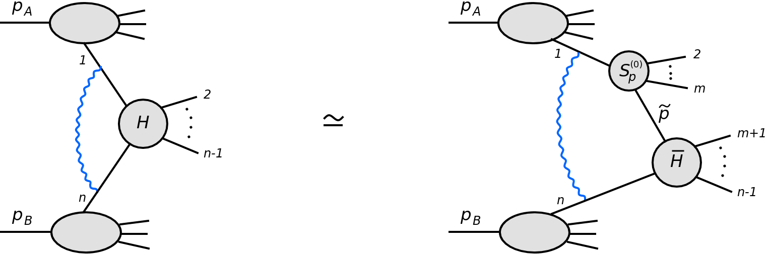
Figure 6: One loop correction to the collinear factorization at the amplitude level.

The origin of this breaking can be traced back to the Glauber/Coulomb gluons discussed earlier, hence the gluons exchanged between two incoming partons long before, or between two outgoing partons long after, the hard process. Let us consider a simplified version of Fig. 5, where we concentrate just on the amplitude (part to the left from the cut) and the only connection is that with a soft gluon between the two incoming partons. Left hand side of Fig. 6 represents the corresponding one-loop amplitude.

Let us start from a tree level version of that diagram, i.e. ignoring for a moment the gluon attached to the incoming partons $1$ and $n$. In the limit where partons $1,\ldots,m$ become collinear, the amplitude can be expressed as

$$|{\cal M}^{(0)}_{H}(1,\ldots,n)\rangle\simeq\mathbold{Sp}^{(0)}(\tilde{p},1,\ldots,m)\,|{\cal M}^{(0)}_{\bar{H}}(\tilde{p},m+1,\ldots,n)\rangle\,,$$ (3.13)

where the right hand side of the above equation corresponds to the right hand side of Fig. 6, again, ignoring the soft gluon connection. Hence, the tree level amplitude factorizes into an operator $\mathbold{Sp}^{(0)}$, which is a matrix in the colour+spin space and depends only on the collinear momenta, and the reduced amplitude $|{\cal M}^{(0)}_{\bar{H}}\rangle$, depending exclusively on the non-collinear partons.

This simple formula does not survive however at one-loop, hence the case shown in Fig. 6, as the $\mathbold{Sp}^{(1)}$ operator now has both a real and an imaginary part. The real part arises from an integration over the eikonal gluons satisfying Eq. (3.7). The imaginary part corresponds to the Glauber region of Eq. (3.8) and it is proportional to $i\,\mathbold{T}_{m+1}\cdot(\mathbold{T}_{1}-\mathbold{T}_{\tilde{p}})$, where $\mathbold{T}_{i}$ is a colour charge matrix of the particle $i$ and $\mathbold{T}_{i}\cdot\mathbold{T}_{k}\equiv\sum_{c=1}^{N_{c}^{2}-1}T_{i}^{c}T_{k}^{c}$. We see that the operator appearing in the imaginary part depends both on the collinear parton $1$, and on the non-collinear parton $m+1$. However, since the above operator is anti-Hermitian, its contributions cancel in the NLO cross sections, which involve interference terms between Born and one-loop diagrams.

The corresponding operator becomes even more complex at two loops but, also there, it can be shown that its contribution to the cross section vanishes [80, 81]. It is only at three loops where the interplay between the eikonal and the Coulomb gluons breaks the collinear factorization at the level of the cross section. Hence, the factorization breaking will have physical effects at this order, which can manifest themselves e.g. through super-leading logarithms [89, 90]. The latter appear for observables defined with non-trivial vetoes on the phase space that prevent cancellations of the Coulomb gluon contributions.

The factorization breaking effects, discussed here for the amplitudes and partonic cross sections, are expected to disappear when a sum over all diagrams is performed, as explained earlier, hence the original result of [75, 77] remains valid for inclusive observables. This can be understood in the context of the above discussion by noting that the factorization breaking terms are associated with the colour factors and those cancel each other when collisions of colourless hadrons are considered.

All order collinear factorization is a basic assumption in construction of parton showers. There, the $n$-parton cross section is computed by applying a sequence of $\mathbold{D}_{i}$ and $\mathbold{V}_{i}$ operators, which act on the $0$-parton state $|M^{(0)}\rangle$. The operators $\mathbold{D}_{i}$ correspond to real emissions and the operators $\mathbold{V}_{i}$ are the Sudakov factors that express non-emission probabilities between two momentum scales.

Hence, the Sudakov operators resum virtual and unresolved real emissions on each of the incoming or outgoing lines of the Born diagram. They do not, however, include the virtual gluon exchanges between two different external particles. Those would be exactly the Coulomb gluons depicted in Fig. 6 and would contribute at subleading colour. The study aimed at establishing whether the Coulomb gluons can be incorporated in the currently assumed, factorized structure of the parton shower algorithms has been presented in Ref. [91]. There it is found that, for the Drell-Yan process, in the first few orders of perturbation theory, the Coulomb gluons can indeed be accommodated in the probabilistic, $k_{T}$-ordered evolution algorithms. Each individual diagram involving the virtual, Coulomb-gluon exchanges and one or two real, eikonal-gluon emissions has different ordering conditions for those gluons’ transverse momenta. However, the sum of all diagrams at a given order results in the final expression in which the Coulomb gluon’s transverse momenta are always ordered with respect to the transverse momenta of the emitted (eikonal) gluons. Consequently, the factorized structure of the parton shower emissions, realized through a sequence of the $\mathbold{D}_{i}$ and $\mathbold{V}_{i}$ operators, is preserved also after the inclusion of the Coulomb gluons.

3.2 Factorization scheme

As discussed in Section 3.1.2, factorization procedure is not unique. The ambiguity seats in details of subtraction terms, as, while all the terms divergent in the collinear limit need to be subtracted from the hard part, in practice, one also subtracts a number of arbitrary finite terms. Differences between the finite terms absorbed into PDFs is what differentiates between factorization schemes.

In the context of hadron-hadron collisions, one uses almost exclusively the $\overline{\text{MS}}$ scheme [92] and all the main PDF sets [93] are indeed the $\overline{\text{MS}}$ PDFs. In the $\overline{\text{MS}}$ factorization scheme, the PDFs absorb the $1/\epsilon$ terms as well as the constant $4\pi-\gamma_{E}$. All other finite terms are left as part of the hard cross section $H$, c.f. Eq. (3.5).

However, some of the finite terms that arise from integration in $d$ dimensions originate from large distances. This happens because the $1/\epsilon$ poles are multiplied by the dimensional-regularization-specific factor $(k_{T}^{2})^{\epsilon}=(k^{2}(1-z))^{\epsilon}\simeq 1+\epsilon\ln k^{2}+\epsilon\ln(1-z)$ [94], which results in ${{\cal O}\left(\epsilon/\epsilon\right)}={{\cal O}\left(1\right)}$ contributions. The latter are not removed from the hard part by the $\overline{\text{MS}}$ subtraction scheme, though it would be more natural if they belonged to PDFs. That is the motivation behind the efforts of Refs. [95, 96, 97, 94] to come up with a factorization scheme that would better separate the short and the long distance physics.

We repeat that all factorization schemes are equivalent at a given order of perturbative expansion and the corresponding PDFs all satisfy the universality (process-independence) property. However, some finite terms may turn out to be pathological, or just inconvenient, and, therefore, switching to a different scheme can offer concrete advantages.

For example, the Monte Carlo (MC) scheme proposed in Refs. [95, 96] was motivated by construction of a matching procedure between the NLO results and the parton shower, c.f. Section 4.3.2. The latter is implemented in practice as a Monte Carlo algorithm, hence the emissions are effectively integrated in four dimensions using unitarity to cancel the soft, and in the case of the final state radiation also the collinear, divergences. Thus, if we think of the parton shower as a procedure of unfolding PDFs, then, those PDFs are definitely not of $\overline{\text{MS}}$ type but they are defined by the MC algorithm of the shower. The NLO calculations, however, are performed in $d$ dimensions and they are regularized by the $\overline{\text{MS}}$ subtraction counter-terms. Hence, they contain the finite pieces originating from the $\epsilon/\epsilon$ cancellations, like for example the term $\propto\ln(1-z)$, mentioned above.

Because of the non-compatibility of the factorization schemes used in the NLO calculations and in parton showers, NLO+PS matching faces certain non-trivial issues [98, 99]. The way out, proposed in Refs. [95, 96], is to consistently use a single factorization scheme that is compatible with the parton shower. Such a scheme is therefore called the MC factorization scheme. In the MC scheme, the $z$-dependent terms related to the $\epsilon/\epsilon$ contributions that appear in the hard part calculated in $\overline{\text{MS}}$, and come from unphysical treatment of the phase space, are absorbed into PDFs. Hence, they do not appear in the partonic cross section (3.5). On top of that, one subtracts contributions to the collinear space generated by the shower, to avoid double counting (see Refs. [95, 96] for details). With that, one defines the MC PDFs by the following shift with respect to the $\overline{\text{MS}}$ PDFs

$$f_{q(\bar{q})}^{\rm MC}(x,\mu^{2})=f_{q(\bar{q})}^{\overline{\rm MS}}(x,\mu^{2})\;+\int_{x}^{1}\frac{dz}{z}\,f_{q(\bar{q})}^{\overline{\rm MS}}\left(\frac{x}{z},\mu^{2}\right)\Delta C_{2q}(z)\;+\int_{x}^{1}\frac{dz}{z}\,f_{g}^{\overline{\rm MS}}\left(\frac{x}{z},\mu^{2}\right)\Delta C_{2g}(z)\,,$$ (3.14)

where

$$\Delta C_{2q}(z) =\frac{\alpha_{s}}{2\pi}\,C_{F}\left[\frac{1+z^{2}}{1-z}\ln\frac{(1-z)^{2}}{z}+1-z\right]_{+}\,,$$ (3.15a)

$$\Delta C_{2g}(z) =\frac{\alpha_{s}}{2\pi}\,T_{R}\,\left\{\left[z^{2}+(1-z)^{2}\right]\ln\frac{(1-z)^{2}}{z}+2z(1-z)\right\}\,.$$ (3.15b)

We recognize that the functions $\Delta C_{2q}$ and $\Delta C_{2g}$ contain the well know pieces from the $\overline{\text{MS}}$ coefficient function, c.f. Ref. [100], which in the MC scheme become parts of the MC PDFs. Since the MC scheme was defined in the context of the Drell-Yan process, whose Born level, $q{\bar{q}}\to Z$, does not involve an incoming gluon, the gluon PDF is identical to that in the $\overline{\text{MS}}$ scheme up to ${{\cal O}\left({\alpha_{s}}^{2}\right)}$ corrections. However, an extension to processes with the initial gluon, e.g. $gg\to H$, will introduce a difference between the MC and the $\overline{\text{MS}}$ schemes also for the gluon PDF.

As we see from Eq. (3.14), the change of factorization scheme can be regarded as a rotation in flavour space spanned by $(q_{i},{\bar{q}}_{i},g)$. A similar rotation, with slightly different $\Delta C$ functions, has also been used in definition of the physical scheme in Refs. [97, 94]. By removing the $\overline{\text{MS}}$ terms of $\epsilon/\epsilon$ origin, which are proportional to splitting functions, the physical scheme avoids flavour mixing. The latter is a problem of the $\overline{\text{MS}}$ scheme in which, for example, the singlet-quark distribution gets admixture of gluons. This complicates calculations of heavy quark effects [101] as well as other non-inclusive processes [94].

The differences between LO PDFs defined in the $\overline{\text{MS}}$, the MC or the physical scheme can be as large as 20% or more [96, 94]. Hence, even though formally equivalent, different choices for the factorization schemes lead to numerically non-negligible differences for predictions of physical quantities.

Related efforts to account for the logarithmically enhanced threshold contributions have been pursued in Ref. [102], where PDFs were extracted at the NLO+NLL and NNLO+NNLL accuracy. Hence, these sets are in principle the only consistent parton distributions to be used with threshold-resummed matrix elements.

3.3 TMD factorization

Collinear factorization assumes that components of the momentum of an incoming parton emitted from the hadron $A$ moving in the plus direction satisfy

$$k_{+}\gg k_{-},k_{T}\,,$$ (3.16)

hence only the $k_{+}$ component is kept while $k_{-}$ and $k_{T}$ are neglected, c.f. Eq. (3.1). This approximation is indeed valid in many situations as elaborated in the Section 3.1. However, there exist a class of observables which are directly sensitive to the transverse component of the incoming parton’s momentum.

Imagine for example measuring a distribution of the transverse momentum imbalance, $q_{T}=|p_{T1}+p_{T2}|$ between the two final state leptons in the Drell-Yan process or between two hardest jets in the hadronic production of dijets with momenta $p_{1}$ and $p_{2}$. In the limit where the two objects are oriented back-to-back in the transverse plane, $q_{T}$ is very small and its value can be comparable to the transverse momentum, $k_{T}$ of the incoming parton. In that case, neglecting $k_{T}$ will lead to a significant modification of the $q_{T}$ distribution in the low-$q_{T}$ region. In other words, observables like the $q_{T}$ spectrum or the distribution of the azimuthal distance between final state leptons or jets are directly sensitive to the transverse components of the 4-momenta of the incoming partons. Hence, the corresponding parton distribution function should depend on both $k_{+}$ and $k_{T}$. Such functions are known as transverse momentum dependent (TMD) parton distributions.

Although TMDs are not the main focus of this review, we note in passing that determination and modeling of the transverse momentum dependent distributions is an active domain of research. One of the classic approaches is due to Collins, Soper and Sterman (CSS) [103], where TMDs are expressed in terms of the collinear PDFs convoluted with functions which resum the transverse emissions in coordinate space. For more details on evolutions, properties and parametrizations of TMDs see Ref. [78] as well as the recent reviews  [104, 105]. In order to facilitate usage and comparison between different fits and parametrizations of TMDs, the project called TMDlib (and a related TMDplotter) [106] has been started. It provides a common interface to a wide range of distributions allowing for convenient phenomenology studies.

Understandably, TMDs call for an extension of the collinear factorization formula to the transverse momentum dependent factorization. As we shell see, this poses serious challenges and many questions are still unanswered. The remaining part of this section aims at summarizing the status of the TMD factorization across various processes, with special emphasis on jet production, and recent progress in that domain.

Transverse gauge links and non-universality of TMDs

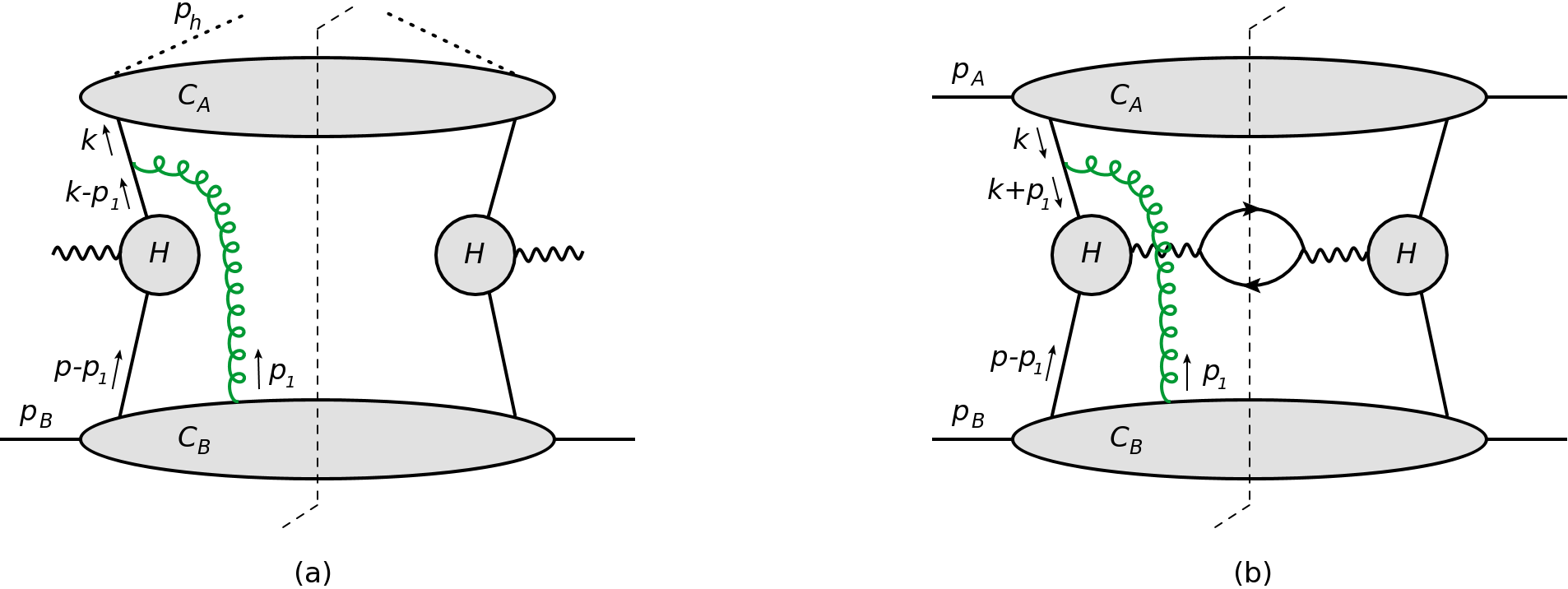
Figure 7: Single gluon exchange in SIDIS (a) and DY (b).

Let us consider a single-gluon exchange in the following two processes: semi-inclusive deep inelastic scattering (SIDIS), shown in Fig. 7 (a) and Drell-Yan (DY), depicted in Fig. 7 (b). The figures introduce necessary notation and it is understood that $p^{-}=p_{1}^{-}=k^{+}=0$, hence $k^{-}\approx q^{-}=Q/\sqrt{2}$, where $q$ is the 4-momentum of the vector boson, while $Q$ denotes its virtuality.

The SIDIS diagram involves the following propagator [107]

$$\frac{\not{k}-\not{p}_{1}+m}{(k-p_{1})^{2}-m^{2}+i\epsilon}\approx\frac{(\not{k}+m)-\not{n}_{+}\,p_{1}^{+}-\not{p}_{1T}}{-p_{1}^{+}\,Q\sqrt{2}+(k_{T}-p_{1T})^{2}-m^{2}+i\epsilon}\,,$$ (3.17)

while, for DY, we have

$$\frac{-\not{k}-\not{p}_{1}+m}{(k+p_{1})^{2}-m^{2}+i\epsilon}\approx\frac{-(\not{k}-m)-\not{n}_{+}\,p_{1}^{+}-\not{p}_{1T}}{p_{1}^{+}\,Q\sqrt{2}+(k_{T}+p_{1T})^{2}-m^{2}+i\epsilon}\,,$$ (3.18)

where $m$ is a quark mass and $n_{\pm}$ are the light-like vectors satisfying $n_{+}\cdot n_{-}=1$.

The first thing we notice is that the two expressions have different signs in front of $p_{1}^{+}\,Q\sqrt{2}$ in the denominators. This comes from different directions of the quark with momentum $k$ in Fig. 7. In the case of SIDIS, the gluon connects the collinear subgraph $C_{B}$ with the outgoing quark, whereas in DY, the gluon is attached to the incoming quark.

As is evident from Fig. 7, the gluons connecting the hard and the collinear parts break topological factorization graph by graph. It turns out however that when the graphs are summed up for each process, one is able to apply the Ward identities and consequently factor out all the gluon connections into Wilson lines and include them in definitions of TMDs [77], very much like in the case of collinear factorization discussed earlier. There are however subtle differences.

The diagrams in Fig. 7 and the expressions in Eqs. (3.17) and (3.18) correspond to the first terms in the expansion of the Wilson line (3.11) for SIDIS and DY, with $n^{\mu}\sim k^{-}\sim q^{-}=Q/\sqrt{s}$. The term $p_{1}^{+}\,Q\sqrt{2}$ originates from eikonal vertex $\sim n\cdot p_{1}$ (see [77] for details on eikonal Feynman rules). Because of the sign difference in the $p_{1}^{+}\,Q\sqrt{2}$ term, the gauge links resulting from summation of multi-gluon exchanges will go along different paths for the two processes. Therefore, the factorization formula for SIDIS and DY will include different transverse momentum dependent parton distribution functions. This difference disappears after integration over the transverse momentum [75, 76, 108, 109, 110], however, at the level of the unintegrated TMDs, the strict universality of parton distributions is lost.

Thus, we have discovered a very important feature of QCD factorization: the parton distribution functions are universal at the level of the integral (collinear PDFs) but not necessarily at the level of the integrand (TMDs) [111].

The second subtlety concerning TMD factorization is related to the last term in Eqs. (3.17) and (3.18), which is proportional to the transverse component of gluon’s momentum $p_{T1}$. As observed in Refs. [112, 107], this term will yield leading twist contributions in the transverse direction which in general survive at the light-cone infinity. More specifically, those contributions do not appear in covariant gauges but they are non-vanishing for the light-cone gauges. Hence, unlike in the case of the collinear factorization, here, the transverse components of the gauge links will not vanish.

Altogether, the gauge-invariant TMDs are defined as

$$f(\xi,k_{T})=\int\frac{dw^{-}d^{2}\mathbold{w}_{T}}{(2\pi)^{3}}e^{-i\xi P^{+}w^{-}+i\mathbold{k}_{T}\cdot\mathbold{w}_{T}}\langle P|\phi^{\dagger}(0,0,0)\,{\cal U}^{[{\cal C}]}(0,w^{-},\mathbold{w}_{T})\,\phi(0,w^{-},\mathbold{w}_{T})|P\rangle\,,$$ (3.19)

where, this time, in order to assure gauge invariance, the object ${\cal U}^{[{\cal C}]}(0,w^{-},\mathbold{w}_{T})$ is a gauge link, which is in general composed of multiple Wilson lines in both the light-cone and the transverse directions

$${\cal W}^{n}_{[a,b]}={\cal P}\exp\left[-ig\int_{a}^{b}dz\,n\cdot A(z)\right]\,,\qquad\qquad{\cal W}^{T}_{[a,b]}={\cal P}\exp\left[-ig\int_{a}^{b}dz_{T}\cdot A_{T}(z)\right]\,.$$ (3.20)

In particular, for SIDIS, one has to use the gauge link ${\cal U}^{[+]}$ involving future-pointing Wilson lines, wheres for DY, gauge invariance of the TMD is achieved with the link ${\cal U}^{[-]}$, which involves past-pointing Wilson lines. The above gauge links for SIDIS and DY are defined as

$${\cal U}^{[\pm]}={\cal W}_{[(0^{-},\mathbf{0}_{T});(\pm\infty^{-},\mathbf{0}_{T})]}^{n}{\cal W}_{[(\pm\infty^{-},\mathbf{0}_{T});(\pm\infty^{-},\mathbold\mathbold{w}_{T})]}^{T}{\cal W}_{[(\pm\infty^{-},\mathbold\mathbold{w}_{T});(w_{-},\mathbold\mathbold{w}_{T})]}^{n}\,,$$ (3.21)

and the corresponding paths are depicted in Fig. 8.

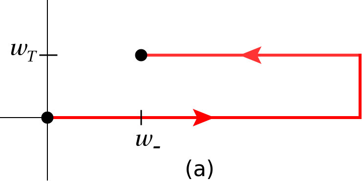
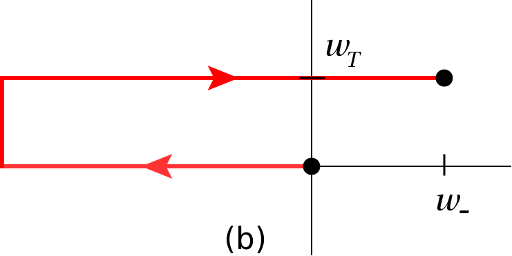
Figure 8: The gauge-link structure in the correlator $\Phi$ in (a) SIDIS: $\mathcal{U}^{[+]}$ and (b) DY: $\mathcal{U}^{[-]}$.

Hence, we have two different types of TMDs for SIDIS and DY and the strict factorization property is lost due to the loss of universality of the TMDs. However, it turns out that the SIDIS and DY TMDs are related by time-reversal and differ only by the sign flip for two of the TMDs [113], the so-called Sivers function [114] and the Boer-Mulders function [115]. Hence, the loss of strict universality does not spoil predictive power.

It is important to notice that the non-equality of TMDs in SIDIS and DY comes from the differences in the colour flow, c.f. Fig. 7. The colour running via an outgoing quark in SIDIS results in future pointing Wilson line and the colour flowing via an incoming quark in DY leads to past pointing Wilson line.

For the $k_{T}$-integrated cross sections, the transverse link does not affect the result and one gets ${\cal U}^{[+]}$ = ${\cal U}^{[-]}={\cal W}_{[0,w^{-}]}$ [107]. This can be seen directly in Eq. (3.19). Integration over $\mathbold{k}_{T}$ produces delta function $\delta^{(2)}(\mathbold{w}_{T})$, which fixes the transverse gauge link at ${\cal W}_{[(0;\mathbf{0}_{T});(0;\mathbf{0}_{T})]}^{T}=1$. As can be seen in Fig. 8, without the transverse separation, the gauge links ${\cal U}^{[+]}$ and ${\cal U}^{[-]}$ both reduce to ${\cal W}_{[0,w^{-}]}$.

However, in order to achieve full gauge invariance of the transverse momentum dependent gluons, one has to include also transverse gauge links, even at leading twist [112, 107]. Without them certain distributions, referred to as $T$-odd functions [114, 116, 115], would be zero [107]. The need for the transverse gauge links, connecting the light-cone gauge-links at infinity, is visible most notably the light-cone gauges which introduce additional singularities [112] leading to non-vanishing transverse components at light-cone infinity. Those modes can be though of as zero-light-cone-momentum, transverse gluons. Hence, as opposed to the collinear factorization, the TMD factorization requires in general contributions from transverse-gluon connections between the hadron and the hard part, which are resummed into transverse Wilson lines.

Dijet production

The non-universality of the transverse momentum dependent parton distributions between SIDIS and DY is a minor problem as it reduces to a sign difference. The situation becomes much more complicated for processes with two incoming and two outgoing partons, as for example dijet production in hadron-hadron collisions. Here, the longitudinal (and at the light-cone infinity, also the transverse) gluons connect both to the partons in the initial and in the final state. As found in Refs. [117, 118], eikonalization of those gluons is possible (at least to the order $g$) for an arbitrary hard process, but the procedure leads to appearance of new gauge link structures, like for example

$${\cal U}^{\left[\square\right]}=\mathcal{U}^{\left[+\right]}\mathcal{U}^{\left[-\right]\dagger}=\mathcal{U}^{\left[-\right]}\mathcal{U}^{\left[+\right]\dagger}\,.$$ (3.22)

As a consequence, dijet production in hadronic collisions requires new types of TMDs, which are not reducible to those encountered in SIDIS or DY. As we shall see, the differences appear even between different channels in dijet production, hence not only that the TMDs are not universal but the cross section for dijet production does not factorize in the strong sense. We shall now discuss this question in more detail.

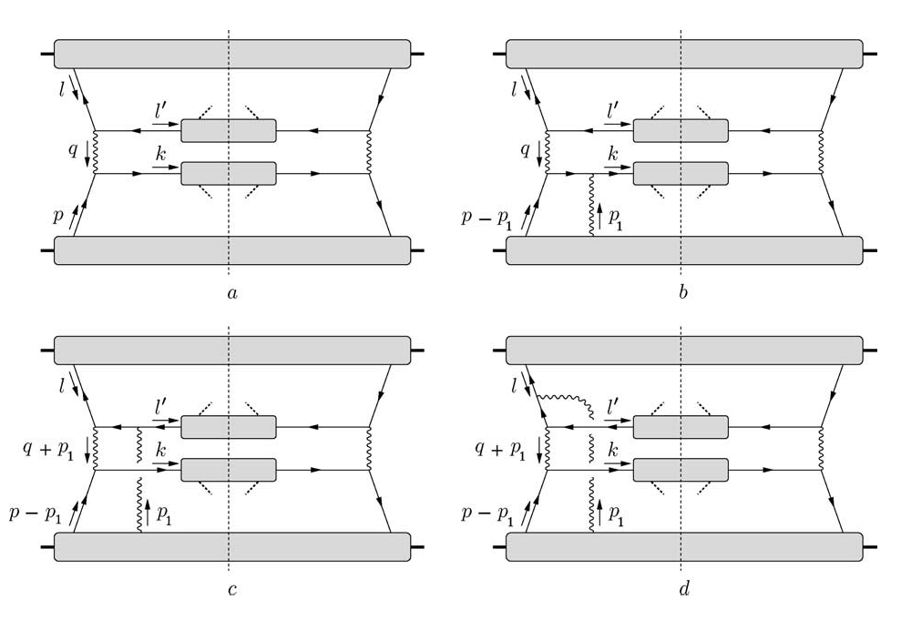
Figure 9: Insertions of longitudinal gluons for $q{\bar{q}}\to q{\bar{q}}$ process. Figure from Ref. [117].

In order to construct the gauge links for a process involving two incoming and two outgoing partons, one needs to consider all gluon attachments between the hadron and the hard part of the diagram. Fig. 9 shows an example for the $q{\bar{q}}\to q{\bar{q}}$ process, where diagram (a) is a tree level contribution, diagrams (b) and (c) correspond to attaching the gluon to the final-state partons, and, in diagram (d), the gluon is attached to the initial-state parton. The result for the cross section comes from the sum of diagrams of Fig. 9 (a)-(d) and reads [117]

$$\sigma \propto \int\mathrm{d}^{4}p\,\mathrm{d}^{4}k\,\mathrm{d}^{4}l\,\mathrm{d}^{4}l^{\prime}\ \delta^{4}(p+q-k)\ \Big{(}\frac{1}{q^{2}}\Big{)}^{2}\ \bigg{\{}\text{Tr}\big{[}\Phi(p)\gamma^{\mu}\Delta(k)\gamma^{\nu}\big{]}\text{Tr}\big{[}\,\overline{\Phi}(l)\gamma_{\nu}\overline{\Delta}(l^{\prime})\gamma_{\mu}\big{]}$$ (3.23)

$$\ -g_{2}\int\mathrm{d}^{4}p_{1}\frac{1}{-p_{1}^{+}+i\epsilon}\text{Tr}\big{[}\Phi_{A}^{\alpha}(p,p-p_{1})\gamma^{\mu}\Delta(k)\gamma^{\nu}\big{]}\text{Tr}\big{[}\,\overline{\Phi}(l)\gamma_{\nu}\overline{\Delta}(l^{\prime})\gamma_{\mu}\big{]}$$

$$\ +g_{1}\int\mathrm{d}^{4}p_{1}\frac{1}{-p_{1}^{+}+i\epsilon}\text{Tr}\big{[}\Phi_{A}^{\alpha}(p,p-p_{1})\gamma^{\mu}\Delta(k)\gamma^{\nu}\big{]}\text{Tr}\big{[}\,\overline{\Phi}(l)\gamma_{\nu}\overline{\Delta}(l^{\prime})\gamma_{\mu}\big{]}$$

$$\ +g_{1}\int\mathrm{d}^{4}p_{1}\frac{1}{p_{1}^{+}+i\epsilon}\text{Tr}\big{[}\Phi_{A}^{\alpha}(p,p-p_{1})\gamma^{\mu}\Delta(k)\gamma^{\nu}\big{]}\text{Tr}\big{[}\,\overline{\Phi}(l)\gamma_{\nu}\overline{\Delta}(l^{\prime})\gamma_{\mu}\big{]}\,\bigg{\}}\,,$$

where the couplings $g_{1}$ and $g_{2}$ were introduced to distinguish between the connections to the final and to the initial state particles, respectively. The transition: hadron $\to$ quark is described by the correlator $\Phi(p)$, while the transition: hadron $\to$ quark + gluon by $\Phi^{\alpha}_{A}(p,p-p_{1})$. The functions $\Delta(k)$ and $\Delta(l^{\prime})$ represent quark $\to$ hadron transitions, hence these are fragmentation functions.

The three ${{\cal O}\left(g\right)}$ terms in Eq. (3.23) correspond to the first terms in the expansion of the gauge links $U_{g_{2}}(\infty^{-},\mathbold{w}_{T};w^{-},\mathbold{w}_{T})$, $U_{g_{1}}(w^{-},\mathbold{w}_{T};\infty^{-},\mathbold{w}_{T})$, and $U_{g_{1}}(-\infty^{-},\mathbold{w}_{T};w^{-},\mathbold{w}_{T})$, respectively. Hence, at least to the order $g$, it is possible to account for the gluon connections by reweighting the non-local bi-products of operators, which define the TMDs, by the gauge links, as in Eq. (3.19). The above implies that, even in the complex processes like the dijet production, it is possible to define TMDs in a gauge invariant manner.

As shown in Ref. [118], similar procedure can applied to subprocesses with gluons. The resulting TMDs involve all types of gauge links, ${\cal U}^{\left[+\right]}$, ${\cal U}^{\left[-\right]}$ and ${\cal U}^{\left[\square\right]}$, multiplying each other and combined with several different colour factors. The complete set of definitions of the TMDs appearing in the dijet process can be found in Ref. [118].

We see that the dijet production in hadronic collisions requires very complicated, subprocess-dependent TMDs. Hence, the strict factorization property does not hold. It survives however in a generalized form since the differential cross section for the process of hadroproduction of two coloured partons, $h_{1}+h_{2}\mapsto a+b\to c+d$ can be written as

$$d\sigma=\sum_{i}\mathcal{F}_{a/h_{1}}^{(i)}(x_{1},k_{T})\otimes\mathcal{F}_{b/h_{2}}^{(i)}(x_{2},k_{T})\otimes H_{ab\to cd}^{(i)}\,.$$ (3.24)

In the above, $h_{1}$ and $h_{2}$ denote the incoming hadrons. Each of them provides a QCD parton, here, respectively $a$ and $b$. $\mathcal{F}_{p/h}^{(i)}$ is a TMD of $i$-th type involving the parton $p$ and the hadron $h$. Those TMDs are convoluted with the hard factors $H_{ab\to cd}^{(i)}$, where $c$ and $d$ correspond to the outgoing partons. The hard factors are gauge invariant combinations of the cut diagrams contributing in a given channel, as explained in Refs. [119, 120]. Each term of the above sum has the same form as the strict factorization formula. However, the gauge links appearing in the generalized TMDs, $\mathcal{F}_{p/h}^{(i)}$, depend on the hard subprocess.

Let us stress that we have deduced Eq. (3.24) based on the complete analysis with just a single gluon attachment, following Refs. [117, 118]. Partial contributions from two-gluon attachments have also been studied [118] but, for now, it is only a conjecture that Eq. (3.24) will hold at higher orders.

Differences in the link structures and the resulting process dependence can be understood by looking again at Fig. 9. As discussed earlier, the gluons connecting TMDs with the hard part can be absorbed into a given quark or gluon correlator. This achieves two goals: it renders the correlator gauge invariant and it allows one to factorize it from the rest of the diagram.

However, this procedure requires pulling the gluons through the hard part, which can be done using colour flow identities like Fierz identity. The hard part, in general, has a non-trivial colour structure. Hence, the result of this procedure depends on the type of partons participating in the hard scattering, as well as whether the gluon which is pulled through the hard part was attached to the initial or to the final state parton. The situation is particularly complex for diagrams involving the $gg\to gg$ hard process, where six different colour structures appear in the cut diagrams (see Refs. [118, 120] for details). It is quite clear that the procedure of pulling the gluons into the correlator introduces dependence on the sub-process and, as a consequence, leads to process-dependence of the resulting TMDs. Similar problems occur in proofs of the collinear factorization but, there, the differences amongst the gauge links cancel between graphs after integration over the transverse momentum [110].

Construction of the gauge links necessary for gauge invariant definitions of process-dependent TMDs, which allowed for a conjecture of Eq. (3.24) has been performed with up to two longitudinal gluon attachments (thus up to the order $g^{2}$ in expansion of the gauge links) [117, 118]. What is more important however, is that the two gluons were always taken from the same hadron. This, in general, is not enough for QCD in processes involving four hadrons. Indeed, as shown in Ref. [121], even the generalized factorization of Eq. (3.24) breaks down in QCD at the level of two gluons. The terms responsible for this effect correspond to diagrams in which each of the two gluons is attached to different hadron.

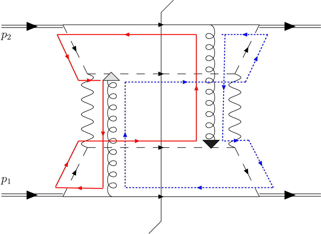
Figure 10: Example of a graph contribution to violation of generalized TMD factorization in a non-Abelian theory. The red an the blue lines illustrate colour flow. Figure from Ref. [121].

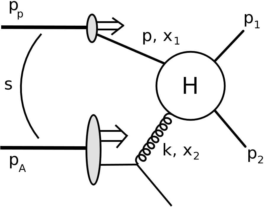
Figure 11: Inclusive dijet production in p+A collision. $H$ represents hard scattering. The solid lines coming out of $H$ can be either quarks or gluons. Figure from Ref. [120].

Ref. [121] verifies the assumption of the generalized TMD factorization by finding an explicit counter-example, in which Eq. (3.24) is not valid for the double spin asymmetry (DSA) in a non-Abelian theory. In order to facilitate the proof, Ref. [121] uses a simplified model, where the complicated structure of multiple sub-processes and colour flows of QCD is reduced to just a single sub-process with one colour flow. The particle content of the model is shown in Fig. 11. It consists of the incoming Dirac fields, neutral under the $SU(N_{c})$ gauge group (double line), spectator diquark (solid line), active, scalar “quark” (dashed line), the gluon (curly line) and a massive, colour-neutral boson (wavy line) exchanged in the hard interaction. The latter allows for great simplification of the colour flow in the hard process as compared to the standard QCD. In fact, as seen in Fig. 11, the colour (denoted by red and blue lines) is not exchanged in the hard process but only through eikonal gluons.

As discussed earlier, the standard TMD factorization is violated in QCD at the level of one gluon. In the simplified non-Abelian theory [121], similar breaking arises at the level of two gluons when both connect the same hadron to a parton on the opposite side of the hard process. These diagrams cannot be absorbed into standard Wilson lines. Hence, new types of gauge links need to be introduced, which results in non-universality of the TMDs.

At the level of two gluons there are however other diagrams, which are not included even in the modified Wilson lines. These are the two-gluon diagrams with one gluon radiated from each hadron attaching to the parton on the opposite side of the hard process. An example of such diagram is shown in Fig. 11.

The reason why the diagram of Fig. 11 cannot be absorbed by the modified Wilson line is that the latter includes a trace over colour, hence, its ${{\cal O}\left(g\right)}$ expansion is proportional $\text{Tr}[t^{a}]=0$. Therefore, the diagram shown in Fig. 11 cannot be generated by a Wilson loop expansion, yet it turns out to be non-zero because of a non-trivial colour flow, impossible to accommodate by a product of ${{\cal O}\left(g\right)}$ terms from two Wilson lines. The diagram of Fig. 11 requires exchanges of non-singlet gluons. However, due to the condition $\text{Tr}[t^{a}]=0$, only colour singlet gluon can be exchanged between a spectator and the Wilson loop at the single-gluon level. Therefore, we are left with a diagram that goes beyond what can be generated by the Wilson lines and the factorization is broken.

The above direct counter-example, found for the double spin asymmetry observable, shows that the general proof of TMD factorization does not exist in a simplified model. Similar breaking is expected to happen also for unpolarized cross sections in real QCD at the level of three gluon exchanges (a diagram similar to Fig. 11 with an extra copy of the gluon on one side of the cut) [121] .

3.4 Factorization in forward jet production

We have seen that the general formula for the TMD factorization for the dijet process is complex and its theoretical status is a subject of current debate. In this section, we shall discuss a special sub-class of dijet processes in which both jets are produced at large rapidities. This case corresponds to an asymmetric situation, in which the two colliding objects are probed in very different momentum ranges.

The process is shown schematically in Fig. 11. The fractions of the longitudinal momenta of the incoming parton from the projectile, $x_{1}$, and from the target, $x_{2}$, can be expressed in terms of the rapidities and the transverse momenta of the produced jets as

$$x_{1}=\frac{1}{\sqrt{s}}\left(p_{T1}e^{y_{1}}+p_{T2}e^{y_{2}}\right)\,,\quad\quad x_{2}=\frac{1}{\sqrt{s}}\left(p_{T1}e^{-y_{1}}+p_{T2}e^{-y_{2}}\right)\,.$$ (3.25)

In the limit $y_{1},y_{2}\gg 0$, we have: $x_{1}\sim 1$ and $x_{2}\ll 1$. As we know, the number of gluons grows quickly with decreasing momentum fraction. Therefore, the forward dijet production corresponds to dilute-dense collisions, where the projectile, probed at a high momentum fraction, hence appearing as dilute, can be described in terms of a collinear parton distribution. On the other hand, one has to use an unintegrated parton distribution on the dense target side, as the latter, probed at low $x$, will have much bigger fraction of partons with high transverse momenta. Since those partons will be mostly gluons, we limit our discussion to subprocesses in which the parton from the target is always an off-shell (meaning $k^{2}\neq 0$) gluon, as illustrated in Fig. 11.

3.4.1 Generalized TMD factorization for forward jets

Ref. [119] exploited the results of Ref. [118] to derive the exact form of the effective TMD factorization, given schematically in Eq. (3.24), for a range of processes studied in the small-$x$ limit. In the case of dijet production in dilute-dense, hadron-hadron collisions, one obtains

$$\frac{d\sigma^{pA\rightarrow{\rm dijets}+X}}{dy_{1}dy_{2}d^{2}p_{T1}d^{2}p_{T2}}=\frac{\alpha_{s}^{2}}{(x_{1}x_{2}s)^{2}}\sum_{a,c,d}x_{1}f_{a/p}(x_{1},\mu^{2})\sum_{i}H_{ag\to cd}^{(i)}\mathcal{F}_{ag}^{(i)}(x_{2},k_{T})\frac{1}{1+\delta_{cd}}\,,$$ (3.26)

where the notation is similar to that of Eq. (3.24), but, now, the incoming parton $b$ is always a gluon, $g$, and it comes from the dense object $A$, while the parton from the dilute initial hadron, $p$, denoted as $a$, can be either a (anti-)quark or a gluon. The factor $1/(1+\delta_{cd})$ is a symmetry factor needed in the case the $gg$ final state. (This factor is not explicit in Eq. (3.24) as the latter is only schematic.)

As found in Ref. [119], the above, most complicated case involves eight different gluon TMDs, which in the limit of large $N_{c}$ reduce to five that can be written down as convolutions of two fundamental distributions: the so-called dipole distribution and the Weizäsacker-Williams distribution (WW). We recall that the dipole distribution enters directly into various inclusive observables like the structure function in DIS, total cross section in DY and SIDIS, as well as hadron production in DIS and $pA$ collisions and photon-jet production in $pA$. None of the above involves the WW gluon. The latter can be however determined from dijets production in DIS, as it is the only distribution appearing in that process. Finally, dijets production in $pA$ involves both the dipole and the Weizäsacker-Williams gluon. Though appearing in factorization formulae for many processes, the dipole distribution does not have a clear partonic interpretation. On the other hand, the WW distribution corresponds to the number density of gluons, in the light-cone gauge, inside a hadron.

All the accompanying hard factors, $H_{ag\to cd}^{(i)}$, appearing in Eq. (3.26), have been also calculated in the limit of large $N_{c}$ and ignoring the transverse momentum dependence (hence taking $k_{T}=0$) [119]. This last approximation restricted the result to the case $p_{T1},p_{T2}\gg k_{T}\sim Q_{s}$, which, following the relation

$$k_{T}^{2}=|\mathbold{p_{T1}}+\mathbold{p_{T2}}|^{2}=p_{T2}^{2}+p_{T2}^{2}+2p_{T1}p_{T2}\cos\Delta\phi\,,$$ (3.27)

corresponds to the production of two jets which are nearly back-to-back in the transverse plane. The $Q_{s}$ above denotes the saturation scale, i.e. a momentum scale below which non-linear effects become very relevant. Its typical value is estimated at around a few GeV, depending on $x$, as well as the number of nucleons in the target.

It was also found in Ref. [119] that the same factorization formula, Eq. (3.26), involving identical gluon distributions, can be derived from the colour glass condensate formalism (CGC) [17] in the correlation limit (i.e. for nearly back-to-back dijet configurations). In CGC, the gluons inside a dense, colour-neutral object are treated semi-classically, which is justified at high densities. This leads to an effective theory with colour sources, $\rho$, forming the static and large-$x$, and the gauge fields, forming the dynamical and small-$x$, degrees of freedom. Then, renormalization group equation is used for evolution of the sources in $x$. The distribution of the sources, $W[\rho]$, describes properties of saturated gluons at small $x$. Given the differences between the standard QCD framework and that of CGC, the fact that the two lead to identical results (in the correlation limit) should be regarded as a highly non-trivial check of the generalized TMD factorization formula of Eq. 3.26.

We note that, since Ref. [119] relies on gauge link classification obtained rigorously at the level of a single-gluon exchange  [118], it may in principle suffer from the same issues that were raised in Ref. [121] and discussed above in Section 3.3. Hence, the all-order validity of the generalized TMD factorization formula of Eq. (3.26) still needs to be demonstrated. What is special about the dilute-dense limit is the fact that one of the incoming hadrons, which we call a projectile, is described with an integrated parton distribution. This opens a possibility that the TMD-factorization-breaking contributions, like the one illustrated in Fig. 11, will cancel after integration, just like they do in the case of the collinear factorization. However, rigorous study is still needed to settle this point.

3.4.2 High energy factorization

We note that the production of a dijet system moving in the forward direction is a multi-scale problem. The highest scale is the collision energy $\sqrt{s}$, then the jets’ transverse momenta $p_{T1},p_{T2}$ and, finally, the dijet imbalance (or equivalently, the transverse momentum of the off-shell gluon). As we see in Eq. (3.27), this last scale can in principle be anywhere below the transverse momenta of the individual jets. The case with $k_{T}\sim p_{T1},p_{T2}$, corresponds to a very small angle, $\Delta\phi$, between the two forward jets, while if $k_{T}\ll p_{T1},p_{T2}$, the two jets are almost back-to-back. The latter is the domain of application of the generalized (effective) TMD factorization, just discussed in Section 3.4.1. In the former case, however, another type of factorization emerges. This is the so-called high energy factorization (HEF), often also referred to as the $k_{T}$ factorization.

The high energy factorization has been proposed in the context of heavy quark production [122, 123] (which is a multi-scale problem as well, with the mass of a heavy quark playing a role similar to jet’s transverse momentum in the case discussed here).

The key observation is that, at high energies, the dominant contribution to the cross section comes from exchanges of longitudinal gluons, whereas other terms are sub-dominant. Hence, the cross section formula can be factorized into an unintegrated parton distribution function (TMD), which emits an off-shell (i.e. $k_{T}\neq 0$) gluon, and an off-shell matrix element. Ref. [123] derives an effective procedure which guarantees gauge invariance of the off-shell amplitudes within a subclass of axial gauges (see also Ref. [120] for details). Recently, fully general methods for calculating the off-shell amplitudes, which can be used in the framework of the high energy factorization, have been developed [124, 125].

In the context of the forward dijet production, the HEF formula takes again a hybrid form, as we only need to consider the off-shell gluon effects in one of the colliding hadrons [126, 127]

$$\frac{d\sigma^{pA\rightarrow{\rm dijets}+X}}{dy_{1}dy_{2}d^{2}p_{T1}d^{2}p_{T2}}=\frac{1}{16\pi^{3}(x_{1}x_{2}s)^{2}}\sum_{a,c,d}x_{1}f_{a/p}(x_{1},\mu^{2})\,|\overline{{\cal M}_{ag^{*}\to cd}}|^{2}{\cal F}_{g/A}(x_{2},k_{T})\frac{1}{1+\delta_{cd}}\,.$$ (3.28)

Note that the above cross section needs only a single TMD, in contrast to the effective TMD factorization discussed earlier. The ${\cal F}_{g/A}$ parton distribution is the dipole distribution, usually determined from fits to DIS data. Another difference with respect to Eq. (3.26) is that, here, the hard factor (which, because we have only one TMD, is just a matrix element squared) depends on the transverse momentum, hence, we shall refer to it as an off-shell matrix element. The complete set of the off-shell matrix elements needed for hadroproduction of forward jets were calculated and analyzed in Refs. [126, 128]. We shall further elaborate on the relation between Eqs. (3.26) and (3.28) in the following subsection.

As demonstrated in Ref. [120], the factorization formula (3.28) can be also derived for all channels from the CGC approach in the kinematic window $p_{T1},p_{T2}\sim k_{T}\gg Q_{s}$. This limit corresponds to the dilute target approximation, hence, it should not be employed to study non-linear effects in dense systems. It can however be used in the, so-called, geometric scaling region, where the linear approximation is still valid but saturation effects can be felt [127, 129, 130]. However, the HEF formula is not applicable in situations corresponding to $k_{T}\sim Q_{s}$. This deficiency is fixed by the improved TMD factorization framework, which we discuss next.

3.4.3 Improved TMD factorization

A framework unifying the HEF formalism (applicable when $k_{T}\sim p_{T1},p_{T2}$) and the generalized TMD formalism (applicable for $k_{T}\ll p_{T1},p_{T2}$) was proposed in Ref. [120]. It can be regarded as a generalization of Ref. [119] to the case in which the $k_{T}$ dependence is kept also in the hard factors. The latter were computed with two independent methods: the original procedure of Refs. [122, 123] as well as the colour ordered amplitudes approach [131]. The improved factorization formula reads

$$\frac{d\sigma^{pA\rightarrow{\rm dijets}+X}}{d^{2}P_{t}d^{2}k_{t}dy_{1}dy_{2}}=\frac{\alpha_{s}^{2}}{(x_{1}x_{2}s)^{2}}\sum_{a,c,d}x_{1}f_{a/p}(x_{1},\mu^{2})\sum_{i=1}^{2}K_{ag^{*}\to cd}^{(i)}\Phi_{ag\rightarrow cd}^{(i)}(x_{2},k_{T})\ \frac{1}{1+\delta_{cd}}\ ,$$ (3.29)

where $K_{ag^{*}\to cd}^{(i)}$ and $\Phi_{ag\rightarrow cd}^{(i)}$ are the new hard factors and the new TMDs, replacing, respectively, $H_{ag\to cd}^{(i)}$ and $\mathcal{F}_{ag}^{(i)}$ from Eq. (3.26). As we see, $K_{ag^{*}\to cd}^{(i)}$ is a hard factor for an off-shell, hence $k_{T}$-dependent, incoming gluon. We also note that the new formula has two TMDs per each channel, thus, six altogether. This is fewer than the eight TMDs appearing in Eq. (3.26). The reason is that the generalized TMD factorization formula (3.26) was found to have some redundancy, which has been removed in Eq. (3.29). That is most readily seen in the colour ordered amplitude formalism. The last improvement of Ref. [120] was a restoration of the full $N_{c}$ dependence in the hard factors. We refer to the original article for explicit expressions for the new hard factors and TMDs.

The improved TMD factorization (3.29) is valid in the limit $p_{T1},p_{T2}\gg Q_{s}$ for an arbitrary value of $k_{T}$, hence it provides a robust framework for studies of the non-linear domain of QCD with hard jets. Preliminary results indicate differences with respect to the HEF formalism [132] but the full potential of this new framework for phenomenology of forward jet production is yet to be explored.

We note that theoretical status of the improved TMD factorization formula is similar to that of the generalized TMD factorization discussed in Section. 3.4.1. In particular, it remains to be shown that large logarithms generated by higher order corrections can be absorbed into TMDs and the remaining, factorization-breaking, contributions vanish. As explained in Section 3.3, TMD factorization for dijet production appears to be broken, even in its generalized form. What is special about the case considered here is that, in the formula (3.29), only one hadron is described by the TMDs. The other incoming hadron is taken in the collinear approximation and, because we discuss jet production, the outgoing partons do not involve fragmentation functions.

We emphasize that Eq. (3.29) has limits, which are solid results of QCD. In the case $k_{T}\ll p_{T1},p_{T2}$, the $k_{T}$ dependence can be neglected in the hard factors. Then, when Eq. (3.29) is integrated over $k_{T}$, one effectively integrates only the TMDs, which, by the same principle as discussed for SIDIS and DY in Section 3.3, will all (except one, which vanishes) turn into a single, integrated PDF and the standard collinear factorization formula is recovered. On the opposite end, when $k_{T}\lesssim p_{T1},p_{T2}$, the transverse part of the Fourier transform of Eq. (3.19) becomes quickly varied and the $\mathbold{w}_{T}$ dependence of the gauge links can be neglected. Then, again, all the gauge links become identical and all the six $\Phi_{ag\rightarrow cd}^{(i)}$ TMDs collapse to a single function, which can be identified with $\mathcal{F}_{g/A}$. Hence the HEF factorization (3.28) is recovered as it should be.

4 Jet production in hadron-hadron collisions

After having discussed the definitions and properties of jets and the subtelties related to QCD factorization, in this section, we turn to jet production processes at hadron colliders. Aiming at precise QCD predictions, we shall first discuss potential limiting factors, such as non-perturbative effects and dependence of the results on jet definition choices. Then, we will turn to the state-of-the-art perturbative calculations for processes involving jets and show selected comparisons to the LHC data. Finally, we shall devote separate subsections to the questions of vetoing jets and to the forward jet production.

4.1 Nonperturbative effects

Although jets can be, to a first approximation, regarded as the objects that point to the partons undergoing a hard scattering, the exact relation between partons and jets is significantly more complex. One type of corrections to this simple picture comes from higher order terms of the perturbative series, as each quark or gluon leaving the hard scattering can dress into real and virtual partons. The other type of correction is related to the partons $\to$ hadrons transition, which has to happen at some low scale before jets are registered in the detector. This hadronization effects are of genuinely non-perturbative nature. A third type of corrections to the partons $\leftrightarrow$ jets relation is specific to hadron colliders and it arises from interactions between hadron remnants or between other hadrons from the same bunches that cross during the collision. Those result in additional radiation that is likely to contaminate the jets initiated by the hard partons, thus obscuring the relation between the two. Such radiation, called the underlying event and pileup has mixed, perturbative and non-perturbative nature. We start our discussion from the corrections with non-perturbative components, while in the following sections, we shall turn to the effects arising due to higher order perturbative radiation.

4.1.1 Underlying event and pileup

As mentioned above, a hard jet in hadron-hadron collision is always produced on top of a pedestal formed by the soft and semi-hard particles, referred to as the underlying event (UE). The underlying event, although consisting mostly of soft particles, is different than the activity measured without a jet trigger, the so-called minimum bias (MB). In particular, the overall transverse momentum accumulated in UE will depend on the $p_{T}$ of the produced jets, as well as on the azimuthal distance to the jet.

On top of the UE activity, each measurement at the LHC faces the problem of pileup (PU), that is the radiation coming from independent hadron-hadron collisions occurring in the same bunch crossing. Typical numbers of such crossing varies between $10-100$ in the LHC environment. Because pileup comes from incoherent proton-proton collisions, unlike UE, it is expected to be independent of jet activity.

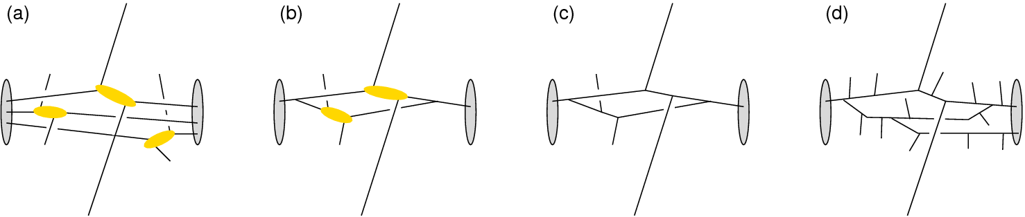
Figure 12: Contributions to the underlying event: (a) multiple $2\to 2$ interactions, (b) collinear splitting in the initial-state followed by double $2\to 2$ scattering, (c) perturbative, 1-loop, $2\to 4$ diagram, and (d) BFKL-type emissions.

In order to understand why UE is different from MB, let us examine Fig. 12, which depicts some of the sources of the underlying event taking dijet production as an example. In Fig. 12 (a) the hard interaction in which the dijet system is produces, is supplemented by multiple, independent, lower-$p_{T}$, $2\to 2$ scatterings. Such mechanism, called the multi-parton interactions (MPI) turns out to be responsible for a large fraction of the underlying event. Because the incoming particles all originate from the same proton, it is natural to expect that the individual $2\to 2$ scatterings shall be correlated both through the energy conservation or due to colour connections. Moreover, MPIs can be also realized via an alternative graph, shown in Fig. 12 (b), where both pairs of the incoming particles have in fact a common origin and arise from the initial-state collinear splitting.

However, the lowest order diagram corresponding to Fig. 12 (b), shown in Fig. 12 (c), can be regarded as a one-loop-double-real correction to the dijet process, which starts to be relevant at the order N³LO. Current modeling does not prevent us from double-counting between multiple parton interaction and perturbative higher orders [133, 134].

The soft radiation that fills the event is not bound to come just from the $2\to 2$ scatterings, but may also arise from configurations that involve BFKL-like, multiple chains of low-$p_{T}$ emissions spread in rapidity, as shown in Fig. 12 (d). Finally, additional radiation emitted from the initial-state particles (initial-state radiation, ISR) and the beam remnants will also contribute to the underlying event.

We see that it is general not conceptually clear how to separate the hard part, amenable to perturbative treatment, and the underlying, low-$p_{T}$ activity. One can turn the above statement around and say that because UE has a significant non-perturbative component, which cannot be calculated from first principles and can only be modeled, measurements of the underlying event are important as they provide a way to constraint parameters of phenomenological models.

To a first approximation, we expect that UE/PU modifies jet’s $J$ transverse momentum according to [135]

$$\langle\delta p_{T}(J)\rangle_{\text{UE}/\text{PU}}=\frac{\rho}{2}\left(R^{2}-\frac{R^{4}}{8}+{{\cal O}\left(R^{6}\right)}\right)\,,$$ (4.1)

where $\rho$ is an average transverse momentum per unit rapidity carried by the underlying event or pileup for a given event. A fully realistic correction needs to take into account the fact that jets are not exactly circular, but their areas depend on the algorithm and vary on the jet-by-jet basis. Therefore, the exact correction from UE/PU reads [136]

$$\langle\delta p_{T}(J)\rangle_{\text{UE}/\text{PU}}=\rho A(J)\pm\sigma\sqrt{A(J)}\,,$$ (4.2)

where $A(J)$ is an active jet area introduced in Section 2.5 and $\sigma$ is a standard deviation from the average UE/PU level, when measured across sub-regions of the event. Then, the transverse momentum of a jet can be corrected for the effects coming from UE/PU according to

$$p_{T}(J)^{\text{sub}}=p_{T}^{\text{measured}}(J)-\rho A(J)\,,$$ (4.3)

where $p_{T}(J)^{\text{sub}}$ is expected to correspond to genuine transverse momentum of the jet $J$.

Approaches to UE measurement

Measurements of the underlying event are on one hand important for jet physics, as they allow for corrections of jets’ transverse momenta and masses. On the other hand, jets themselves can be helpful in pining down the properties of UE.

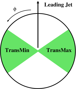
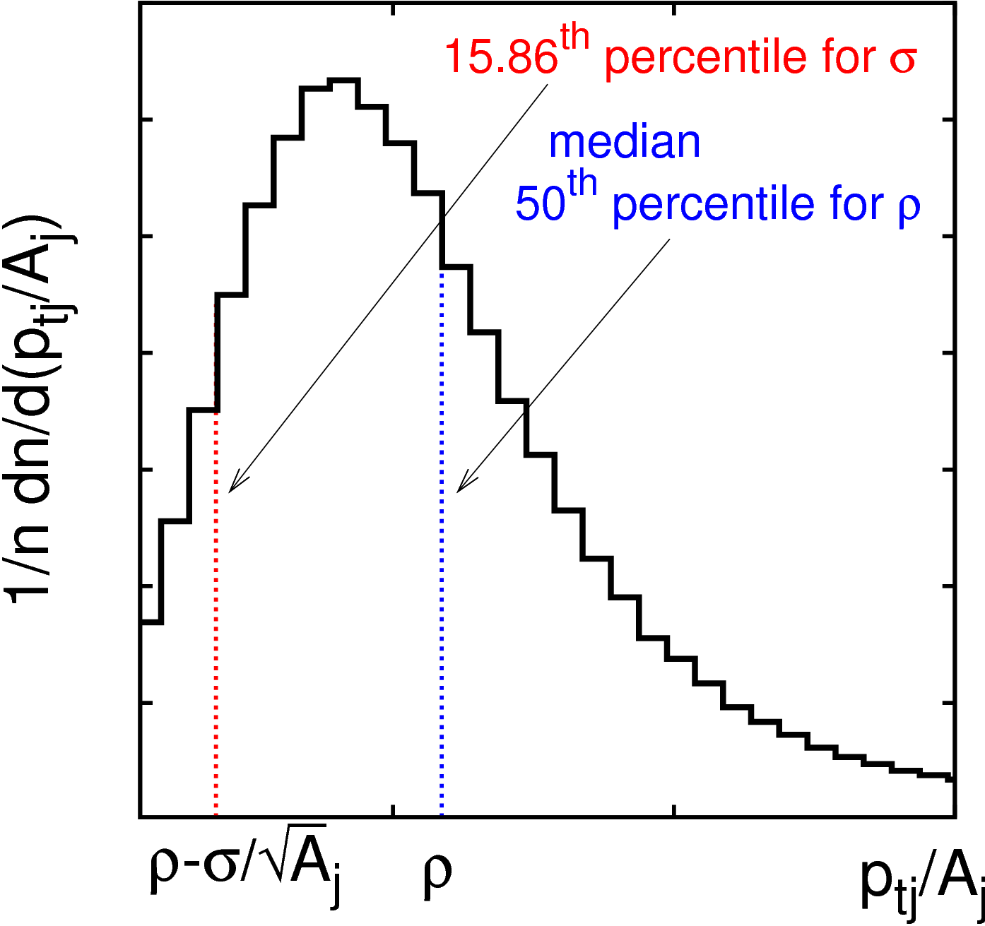
Figure 13: Methods of UE measurements. Left: traditional approach with the “TransMin” and “TransMax” regions in the transverse plane. Right: area/median based approach in which distribution of the transverse momentum over area, $p_{tj}/A_{j}$ for the set of jets in a single event is used to determine the average level of UE, $\rho$, and its standard deviation, $\sigma$. Figures from Ref. [137].

Traditional approach

The most widely spread approach [138] to measuring the properties of the underlying event involves tagging events based on the presence of a jet or a hard particle, and measuring the radiation separated from the hard object by the distance $\phi$ in the transverse plane. One defines four regions, as illustrated in Fig. 13 (left): the “towards” region, typically with $|\phi|<\pi/3$, the “away” region with $2\pi/3<|\phi|<\pi$, and two transverse regions, covering $\pi/3<|\phi|<2\pi/3$.

The idea behind this division is that most of the radiation generated in the hard scattering will occupy the towards and the away regions and, by measuring the activity in the transverse regions, one gets access to the genuine underlying event. Hence, one measures the multiplicity of charged tracks above some transverse-momentum threshold, as well as the total transverse momentum contained in the charged tracks, and typically presents the result as an average across many events and as a function of the $p_{T}$ of the leading jet.

The method is usually further improved by labeling the two transverse regions as “TransMin” and “TransMax”, respectively for the less and for the more active of the two, where the “activity” is defined with the total transverse momentum entering into the region. This is motivated by the fact that there is still a probability of order ${{\cal O}\left({\alpha_{s}}\right)}$ that one of the transverse regions receives radiation from the hard scattering, which significantly affects the extracted information about the average UE $p_{T}$ flow. The largest component of the perturbative contamination should contribute to the TransMax region, hence, by restricting the measurements to the TransMin region one reduced the bias from the hard radiation. The average over the two region is called “TransAv”.

The method gives freedom as to where exactly place the transverse regions, as well as to the choice of their size and shape. The LHC experiments tend to divide the transverse plane exactly at $|\phi|=\pi/3$ and $|\phi|=2\pi/3$, and consider jets or other hard objects with rapidities $|\eta|<2.5$ for measurements based on charged tracks [139]. UE measurements at Tevatron used the range o $|\eta|<1.0$ [140].

Jet-area/median approach

Another method to measure the underlying event and pileup, proposed in Refs. [136, 137], is based on the concept of jet areas [52]. In this approach, one first clusters the event with an IRC-safe jet algorithm, like C/A or $k_{T}$ and then attributes the active jet area, $A_{j}$ to each jet $j$, as described in Section 2.5. Notice that, because the active jet area is calculated by adding a large number ghost particles to the event, some jets will be formed uniquely from ghosts. Those are called the “pure ghost jets” and are considered to have $p_{T}=0$.

The key point of the method is to measure the transverse momentum density of per unit area in an event by taking the median of the distribution of the $p_{Tj}/A_{j}$ for the ensemble of jets in that event within certain rapidity window

$$\rho(y)=\mathop{\mathrm{median}}_{j\in\mathrm{jets},\;|y_{j}-y|<\delta y}\left[\left\{\frac{p_{Tj}}{A_{j}}\right\}\right]\,,$$ (4.4)

as shown schematically in Fig. 13 (right). The motivation for the use of the median is that it is much less susceptible to contamination from hard perturbative radiation, which is the main source of bias in the traditional approach.

The UE level, $\rho$, is measured on the event-by-event basis. In addition, one can also determine the intra-event fluctuations of the UE, $\sigma$, defined such that a fraction $X/2$ of jets satisfy $\rho-\sigma/\sqrt{\langle A_{j}\rangle}<p_{Tj}/A_{j}<\rho$, where $X$ is the fraction of a Gaussian distribution within one standard deviation of the mean [137]. As shown in Fig. 13 (right), this definition is one-sided (i.e. just considering jets with $p_{Tj}/A_{j}<\rho$). This helps to limit contamination of $\sigma$ coming from the hard jets when the total number of jets is small.

The jet area-based method is very robust when applied to both pileup and to UE measurements. The latter case is more challenging since the UE is softer, and has relative fluctuations that are larger than those in PU or MB. Hence, one faces the trade-off between getting the most differential information, by taking small rapidity windows in Eq. (4.4) and sensitivity to the hard contamination. If the rapidity window is too small, one has a limited number of jets that enter the formula (4.4) and the relative impact of the presence of a hard jet in the region of interest is amplified by the small total number of jets. One way to help in such situations, when studying UE in processes with $n$ jets is to remove the $n$ hardest jets from the list of jets used to compute the median.

The jet area-based method has been used by CMS to study the underlying event [141], where it has been also adjusted to cope with scarcely populated events. It has been also widely employed to the event-by-event UE subtraction for processes with photons [142, 143].

Experimental results of UE measurements

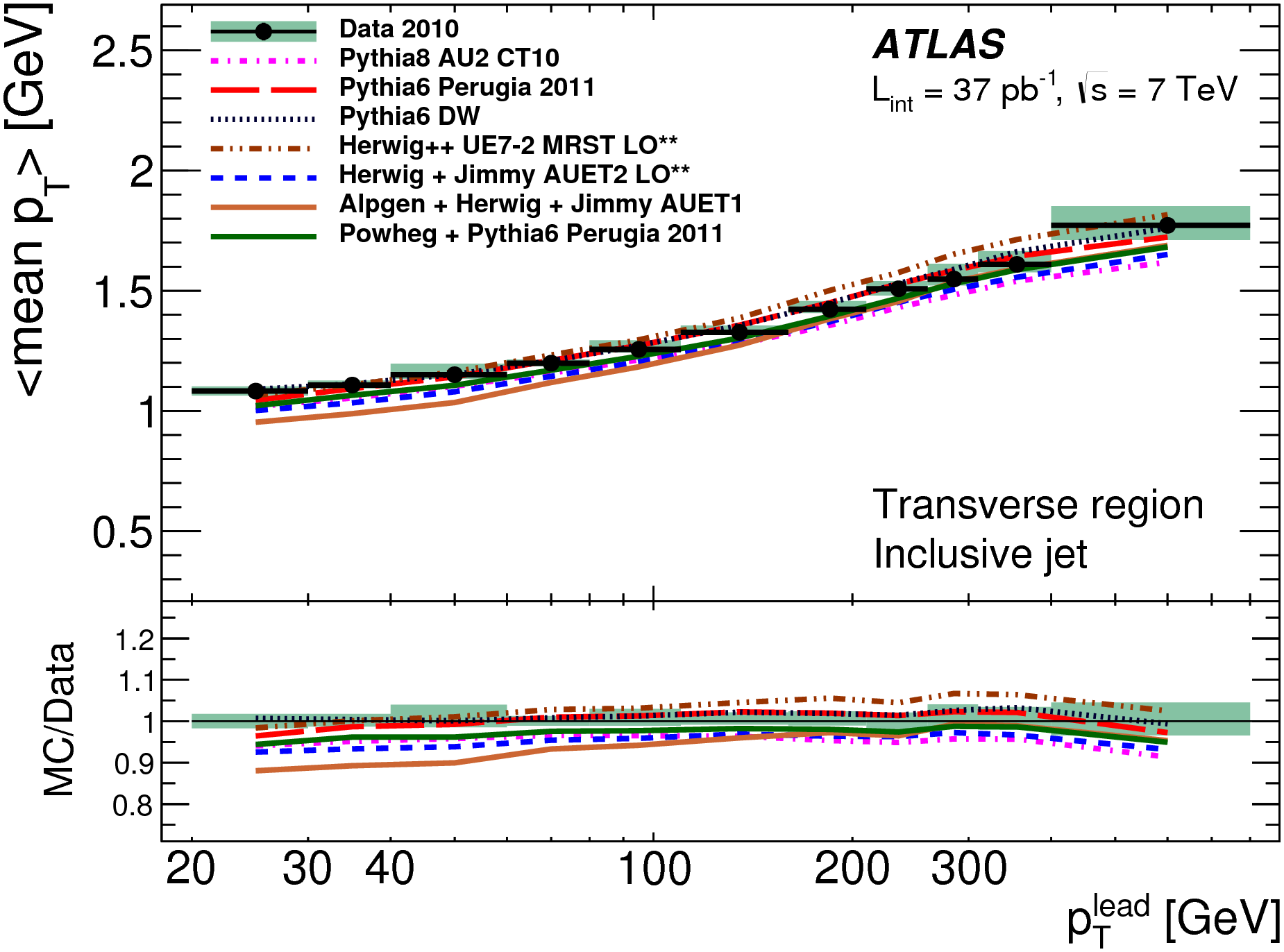
Figure 14: Transverse region profiles of the mean $p_{T}$ of charged particles for inclusive selection against the leading-jet $p_{T}$ compared to a range of MC models. The shaded area shows the combined statistical and systematic uncertainty. Figure from Ref. [144].

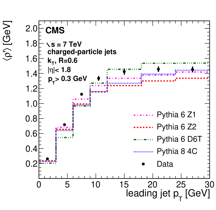
Figure 15: Mean values of $\rho^{\prime}$ distributions versus leading charged-particle jet transverse momentum compared to different generator tunes. Figure from Ref. [141].

A range of measurements of the underlying event have been performed since the start of the LHC and they have greatly helped to tune the MC models of soft and semi-hard radiation in this new energy domain.

Most of the results were obtain with the traditional method and using charged tracks as the leading hard objects[139, 145, 146] Complementary analysis, based on calorimeter information only, has also been performed [147]. This was an important cross-check as the neutral hadrons account for $\sim$ 40% of the produced particles.

The measurements covered the energies from $\sqrt{s}=900\,\text{GeV}$, through 2.76 TeV up to 7 TeV. Early UE measurements at 13 TeV start appearing now [148]. The qualitative features of the UE at higher energies remained the same as those found at Tevatron. That is, the UE in the TransAv region retains fairly strong dependence on the transverse momentum of the leading hard object, which is reduced in the TransMin region. The latter confirms the expectation that the TransMin region is less affected by hard radiation [144]. On the quantitative level, it turned out that none of the Monte Carlos tuned to the pre-LHC data was able to correctly predict the UE activity. The predictions for 7 TeV were lower than what has been found in the data, often up to 50%. In view of the above, the new UE data from ATLAS and CMS were used to retune model parameters [149, 144, 150]. The current status is that most of the modern tunes allow for 20% or better accuracy in the description of the ensemble of the UE characteristics, as shown in the example Fig. 15

The jet area/median based methods has also been used to study UE at $\sqrt{s}=0.9$ and $7\,\text{TeV}$ [141]. The original formula for $\rho$, given in Eq. (4.4), has been adjusted, by taking only the physical jets in the set used to determine the median, and the modified quantity was called $\rho^{\prime}$. This was motivated by the fact that, in the experimental situations with low average charged-particles multiplicities, the number of ghost jets is so large that $\rho=0$ in majority of cases.

Fig. 15 shows the mean value of $\rho^{\prime}$ measured by CMS, as a function of the transverse momentum of the leading jet, together with predictions from various MC tunes. The overall description is reasonably good, with the discrepancies at the level of 20% or lower. The observed sensitivity to UE modeling shows usefulness of the jet area/median approach in constraining models of soft radiation.

Further theoretical developments

The method of Ref. [136] for correcting jet transverse momenta for the contamination from UE/PU by using jet areas has been extended to the case of jet masses by introducing the concept of mass areas [53] as described in Section 2.6. The amount of mass coming from pileup, which needs to be subtracted from the jet mass, is given by [53]

$$\delta m^{2}(J_{\text{PU}})=p_{TJ_{\text{PU}}}\,\rho\,A_{m}(J_{\text{PU}})-\rho^{2}A_{\mu}^{2}(J_{\text{PU}})\,,$$ (4.5)

where $\rho$ is the level of UE/PU, $A_{m}$ is the active mass area while $A_{\mu}$ is the active jet area. The mass area is computed from uncorrected jets and the first term in Eq. (4.5) provides the leading contribution to the jet mass correction. Fig. 17 shows how the above procedure fares for a dijet production at the LHC. We see that, for events with pileup, the mass of a jet increases with the number of simultaneous collisions. By subtracting the first term of Eq. (4.5), one recovers the correct jet mass as long as the pileup is not too large. By adding the second term from Eq. (4.5), one obtains the correct jet mass even with large pileup.

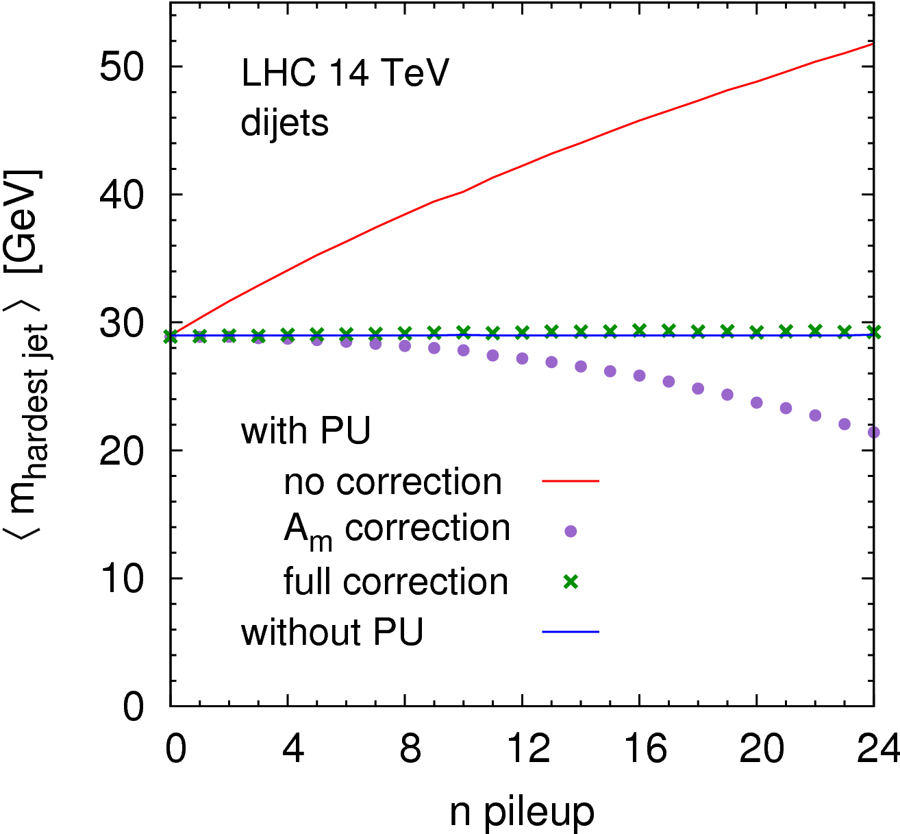
Figure 16: Average mass of the hardest jet in dijet events at the LHC. Jets were found with anti-$k_{T}$, $R=0.7$ and the cut $p_{T,\text{hardest}}>150\,\text{GeV}$ was imposed. Figure from Ref. [53].

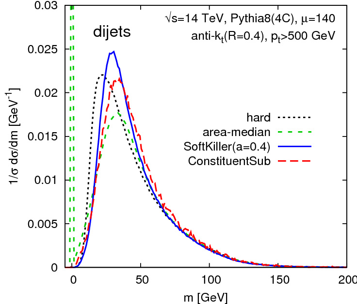
Figure 17: Performance of the Soft Killer and Constituent Subtraction methods as compared to the standard area/median subtraction for jet mass distribution. Figure from Ref. [151].

A somewhat related approach for measurement and subtraction of the incoherent energy flow (e.g. pileup) for massive jets has been proposed in Ref. [152]. It allows one to correct the jet mass, angularity and planar flow. The method is data-driven and it estimates the UE/PU activity, which should be subtracted from the jet, by summing energy in cones of the area $a_{0}=\pi R^{2}$ rotated by 90^∘ in the transverse plane with respect to the leading jet. The correction to the jet mass is found to have the form $\delta m\sim\sum_{i\in R^{90^{\circ}}}\frac{\delta m_{i}^{2}}{2m_{J}}$, where $i$ runs over particles in the cone perpendicular to the jet and the proportionality coefficient is found from a fit. The above functional dependence has been confirmed by fit to mass distributions measured by CDF.

A new jet shape variable, called the “angular structure function” was proposed in Ref. [153]. Its average over an ensemble of jets is defined as

$$\langle\Delta{\cal G}(R)\rangle\equiv R\frac{\sum_{k=1}^{N}\sum_{i\neq j}p_{Tk,i}p_{Tk,j}\Delta R_{ij}^{2}\delta_{dR}(R-\Delta R_{ij})}{\sum_{k=1}^{N}\sum_{i\neq j}p_{Tk,i}p_{Tk,j}\Delta R_{ij}^{2}\Theta_{dR}(R-\Delta R_{ij})}\,,$$ (4.6)

where $k$ runs through jets in the ensemble, $i,j$ label the constituents of the jet $k$ and $\Delta R^{2}_{ij}=(\eta_{i}-\eta_{j})^{2}+(\phi_{i}-\phi_{j})^{2}$ is the distance between two constituents in the transverse plane. $\delta_{dR}$ and $\Theta_{dR}$ are the Gaussian and error functions with the width $dR$. The quantity defined in Eq. (4.6) is a logarithmic derivative of the angular correlation function introduced in  Ref.[154] and the latter has an interpretation of the fractional mass contribution from constituents separated by the angular distance $R$ or less.

The angular structure function is formulated in terms of two-particle correlations and hence provides information complementary to the usual jet shapes. In particular, it receives contributions from uncorrelated radiation, hence it is sensitive to UE modelling and can be used to determine the level of the underlying event $\Lambda_{\text{UE}}$. As found in Ref. [153], $\Lambda_{\text{UE}}$ comes out very different for different Monte Carlo generators. The quantity $\langle\Delta{\cal G}(R)\rangle$ can be interpreted as an average scaling exponent with $\langle\Delta{\cal G}(R)\rangle=2$ for the leading order perturbative result. Most of the UE model give quasi-universal form of $\langle\Delta{\cal G}(R)\rangle\simeq 2$ at small R, which follows from the perturbative $2\to 2$ processes used to build up the MPI interactions. This feature can be directly compared with the experimental data.

A method for correcting the jet transverse momenta for the contamination from PU, called jet cleansing was proposed in Ref. [155]. It proceeds by rescaling the 4-momentum of each subjet, $p^{\text{tot}}_{\mu}$, by a factor determined from the constraint

$$p_{T}^{\text{tot}}=\frac{p_{T}^{C,\text{PU}}}{\gamma_{0}}+\frac{p_{T}^{C,\text{LV}}}{\gamma_{1}}\,,$$ (4.7)

where $p_{T}^{C,\text{PU}}$ and $p_{T}^{C,\text{LV}}$ are the transverse momenta of the charged particles coming from the leading vertex and pileup, respectively, while $p_{T}^{\text{tot}}$ is the total transverse momentum of a subjet. $\gamma_{0}=p_{T}^{C,\text{PU}}/p_{T}^{\text{PU}}$ and $\gamma_{1}=p_{T}^{C,\text{LV}}/p_{T}^{\text{LV}}$ are the ratios of the charged particles to all particles for the pileup and for the leading vertex. Hence, the method takes the input values for the charged particle transverse momenta, $p_{T}^{C,\text{PU}}$ and $p_{T}^{C,\text{LV}}$, as well as the total transverse momentum of a subjet, $p_{T}^{\text{tot}}$, to guess the ratio of $p^{\text{LV}}_{T}/p^{\text{tot}}_{T}$ and use it to rescale the measured $p^{\text{tot}}_{\mu}$ back to the original 4-momentum of a subjet formed uniquely from the leading vertex particles, $p_{\mu}^{\text{LV}}$. Depending on the assumptions on $\gamma_{0}$ and $\gamma_{1}$, one defines different variants of the cleansing procedure. The most sophisticated version, called “Gaussian cleansing” requires input from simulations but it is then able to rescale the jet four-momenta such that they reproduce the true value at the level of $\sim 98$% [155].

Several methods extending the original jet area/median-based approach have been proposed in recent years. In Ref. [156] the subtraction formula of Eq. (4.3) was generalized to any jet shape, $V$, and to higher orders in the pileup level parameters $\rho$ and $\rho_{m}$

$$V_{\text{jet},\text{sub}}=V_{\text{jet}}-\rho V_{\text{jet}}^{(1,0)}-\rho_{m}V_{\text{jet}}^{(0,1)}+\frac{1}{2}\rho^{2}V_{\text{jet}}^{(2,0)}+\frac{1}{2}\rho_{m}^{2}V_{\text{jet}}^{(0,2)}+\rho\rho_{m}V_{\text{jet}}^{(1,1)}\,,$$ (4.8)

where $V_{\text{jet}}^{(m,n)}$ denotes the $m^{\text{th}}$ derivative with respect to the ghost transverse momentum, $p_{T,g}$ and $n^{\text{th}}$ derivative with respect to the component $m_{\delta,g}=\sqrt{m_{g}^{2}+p_{T,g}^{2}}-p_{T,g}$. These derivatives can be determined numerically for a specific jet [156]. The PU levels are given by

$$\rho=\text{median}\left\{\frac{p_{T,\text{patch}}}{A_{\text{patch}}}\right\}\,,\qquad\qquad\qquad\rho_{m}=\text{median}\left\{\frac{m_{\delta,\text{patch}}}{A_{\text{patch}}}\right\}\,,$$ (4.9)

where the patches can be defined in various ways and Ref. [156] simply used the jets obtained with the $k_{T}$ algorithm with $R=0.4$. Applying the above general procedure results in the subtracted distribution returning very close to their original shapes with the second derivative playing a non-negligible role for certain processes like for example dijets. Also the $\rho_{m}$ component is shown to be important in some cases, notably for the filtered jet-mass distributions of fat jests in $t\bar{t}$ events.

The constituent subtraction technique [157] proceeds by applying the pileup correction to jet constituents rather then to the final jet momenta. Each event is populated with ghosts with $p_{T}^{g}$ proportional to the pileup density $\rho$. Then the transverse momenta of particles $i$ and ghosts $k$ are corrected iteratively following the procedure: If $p_{Ti}\geq p_{Tk}^{g}$: $p_{Ti}\to p_{Ti}-p_{Tk}^{g}$, $p_{Tk}^{g}=0$, otherwise $p_{Ti}\to 0$, $p_{Tk}^{g}\to p_{Tk}^{g}-p_{Ti}$, starting from the pair with the lowest $R_{ik}$ distance. Similar procedure is used to correct for the constituent masses. The method has been applied to dijet production and to $Z^{\prime}$ processes where it was shown to result in better mass resolution than the area based method and the shape expansion method [156]. An example of the performance is presented in Fig. 17.

Soft Killer method [151] for pileup removal has been proposed as a follow-up to the jet area based technique. It proceeds by eliminating particles with the transverse momenta $p_{T}<p_{T}^{\text{cut}}$ , where $p_{T}^{\text{cut}}$ is chosen as the minimal value that ensures that $\rho$ is zero, with $\rho$ defined as in Eq. (4.9) only that squared patches of size $a\times a$ are used instead of jets. The Soft Killer method exhibits similar, in the case of jet transverse momentum, or slightly larger, in the case of jet mass, bias than the area jet method, where the bias is defined as the difference between the value of $p_{T}$ or mass returned by the method and the true value. At this small expense, it brings however a significant, in some case as big as 30% improvement in the resolution of jet energy, mass and other jet shapes. Example comparison for the jet mass is shown if Fig. 17, where the peak resulting from the Soft Killer procedure is clearly the most pronounced.

Performance of the method is a function of the resolution parameter $a$. The optimal value of this parameter depends on jet radius and was found to be 0.4 for $R=0.4$ and 0.8 for $R=1$. Finally, Soft Killer brings nearly two orders of magnitude speed improvement as compared to the area/median method.

4.1.2 Hadronization

The other major non-perturbative effect relevant for jet production processes comes from hadronization. Contrary to UE/PU, hadronization corrections appear not only in the hadron-hadron collisions but also in DIS and ${e^{+}e^{-}}$.

According to the result of Ref. [135], hadronization changes jet transverse momentum by the average amount

$$\langle\delta p_{T}\rangle_{\text{hadr}}=\frac{2}{\pi}\left[-\frac{2C_{R}}{R}+{{\cal O}\left(R\right)}\right]{\cal M}\,{\cal A}(\mu_{I})\,,$$ (4.10)

where $C_{R}$ is the Casimir factor, equal to $C_{F}$ for the quark and to $C_{A}$ for the gluon jet, while ${\cal A}(\mu_{I})$ is an integral over a non-perturbative contribution to the strong coupling up to some infrared matching scale $\mu_{I}$. It is calculated as a difference between the average of the full coupling in the infrared region $\alpha_{0}(\mu_{I})\equiv 1/\mu_{I}\int_{0}^{\mu_{I}}{\alpha_{s}}(k_{T})dk_{T}$, and the perturbative contribution between the scales $\mu_{I}$ and $p_{T}$. The value of $\alpha_{0}(\mu_{I})$ is obtained from fits to DIS and ${e^{+}e^{-}}$ and it comes out around 0.5 for $\mu_{I}=2\,\text{GeV}$. The parameter ${\cal M}$ is called the Milan factor and it is an algorithm-dependent quantity with ${\cal M}\simeq 1.49$ for the anti-$k_{T}$ and ${\cal M}\simeq 1.01$ for the $k_{T}$ algorithm [158].

We see from Eq. (4.10) that the hadronization corrections are large and negative for small-size jets. With similar methods, one obtains corrections to the jet mass

$$\langle\delta m^{2}\rangle_{\text{hadr}}=\frac{4C_{R}}{\pi}p_{T}\left[R+{{\cal O}\left(R^{3}\right)}\right]{\cal M}\,{\cal A}(\mu_{I})\,,$$ (4.11)

whose dependence is not divergent in $R$, hence, the mass of small-$R$ jets is not as strongly affected by hadronization as their transverse momentum.

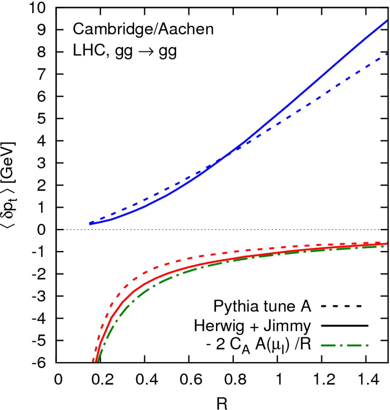
Figure 18: Modification of jet transverse momentum due to UE (upper curves) and hadronization (lower curves) for $qq\to qq$ scattering at the LHC, 14 TeV. Figure from Ref. [135].

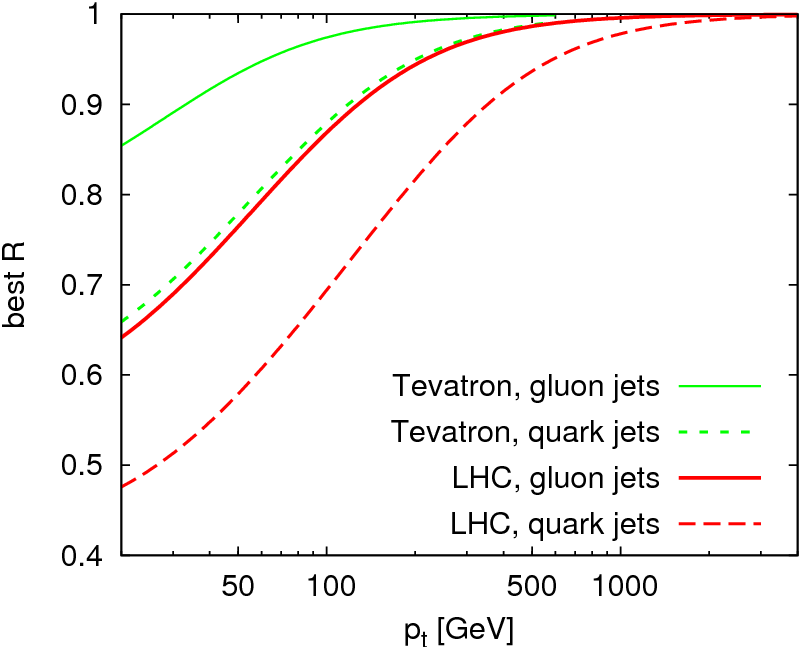
Figure 19: The value of jet radius, $R$, that minimises the sum of average, squared perturbative, hadronization and UE contributions as a function of jet transverse momentum. The level of UE per unit rapidity was taken at $\rho=4\,\text{GeV}$ for Tevatron and $\rho=10\,\text{GeV}$ for LHC. Figure from Ref. [135].

A summary of the nonperturbative effects coming from hadronization and underlying event is presented in Fig. 19. The upper curve corresponds to UE and we see that the change of jet’s momentum is positive and it becomes larger for large jets, which is qualitatively consistent with Eq. (4.1). On the contrary, the hadronization corrections are negative and their absolute value grows for small jets. Hence, the two have a chance to balance each other for moderate values of the jet radius $R\simeq 0.6$. In Fig. 19, the effects of hadronization are compared between the analytic calculations, taking just the leading order in $R$, as given in Eq. (4.10), and Monte Carlo results. We see that the two are very close to each other.

Let us conclude this section by noting that experiments use their own procedures to determine non-perturbative corrections from UE and hadronization (see for example Refs. [159, 23, 160]). The common practise is to rely on LO MC generators with LL showers. The corrections are calculated as bin-by-bin ratios of the MC cross sections obtained with and without modeling of hadronization and underlying event. They are determined using several generators and UE tunes. Then, an envelope of all correction factors is taken as a systematic hadronization+UE uncertainty. The final factors are subsequently used to multiply the parton level, perturbative predictions for jet observables.

The non-perturbative corrections determined that way [23] reach up to several percent and play an important role at low $p_{T}$ while significantly decreasing at large $p_{T}$. They depend on the jet radius and are mostly negative with the choice $R=0.4$ and positive with $R=0.6$. This is exactly consistent with the picture of the interplay between the UE and hadronization, and their respective dependence on jet radius, which we discussed above in the context of Fig. 19.

4.2 Choice of jet radius

Jet radius is a parameter of jet definition, c.f. Section 2.3. As discussed in the preceding subsection, the corrections to jet transverse momentum coming from UE/PU and those coming from hadronization behave differently with $R$. In addition to the above, there is also a purely perturbative mechanism that leads to further modification of jet’s $p_{T}$.

For any jet of size $R$, there will be a fraction of partons that are emitted outside of the jet area. The approximate perturbative formula for the corresponding transverse momentum loss reads [29]

$$\frac{\langle p_{T,\text{jet}}-p_{T,\text{parton}}\rangle}{p_{t,\text{parton}}}\simeq a\,{\alpha_{s}}\ln R\,,$$ (4.12)

where the prefactor $a=0.43$, if the parton that originated the jet was a quark, and $a=1.02$, if that parton was a gluon. We notice that when the jet radius is small, the transverse momentum (or energy) of the jet deviates significantly from that of the original parton.

By comparing Eqs. (4.1), (4.10) and (4.12), we see that the choice of a jet radius is a trade-off between different corrections, as the hadronization and leakage of perturbative radiation point towards larger jets, while the underlying event and pileup prefer smaller sizes. There are further reasons to be considered while choosing the jet radius. For example, if $R$ is large, than multiple, rather than a single hard structures end up inside a jet. This is sometimes useful, especially in the context of jet substructure analyses, c.f. Section 2.7, however, in standard measurements, one is typically interested in resolving each collimated energy flow into a single jet.

The values of jet radius used at the LHC range from $R=0.4-0.7$ for the proton-proton collisions [5, 7] and are usually smaller, around $R=0.2$, for the heavy-ion collisions [161]. The latter is motivated by very busy backgrounds.

Theoretical studies support the above choices adopted by the LHC experiments. Using the analytic or simulated results for the UE/PU contamination, hadronization effects and perturbative leakage, one can define the optimal radius as, for example, a value that minimizes the sum of the squared averages: $\langle\delta p_{T}\rangle^{2}_{\text{pert}}+\langle\delta p_{T}\rangle^{2}_{\text{hadr}}+\langle\delta p_{T}\rangle^{2}_{\text{UE}}$. The results, based on the analytic study performed in Ref. [135], as a function of jet $p_{T}$, are shown in Fig. 19. We see that the sizes which minimize the above sum depend on whether the jet originated from a quark or a gluon, with the latter preferring substantially larger jets. The average values are however in the range around $R=0.6$ for 100 GeV jets.

A more realistic Monte Carlo studies, with the so called quality measures [162], confirm the above pattern to a first approximation. Further details depend on the algorithm, type of the process, the parton initiating the jet, and the jet transverse momentum. Therefore, ideally, the jet radius should be chosen on the case-by-case basis.

Because the effects related to the choice of $R$ are non-trivial, they have been further studied both theoretically and experimentally. In Ref. [163] the ratios of the $p_{T}$ distributions in the inclusive jet production with two different values of jet radius, ${\cal R}(p_{T};R_{1},R_{2})=\sigma^{\text{NLO}}(pt,R_{1})/\sigma^{\text{NLO}}(pt,R_{2})$, have been computed in perturbative QCD and supplemented with non-perturbative corrections from hadronization following the prescription of Ref. [135]. Note that the leading order contribution to the inclusive jet spectra does not depend on $R$, as it involves only two partons recoiling against each other. For the same reason, the two-loop correction is also $R$-independent. That implies that the two-loop contribution, which is need for the NNLO jet cross sections, does not appear in the ratio ${\cal R}(p_{T};R_{1},R_{2})$ and one is able to obtain that quantity at the complete order ${\alpha_{s}}^{2}$ using just the NLO distributions. As found in Ref. [163], both the perturbative effects and the non-perturbative corrections are sizable at the LHC energies and the ratios ${\cal R}(p_{T};0.4,0.6)$ vary from 0.7 to 0.9 at low and high transverse momenta, respectively.

The measurement of the ratios of the inclusive jet cross sections with two different jet radius values, $R=0.5$ and $R=0.7$, has been performed by CMS [164] and compared to the result of Ref. [163]. It was found that the higher order and the non-perturbative correction are very important in obtaining the right shapes of ${\cal R}(p_{T};0.5,0.7)$ as a function of the transverse momentum in different rapidity bins. However, the NLO$\times$ non-perturbative corrections are still not entirely sufficient to exactly describe the measurements and better agreement is obtained with the matched calculations from Powheg + Pythia. This points to the relevance of higher multiplicities and resummation in precise description of jet ratios.

All order resummation of small-$R$ effects have been recently performed at the leading logarithmic accuracy, hence including the terms $({\alpha_{s}}\ln R^{2})^{n}$ [165]. The method exploits the angular ordering of the successive emissions in the range between the jet size $R$ and 1. Similar job is also done in practice by the standard MC parton showers, however, there, the small-$R$ corrections are entangled with other physical effects. The analytic approach of Ref. [165] allows for a robust estimate of the size of the small-$R$ corrections. Such result can be then combined with other calculations e.g. jet veto resummation, c.f. Section 4.4. The effects of the leading-logarithmic, all-order, small-radius resummation turn out to be sizable. For example, they can reduce the inclusive jet spectrum by 30-50% for jets defined with $R$ in the range 0.4-0.2, respectively. The expansion in $({\alpha_{s}}\ln R^{2})^{n}$ usually converges well for moderate-size jets but the all-order resummation is necessary for micro-jets of size $R\lesssim 0.1$. Such small jets are relevant in the context of the substructure studies, c.f. Section 2.7.

4.3 Perturbative calculations

We now turn to the perturbative calculations for jet processes. Those are crucial both for tests of QCD and for searches of new phenomena. We shall start with the cleanest possible approach in which the order of the strong coupling is fully controlled and fixed. Then, we will turn to frameworks where those fixed-order results are merged with each other or matched to a parton shower. As we elaborate on the stat-of-the-art theoretical results, we shall also discuss comparisons to selected distributions measured by the LHC experiments.

4.3.1 Fixed order calculations

All jet processes of interest have been calculated for hadron colliders up to NLO in QCD. Several of them have been recently pushed to the NNLO accuracy, although, in some cases only dominant contributions were included. Hence, significant work is still needed to make a complete transition from the current state-of-the-art of NLO to the desired NNLO accuracy. Below, we list and discuss at some length the fixed-order perturbative results for processes with jet production. Because the NLO calculations for many processes have been repeated several times with different methods and tools, it is impossible to cite them all here. Instead, we provide references to the first articles where the corresponding corrections were calculated, and, at the end of the section, we also give a list of modern tools which are used for phenomenological studies of jet processes at NLO. The complete, fixed-order literature can be gathered from there.

Pure jets

We start from the pure QCD jets, where the single inclusive results at NLO were obtained in Refs. [166, 167]. The most precise, complete theoretical calculations for dijets observables are currently also known at the NLO accuracy [168, 169]. Similarly, the three- [170, 171], four- [172] and five-jet [173] productions were calculated at NLO.

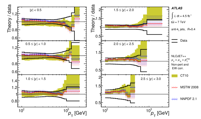
Figure 20: Ratio of NLO pQCD predictions to the measured inclusive jet transverse momentum distributions shown in bins of the jet rapidity, for anti-$k_{T}$ jets with R=0.4. The predictions were calculated using NLOjet++ [171] with different NLO PDF sets. Theory uncertainties include scale variations and PDF uncertainties and are given by the bands. The data lines show the total experimental uncertainty except the 1.8% uncertainty from the luminosity measurement. Figure from Ref. [23].

Single and multi-jet processes have been extensively studied at Run I of the LHC. In Fig. 20, we show the single inclusive jet spectra measured by ATLAS [23] presented as ratios to the NLO calculations from NLOjet++ [171] (see Ref. [23] for the corresponding cross sections). Similar measurement has been performed by CMS [9]. Overall good agreement, within, in some cases sizable, theoretical and experimental uncertainties is observed. Disagreement in the tails of distributions shows the potential for using jest to improve PDF fits. The dominant systematic experimental uncertainty comes from jet calibration. PDFs bring typically 10-20% uncertainty, much larger at large transverse momenta and masses.

The measurements of dijets cross sections and distributions have also been performed by ATLAS [23] and CMS [9]. Dijet invariant mass spectra have been compared to the fixed order NLO calculations and the level of agreement is comparable to that found in the single-inclusive distributions. The conclusion from the studies of three-jet mass distributions at 7 TeV  [160] is similar. Finally, distributions for the inclusive production of four jets have also been measured at the LHC at 7 [174] and 8 TeV [175]. Here, the LO $2\to$ ME+PS calculations describe the data poorly, while the fixed-order NLO results provide good description for virtually all distributions, bearing in mind that the experimental errors reach 30% at low momenta.

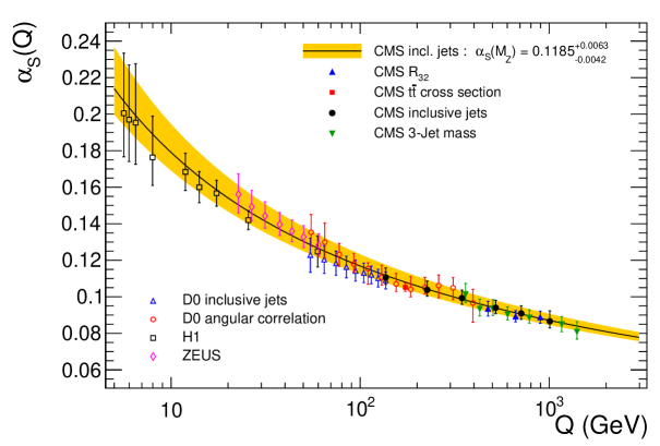
Figure 21: CMS measurements of the strong coupling in processes with jets at 7 TeV. Three different observables have been used: ratios of inclusive 3- to 2-jet distributions [176], single inclusive jet spectra [177] and 3-jet mass distributions [178]. Figure from Ref. [177].

CMS experiment has used jet processes to measure the strong coupling in several different ways. The first approach was based on studying the ratios $R_{32}$ of the inclusive 3-jet to the inclusive 2-jet cross sections at 7 TeV [176]. The ratio $R_{32}$ is proportional to ${\alpha_{s}}(Q)$, where $Q$ was taken as the average transverse momentum of two hardest jets. The measured ratio is compared to NLO predictions in which the ${\alpha_{s}}(m_{Z})$ value is varied and different PDF sets are used for calculations. The values of ${\alpha_{s}}(m_{Z})$ and ${\alpha_{s}}(Q)$, in various $Q$ bins, are determined by minimizing $\chi^{2}$. Differences between PDFs contribute to the experimental uncertainty. Another approach used the inclusive, 3-jet differential cross sections at 7 TeV [178]. With this approach, the strong coupling has been determined for scales between 0.4 and 1.4 TeV by minimizing $\chi^{2}$ and a combined fit for points above the 3-jet mass of $\sim 0.6$ TeV has been performed to determine ${\alpha_{s}}(m_{Z})$. Finally, inclusive jet measurements at 7 TeV were also used to measure ${\alpha_{s}}$ by employing a very similar methodology [177].

All of the above results of the strong coupling measurements are consistent with the renormalization group evolution and the value ${\alpha_{s}}(m_{Z})$ agrees with the world average. The CMS measurements of ${\alpha_{s}}$ are collected in Fig. 21, together with earlier measurements from Tevatron and HERA. As we see, jet-based determinations of the strong coupling provide direct results for ${\alpha_{s}}(Q)$ at scales from $\sim 0.1-2$ TeV.

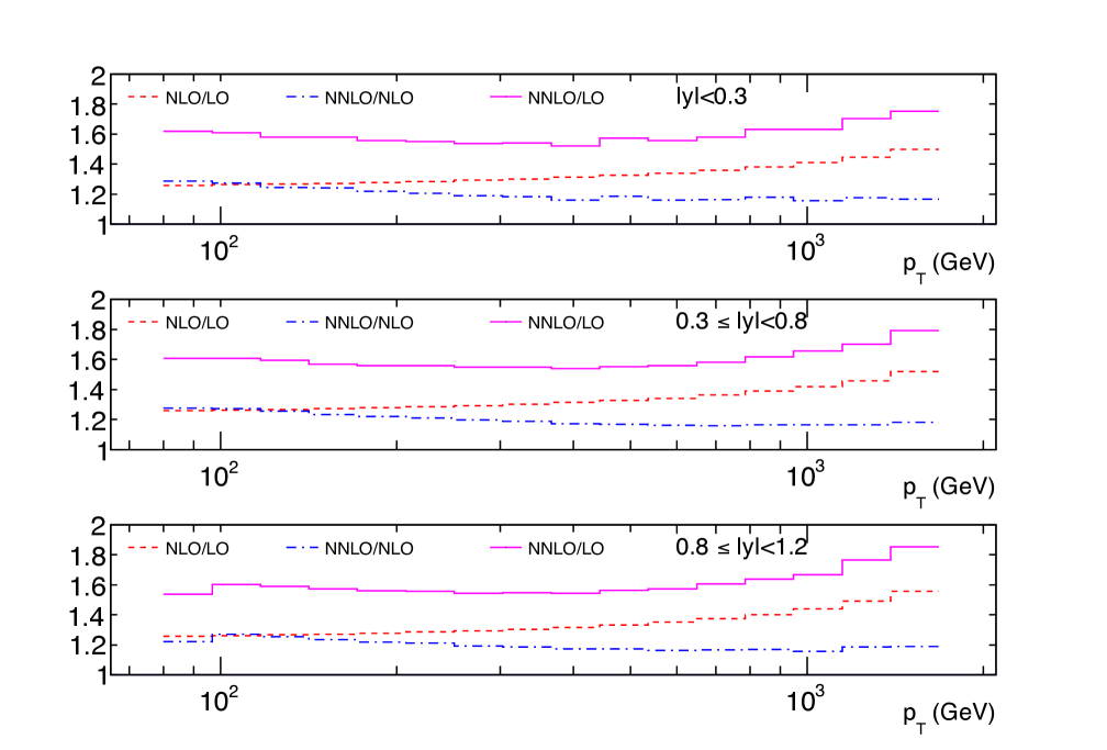
Figure 22: Ratios of the NNLO, NLO and LO cross sections for inclusive jet production, $d^{2}\sigma/dp_{T}$, in three rapidity slices. The results correspond to $\sqrt{s}=8$ TeV and the anti-$k_{T}$ jet algorithm with $R=0.7$. Figure from Ref. [179].

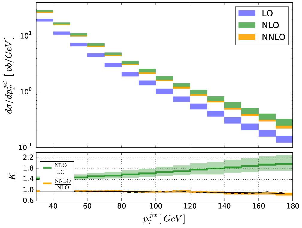
Figure 23: Transverse momentum spectra of the leading jet in $W$+jets process at LO, NLO and NNLO. The results correspond to $\sqrt{s}=8$ TeV and the anti-$k_{T}$ algorithm with $R=0.5$. Figure from Ref. [180].

Coming back to theoretical predictions, the NNLO result for dijet process has been recently obtained for the all-gluon channel. The calculation utilized the antenna subtraction method [181] and was first performed in the leading colour approximation [182] and later extended to the subleading colour [179]. In the antenna method, the subtraction terms are constructed from the so-called antenna functions, whose soft and collinear divergencies match those of the double-real, real-virtual and double-virtual contributions to the NNLO cross section. By adding the antenna functions and subtracting their integrated forms, one constructs the finite contributions from the $n+2$, $n+1$ and $n$-particle phase space, which are amenable to numerical integration. The study presented in Ref. [179] focuses on the comparisons of predictions at various orders of the perturbative expansion and between the leading and the full-colour results. A representative result is presented in Fig. 23, which shows the jet transverse momentum distributions for the single inclusive jet production in various rapidity bins. The NNLO/NLO K-factors turn out to be large, ranging between 16% and 26%. The picture is similar in all rapidity bins. The subleading colour terms contribute around 10% to the final result, in accordance with a naive power counting of colours, $1/N^{2}_{c}$.

Jets in association with electroweak bosons

Single vector boson production in association with one- [183] two- [184] three- [185, 186] four- [187] and five- [188] jets are known at the NLO accuracy in QCD. Very recently, the first NNLO results for the inclusive $W$+1 jet [180] and $Z$+1 jet [189] productions have been obtained.

The calculation for the $W$+ jets process has been performed with a new subtraction scheme based on the $N$-jettiness [190] variable $\tau_{N}$, which turns out to completely capture the singularity structure of QCD amplitudes with final state parton. This variable can be used as a resolution parameter to partition the phase space into the $N+1$-jet region, where the NLO result for $N+1$ production is used, and the $N$-jet region, where the missing NNLO contribution is obtained from the all-order, small-$\tau_{N}$ factorization formula derived within SCET [191].

As shown in Fig. 23, the NNLO corrections to the $W$+jet process turn out to be small and almost flat as a function of the leading jet transverse momentum. The scale uncertainty for that distribution is reduced from 20% at NLO to a few percent at NNLO. The total cross section decreases from NLO to NNLO by approximately 3%.

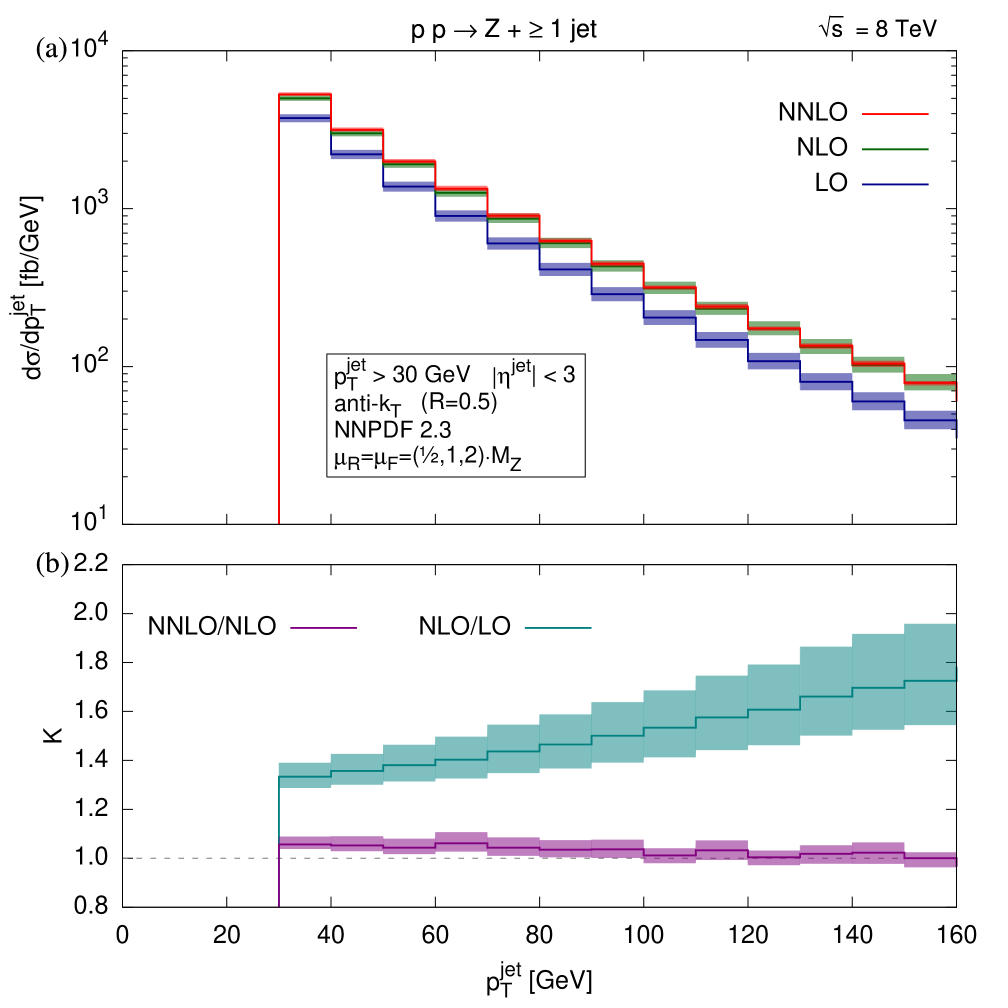
Figure 24: Distributions and corresponding K-factors of the leading jet transverse momentum in inclusive $Z$+jet production at $\sqrt{s}=8\,\text{TeV}$. Figure from Ref. [189].

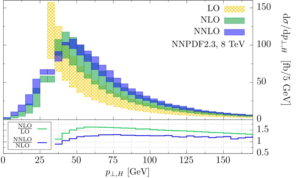
Figure 25: Higgs boson transverse momentum distribution in $H$+jet process at $\sqrt{s}=8\,\text{TeV}$. The bands correspond to renormalization and factorization scale variations around the central value taken at $\mu=m_{H}$. Jets are defined with the anti-$k_{T}$ algorithm with $R=0.5$. Figure from Ref. [192].

The $Z$+jets calculation has been performed in the framework of the antenna subtraction scheme [181] for the dominant $qg$, ${\bar{q}}g$, $q{\bar{q}}$ and $gg$ channels at leading colour. The distributions of the leading jet transverse momentum are shown in Fig. 25, where we see that, similarly to the case of $W$+jets, the NNLO correction is small, within 6% with respect to NLO, and the scale uncertainty is greatly reduced. The inclusive cross section raises by a similar amount.

Fully differential results are also available for the production of jets in association with the Higgs boson. The $H$+jet production is known at NLO [193] and NNLO [194, 195, 196]. The latter was calculated independently within three different approaches: the antenna method, the $N$-jettiness formalism and the Stripper method [197]. As an example, in Fig. 25, we show the differential distribution of transverse momentum of the Higgs. We see that the result stabilizes at NNLO. The central value still moves upwards by $\sim 20\%$ with respect to NLO but it stays inside the NLO uncertainty band. The scale uncertainty is significantly reduced at NNLO.

The $H$+2 jets process has been computed at NLO for the gluon fusion [198] and for the vector boson fusion (VBF) [199]. The latter has been recently upgraded to the NNLO accuracy [200] with a new “projection-to-Born” approach and it was found that the NNLO corrections to differential distributions can reach up to 10-12% with respect to NLO. The $H$+3 jets production is known at NLO for both the gluon fusion [201] and VBF [202].

As for diboson production in association with jets, $V_{1}V_{2}+n\,\text{jets}$, where $V_{1},V_{2}\in\left\{W^{\pm},Z,H,\gamma\right\}$, essentially all processes from this large group are known at NLO in QCD. This includes both the QCD-initiated production and the vector boson fusion. The results are differential in leptonic decay products and they account for spin correlations. The NLO corrections to those processes are sizable, typically in the range 10-40%, and they exhibit non-trivial phase space dependence. Detailed discussion of theoretical results for this class of processes, as well as the relevant references, can be found in Ref. [203].

It is clear from the above examples that the fixed-order calculations for the processes with jets are of crucial importance as the corrections found at NLO and NNLO are in many cases sizable. The current quest for the NNLO accuracy is well motivated as it is only this order that effectively allows one to reduce the theory uncertainties, coming from the unknown higher orders, down to a few percent level.

All of the differential calculations at NLO have been implemented in efficient numerical programs such as: Mcfm [204], Vbfnlo [205, 206], NLOjet++ [171], Sherpa [207], Njet [208], BlackHat [188], MadGraph5_aMC@NLO [209], GoSam [210] and OpenLoops [211]. In many cases, the calculations are fully automated. The complete list of processes possible to study with those tools, and the relevant references, can be found in the corresponding web pages.

In addition to the QCD higher orders, also the electroweak (EW) NLO corrections have been computed for several processes such as dijets [212], $W$+jet [213] and $Z$+2 jets [214]. The interplay between the radiative and the loop corrections has been analysed in Ref. [215]. The calculations for $W$+1 and 2 jets have been recently repeated in a fully automated setup and supplemented with that for the $W$+3 jets production [216]. These predictions include the orders ${\alpha_{s}}^{n+1}\alpha_{\text{EW}}$ and ${\alpha_{s}}^{n}\alpha_{\text{EW}}^{2}$ for the $W^{+}+n\,\text{jets}$ production processes. Notice that separation of the NLO corrections into the QCD and EW type is in general ambiguous. For example, ${{\cal O}\left({\alpha_{s}}^{2}\alpha_{\text{\sc ew}}^{2}\right)}$ can arise as a NLO correction to the $W$+2 jets production obtained by inserting an electroweak particle into the squared, tree-level diagram with an $s$-channel gluon emission. The same order, however, can be obtained by inserting a gluon into an interference diagram between the tree level amplitudes with the gluon and the electroweak boson, $s$-channel exchanges, respectively.

The mixed QCD EW results depend in a nontrivial way on observables as well as jet multiplicities. For example, the NLO QCD+EW corrections to the $W$+1 jet production at the LHC at 13 TeV [216] turn out to be negative for the distributions of $p_{T,W}$ but positive for the $p_{T,\text{leading jet}}$ distributions. The NLO QCD+EW corrections to the distributions of transverse momenta of the vector boson as well as the leading and subleading jets come out negative for $W$+2 and $W$+3 jets, with significantly smaller uncertainties than in the $W$+1 jet case. As for the dijet production [212], the pure weak loop corrections, ${{\cal O}\left({\alpha_{s}}^{2}\alpha_{\text{\sc ew}}\right)}$, to the distributions of the leading and subleading jets are negative, in the range of $-$12-16% at high $p_{T}$. They partially cancel with the LO EW ${{\cal O}\left({\alpha_{s}}\alpha_{\text{\sc ew}},\alpha_{\text{\sc ew}}^{2}\right)}$ contributions but the degree of cancellation depends on observable and the net effect can still reach $\sim 10\%$ in tails of distributions.

Processes of jet production in association with electroweak bosons have been extensively studied at the LHC. The most recent results include $Z$+jets [217, 218] and $W$+jets [219, 220]. We shall discussed them in the next subsection together with the matched and merged predictions.

4.3.2 Matching and merging for multi-jet processes

The predictions for multi-jet processes calculated within the fixed-order perturbative approach, described in the previous section, are invaluable. However, the complexity of those calculations increases very quickly when moving to higher orders and higher numbers of jets. This means that, within fixed-order pQCD, we can effectively model our final state with just a handful of quarks and gluons. Moreover, often only the inclusive cross section is available, with no access to the final state kinematics.

For those cases where the differential distributions are available, the fixed-order approach works reliably only at the high transverse momentum and fails as $p_{T}\to 0$. This is because of the large logarithms, $\ln p_{T}$, which compensate the small coupling at low $p_{T}$ and yield ${\alpha_{s}}\ln p_{T}\sim 1$. Hence, in the region of small $p_{T}$, each order contributes comparably and the logarithmic terms should resummed. One way to achieve the latter is provided by the parton shower (PS) approach, which sums the dominant, leading-logarithmic (LL) contributions, $({\alpha_{s}}\ln p_{T})^{n}$, as well as a subset of sub-leading corrections, to all orders. The events simulated with parton showers are fully exclusive and contain abundance of final-state partons. The distributions are however computed in the collinear (small-$p_{T}$) approximation, hence they differ from the exact results at high $p_{T}$.

The complementary advantages of the NLO calculations and the parton shower can be used simultaneously in a combined framework that goes under the name of NLO+PS matching. For processes with $n$ tagged jets, matched result are NLO-accurate for $n$-jet observables, LO accurate for $n+1$-jet observables and parton shower accurate for $n+1,n+2,\ldots$-jet observables. Such results can be further improved by correcting the vertices for the 2${}^{\text{nd}},3^{\text{rd}},\ldots,n^{\text{th}}$ emission with the exact NLO results for higher multiplicities. This procedure, called NLO merging, has to be, however, implemented carefully in order to remove all the double counting between contributions from samples with different multiplicities and to minimize dependence on merging parameters.

This section is devoted to discussion of the main methods for multi-jet matching and merging at NLO as well as NNLO. Examples of comparisons with LHC data are also discussed.

MC@NLO

was historically the first successful, general method of NLO+PS matching [98] (for earlier proposals see Refs. [221, 222]). The procedure starts by generating an emission according to the cross section

$$d\sigma=\Big{[}B(\Phi_{B})+\hat{V}(\Phi_{B})+\int K^{\text{MC}}(\Phi_{B},\Phi_{1})d\Phi_{1}\Big{]}d\Phi_{B}+\Big{[}R(\Phi_{B},\Phi_{1})-K^{\text{MC}}(\Phi_{B},\Phi_{1})\Big{]}d\Phi_{B}d\Phi_{1}\,,$$ (4.13)

where $B(\Phi_{B})$ represents the Born contribution over the phase space $\Phi_{B}$, $\hat{V}$ is a virtual term (before subtraction of soft and collinear divergencies), $R(\Phi_{B},\Phi_{1})$ gives the real correction with extra emission over the phase space $\Phi_{1}$, and $K^{\text{MC}}(\Phi_{B},\Phi_{1})$ is a kernel of the shower, which is a PS-specific approximation to the real term, hence, converging to $R(\Phi_{B},\Phi_{1})$ in the collinear limit. An event generated according to the cross section (4.13) has either $n$ or $n+1$ particles in the final state. The first case corresponds to the Born or virtual configuration and it is represented by the first term in Eq. (4.13). These events are called $\mathbb{S}$-type. The second case corresponds to a real, resolvable emission and it is given by the second term of in Eq. (4.13). Such events are called $\mathbb{H}$-type. In either case, the event is passed to the parton shower, which generates subsequent emissions in the collinear approximation.

With the integrated and unintegrated $K^{\text{MC}}(\Phi_{B},\Phi_{1})$ functions, Eq. (4.13) has a structure of the NLO subtraction formula [223]. Hence, the NLO accuracy of MC@NLO is manifest.

Since the definitions of the MC counterterms depend on the shower, those terms need to be calculated case by case. Currently, the MC@NLO matching can work with parton showers from the following generators: Sherpa [207], Herwig7 [224], which both use the dipole showers based on the Catani-Seymour subtraction scheme, hence, the NLO subtraction terms are identical to the kernels of the shower, and MadGraph5_aMC@NLO [209], which is capable of performing the matching with Herwig, Herwig7, Pythia6 and Pythia8 showers.

Recently, the MC@NLO method has been also worked out for the Nagy-Soper (NS) shower [225] in Ref. [226]. The potential advantage of the NS shower is that it includes soft effects at subleading colour, as well as spin correlations. The shower is currently implemented in Deductor [225] in the so-called LC+ approximation. The above code has been used together with Helac-NLO [227] to construct the matched samples. The implementation has been validated by studying the inclusive $t\bar{t}+\text{jet}$ production and comparing it to other matched results as well as to pure NLO. For observables insensitive to the shower, the matched results recover fixed order NLO distributions. For those sensitive to the soft and collinear radiation, results differ between various showers. The differences between NG and LL showers are however similar to the differences among various LL showers.

Together with Powheg, the Mc@NLO method has become a standard for matched calculations in QCD. It has been applied to numerous processes with jets, including the highly non-trivial cases of dijets [228] and W + up to three jets [229]. Mc@NLO is currently implemented in MadGraph5_aMC@NLO, Sherpa and Herwig7, and we point the Reader to those tools for further references and examples of applications to phenomenology.

Powheg

matching method [99] generates the first emission according to

$$d\sigma=\bar{B}(\Phi_{B})\left[\Delta_{S}(\mu_{0},\mu)+\Delta_{S}(p_{T},\mu)\frac{R^{S}(\Phi_{B},\Phi_{1})}{B(\Phi_{B})}d\Phi_{1}\right]d\Phi_{B}+R^{F}(\Phi_{B},\Phi_{1})\,d\Phi_{R}\,,$$ (4.14)

where

$$\bar{B}=B+\hat{V}+\int R^{S}d\Phi_{1}\,,\quad R=R^{S}+R^{F}\,,\quad\Delta_{S}(p_{T},\mu)=\exp\left[-\int_{p_{T}}^{\mu}\frac{R^{S}}{B}d\Phi_{1}\Theta(k_{T}(\Phi_{1})-p_{T})\right]\,.$$ (4.15)

The real contribution is split into the singular, $R^{S}$, and finite, $R^{F}$, parts in the small $p_{T}$ limit, and only the former is exponentiated in the Sudakov form factor $\Delta_{S}(p_{T},\mu)$. The scale $\mu_{0}$ separates the non-resolvable and resolvable emissions whereas $\mu$ is the uppers scale of the shower.

The Powheg formula for the first emission (4.14) is essentially a matrix element correction (MEC) [221] with the replacement $B\to\bar{B}$ and the splitting of the real part into $R^{S}$ and $R^{F}$. The former achieves full NLO accuracy of the matched result [230] whereas the latter avoids generation of spurious contributions from exponentiation of finite NLO terms that are unrelated to the all-order resummation of the collinear limit, which is effectively achieved by the Sudakov form factor. For further details on Powheg and MC@NLO, as well as for discussions of differences between these two methods, we refer to [230, 231]. As in the case of MC@NLO, the first emission in Powheg, generated with Eq. (4.14), is passed to a parton shower, which supplements the event with subsequent emissions in the leading logarithmic approximation.

The Powheg method is available in PowhegBox [232] and Herwig7 [224]. It has been used to calculate numerous predictions for processes with jets including dijet production [233], three-jet production [234], $Z$+jet [235], Z/$W$+2jets [236, 237], $t\bar{t}$+ jet [238] and $H$+1,2 jets [239].

KrkNLO

approach [95, 96] was constructed with the aim to maximally simplify the NLO+PS matching procedure. As discussed in the original articles [98, 99], both MC@NLO and Powheg are designed to work with $\overline{\text{MS}}$ PDFs. This is convenient in the context of the fixed-order calculations, however, it leads to a class of purely collinear terms in the partonic cross section, which need to be included in the MC shower generators aiming at achieving the NLO accuracy. That is problematic as the Monte Carlo produces particles in three, space dimensions and forcing it to generate partons in the strictly collinear phase space is not straightforward.

The KrkNLO method circumvents this problem by departing from the $\overline{\text{MS}}$ scheme into a new factorization scheme, called the Monte Carlo (MC) scheme, discussed at some length in Section 3.2. In the MC scheme, all the problematic, collinear contributions are essentially moved to the parton distribution functions that now become the new, MC PDFs. The latter can be obtained from the $\overline{\text{MS}}$ PDFs using Eqs. (3.14) and (3.15).

The method can be used with any shower whose coverage of the phase space of real emission is complete. Then, it boils down to correcting the hardest emission via reweighing with $W_{R}=R/K$ (notation of Eq. (4.13)) and multiplying the result by the $(1+W_{V})$. Here, $W_{R}$ is a weight related to the real radiation and it corrects the PS matrix elements, $K$, valid in the collinear approximation, to the exact matrix elements, $R$. The virtual weight, $W_{V}$, is a constant in the KrkNLO approach, as all the $z$-dependent terms are contained in the MC PDFs. The KrkNLO technique has been so far implemented for the Drell-Yan process [96] and the results are in general close, within $\sim 20\%$, to those from Powheg and MC@NLO. They are also closer to the complete NNLO prediction than the pure NLO and other matched calculations.

Geneva

method [240, 241] achieves matching at the NNLO+PS accuracy. Moreover, for some observables, the NNLO accuracy can be extended by resummation up to the order NNLL’ from SCET [242]. The key feature of this approach is a use $N$-jettiness [190], $\tau_{N}$, as a resolution variable which measures the degree to which the final state is a $N$-jet state. The limit $\tau_{N}\to 0$ corresponds to events with exactly $N$ infinitely narrow jets, while $\tau_{N}\gg 0$ occurs for the events with additional hard radiation between $N$ jets. Hence, $N$-jettiness can be used for phase space slicing, similarly to case of the fixed-order calculations discussed earlier.

The starting point of the Geneva approach is the inclusive, $N$-jet cross section given by

$$d\sigma_{\geq N}=d\Phi_{N}\frac{d\sigma}{d\Phi_{N}}\left(\tau^{\text{cut}}_{N}\right)+d\Phi_{N+1}\frac{d\sigma}{d\Phi_{N+1}}\left(\tau_{N+1}^{\text{cut}}\right)\theta\left(\tau_{N}-\tau^{\text{cut}}_{N}\right)\,,$$ (4.16)

with the first term bringing the exclusive $N$-jet cross section at a given fixed-order accuracy + resummation (currently, NNLO+NNLL’ for DY [241]) while the second terms corresponds to the inclusive $N+1$-jet cross section at an accuracy available for a given process (NLO+NNLL’ for DY).

The fixed-order+resummation formula (4.16) matches naturally to a shower ordered in the $N$-jettiness variable. One simply needs to generate the radiation via probabilistic shower algorithm and impose the condition $\tau_{N}<\tau_{N}^{\text{cut}}$ for the first emission from the $N$-jet event and $\tau_{N+1}<\tau_{N+1}^{\text{cut}}$ for the first emission from the $N+1$ event. Then, each subsequent emission needs to satisfy $\tau_{N+1}<\tau_{N+1}^{\text{cut}}$. One has to be slightly more careful when interfacing Geneva to showers ordered in variables other then $N$-jettiness. In practice, the first emission is done within Geneva, with the $N$-jettiness-ordered shower, which guarantees that it has the largest value of the jet resolution scale. Then, an event is passed a standard parton shower, e.g. from Pythia8, and a veto technique is used to ensure that subsequent emissions have lower resolution scales. As discussed in Ref. [241], such a procedure preserves the original accuracy of Eq. (4.16). As mentioned earlier, the Geneva method has been implemented and validated for the Drell-Yan process at NNLO+NNLL’ but the framework is capable of handling NNLO+PS matching for processes with final states jets.

LoopSim

method [243] allows for consistent mergings of NLO samples with different multiplicities.

The approach is based on the unitarity requirement, which leads to the condition that, at each order in $\alpha_{s}$, the singularities of the loop diagrams must be canceled by the singularities of the integrated real diagrams. This allows one to extract the singular structure of the missing loop contributions from the real diagrams with higher multiplicities.

The main ingredient of the method is a procedure for taking events with $n$ particles in the final state and supplementing them with all ($n-k$)–particle events (or equivalently all $k$-loop events), where $n$ and $k$ depend on the specific process and the order that we want to calculate. Because of unitarity, the sum of the weights of the full set of the above events will be zero. However, due to reshuffling of the weights between different bins and because of acceptance cuts, the contributions to the differential distributions will be finite. The LoopSim procedure consists of several steps in which the branching structure and the underlying hard structure are assigned to the original event, with the help of jet clustering algorithms with radius $R_{\mathrm{LS}}$. Then, the QCD partons that were not identified as final state particles are made virtual by recombining them, in all possible ways, with the emitters.

The jet radius $R_{\mathrm{LS}}$ is a parameter of the LoopSim method. The smaller the value of $R_{\mathrm{LS}}$, the more likely the particles are recombined with the beam. Reversely, the larger $R_{\mathrm{LS}}$, the more likely the particles are recombined together. The value of $R_{\mathrm{LS}}$ is irrelevant for the collinear (or soft) radiation. It affects only the wide-angle (or hard) emissions, where mergings between particles compete with the mergings with the beam.

The difference between the exact NNLO distribution for an observable $A$ and the LoopSim approximation seats in the finite constant associated with the two-loop diagrams. Since, the latter have LO topology, the difference becomes very small for distributions with significant NLO K-factors and goes as $\sim{\alpha_{s}}^{2}/K^{(A)}_{\text{NNLO}}$, where $K^{(A)}_{\text{NNLO}}=\sigma^{(A)}_{\text{NNLO}}/\sigma^{(A)}_{\text{LO}}>K^{(A)}_{\text{NLO}}=\sigma^{(A)}_{\text{NLO}}/\sigma^{(A)}_{\text{LO}}\gg 1$. Therefore, differential distributions sensitive to new channels and new, kinematically enhanced configurations, which lead to large NLO K-factors, are very close to the full NNLO result.

The method has been used for a variety of processes at hadron colliders including DY [243], $W/Z$+jets [244], dijets [243] and dibosons [245, 246, 247]. In particular, in Ref. [244], the predictions for the $W$+jets and $Z$+jets production have been compared to the 7-TeV LHC data. There, it was found that the description of the data for the distributions of the leading jet transverse momentum with the LoopSim-simulated NNLO result is comparable to that of NLO. However, the LoopSim predictions exhibit significant reduction of scale uncertainties. On the other side, the $H_{T}$-type distributions obtained with LoopSim agree much better with the 7-TeV LHC data than NLO [244].

MiNLO

method [248, 249] can be regarded as NLO extension of the CKKW [250] procedure. The latter is an algorithm for merging tree level events with different multiplicities and matching them to a parton shower. This provides a unified framework valid both in the wide-angle, multi-jet region (domain of the Born cross sections) and in the collinear region (domain of the shower).

The MiNLO method for merging the NLO samples with $N+0,N+1,\ldots,N+n$ jets, where $N$ is the minimal number of jets required in the process of interest, proceeds as follows: Each event, calculated at the scale $Q$, is re-clustered with the $k_{T}$ algorithm in order to reconstruct the most probable branching history. If the clustering results in $N$ jets, we call that configuration a $N$-jet primary system. The lowest order, tree level, $N$-parton contribution to the primary system is in general proportional to ${\alpha_{s}}^{m}$, where $m\geq N$. For example, $m=N=2$ for dijet production but $m=2>N=0$ for the Higgs production in gluon fusion. Hence, the tree event with $N+n$ partons is proportional to ${\alpha_{s}}^{m+n}$, while the real and virtual events are proportional to ${\alpha_{s}}^{m+n+1}$.

To each of the first $n$ vertices, $i=1,\ldots,n$, where the lower value corresponds to earlier time in the branching history of forward evolution, one assigns a scale $q_{i}$, equal to the relative transverse momentum at that branching. In the case of real events, the first clustering is associated with the scale $q_{0}$. Hence, the scales are ordered according to: $q_{0}<q_{1}<q_{2}<\cdots<q_{n}$. If $q_{n}>Q$, which may happen for example in the $Z$ production in association with a hard jet, one sets $Q=q_{n}$.

$n$ powers of of the coupling, those corresponding to the unresolved branchings, are evaluated at scales $q_{i}$ by reweighting the with the factors ${\alpha_{s}}(q_{i})/{\alpha_{s}}(Q)$. Another $N$ powers, those corresponding to the primary system, are evaluated at the scale $Q$. The choice of the scale in the $(m+n+1)^{\text{th}}$ power of the coupling is a delicate problem and prescriptions vary from case to case. In order to prove the formal NLO accuracy of the MiNLO result for production of a colour singlet, $V$, obtained by merging the $V$+0 and $V$+1 NLO samples, one needs to set the scale in that power of ${\alpha_{s}}$ to the value of the transverse momentum of $V$. This case corresponds to $N=0$. MiNLO has also been successfully used for processes with $N>0$ but, in those cases, no formal claim about the accuracy is made.

After the assignments of scales in all the powers of the strong coupling, the intermediate lines between the vertices are re-weighted with the Sudakov form factors. For real events, the external lines that join at the first node are not multiplied by the Sudakovs. In addition, one performs a subtraction of part of the NLO contribution already present in the CKKW Born term. For further details see Refs. [248, 249]. It is also worth to note that the MiNLO procedure does not involve a merging scale.

MiNLO has been used to study $W$, $Z$ and the Higgs boson productions in association with 0, 1 and 2 jets [248, 249]. The results were found to be well behaved in the Sudakov region for a large class of distributions, contrary to the pure NLO results, which are unstable in that region. Away from the Sudakov region, MiNLO performs similarly to a regular NLO. The results for $W/Z$+2 jets production have been also extensively compared to data in Ref. [237], finding a generally good agreement. Other interesting study focused on the $VH+0$ and $VH+1$-jet merging [251]. As this is an example of the production of a colour-neutral object, the result yields complete NLO accuracy.

The MiNLO method has been also used in conjunction with Powheg to achieve NNLO+PS matching for the Higgs production [252] and for Drell-Yan [253]. We recall that each of these processes, matched with Powheg at the NLO+PS level, is NLO accurate only for the inclusive observables, while the spectrum of the associated jet has LO accuracy. By using MiNLO to merge $V$@NLO+PS with $V$+jet@NLO+PS, one attains the NLO accuracy for the inclusive quantities simultaneously for the $V$ and $V$+jet processes, hence both the rapidity and the $p_{T}$ spectra of the boson are NLO-accurate. Such result can be subsequently reweighted in order to upgrade the inclusive boson production observables to NNLO, thus achieving the NNLO+PS matched result. As shown in Refs. [252, 253], by doing the above reweighting carefully, the NLO accuracy of the 1-jet observables is preserved.

MEPS@NLO

is also a method designed to consistently combine the NLO samples with different multiplicities and to match them to a parton shower [254]. Hence, it can be regarded as a variant of an NLO extension of the CKKW-L merging. In MEPS@NLO, the merging is achieved by combining the MC@NLO samples for various number of jets with help of a truncated parton shower. A Sherpa flavour of the MC@NLO method [231] is used to match each of the $(n+k)$-parton, NLO matrix elements to the parton shower individually. Here, $n$ denotes the number of QCD partons in the process of interest at the Born level.

A branching with the smallest hardness, characterized by the scale $Q_{n+k}$, in an event with $n+k$ final state partons, is used to separate events into different multiplicity classes. When $Q_{n+k}>Q_{\text{cut}}$, the event is called a $(n+k)$-jet event, otherwise it is labeled as a $(n+k-1)$-jet event. The parameter $Q_{\text{cut}}$ is called a merging scale. The real NLO events with $n+k+1$ partons are reduced to $n+k$-parton events by clustering.

If ${\cal O}$ is an arbitrary, infrared-safe observable, say a cross section for the production of a boson in a certain bin of $p_{T}$, then its $(n+k)$-jet exclusive expectation value to the order ${\alpha_{s}}$ is schematically given by [254]

$$\langle{\cal O}\rangle_{n+k}^{\text{excl}} \!\!\!\!\!=\!\!\!\!\! \int\!\!d\Phi_{n+k}\Theta(Q_{n+k}-Q_{\text{cut}})\tilde{B}\left[\Delta^{(A)}(t_{c}){\cal O}_{n+k}+\int\!\!d\Phi_{1}\frac{D^{(A)}}{B}\Delta^{(A)}(t_{n+k+1}){\cal O}_{n+k+1}\Theta(Q_{\text{cut}}-Q_{n+k+1})\right]$$ (4.17)

$$+\int\!\!d\Phi_{n+k+1}\Theta(Q_{n+k}-Q_{\text{cut}})\Theta(Q_{\text{cut}}-Q_{n+k+1})H^{(A)}\Delta^{(\text{PS})}(Q_{\text{cut}}){\cal O}_{n+k}\,,$$

where $\Delta^{(A)}(t)$ and $\Delta^{(\text{PS})}(t)$ are the Sudakov factors, hence the probabilities of no-emissions between the scale $t$ and the upper scale $\mu_{Q}$, with $t_{c}$ being an infrared cutoff. The two Sudakov functions differ by the kernel, which is provided by the subtraction terms $D^{(A)}$, or by the parton shower, respectively. The Sudakov factor of the second line assures no shower emissions in the $(n+k)$-jet region. The $\tilde{B}$ and $H^{(A)}$ functions are the analogues of the $\mathbb{S}$ and $\mathbb{H}$ terms of MC@NLO defined in the context of Eq. (4.13). The $\Theta$ functions guarantee that only the $(n+k)$-jet events contribute to the observable ${\cal O}$.

By combining the results obtained with Eq. (4.17) for a range of multiplicities between $n$ and $n+k$, we achieve the NLO-merged result matched to a parton shower. As demonstrated in Ref. [254], the method preserves both the NLO accuracy of the fixed-order, $n,n+1,\ldots,n+k$-multiplicity results and the logarithmic accuracy of the shower

The MEPS@NLO method has been used to study $W$+jets [254], four-lepton + 0 and 1 jets [255], $H$+jets [256] with a special focus on the analysis of uncertainties, as well as $t\bar{t}$ production with up to two jets [257] and to processes with multiple weak bosons  [258], the latter being relevant as a background to the associated Higgs production.

In the case of $W$+jets, significant decrease of the scale uncertainties is observed and an overall excellent agreement with ATLAS data is found. Similarly, MePs@NLO applied to $t\bar{t}$ + jets helps to reduce the uncertainties down to the level of 20%, compared to 50% observed in tree-level-merged distributions. Also, the four-lepton + 0 and 1 jets predictions profit from MePs@NLO merging as compared to pure NLO or Mc@NLO, both in terms of reduction in the scale uncertainties (in some cases even down to 5%), as well in improved tails of distributions and in the inclusive cross sections. On the contrary, for $H$+jets, no significant improvement in terms of the scale uncertainties in observed. This is attributed to the ${\alpha_{s}}^{2}$-dependence of the Born contribution as well as to the intrinsic parton-shower uncertainties and could probably only be improved by enhancing the accuracy of the shower.

UNLOPS and UN²LOOPS

methods [259, 260] not only upgrades the CKKW-L-type merging to NLO but they also restore unitarity of the merging procedure, which is not exactly satisfied in the original CKKW-L prescription.

When examined carefully [261], the CKKW-L method turns out not to preserve the inclusive cross section. This comes from a mismatch between the exact, tree level, $n$-jet matrix element and its parton shower approximation, with the latter entering through the Sudakov functions. A parton shower (in backward evolution) is unitary because the contribution corresponding to a jet being emitted at the scale $\rho$, integrated between $\rho_{0}$ and $\rho_{\text{max}}$, is cancelled with the contributions for no jets being emitted between the scales $\rho$ and $\rho_{\text{max}}$. This is however not true in a CKKW-L-merged result since, there, the higher-multiplicity samples are only added, while they should also be subtracted, in an integrated form, from the lower multiplicity states.

One of the consequences of unitarity violation is a residual dependence on the merging parameter through sub-leading logarithms of the merging scale cut. The UMEPS procedure [261] restores unitarity of the CKKW-L merging by supplementing it with the above, missing subtraction terms. This is done by using the exact, higher multiplicity states (rather than their parton shower approximation) to calculate the integrated contributions relevant for the resummation in the lower multiplicity samples. Then, the parton shower domain is pushed to multiplicities higher than what is provided by the exact tree level samples. And indeed, the above procedure allows for use of lower merging scales, which in turn improves description of certain observables at small $p_{T}$.

The UMEPS method was updated to the NLO merging in UNLOPS [259] by providing additional set of subtraction terms, related to the exact NLO contributions from higher-multiplicity samples. Around the same time, a similar approach was proposed in Ref. [260]. The UMEPS/UNLOPS methods have tight relation to LoopSim [243], with the integrated contributions in the former being analogous to the simulated loop contributions in the latter.

The results of merging of the $W/H$+ 0, 1 jet samples with UNLOPS show very small dependence on the merging scale [259] The ATLAS data for jet multiplicities varying from 0 to 4 are very well described by the UNLOPS predictions. A general tendency of producing the leading jet $p_{T}$ spectra with tails harder than what is seen in data is found.

The above method has been recently extended to construct a NNLO+PS matching procedure. The technique, dubbed UN²LOPS, was used for Drell-Yan [262] and Higgs production in gluon fusion [263]. The matching is performed with help of the $q_{T}$-subtraction method [264], where the phase space is sliced according to the value of the transverse momentum of the electroweak boson, $q_{T}$. All configurations with $p_{T,V}<q_{T}$ correspond to the zero bin and the NNLO cross section in that bin is most readily obtained within SCET [242]. Contributions from configurations above $q_{T}$ correspond to simple application of the NLO+PS merging procedure for the $Z/H$+1 jet process. After adding the above two contributions and subtracting the ${{\cal O}\left({\alpha_{s}}\right)}$ emission from the shower (to avoid double counting), one achieves the NNLO+PS matched result. The latter is found to be generally consistent with NNLO and superior over NLO+PS for a range of observables.

FxFx

procedure [265] was designed to merge MC@NLO results with different jet multiplicities.

As illustrated in Eq. (4.13), a given tree level matrix element $M_{n}$ contributes both to $n$-parton samples (via $\mathbb{S}$-type events) and to $n-1$ parton samples (via $\mathbb{H}$-type events). Hence, naive addition of the MC@NLO results with different multiplicities would lead to a clear double counting. The above problem can be solved by carefully vetoing emissions above or below a merging scale $Q_{\text{MS}}$. For example, in order to merge the 0- and 1-particle samples, one modifies the $\mathbb{S}$ and $\mathbb{H}$ contributions from the original MC@NLO prescription, Eq. (4.13), according to

$$d\sigma_{\mathbb{S},0}=B_{0}+\hat{V}_{0}+B_{0}\,K^{\text{MC}}\Theta(Q_{\text{MS}}-d_{1})\,, \qquad\quad d\sigma_{\mathbb{H},0}=\left[B_{1}-B_{0}\,K^{\text{MC}}\right]\Theta(Q_{\text{MS}}-d_{1})\,,$$ (4.18a)

$$d\sigma_{\mathbb{S},1}=\left[B_{1}+\hat{V}_{1}+B_{1}\,K^{\text{MC}}\right]\Theta(d_{1}-Q_{\text{MS}})\,, \qquad\quad d\sigma_{\mathbb{H},1}=\left[B_{2}-B_{1}\,K^{\text{MC}}\right]\Theta(d_{1}-Q_{\text{MS}})\,.$$ (4.18b)

The above formulae are of course only schematic and the notation is similar to that of Eq. (4.13), with $B_{i}$ corresponding to the $i$-parton, tree level contribution and $\hat{V}_{i}$ denoting the related (subtracted) virtual contribution. The $\Theta$ functions guarantee that the $(i+1)^{\text{th}}$, real emission, with the hardness $d_{1}$, does not, for $\sigma_{\mathbb{S},0}$ and $\sigma_{\mathbb{H},0}$, or does, for $\sigma_{\mathbb{S},1}$ and $\sigma_{\mathbb{H},1}$, contribute to the cross section. After such a slicing, the sum of the contributions from Eq. (4.18) provides a correctly merged result. Because of the $\Theta$ functions, the extra parton emitted on top of the $n$-particle sample is either always unresolved, Eq. (4.18a), or always resolved, Eq. (4.18b). This means that the combination of Eqs. (4.18) can be effectively regarded as a LO merging, which implies treatment similar to that of CKKW, i.e. each sample is reweighted with the Sudakov form factors (see Ref. [265] for detailed discussion).

The FxFx method has been validated for the Higgs production, $e^{+}\nu_{e}$ production, and $t\bar{t}$ production in hadron-hadron collisions, where the spectra were also compared to Mc@NLO and Alpgen. Theoretical uncertainties related to the merging were found to be small. Detailed discussion on subtelties of the choice of merging scales and further phenomenological studies for the dibosons and associated Higgs production can be found in Ref. [209].

A comprehensive study of the predictions from the FxFx method for multi-jet production in association with a vector boson has been recently presented in Ref. [266]. A range of differential distributions were compared the 7-TeV LHC results for the $W$+jets and $Z$+jets processes, as well as for the inclusive dilepton production. Theoretical results correspond to merging the NLO samples for $V$+1 jet and $V$+ 2 jets and matching them to the parton shower from Herwig7 and Pythia8. The study finds a good agreement between the predictions and the data from ATLAS and CMS. As expected, the merged NLO samples exhibit reduced scale uncertainties. Similarly to the result found in Ref. [244], also here, merging of the 0- and 1-jet samples does not bring the prediction for the leading jet $p_{T}$ distribution into full agreement with the data, although the experimental errors cover for most the difference. Description of the $H_{T}$ distributions, however, is greatly improved by the merged result from FxFx.

Electroweak merging

As discussed in Section 4.3.1, in addition to the NLO and NNLO QCD corrections, one should in principle always study the effects coming from the electroweak higher orders. This is also true in the case of parton showers. Consider the $W$ + 2 jets production at LO. Configuration with a hard $W$ boson recoiling against a quark or a gluon, while the other parton is soft, can be considered as a QCD correction to the $W$ production. Hence, it is expected to be well described by the standard merged results of the CKKW-L type for $W$ production + parton shower. If, however, in the same process, the two partons are hard, recoiling against each other, with one of them emitting a $W$ boson at small relative transverse momentum, then, it is more natural to describe such a configuration as a EW correction to dijet production. Moreover, because the $W$ boson is emitted at small angle, the above configuration should profit from resummation of collinear $W$ emissions. Hence, the second situation is expected to be well described by an analogue of the CKKW-L merging but for the dijet process + EW shower.

Ref. [267] proposed a prescription to merge the above two, merged results into a common framework with the EW and QCD showers. In such a result, the hard emissions of QCD partons, as well as the $W$ boson, are generated with the fixed-order matrix elements, while the soft emissions of partons and $W$s come from the QCD and EW showers, respectively. The method is currently worked out for the tree level merging and it is implemented in Pythia8. Detailed numerical studies for the LHC show that the new scheme improves most of the distributions as compared the standard CKKW-L prescription with a QCD shower only. The importance of the soft and collinear $W$ emissions grows with the center of mass energy. This is because, the higher $\sqrt{s}$, the more frequent the events with very hard partons. Therefore, the hierarchy of scales between the partons’ and the $W$ bosons’ transverse momenta increases and the resulting EW logarithms become more important. Indeed, as found in Ref. [267], the weak Sudakov effects for dijet production can be large and will become especially important at the future, 100 TeV proton collider, where they can reach up to 25% at $p_{T}$s of the order of 20 TeV.

Confronting theory and experiment

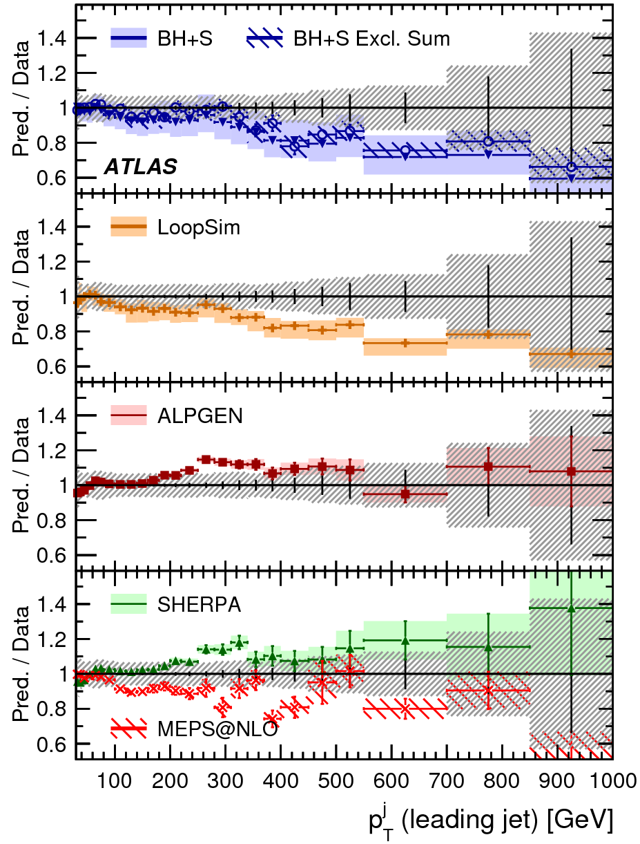
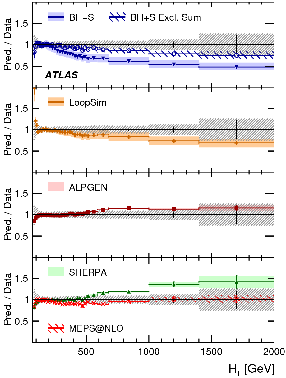
Figure 26: Cross sections for the production of $W$+jets as a function of the leading-jet $p_{T}$ (left) or the $H_{T}$ variable (right). Statistical uncertainties of the data are shown as vertical bars while the hashed regions correspond to combined experimental uncertainties. The data are compared to various theoretical predictions, see text for discussion. Figure from Ref. [219].

We conclude this section by a brief discussion on how the perturbative calculations discussed above fare when confronted with the LHC data. In Fig. 26, we show a snapshot of the current status of the theory vs experiment comparison for the $W$+jet production. The ATLAS data are compared to predictions from the LO generator Sherpa [207], LO merged predictions from Alpgen [268], fixed-order NLO results from BlackHat +Sherpa (BH+S) [188, 207] and merged calculations from LoopSim [243, 244], MEPS@NLO [254] and the exclusive sums approach [269].

We see that the BH+S NLO calculations predict the leading-jet $p_{T}$ distribution, which is systematically lower than the data, Fig. 26 (left), and the discrepancy becomes bigger at large $p_{T}$. This is not surprising as the NLO result for the inclusive $W$+1 jet production has only the contributions for $W$+1 jet at NLO and $W$+2 jets at LO. At high $p_{T}$, however, one expects higher multiplicities to become important and those are not provided by the pure NLO result. They can be added by the merging methods like the exclusive sums, LoopSim or MEPS@NLO, also shown in the plot. Those methods supplement the NLO result for $W$+1 jet by the contributions from $W$+2 jets at NLO, which, when taken inclusively, contain also $W$+3 jets at LO. However, as we see in Fig. 26 (left), merging does not seem to improve the description of the data. Nevertheless, it certainly reduces the theory uncertainties coming missing higher orders. Surprisingly, the best description of the ATLAS data is achieved with the LO results from Sherpa and Alpgen.

The situations looks different in the case of the $H_{T}$ variable, defined as a scalar sum of $p_{T}$s of the jets, leptons and the missing energy. Here, the NLO result suffers from a problem similar to the one discussed above but, this time, the merged/matched results from the exclusive sums, LoopSim and MEPS@NLO significantly improve the agreement with the data. This is related to the fact that the $H_{T}$ spectra receive giant corrections at NLO and NNLO, whose origin can be traced to extra real radiation appearing at higher orders [243]. Significant part of this contribution can be accounted for by means of merging the NLO samples with higher jet multiplicities, in this case, $W$+1 jet and $W$+ 2 jets at NLO.

As for the LO predictions, the Alpgen generator fares comparably to the leading-jet $p_{T}$ case, while Sherpa overshoots the data for $H_{T}$ distributions

4.4 Jet vetoes in single and diboson production

In studies of the Higgs boson and searches for new physics, the data is usually divided into exclusive jet bin samples, as the background subtraction is much more efficient if it is optimized separately to the events with 1, 2 or $n$ jets. For example, in the case of the $W^{+}W^{-}$ production [270], a huge background comes from the $t\bar{t}$ process. In the latter however, the $W^{+}W^{-}$ pair is in most cases accompanied by a hard jet. Hence, by rejecting the events with jets above certain hardness, the procedure called jet veto, one is able to remove the $t\bar{t}$ background almost entirely.

Jet vetoes pose a challenge to theoretical calculations as they introduce logarithms of the type $\ln\left(p_{T}^{\text{veto}}/Q\right)$, where $Q$ is a hard scale of the process (e.g. the mass of the Higgs boson) and $p_{T}^{\text{veto}}$ is the maximal jet transverse momentum allowed for the event to be accepted. Such logarithms can be large if $p_{T}^{\text{veto}}\ll Q$ and that requires resummation of the logarithmically enhanced terms to all orders.

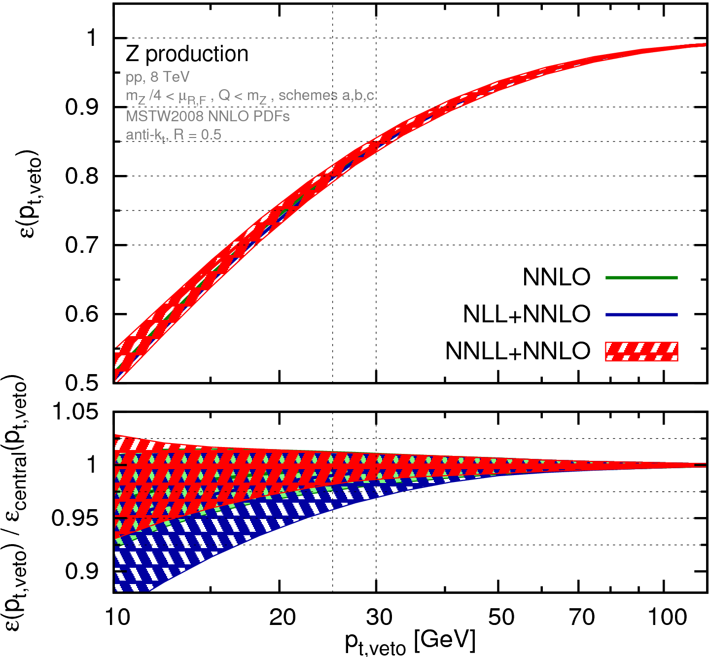
Figure 27: Jet-veto efficiency for $Z$-boson production at the 8 TeV LHC. The lower panel shows distributions normalised to the NNLL+NNLO central value. Figure from Ref. [271].

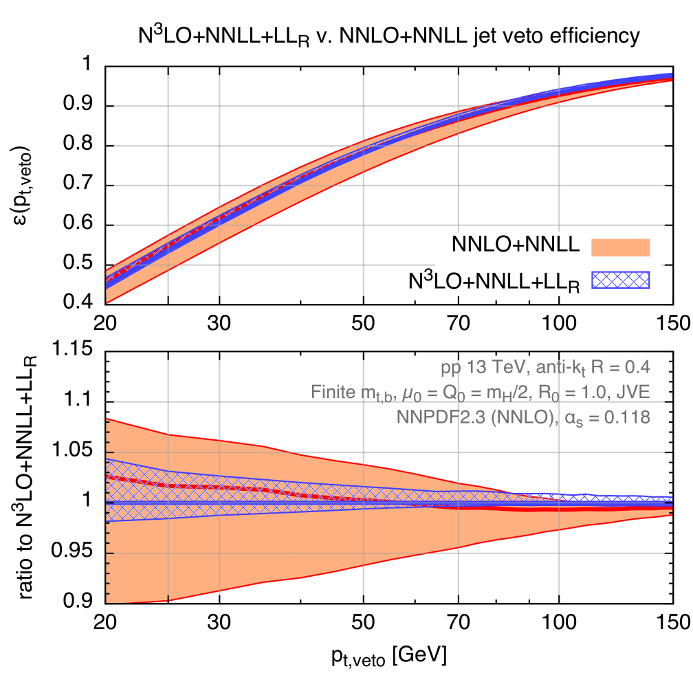
Figure 28: N³LO+NNLL+LL_R, best prediction for jet veto efficiency at 13 TeV LHC compared to NNLO+NNLL. Figure from Ref. [272].

In Ref. [271] such resummation has been performed at the next-to-next-to-leading-logarithmic (NNLL) accuracy, for the Higgs and $Z$ boson production, and it has been matched to the NNLO results [273, 264, 274, 275]. In Ref. [272], the jet-veto resummed prediction for the Higgs production in gluon fusion has been matched to the recent N³LO calculation [276] and further extended by including small-$R$ resummation [165] up to LL and finite mass effects up to NLO [277].

The above studies focused on computing the quantity called the jet veto efficiency, defined as [278]

$$\epsilon(p_{T}^{\text{veto}})\equiv\frac{\Sigma(p_{T}^{\text{veto}})}{\sigma_{\text{tot}}}\qquad\text{and}\qquad\Sigma(p_{T}^{\text{veto}})=\sum_{N}\int d\Phi_{N}\frac{d\sigma_{N}}{d\Phi_{N}}\Theta(p_{T}^{\text{veto}}-p_{T,j1}(p_{1},\ldots,p_{N}))\,,$$ (4.19)

where $\sigma_{\text{tot}}$ is the total cross section, $p_{T,j1}$ is the transverse momentum of the hardest jet and $d\sigma_{N}$ is a partonic cross section for the production of the Higgs or $Z$ boson in association with $N$ partons.

The NNLL resummation in $p_{T}^{\text{veto}}$ was performed using the Caesar approach [279] and, up to the NLL accuracy, it could be incorporated via a Sudakov form factor [278]. At that order, all emissions can be treated as independent and one can assume that each emitted parton forms a separate jet. At the NNLL order, these assumptions do not hold and the resummation formula needs to be supplemented with terms accounting for correlations between two emissions, as well as corrections arising when two gluons are clustered into a single jet [271]. These corrections, together with the previously known NNLL pieces complete the NNLL result for the jet veto resummation.

The most precise, currently available predictions for the jet veto efficiencies for the $Z$ boson production [271] at the LHC with $\sqrt{s}=8\,\text{TeV}$ are shown in Fig. 28. Because the efficiency (4.19) is defined as a ratio of two cross sections, each of which has its own perturbative expansion, there exist several ways in which the quantity $\epsilon$ can be computed. All of them are equivalent up to the order NNLO and differ only by terms ${{\cal O}\left({\alpha_{s}}^{3}\right)}$.

Refs. [278, 271] adopted an envelope-based method to asses uncertainties of the resummed predictions. The motivation behind using envelopes is to avoid double counting between uncertainties coming from various sources. Hence, at most one source is probed at a time. In practice, one takes an envelope from the scale variation band in one resummation scheme and the central values of the other schemes [278].

The above method of assessing the uncertainties has been further developed and is now called the jet-veto efficiency (JVE) method [280]. The efficiencies are effectively ratios of $N$-jet exclusive to $N$-jet inclusive cross sections and their uncertainties are driven by the Sudakov suppression terms. Therefore, one can treat the uncertainties in the efficiencies and in the inclusive cross sections as largely uncorrelated since the latter contains in addition uncertainties from genuine higher order corrections. In the JVE method, the uncertainties of efficiencies are obtained as envelopes and are combined with the uncertainties from inclusive cross sections using the above assumption.

As we see in Fig. 28, in the $Z$ boson case, the uncertainties of the NNLL+NNLO result are visibly smaller than those of NLL+NNLO and very similar to the fixed order NNLO result. In the case of Higgs production (see Ref. [271] for analogous figure), the uncertainties of the NNLL+NNLO result are much smaller than those of the NNLO result but comparable to NLL+NNLO.

The state-of-the-art predictions of the jet-veto efficiency for the Higgs boson production in gluon fusion is shown in Fig. 28. The previous results at NNLO+NNLL are compared to the updated prediction which includes the complete order N³LO as well as the small-$R$ and finite-mass effects. The central value of the renormalization and factorization scales was set at $\mu_{0}=m_{H}/2$. We see that inclusion of the exact, three-loop result has a very strong effect on the scale uncertainties, which are reduced from 10% to less than 5%, but change in the central value is small. We note that the JVE prescription for estimation of the uncertainties has been modified in Ref. [272] by limiting the number of schemes used for envelope determination. As further discussed in Ref. [272], while the N³LO corrections are included, the effects of jet-veto resummation are very small, both in terms of the central value and the uncertainties. Also the finite-mass and small-$R$ effects are at a per-cent level.

Resummation of the jet-veto logarithms for the Higgs production cross sections has been also performed within SCET at the NNLL accuracy [281], as well as at a very good approximation to the N³LL order, dubbed N³LL_p [282]. In both cases, the results were matched to the fixed order at the NNLO accuracy. Unlike in Refs. [278, 271, 272], which resum logarithms in the jet-veto efficiency, c.f. Eq. (4.19), here the resummation is performed directly for the Higgs cross section. A clear pattern of uncertainty reduction is observed when going from NLL, through NNLL to the N³LL_p accuracy. The components not captured by the N³LL_p result, one of which is the ${{\cal O}\left({\alpha_{s}}^{3}\right)}$ correction coming from the jet radius logarithms, were estimated to be small. This was partially confirmed by a direct calculation in Ref. [283].

The jet-veto results from SCET are compatible with those obtained within the standard QCD approach. In particular, the $\ln R$ dependence, known up ${{\cal O}\left({\alpha_{s}}^{2}\right)}$, agrees between the two frameworks [282]. Those jet-radius terms turn out to lead to sizable uncertainties for small-$R$ jets, which provides further motivation for efforts to resum such corrections, c.f. Section 4.2.

Because the Caesar-based results were obtained for the jet veto efficiencies while the SCET calculations were performed for the cross sections, direct comparisons of the two is not unambiguous. However, one can conclude that the numerical results from the two frameworks are compatible, within theoretical uncertainties, but the differences, which come from incomplete ${{\cal O}\left({\alpha_{s}}^{3}\right)}$ terms, are not negligible, c.f. Fig. 12 of Ref. [282].

Another motivation for the jet veto procedure comes from searches for the anomalous triple gauge boson couplings (aTGCs). These searches are performed by looking at deviations in the cross sections for various combinations of dibosons, like $WZ$, $WW$, $WH$, etc. As shown in Ref. [284], deviations in differential cross sections are observed only if there is a significant momentum transfer through the triple gauge boson vertex. This is achieved in configurations with the two bosons going back to back, as depicted in Fig. 30 (a). If one allows for a jet radiation produced in association with the diboson pair, the amount of transverse momentum flowing through the triple gauge boson vertex is reduced, as the hard jet will typically recoil against the system of the collinear boson pair, c.f. Fig. 30 (b). Another way in which jets reduce sensitivity to aTGCs is via configurations depicted in Fig. 30 (c), where the bosons do not originate from a single vertex but each of them is radiated separately from a quark line. Triggering on large transverse momentum of one of the boson (or its decay products) favours configuration in which the other boson is soft or collinear to the energetic quark. Such diagrams are enhanced by the logarithmic factor $\ln\big{(}{p_{T,\text{jet}}^{2}}/{m_{V}^{2}}\big{)}$ and, since they do not involve the triple boson vertex, sensitivity to the anomalous coupling effects is decreased.

By imposing a veto on the jet radiation, one can enhance configurations of the type shown in Fig. 30 (a), in which the two bosons are produced back-to-back. Then, by requiring each of them to be sufficiently hard, large transverse momentum flow through the triple gauge boson vertex is assured.

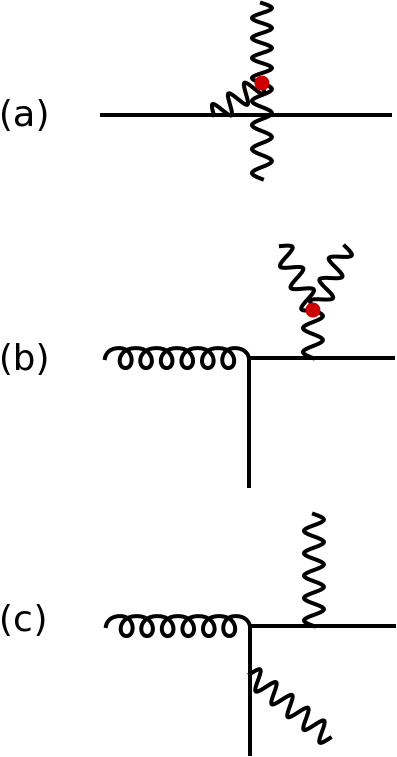
Figure 29: Different configurations appearing in diboson process, $VV$: (a) back-to-back production, (b) $V$ recoiling against a jet, (c) soft or collinear $V$ emission from a quark.

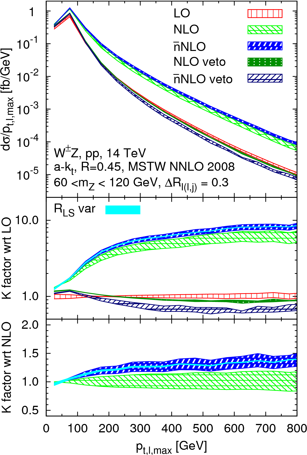
Figure 30: Differential cross sections and K factors for the $p_{T}$ of the hardest lepton in $WZ$ production at the LHC at $\sqrt{s}=14\,\text{TeV}$ with an without jet veto. Figure from Ref. [245].

These effects have been studied in Refs. [245, 246, 285] and Fig. 30 shows an example for the $WZ$ production. The distributions of the hardest lepton transverse momentum were computed with Vbfnlo [205, 206] together with the LoopSim [243, 244] package, which allows one to account for the dominant part of the NNLO corrections at high transverse momentum of the leading lepton, $p_{T,l,\max}$. The renormalization and factorization scales were set to $\mu_{F,R}=\frac{1}{2}\sum p_{T,\text{partons}}+\frac{1}{2}\sqrt{p_{T,W}^{2}+m_{W}^{2}}+\frac{1}{2}\sqrt{p_{T,Z}^{2}+m_{Z}^{2}}$ and the bands correspond to varying $\mu_{F}=\mu_{R}$ by factors 1/2 and 2 around the central value. The cyan solid bands give the uncertainty related to the $R_{\text{LS}}$ parameter of LoopSim, which is varied between 0.5 and 1.5. As we see, the factorization and renormalisation scale uncertainties dominate above 100 GeV.

The large correction from LO to NLO for the inclusive sample (i.e. with no restriction on jet radiation) comes from the configurations of Fig. 30 (c), with soft and collinear emissions of the vector boson. We see that the approximate NNLO correction, labeled as $\bar{n}$NLO, is still significant for the inclusive $WZ$ production, reaching up to 30% of the NLO result at high $p_{T}$.

The situation is very different if the jet veto, forbidding the radiation with $p_{T,\text{jet}}>50\,\text{GeV}$, is imposed. This leads to suppression of the configurations shown in Figs. 30 (b) and (c) and one is left with contributions from events with the two hard vector bosons recoiling against each other.

Fig. 30 shows the generic problem of the standard jet veto procedure. At NLO, the distribution seems to be very well behaved, with small corrections with respect to LO and with the reduced scale uncertainty. The $\bar{n}$NLO result, however, reveals further, significant corrections and the corresponding uncertainty band is broader than that of NLO. This effect comes from Sudakov-type logarithms introduced by the veto procedure, which forbid radiation in certain regions of phase space. These logarithms bring negative corrections to the cross section at high $p_{T}$. Hence, the NLO/LO and $\bar{n}$NLO/LO K-factors rise a little, but as $p_{T,l,\max}$ increases, the restriction for additional radiation leads to suppression and eventually fairly rapid drop of the K-factors. Of course, the full NNLO correction will also receive contribution from, potentially non-negligible constant term of the two-loop diagrams. However, the approximate $\bar{n}$NLO result for the vetoed case gives already an indications what happens at ${{\cal O}\left(\alpha_{\text{\sc ew}}^{2}{\alpha_{s}}^{2}\right)}$. Moreover, as shown in Fig. 30, as well as other distributions discussed in Refs. [245, 246, 285], it demonstrates that the small scale uncertainties of many of the NLO results with a jet veto are to a large extent accidental, as the corresponding uncertainty at $\bar{n}$NLO comes out larger than that of NLO. The misleadingly small scale uncertainties of the vetoed events come from cancellations between large perturbative NLO corrections and terms involving logarithms of the veto scale.

The problem of accidental cancellation occurring in events with jet vetoes has been carefully addressed in Ref. [286], where a method superior to a simple scale variation in exclusive, fixed-order predictions has been proposed. The exclusive, $N$-jet cross section can be defined as a difference of the inclusive cross sections: $\sigma_{N}=\sigma_{\geq N}-\sigma_{\geq N+1}$. By varying a scale in the exclusive cross section, we implicitly assume 100% correlation between the uncertainties of the two inclusive cross sections. However, there is a priori no reason for that assumption.

An inclusive, $N$-jet cross section is sensitive to the minimal jet transverse momentum, $p_{T}^{\text{cut}}$, through the logarithms $L=\ln\left(p_{T}^{\text{cut}}/Q\right)$, where $Q$ is the hard scale of the process, e.g. mass of the Higgs boson. Powers of such logarithms multiply various powers of ${\alpha_{s}}$. For experimentally relevant values of the transverse momenta, these logarithms are large and the variation of $Q$, as well as the renormalization scale in ${\alpha_{s}}$, provides a realistic assessment of the uncertainty due to missing higher orders. However, in the difference of the two inclusive cross sections, which gives the exclusive cross section $\sigma_{N}$, the coefficients multiplying the powers of ${\alpha_{s}}$ vanish for certain value of $L$. This is a cancellation between the genuine higher order corrections and the terms generated by the veto procedure and it turns out to happen for the values of $p_{T}^{\text{cut}}$ that are currently used in analyses of the LHC data.

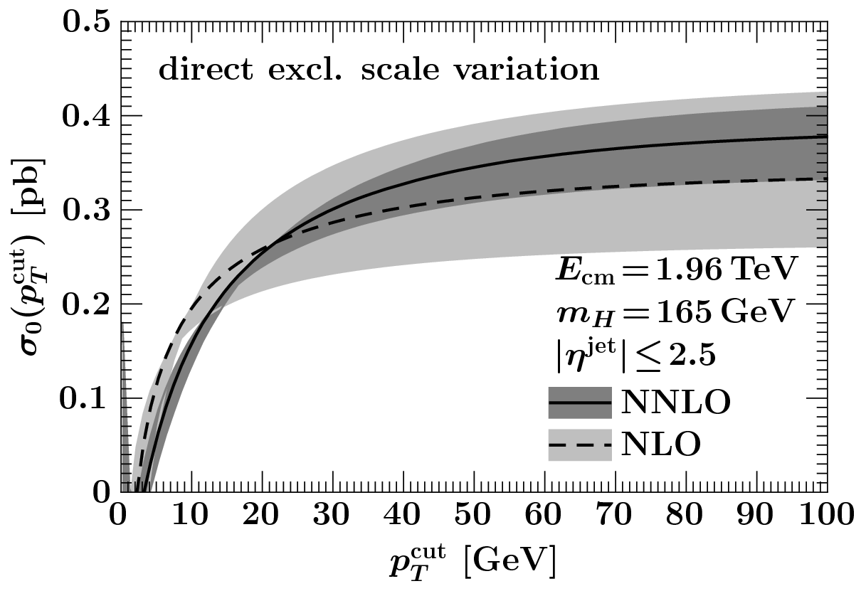
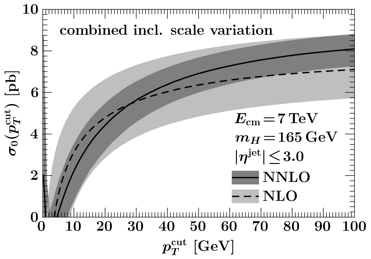
Figure 31: Scale variation uncertainties for exclusive $gg\to H+0\,\text{jets}$ production at NLO and NNLO. On the left, the bands are obtained by the standard scale variation in the exclusive cross section, while on the right, by combining the uncertainties of inclusive 0- and 1-jet cross sections in quadrature. Figure from Ref. [286].

Consider a simple case of the $0$-jet inclusive production. The inclusive cross section reads: $\sigma_{\geq 0}=\sigma_{0}(p_{T}^{\text{cut}})+\sigma_{\geq 1}(p_{T}^{\text{cut}})$. Since the $0$-jet inclusive cross section cannot depend on $p_{T}^{\text{cut}}$, additional perturbative uncertainty induced by the cut (through the logarithms mentioned above), $\Delta_{\text{cut}}^{2}$, must be 100% anti-correlated between $\sigma_{0}$ and $\sigma_{\geq 1}$. Because the veto-induced terms are large, it is justified to assume that $\Delta_{\geq 1}^{2}\simeq\Delta_{\text{cut}}^{2}$, i.e. the uncertainty coming from the veto is equal to the total uncertainty of the $1$-jet inclusive cross section. The uncertainty of the $0$-jet inclusive cross section, $\Delta_{\geq 0}^{2}$, is independent of $\Delta_{\text{cut}}^{2}$, it is therefore also independent of $\Delta_{\geq 1}^{2}$. From the above, it follows that the uncertainty of the $0$-jet exclusive cross section, which is what we want to calculate, is, to a good approximation, given by $\Delta_{\geq 0}^{2}+\Delta_{\geq 1}^{2}$. Hence, contrary to the standard procedure, in this approach, the $N$ and $N+1$-inclusive cross sections are assumed to be 100% uncorrelated.

As shown in Fig. 31 (left), the standard procedure of scale variation in the exclusive cross section for the Higgs production in gluon fusion gives misleadingly small uncertainties at NLO. Hence, the NLO band does not cover the NNLO distribution, which means that the uncertainty due to missing higher order terms is not estimated correctly. On the contrary, the procedure of combining the uncertainties of the inclusive cross sections, described above, gives a much more realistic assessment of the theoretical errors, as shown in Fig. 31 (right).

Another approach to the problem of the large logarithmic corrections associated with setting a sharp cut on jet radiation is to modify the veto procedure such that the logarithmic enhancement is reduced. Ref. [285] introduced the so-called dynamical jet veto, where, instead of using a fixed $p_{T}$ cut, the jet veto is applied on the event-by-event basis with help of the variables

$$x_{\text{jet}}=\frac{\sum_{\text{jets}}E_{T,i}}{\sum_{\text{jets}}E_{T,i}+\sum_{V}E_{T,i}}\,,\qquad\qquad\qquad x_{V}=\frac{E_{T,V}}{\sum_{\text{jets}}E_{T,i}+\sum_{V}E_{T,i}}\,.$$ (4.20)

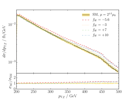
Figure 32: Differential transverse momentum distribution of the $Z$ boson in $WZ$ production at NLO for different values of the anomalous coupling $f_{W}$ without (left) and with (right) a dynamical jet veto. Figure from Ref. [285].

As shown in Ref. [285], for the diboson production processes, the sensitivity to aTGCs lies in the region of $x_{\text{jet}}\lesssim 0.2-0.3$. At the same time, most of the events have $x_{\text{jet}}\simeq 0.4-0.5$. Hence, vetoing the events with $x_{\text{jet}}>0.2$ will lead to a significant increase of the sensitivity to aTGC. This is illustrated in Fig. 32 which shows $p_{T,Z}$ distributions obtained with different values of the anomalous coupling $f_{W}$ (including the SM case of $f_{W}=0$). On the left hand side, no veto was used and we see that the sensitivity to $f_{W}$ variation is limited. The right plot shows the effect of applying the dynamical veto procedure. We see that sensitivity to the $f_{W}$ values increases significantly, especially at high $p_{T}$. At the same time, the uncertainty band from scale variation (shown for SM only) decreases only moderately unlike in the case of fixed-$p_{T}$ veto discussed earlier in the context of Fig. 30, where it was nearly vanishing at NLO. Stability of the result with the dynamical veto indicates that the effect of Sudakov logarithms is mild.

4.5 Forward jets

The main features of the kinematics of jet processes in hadron-hadron collisions can be understood by analysing a simple $2\to 2$ partonic scattering. The relation between the rapidities and the transverse momenta of the outgoing partons (our proxies for jets) and the fraction of energies carried by the incoming partons corresponds to Eq. (3.25) introduced in Section 3.4.1.

Most of the jets measured at the LHC are produced in the central rapidity region, $y_{\text{jet}}\sim 0$, hence, the energy fractions of the incoming partons are comparable, and typically larger than $10^{-2}$. Therefore, the central dijet production corresponds to the case $x_{1}\sim x_{2}\lesssim 1$. This region of phase-space is amenable to standard treatment in the framework of the collinear factorization discussed in Section 3.1, with PDFs evolved according to DGLAP equations and combined with the collinear matrix elements.

The above canonical framework is expected to break down when more extreme corners of phase-space are probed. Those can be reached in processes with forward jets. In the case of dijet production, we can have both of the jets going forward, one forward and one central jet, or one jet going in the forward and the other in the backward direction. The forward-forward case corresponds to $x_{1}\sim 1$, $x_{2}\ll 1$, the forward-central to $x_{1}\sim 1$, $x_{2}\lesssim 1$ and the forward-backward to $x_{1}\sim 1$, $x_{2}\sim 1$.

Each of this regions poses challenges to the standard approaches based on the collinear factorization. In the forward-forward case, one of the incoming hadrons is probed at very low momentum fractions, which leads to appearance of large logarithms, $\ln(1/x)$, from initial state emissions. These logarithms should be resummed, which can be achieved by means of the BFKL [287, 288, 289] or CCFM [290, 291, 292] equations. Those formalisms go beyond simple collinear factorization, as they result in parton distributions which are unintegrated in the transverse momentum and therefore are only compatible with some form of the TMD factorization, c.f. Section 3.3.

Similar issues arise in the case of the forward-central dijet production, where, in addition, a potentially large rapidity gap between the two jets opens a phase for addition BFKL-type emissions from the final state. Finally, in the case of the forward-backward dijet production, rapidity separation between the jets is even larger and the process falls into the category of the so-called Mueller-Navelet (MN) jets [293]. In this case, the use of collinear factorization is justified as both $x_{1}$ and $x_{2}$ are large, but one needs to include BFKL resummation of the final state, wide-angle radiation [294, 295].

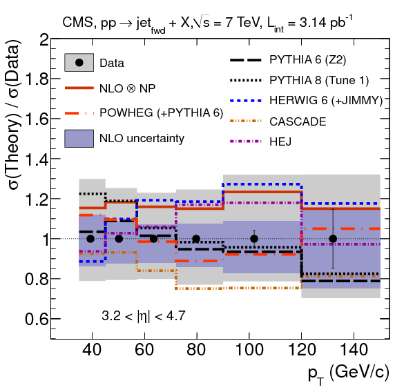
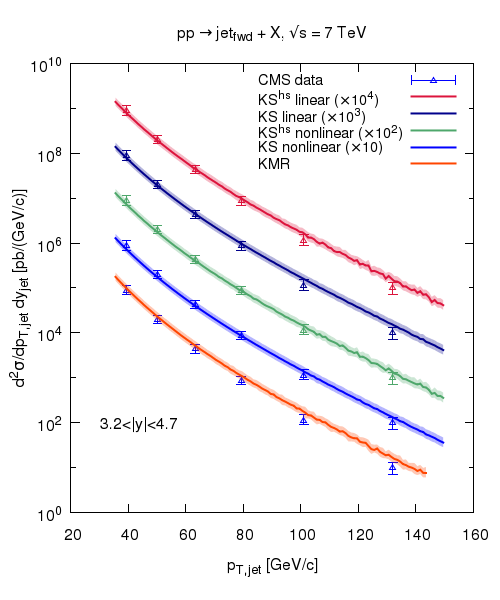
Figure 33: Single inclusive production of forward jets. Comparison between CMS data and predictions from a range of theoretical approaches both within the collinear (left: Herwig, Pythia, Hej) and the high energy factorization frameworks (left: Cascade, right: HEF with KS and KMR gluons). Figures from Refs. [8] and [296], respectively.

In the following, we shall briefly describe the existing theoretical approaches to the forward jet processes and confront them with experimental data from the LHC.

The Cascade [297] is a MC event generator based on the CCFM evolution equation [290, 291, 292]. The latter resummes both the $\ln\left(1/x\right)$ and $\ln Q^{2}$ terms, to all orders in the leading logarithmic approximation, providing appropriate unintegrated gluon distributions. In Cascade, the CFFM equation is used for probabilistic, backward generation of gluon radiation, starting from the hard scattering process described by an off-shell matrix element. This procedure is, in principle, compatible with the high energy factorization [122, 123]. Final-state parton shower and hadronization are subsequently added via an interface to Pythia. The framework has been used to fit parameters of the unintegrated gluon distributions to the HERA data [297].

The hybrid high energy factorization framework, introduced in Section 3.4.2 can be directly employed to study forward dijets by integrating the formula (3.28). The calculations can be performed with the public codes of Refs. [298, 296, 299]. Here, one can use a range of unintegrated gluons fitted to DIS data, like those obtained in Refs. [127, 300]. A generalized version of HEF, the improved TMD factorization, c.f. Section 3.4.3, is in principle better, as long as one is able to determine multiple gluon distributions entering Eq. (3.4.3).

The high energy jets (HEJ) framework [294, 295, 301], implemented in the Hejprogram, provides all-order resummation of the leading logarithmic contributions to the wide-angle, hard QCD radiation. These contributions are dominant in the high energy limit, where all invariants involving the outgoing partons are large and their transverse momenta are fixed. In this limit, the scattering amplitudes factorize into rapidity ordered pieces which allows for efficient evaluation of the matrix element. This is analogous to what happens in the collinear limit, where multi-parton cross sections factorize, which in turn is a basis for construction of a parton shower. The HEJ approach can be thought of as being complementary to the parton shower and the two have been indeed combined [302] providing simultaneous description of the large- and small-angle, multi-particle emissions. Both pure $n$-jet processes, with $n\geq 2$, as well as dijets in association with a vector boson or the Higgs boson [303], are implemented in the Hejprogram. The approach is relevant for production of the central-forward and Mueller-Navelet jets, as it capable of filling up the large rapidity gap between the jets with gluon radiation.

BFKL-based approaches are also used to study Mueller-Navelet jets. Differential cross sections are calculated in the framework of the high energy factorization with the unintegrated gluons obtained from ordinary collinear PDFs convoluted with jet vertices, currently known at the next-to-leading-logarithmic (NLL) accuracy [304, 305]. The off-shell matrix elements are provided by the BFKL kernel, also known up to NLL. As discussed in Ref. [306], predictions for broad class of observables, most notably the moments of distributions of the azimuthal distance between the jets, are different in this framework, as compared to the standard NLO. The MN jets are therefore very suitable for searches of BFKL dynamics. For further important studies of the Mueller-Navelet jets see Refs. [307, 308, 309, 310, 311].

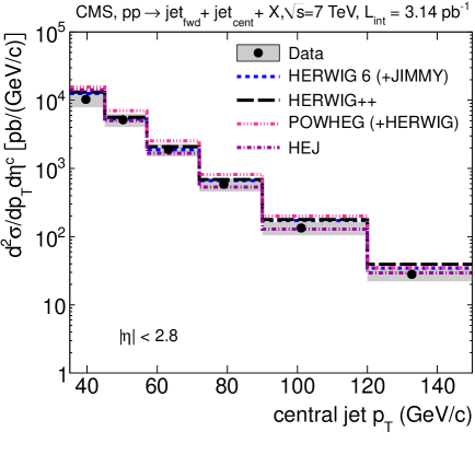
Figure 34: Differential cross sections as a function of the central (left) and the forward (right) jet $p_{T}$ in the central-forward dijet production as measured by CMS in comparison with various theoretical predictions, all within the framework of collinear factorization. Figure from Ref. [8].

The LHC experiments have performed many interesting measurements with forward jets. The inclusive jets and dijets production in the forward region have been studied both by ATLAS and CMS. In Fig. 33, we show a comparison between the CMS data [8] for the jet’s transverse momentum distributions in the single inclusive production, and various theoretical calculations. Overall agreement within 20% experimental uncertainty band is found for most predictions. We note that good description is obtained both within the collinear factorization framework (NLO, Powheg), as well within the hybrid high energy factorization with the KS [127, 312] or KMR [300] gluons.

Production of the central-forward dijets, with rapidities, $|y|<2.8$ and $3.2<|y|<4.7$, respectively, was also studied by CMS. As this measurement is less inclusive than the single jet production, it is more challenging to describe theoretically. Indeed, as found in Ref. [8], the results from Pythia, Herwig and Cascade show various levels of agreement with the data, from 30% to a factor of 2, depending on the distribution ($p_{T}$ of the central or the forward jet) as well as a specific tune of the Monte Carlo. The results from Herwig, Powheg and Hejdescribe the data better, within 30-50%, as shown in Fig. 34.

Of particular interest is a distribution of the azimuthal separation between two leading jets, $\Delta\phi$, the so-called azimuthal decorrelation. In the framework of the collinear factorization, azimuthal decorrelation is sensitive to the initial state radiation (ISR), which boosts the dijet system in the transverse direction. In the language of the high energy factorization, this ISR radiation is what builds up the non-zero $k_{T}$ of the incoming gluon and it is effectively resumed in the unintegrated gluon TMDs.

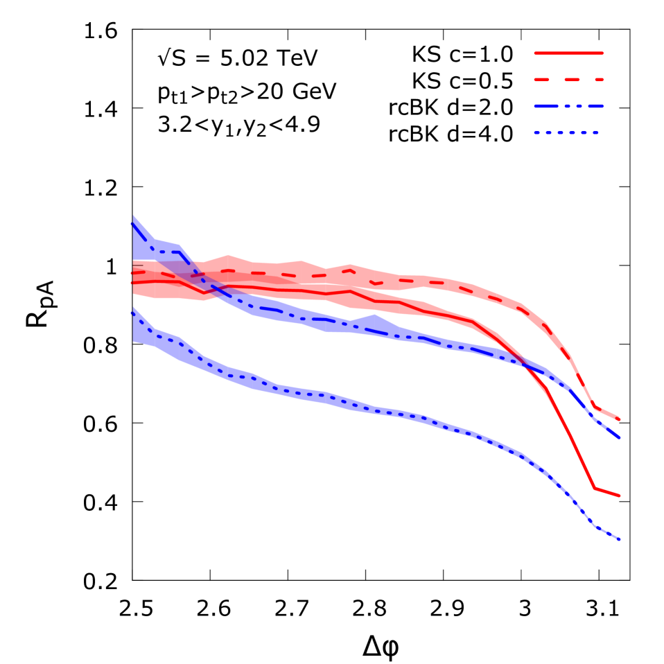
Figure 35: Nuclear modification ratios for azimuthal decorrelations in the forward-forward dijet production. The predictions were obtained within HEF. See text for details. Figure from Ref. [129].

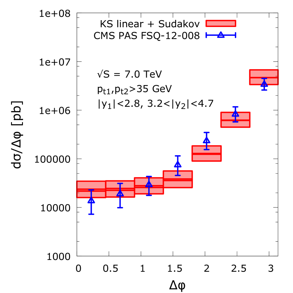
Figure 36: Azimuthal decorrelation in central-forward dijet production at the LHC, 7 TeV, compared to theoretical predictions obtained within high energy factorization. Figure from Ref. [130].

According to Eq. (3.27), the region of $\Delta\phi\sim\pi$, which corresponds to the nearly back-to-back dijet configurations, probes the gluon distributions at very low transverse momenta. If, at the same time, the two jets are produced in the forward direction, most of the contribution to the cross section comes from the low-$x$ region. The corner of phase space with low $x$ and low $k_{T}$ is a domain of a non-linear QCD evolution and the related phenomenon of saturation [313, 314, 315]. Hence, azimuthal decorrelation in the forward-forward dijet production is a very promising observable to test this extreme regime of QCD.

Because the saturation scale is proportional to $A^{1/3}$, where $A$ is the atomic number of the target, the nonlinear regime of the gluon density is reached earlier in heavy ions. By forming a ratio of the azimuthal decorrelations in the proton-lead and proton-proton collisions, we are able to obtain a robust signature of gluon saturation in the forward dijet production. Fig. 36 shows such ratios, $R_{pA}=1/A\,(d\sigma^{pA}/d\Delta\phi)/(d\sigma^{pp}/d\Delta\phi)$, for several scenarios with different unintegrated gluons (KS [127] or rcBK [316]) and different parameters entering the modeling of the transition from the proton, whose unintegrated PDFs were fitted to HERA data, to lead. We see that, regardless of the model, strong suppression of the $R_{pA}$ ratio is predicted in the region $\Delta\phi\sim\pi$.

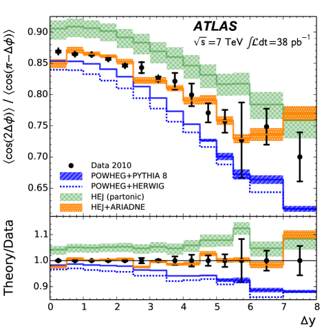
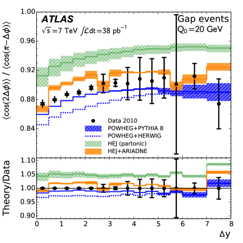
Figure 37: Ratios of the second to the first moment of the azimuthal decorrelation distribution for the production of dijets separated by the rapidity distance $\Delta y$. The left plot corresponds to inclusive dijet production whereas on the right hand side no jet activity with $p_{T}$ above 20 GeV is allowed in the gap between the two leading jets. Figures from Ref. [317].

Azimuthal decorrelation has been studied so far by CMS in the central-forward dijet production in Ref. [318]. There, the data were compared to various theoretical predictions. The latter were obtained with the standard Monte Carlo programs, where decorrelation is generated by the parton shower, superimposed on top of the $2\to 2$ hard scattering. The final-state partons are then hadronized and the predictions include in addition contributions from the underlying event and multi-parton interactions. The MC models tend to describe the data within systematic uncertainties.

In Fig. 36, the same data are compared to predictions from the HEF formalism, with the KS gluon supplemented by the hard scale dependence by means of reweighting the gluon distribution with the Sudakov form factor [130]. The predictions describe the CMS data comparably to the LL MCs studied in Ref. [318]. This is an important observation as the two frameworks, HEF and LL MCs, are constructed with very different sets of approximations. In HEF, the transverse momentum of the dijet pair, $k_{T}$, is generated as a result of evolution of the unintegrated gluon distribution function, and its value enters the off-shell matrix element for the $2\to 2$ process. However, the LL MCs are built in the framework of the collinear factorization, hence the incoming partons have zero transverse momenta. In this case, the $k_{T}$ of the dijet pair comes from the subsequent, initial-state radiation (ISR), which is part of the hard process and not the parton distributions. This radiation, generated in the parton shower approximation, effectively provides parts of contributions coming from higher multiplicities. At the end, however, the two frameworks, albeit through different means, realize the same task of generation of the ISR emissions, hence they are supposed to grasp the same physics. Therefore, it is not surprising that the same features are seen in the distributions obtained in HEF and in the collinear factorization supplemented with a parton shower. What is non-trivial in the context of Fig. 36 (and its analogue, Fig. 4 of Ref. [318]) is that the two frameworks provide predictions which are quantitatively consistent.

It is also interesting to analyse the azimuthal decorrelation as a function of the rapidity separation between the jets in the dijet system. When this separation is large, patterns of radiation are expected to be very different in the DGLAP- and BFKL-based approaches, as in the former, the emissions are ordered in the transverse momentum while in the latter, in rapidity. The normalized cross section, $1/\sigma\,d\sigma/d\Delta\phi$, can be expanded in Fourier series and the corresponding coefficients are given by the moments $\langle\cos\left(n(\pi-\Delta\phi)\right)\rangle$. The ratios of the second and the first moment are shown in Fig. 37 for the inclusive case of dijet production (left) and for the case where the hard radiation is forbidden in the space between the two leading jets (right). Here, none of the jets is explicitly required to be forward. However, when the rapidity separation, $\Delta y$, is sizable, one or both are likely to be produced at large (positive or negative) rapidities. We see that the inclusive case is well described by Hejwith the Ariadneparton shower, while Powheg fails to describe the data. However, with the gap requirement, hence forbidding radiation between the jets, both Hej+Ariadneand Powheg predictions lie close to the experimental points. This can be interpreted as an indication that, in the inclusive case shown in Fig. 37 (left), the wide-angle, multi-jet radiation, created abundantly in the space between two well-separated jets, is modeled better by the approach based on BFKL evolution.

A related study has been performed by CMS [319], where a similar ratio is well described by analytic calculation within NLL BFKL [306]. However, both in the ATLAS [317] and in the CMS [319] studies, some aspects of the data are also well reproduced by DGLAP-based approaches hence, no firm conclusion can be drawn at this point. A detailed analysis of dijet production with a veto on central jet activity has been also published by ATLAS in Ref. [320], where the predictions from Hejand Powheg are extensively tested against the data.

We conclude by noting that the range of theoretical frameworks used to describe the forward jet production, and briefly mentioned above, differ considerably both in the grasped aspects of physics of these class of processes, as well as in the level of theoretical sophistication. Many of them are of LO or LO+LL accuracy and, in some cases, jets are approximated only by a single, leading particle. This certainly leaves a room for improvements, which, amongst other things, would lead to more realistic modeling of the final states that could be in turn analysed with the fully general jet finding techniques discussed in Section 2.

5 Summary and outlook

Jets are omnipresent at hadron colliders and physics of jets is by now a well-grounded and highly developed area of research. That allows for precise and quantitative discussion and this review tried to make an account of the concepts and results that are vital to studies of jet processes.

The LHC opened a new chapter in jet physics through the exclusive use of the infrared and collinear-safe jet definitions by all its experiments. That laid a foundation for accurate measurements and provided strong motivation for theoretical efforts aiming at calculating the higher order corrections to jet processes.

We have discussed some of the advances in controlling jets and understanding their properties. We saw that individual jets produced in hadron-hadron collisions differ in many ways and that diversity should be turned to our advantage. It is therefore advisable to choose jet definitions based on specificities of the analyses one is interested to perform, such as: expected backgrounds, final state cuts and potential contamination from incoherent radiation. Recent years have seen many developments in the area of jet-based analyses methods, especially those related to the substructure techniques, treated only briefly in this review. These results allow for even broader use of jets in precise test of the Standard Model and searches for new physics. A truly impressive progress has been also made in calculating the perturbative predictions for the processes with jet production. We have discussed the highest precision, fixed-order, results, which, in the recent years, have been pushed in many cases to the NNLO accuracy or were supplemented by electro-weak corrections. We have also extensively elaborated on techniques for matching the NLO and the NNLO results to a parton shower or merging the NLO results with different multiplicities. Those methods allow one to achieve predictions of the highest accuracy simultaneously for the inclusive and for a range of exclusive observables. All of the above advances went hand-in-hand with proposals of genuinely new calculational techniques and developments of efficient numerical tools.

The overall description of the experimental results for jet processes with the state-of-the-art theoretical predictions is very good. And it spans across numerous distributions and many orders of magnitude. However, there are still challenges and open questions that need to be addressed in order to push the precision of jet physics to the next level. Throughout the article, we have mentioned various sources that contribute to the theoretical and experimental uncertainties. The latter type consists of errors related to jet energy scale determination, luminosity measurements, unfolding and pileup. Theoretical uncertainties arise because of truncation of the perturbative series, limited accuracy of the parton showers, missing electroweak contributions, ambiguities in PDF determinations, including those related to the choice of factorization scheme, as well as potential factorization breaking effects. Many of the above uncertainties are being dealt with by systematically adding further terms with higher powers of the strong and electroweak couplings and by improving logarithmic accuracy of the showers and resummations.

Finally, jets are also produced in special regions of phase space or with strong cuts on their momenta. Such cases are very interesting, as they allow us to stretch tests of QCD to extreme corners. At the same time, they are challenging to model theoretically because of inapplicability of the standard frameworks. Therefore, we have discussed at length the delicate issue of factorization in jet production processes, reporting on the recent developments and indicating promising future directions. We have also pointed to potential measurements that could help to pin down the effects going beyond the standard description based on the collinear factorization and DGLAP evolution such as BFKL-type radiation and non-linear effects inside the initial-state hadrons.

References

- [1] S.D. Ellis, J. Huston, K. Hatakeyama, P. Loch, and M. Tonnesmann. Prog.Part.Nucl.Phys., 60:484–551, 2008.
- [2] T. Aaltonen et al. Phys. Rev., D78:052006, 2008. [Erratum: Phys. Rev.D79,119902(2009)].
- [3] Victor Mukhamedovich Abazov et al. Phys. Rev., D85:052006, 2012.
- [4] G. Aad et al. Eur.Phys.J., C71:1512, 2011.
- [5] Georges Aad et al. Phys.Rev., D86:014022, 2012.
- [6] Serguei Chatrchyan et al. Phys.Lett., B700:187–206, 2011.
- [7] Serguei Chatrchyan et al. Phys.Rev.Lett., 107:132001, 2011.
- [8] Serguei Chatrchyan et al. JHEP, 1206:036, 2012.
- [9] Serguei Chatrchyan et al. Phys.Rev., D87(11):112002, 2013.
- [10] Bogdan Malaescu and Pavel Starovoitov. Eur.Phys.J., C72:2041, 2012.
- [11] Juan Rojo. Int. J. Mod. Phys., A30:1546005, 2015.
- [12] Mikko Voutilainen. Int. J. Mod. Phys., A30(31):1546008, 2015.
- [13] Richard D. Ball et al. JHEP, 04:040, 2015.
- [14] Sayipjamal Dulat, Tie-Jiun Hou, Jun Gao, Marco Guzzi, Joey Huston, Pavel Nadolsky, Jon Pumplin, Carl Schmidt, Daniel Stump, and C. P. Yuan. Phys. Rev., D93(3):033006, 2016.
- [15] L. A. Harland-Lang, A. D. Martin, P. Motylinski, and R. S. Thorne. Eur. Phys. J., C75(5):204, 2015.
- [16] George Sterman. Acta Phys.Polon., B45:2205, 2014.
- [17] Francois Gelis, Edmond Iancu, Jamal Jalilian-Marian, and Raju Venugopalan. Ann. Rev. Nucl. Part. Sci., 60:463–489, 2010.
- [18] Mario Campanelli. Int. J. Mod. Phys., A30(31):1546006, 2015.
- [19] Serguei Chatrchyan et al. Phys.Rev., D87(11):114015, 2013.
- [20] Georges Aad et al. Phys. Rev., D91(5):052007, 2015.
- [21] Georges Aad et al. Phys. Lett., B705:294–312, 2013.
- [22] Vardan Khachatryan et al. Eur. Phys. J., C75(5):235, 2015.
- [23] Georges Aad et al. JHEP, 1502:153, 2015.
- [24] Georges Aad et al. Phys. Lett., B716:1–29, 2013.
- [25] Serguei Chatrchyan et al. Phys. Lett., B716:30–61, 2012.
- [26] Georges Aad et al. JHEP, 1301:029, 2013.
- [27] Georges Aad et al. Phys.Rev.Lett., 105:252303, 2010.
- [28] George F. Sterman and Steven Weinberg. Phys.Rev.Lett., 39:1436, 1977.
- [29] Gavin P. Salam. Eur.Phys.J., C67:637–686, 2010.
- [30] A. Altheimer et al. Eur. Phys. J., C74(3):2792, 2014.
- [31] D. Adams et al. Eur. Phys. J., C75(9):409, 2015.
- [32] Paolo Francavilla. Submitted to: Int. J. Mod. Phys., 2015.
- [33] Panagiotis Kokkas. Int. J. Mod. Phys., A30(31):1546004, 2015.
- [34] Matteo Cacciari. Int. J. Mod. Phys., A30(31):1546001, 2015.
- [35] N. Armesto, N. Borghini, S. Jeon, U. A. Wiedemann, S. Abreu, V. Akkelin, J. Alam, J. L. Albacete, A. Andronic, D. Antonov, et al. J. Phys., G35:054001, 2008.
- [36] Yacine Mehtar-Tani, Jose Guilherme Milhano, and Konrad Tywoniuk. Int. J. Mod. Phys., A28:1340013, 2013.
- [37] N. Armesto and E. Scomparin. Eur. Phys. J. Plus, 131(3):52, 2016.
- [38] Guang-You Qin and Xin-Nian Wang. Int. J. Mod. Phys., E24(11):1530014, 2015.
- [39] Matteo Cacciari, Juan Rojo, Gavin P. Salam, and Gregory Soyez. Eur. Phys. J., C71:1539, 2011.
- [40] S. Catani, Yuri L. Dokshitzer, M. H. Seymour, and B. R. Webber. Nucl. Phys., B406:187–224, 1993.
- [41] Stephen D. Ellis and Davison E. Soper. Phys. Rev., D48:3160–3166, 1993.
- [42] Yuri L. Dokshitzer, G. D. Leder, S. Moretti, and B. R. Webber. JHEP, 08:001, 1997.
- [43] M. Wobisch and T. Wengler. In Monte Carlo generators for HERA physics. Proceedings, Workshop, Hamburg, Germany, 1998-1999, 1998.
- [44] Gavin P. Salam and Gregory Soyez. JHEP, 0705:086, 2007.
- [45] Matteo Cacciari and Gavin P. Salam. Phys. Lett., B641:57–61, 2006.
- [46] Matteo Cacciari, Gavin P. Salam, and Gregory Soyez. JHEP, 04:063, 2008.
- [47] T. Kinoshita. J. Math. Phys., 3:650–677, 1962.
- [48] T. D. Lee and M. Nauenberg. Phys. Rev., 133:B1549–B1562, 1964.
- [49] Matteo Cacciari, Gavin P. Salam, and Gregory Soyez. Eur. Phys. J., C72:1896, 2012.
- [50] Paloma Quiroga-Arias and Sebastian Sapeta. Int. J. Mod. Phys., A28:1350087, 2013.
- [51] Leandro G. Almeida, Seung J. Lee, Gilad Perez, Ilmo Sung, and Joseph Virzi. Phys. Rev., D79:074012, 2009.
- [52] Matteo Cacciari, Gavin P. Salam, and Gregory Soyez. JHEP, 0804:005, 2008.
- [53] Sebastian Sapeta and Qi Cheng Zhang. JHEP, 06:038, 2011.
- [54] Torbjorn Sjostrand, Stephen Mrenna, and Peter Z. Skands. JHEP, 05:026, 2006.
- [55] Michael H. Seymour. Z. Phys., C62:127–138, 1994.
- [56] J. M. Butterworth, B. E. Cox, and Jeffrey R. Forshaw. Phys. Rev., D65:096014, 2002.
- [57] J. M. Butterworth, John R. Ellis, and A. R. Raklev. JHEP, 05:033, 2007.
- [58] Jonathan M. Butterworth, Adam R. Davison, Mathieu Rubin, and Gavin P. Salam. Phys. Rev. Lett., 100:242001, 2008.
- [59] Mathieu Rubin. JHEP, 05:005, 2010.
- [60] Mrinal Dasgupta, Alessandro Fregoso, Simone Marzani, and Gavin P. Salam. JHEP, 09:029, 2013.
- [61] Stephen D. Ellis, Christopher K. Vermilion, and Jonathan R. Walsh. Phys. Rev., D80:051501, 2009.
- [62] Stephen D. Ellis, Christopher K. Vermilion, and Jonathan R. Walsh. Phys. Rev., D81:094023, 2010.
- [63] David Krohn, Jesse Thaler, and Lian-Tao Wang. JHEP, 02:084, 2010.
- [64] Jesse Thaler and Ken Van Tilburg. JHEP, 03:015, 2011.
- [65] Jesse Thaler and Ken Van Tilburg. JHEP, 02:093, 2012.
- [66] Davison E. Soper and Michael Spannowsky. JHEP, 08:029, 2010.
- [67] Ilya Feige, Matthew D. Schwartz, Iain W. Stewart, and Jesse Thaler. Phys. Rev. Lett., 109:092001, 2012.
- [68] Mrinal Dasgupta, Alessandro Fregoso, Simone Marzani, and Alexander Powling. Eur. Phys. J., C73(11):2623, 2013.
- [69] Mrinal Dasgupta, Alexander Powling, and Andrzej Siodmok. JHEP, 08:079, 2015.
- [70] Andrew J. Larkoski, Ian Moult, and Duff Neill. JHEP, 05:117, 2016.
- [71] R. Keith Ellis, Howard Georgi, Marie Machacek, H. David Politzer, and Graham G. Ross. Nucl. Phys., B152:285, 1979.
- [72] Geoffrey T. Bodwin, Stanley J. Brodsky, and G. Peter Lepage. Phys.Rev.Lett., 47:1799, 1981.
- [73] John C. Collins and Davison E. Soper. Nucl. Phys., B194:445, 1982.
- [74] John C. Collins and George F. Sterman. Nucl. Phys., B185:172, 1981.
- [75] John C. Collins, Davison E. Soper, and George F. Sterman. Nucl.Phys., B261:104, 1985.
- [76] John C. Collins, Davison E. Soper, and George F. Sterman. Nucl.Phys., B308:833, 1988.
- [77] John C. Collins, Davison E. Soper, and George F. Sterman. Adv.Ser.Direct.High Energy Phys., 5:1–91, 1988.
- [78] John Collins. Foundations of Perturbative QCD. Cambridge University Press, 2011.
- [79] Markus Diehl, Jonathan R. Gaunt, Daniel Ostermeier, Peter Plößl, and Andreas Schäfer. JHEP, 01:076, 2016.
- [80] Stefano Catani, Daniel de Florian, and German Rodrigo. JHEP, 1207:026, 2012.
- [81] Jeffrey R. Forshaw, Michael H. Seymour, and Andrzej Siodmok. JHEP, 11:066, 2012.
- [82] Sean Fleming. Phys. Lett., B735:266–271, 2014.
- [83] George F. Sterman. Phys. Rev., D17:2773, 1978.
- [84] George F. Sterman. Phys. Rev., D17:2789, 1978.
- [85] G. Curci, W. Furmanski, and R. Petronzio. Nucl. Phys., B175:27, 1980.
- [86] Guido Altarelli and G. Parisi. Nucl.Phys., B126:298, 1977.
- [87] V.N. Gribov and L.N. Lipatov. Sov.J.Nucl.Phys., 15:438–450, 1972.
- [88] Yuri L. Dokshitzer. Sov.Phys.JETP, 46:641–653, 1977.
- [89] Jeffrey R. Forshaw, A. Kyrieleis, and M. H. Seymour. JHEP, 08:059, 2006.
- [90] J. R. Forshaw, A. Kyrieleis, and M. H. Seymour. JHEP, 09:128, 2008.
- [91] René Ángeles Martínez, Jeffrey R. Forshaw, and Michael H. Seymour. JHEP, 12:091, 2015.
- [92] William A. Bardeen, A. J. Buras, D. W. Duke, and T. Muta. Phys. Rev., D18:3998, 1978.
- [93] Jon Butterworth et al. J. Phys., G43:023001, 2016.
- [94] E. G. Oliveira, A. D. Martin, and M. G. Ryskin. JHEP, 11:156, 2013.
- [95] S. Jadach, A. Kusina, W. Placzek, M. Skrzypek, and M. Slawinska. Phys. Rev., D87(3):034029, 2013.
- [96] S. Jadach, W. Płaczek, S. Sapeta, A. Siódmok, and M. Skrzypek. JHEP, 10:052, 2015.
- [97] E. G. de Oliveira, A. D. Martin, and M. G. Ryskin. JHEP, 02:060, 2013.
- [98] Stefano Frixione and Bryan R. Webber. JHEP, 06:029, 2002.
- [99] Paolo Nason. JHEP, 11:040, 2004.
- [100] R. K. Ellis, W. J. Stirling, and Webber B. R. QCD and Collider Physics. Cambridge University Press, 2003.
- [101] E. G. de Oliveira, A. D. Martin, M. G. Ryskin, and A. G. Shuvaev. Eur. Phys. J., C73(10):2616, 2013.
- [102] Marco Bonvini, Simone Marzani, Juan Rojo, Luca Rottoli, Maria Ubiali, Richard D. Ball, Valerio Bertone, Stefano Carrazza, and Nathan P. Hartland. JHEP, 09:191, 2015.
- [103] John C. Collins, Davison E. Soper, and George F. Sterman. Nucl. Phys., B250:199, 1985.
- [104] R. Angeles-Martinez et al. Acta Phys. Polon., B46(12):2501–2534, 2015.
- [105] Ted C. Rogers. Eur. Phys. J., A52(6):153, 2016.
- [106] F. Hautmann, H. Jung, M. Krämer, P. J. Mulders, E. R. Nocera, T. C. Rogers, and A. Signori. Eur. Phys. J., C74:3220, 2014.
- [107] Daniel Boer, P.J. Mulders, and F. Pijlman. Nucl.Phys., B667:201–241, 2003.
- [108] Geoffrey T. Bodwin. Phys.Rev., D31:2616, 1985.
- [109] Geoffrey T. Bodwin. Phys.Rev., D34:3932, 1986.
- [110] S. Mert Aybat and George F. Sterman. Phys. Lett., B671:46–50, 2009.
- [111] C. J. Bomhof and Piet J. Mulders. Nucl. Phys., B795:409–427, 2008.
- [112] Andrei V. Belitsky, X. Ji, and F. Yuan. Nucl.Phys., B656:165–198, 2003.
- [113] John C. Collins. Phys.Lett., B536:43–48, 2002.
- [114] Dennis W. Sivers. Phys. Rev., D41:83, 1990.
- [115] Daniel Boer and P. J. Mulders. Phys. Rev., D57:5780–5786, 1998.
- [116] John C. Collins. Nucl. Phys., B396:161–182, 1993.
- [117] C.J. Bomhof, P.J. Mulders, and F. Pijlman. Phys.Lett., B596:277–286, 2004.
- [118] C.J. Bomhof, P.J. Mulders, and F. Pijlman. Eur.Phys.J., C47:147–162, 2006.
- [119] Fabio Dominguez, Cyrille Marquet, Bo-Wen Xiao, and Feng Yuan. Phys. Rev., D83:105005, 2011.
- [120] P. Kotko, K. Kutak, C. Marquet, E. Petreska, S. Sapeta, and A. van Hameren. JHEP, 09:106, 2015.
- [121] Ted C. Rogers and Piet J. Mulders. Phys.Rev., D81:094006, 2010.
- [122] S. Catani, M. Ciafaloni, and F. Hautmann. Phys. Lett., B242:97, 1990.
- [123] S. Catani, M. Ciafaloni, and F. Hautmann. Nucl. Phys., B366:135–188, 1991.
- [124] Andreas van Hameren, Piotr Kotko, and Krzysztof Kutak. JHEP, 12:029, 2012.
- [125] A. van Hameren, P. Kotko, and K. Kutak. JHEP, 01:078, 2013.
- [126] M. Deak, F. Hautmann, H. Jung, and K. Kutak. JHEP, 09:121, 2009.
- [127] Krzysztof Kutak and Sebastian Sapeta. Phys. Rev., D86:094043, 2012.
- [128] M. Deak, F. Hautmann, H. Jung, and K. Kutak. arXiv:1012.6037, 2010.
- [129] A. van Hameren, P. Kotko, K. Kutak, C. Marquet, and S. Sapeta. Phys. Rev., D89(9):094014, 2014.
- [130] A. van Hameren, P. Kotko, K. Kutak, and S. Sapeta. Phys. Lett., B737:335–340, 2014.
- [131] Michelangelo L. Mangano and Stephen J. Parke. Phys. Rept., 200:301–367, 1991.
- [132] A. van Hameren, P. Kotko, K. Kutak, C. Marquet, E. Petreska, and S. Sapeta. arXiv:1607.03121, 2016.
- [133] Markus Diehl and Andreas Schafer. Phys. Lett., B698:389–402, 2011.
- [134] Markus Diehl, Daniel Ostermeier, and Andreas Schafer. JHEP, 03:089, 2012.
- [135] Mrinal Dasgupta, Lorenzo Magnea, and Gavin P. Salam. JHEP, 02:055, 2008.
- [136] Matteo Cacciari and Gavin P. Salam. Phys. Lett., B659:119–126, 2008.
- [137] Matteo Cacciari, Gavin P. Salam, and Sebastian Sapeta. JHEP, 04:065, 2010.
- [138] Michael G. Albrow et al. volume arXiv:hep-ph/0610012, 2006.
- [139] Georges Aad et al. Phys. Rev., D83:112001, 2011.
- [140] T. Aaltonen et al. Phys. Rev., D82:034001, 2010.
- [141] Serguei Chatrchyan et al. JHEP, 08:130, 2012.
- [142] G. Aad et al. Phys. Rev., D83:052005, 2011.
- [143] Georges Aad et al. Phys. Rev., D90(11):112015, 2014.
- [144] Georges Aad et al. Eur. Phys. J., C74(8):2965, 2014.
- [145] Vardan Khachatryan et al. Eur. Phys. J., C70:555–572, 2010.
- [146] Serguei Chatrchyan et al. JHEP, 09:109, 2011.
- [147] Georges Aad et al. Eur. Phys. J., C71:1636, 2011.
- [148] Technical Report ATL-PHYS-PUB-2015-019, CERN, Geneva, Jul 2015.
- [149] Serguei Chatrchyan et al. Eur. Phys. J., C73(12):2674, 2013.
- [150] Peter Skands, Stefano Carrazza, and Juan Rojo. Eur. Phys. J., C74(8):3024, 2014.
- [151] Matteo Cacciari, Gavin P. Salam, and Gregory Soyez. Eur.Phys.J., C75(2):59, 2015.
- [152] Raz Alon, Ehud Duchovni, Gilad Perez, Aliaksandr P. Pranko, and Pekka K. Sinervo. Phys. Rev., D84:114025, 2011.
- [153] Martin Jankowiak and Andrew J. Larkoski. JHEP, 04:039, 2012.
- [154] Martin Jankowiak and Andrew J. Larkoski. JHEP, 06:057, 2011.
- [155] David Krohn, Matthew D. Schwartz, Matthew Low, and Lian-Tao Wang. Phys. Rev., D90(6):065020, 2014.
- [156] Gregory Soyez, Gavin P. Salam, Jihun Kim, Souvik Dutta, and Matteo Cacciari. Phys.Rev.Lett., 110(16):162001, 2013.
- [157] Peter Berta, Martin Spousta, David W. Miller, and Rupert Leitner. JHEP, 06:092, 2014.
- [158] Mrinal Dasgupta and Yazid Delenda. JHEP, 07:004, 2009.
- [159] Georges Aad et al. JHEP, 1405:059, 2014.
- [160] Georges Aad et al. arXiv:1411.1855, 2014.
- [161] Georges Aad et al. Phys. Lett., B739:320–342, 2014.
- [162] Matteo Cacciari, Juan Rojo, Gavin P. Salam, and Gregory Soyez. JHEP, 12:032, 2008.
- [163] Gregory Soyez. Phys. Lett., B698:59–62, 2011.
- [164] Serguei Chatrchyan et al. Phys. Rev., D90(7):072006, 2014.
- [165] Mrinal Dasgupta, Frédéric Dreyer, Gavin P. Salam, and Gregory Soyez. 2014.
- [166] F. Aversa, Mario Greco, P. Chiappetta, and J. P. Guillet. Z. Phys., C46:253, 1990.
- [167] Stephen D. Ellis, Zoltan Kunszt, and Davison E. Soper. Phys.Rev.Lett., 64:2121, 1990.
- [168] Stephen D. Ellis, Zoltan Kunszt, and Davison E. Soper. Phys.Rev.Lett., 69:1496–1499, 1992.
- [169] W.T. Giele, E.W. Nigel Glover, and David A. Kosower. Phys.Rev.Lett., 73:2019–2022, 1994.
- [170] Zoltan Nagy. Phys.Rev.Lett., 88:122003, 2002.
- [171] Zoltan Nagy. Phys.Rev., D68:094002, 2003.
- [172] Z. Bern, G. Diana, L. J. Dixon, F. Febres Cordero, S. Hoeche, D. A. Kosower, H. Ita, D. Maitre, and K. Ozeren. Phys. Rev. Lett., 109:042001, 2012.
- [173] Simon Badger, Benedikt Biedermann, Peter Uwer, and Valery Yundin. Phys. Rev., D89(3):034019, 2014.
- [174] Georges Aad et al. Eur. Phys. J., C71:1763, 2011.
- [175] Georges Aad et al. arXiv:1509.07335, 2015.
- [176] Serguei Chatrchyan et al. Phys. Lett., B702:336–354, 2013.
- [177] Vardan Khachatryan et al. Eur. Phys. J., C75(6):288, 2015.
- [178] Vardan Khachatryan et al. Eur. Phys. J., C75(5):186, 2015.
- [179] James Currie, Aude Gehrmann-De Ridder, E.W.N. Glover, and Joao Pires. JHEP, 1401:110, 2014.
- [180] Radja Boughezal, Christfried Focke, Xiaohui Liu, and Frank Petriello. Phys. Rev. Lett., 115(6):062002, 2015.
- [181] A. Gehrmann-De Ridder, T. Gehrmann, and E. W. Nigel Glover. JHEP, 09:056, 2005.
- [182] Aude Gehrmann-De Ridder, Thomas Gehrmann, E.W.N. Glover, and Joao Pires. Phys.Rev.Lett., 110(16):162003, 2013.
- [183] W. T. Giele, E. W. Nigel Glover, and David A. Kosower. Nucl. Phys., B403:633–670, 1993.
- [184] John M. Campbell and R. Keith Ellis. Phys. Rev., D65:113007, 2002.
- [185] C. F. Berger, Z. Bern, Lance J. Dixon, Fernando Febres Cordero, D. Forde, T. Gleisberg, H. Ita, D. A. Kosower, and D. Maitre. Phys. Rev. Lett., 102:222001, 2009.
- [186] R. Keith Ellis, Kirill Melnikov, and Giulia Zanderighi. Phys. Rev., D80:094002, 2009.
- [187] C. F. Berger, Z. Bern, Lance J. Dixon, F. Febres Cordero, D. Forde, T. Gleisberg, H. Ita, D. A. Kosower, and D. Maitre. Phys. Rev. Lett., 106:092001, 2011.
- [188] Z. Bern, L. J. Dixon, F. Febres Cordero, S. Hoeche, H. Ita, D. A. Kosower, D. Maître, and K. J. Ozeren. Phys. Rev., D88(1):014025, 2013.
- [189] A. Gehrmann-De Ridder, T. Gehrmann, E. W. N. Glover, A. Huss, and T. A. Morgan. Phys. Rev. Lett., 117(2):022001, 2016.
- [190] Iain W. Stewart, Frank J. Tackmann, and Wouter J. Waalewijn. Phys. Rev. Lett., 105:092002, 2010.
- [191] Iain W. Stewart, Frank J. Tackmann, and Wouter J. Waalewijn. Phys. Rev., D81:094035, 2010.
- [192] Radja Boughezal, Fabrizio Caola, Kirill Melnikov, Frank Petriello, and Markus Schulze. Phys. Rev. Lett., 115(8):082003, 2015.
- [193] D. de Florian, M. Grazzini, and Z. Kunszt. Phys. Rev. Lett., 82:5209–5212, 1999.
- [194] Radja Boughezal, Fabrizio Caola, Kirill Melnikov, Frank Petriello, and Markus Schulze. JHEP, 06:072, 2013.
- [195] X. Chen, T. Gehrmann, E. W. N. Glover, and M. Jaquier. Phys. Lett., B740:147–150, 2015.
- [196] Radja Boughezal, Christfried Focke, Walter Giele, Xiaohui Liu, and Frank Petriello. Phys. Lett., B748:5–8, 2015.
- [197] M. Czakon. Phys. Lett., B693:259–268, 2010.
- [198] John M. Campbell, R. Keith Ellis, and Giulia Zanderighi. JHEP, 10:028, 2006.
- [199] T. Figy, C. Oleari, and D. Zeppenfeld. Phys. Rev., D68:073005, 2003.
- [200] Matteo Cacciari, Frederic A. Dreyer, Alexander Karlberg, Gavin P. Salam, and Giulia Zanderighi. Phys. Rev. Lett., 115(8):082002, 2015.
- [201] G. Cullen, H. van Deurzen, N. Greiner, G. Luisoni, P. Mastrolia, E. Mirabella, G. Ossola, T. Peraro, and F. Tramontano. Phys. Rev. Lett., 111(13):131801, 2013.
- [202] Terrance Figy, Vera Hankele, and Dieter Zeppenfeld. JHEP, 02:076, 2008.
- [203] F. Campanario, M. Kerner, L. D. Ninh, M. Rauch, R. Roth, and D. Zeppenfeld. In Proceedings, Advances in Computational Particle Physics: Final Meeting (SFB-TR-9), volume 261-262, pages 268–307, 2015.
- [204] John M. Campbell and R. Keith Ellis. Phys. Rev., D60:113006, 1999.
- [205] K. Arnold, M. Bahr, Giuseppe Bozzi, F. Campanario, C. Englert, et al. Comput.Phys.Commun., 180:1661–1670, 2009.
- [206] J. Baglio, J. Bellm, F. Campanario, B. Feigl, J. Frank, et al. arXiv:1404.3940, 2014.
- [207] T. Gleisberg, Stefan. Hoeche, F. Krauss, M. Schonherr, S. Schumann, F. Siegert, and J. Winter. JHEP, 02:007, 2009.
- [208] Simon Badger, Benedikt Biedermann, Peter Uwer, and Valery Yundin. Comput. Phys. Commun., 184:1981–1998, 2013.
- [209] J. Alwall, R. Frederix, S. Frixione, V. Hirschi, F. Maltoni, O. Mattelaer, H. S. Shao, T. Stelzer, P. Torrielli, and M. Zaro. JHEP, 07:079, 2014.
- [210] Gavin Cullen et al. Eur. Phys. J., C74(8):3001, 2014.
- [211] Fabio Cascioli, Philipp Maierhofer, and Stefano Pozzorini. Phys. Rev. Lett., 108:111601, 2012.
- [212] Stefan Dittmaier, Alexander Huss, and Christian Speckner. JHEP, 11:095, 2012.
- [213] Ansgar Denner, Stefan Dittmaier, Tobias Kasprzik, and Alexander Muck. JHEP, 08:075, 2009.
- [214] Ansgar Denner, Lars Hofer, Andreas Scharf, and Sandro Uccirati. JHEP, 01:094, 2015.
- [215] U. Baur. Phys. Rev., D75:013005, 2007.
- [216] Stefan Kallweit, Jonas M. Lindert, Philipp Maierhofer, Stefano Pozzorini, and Marek Schonherr. JHEP, 04:012, 2015.
- [217] Georges Aad et al. JHEP, 07:032, 2013.
- [218] Vardan Khachatryan et al. Phys. Rev., D91(5):052008, 2015.
- [219] Georges Aad et al. Eur. Phys. J., C75(2):82, 2015.
- [220] Vardan Khachatryan et al. Phys. Lett., B741:12–37, 2015.
- [221] Mats Bengtsson and Torbjorn Sjostrand. Phys. Lett., B185:435, 1987.
- [222] Howard Baer and Mary Hall Reno. Phys. Rev., D45:1503–1511, 1992.
- [223] S. Catani and M. H. Seymour. Nucl. Phys., B485:291–419, 1997. [Erratum: Nucl. Phys.B510,503(1998)].
- [224] Johannes Bellm et al. Eur. Phys. J., C76(4):196, 2016.
- [225] Zoltan Nagy and Davison E. Soper. JHEP, 06:097, 2014.
- [226] M. Czakon, H. B. Hartanto, M. Kraus, and M. Worek. JHEP, 06:033, 2015.
- [227] G. Bevilacqua, M. Czakon, M. V. Garzelli, A. van Hameren, A. Kardos, C. G. Papadopoulos, R. Pittau, and M. Worek. Comput. Phys. Commun., 184:986–997, 2013.
- [228] Stefan Hoeche and Marek Schonherr. Phys. Rev., D86:094042, 2012.
- [229] Stefan Hoeche, Frank Krauss, Marek Schonherr, and Frank Siegert. Phys. Rev. Lett., 110(5):052001, 2013.
- [230] Paolo Nason and Bryan Webber. Ann. Rev. Nucl. Part. Sci., 62:187–213, 2012.
- [231] Stefan Hoeche, Frank Krauss, Marek Schonherr, and Frank Siegert. JHEP, 09:049, 2012.
- [232] Simone Alioli, Paolo Nason, Carlo Oleari, and Emanuele Re. JHEP, 06:043, 2010.
- [233] Simone Alioli, Keith Hamilton, Paolo Nason, Carlo Oleari, and Emanuele Re. JHEP, 04:081, 2011.
- [234] Adam Kardos, Paolo Nason, and Carlo Oleari. JHEP, 04:043, 2014.
- [235] Simone Alioli, Paolo Nason, Carlo Oleari, and Emanuele Re. JHEP, 01:095, 2011.
- [236] Emanuele Re. JHEP, 10:031, 2012.
- [237] John M. Campbell, R. Keith Ellis, Paolo Nason, and Giulia Zanderighi. JHEP, 08:005, 2013.
- [238] Simone Alioli, Sven-Olaf Moch, and Peter Uwer. JHEP, 01:137, 2012.
- [239] John M. Campbell, R. Keith Ellis, Rikkert Frederix, Paolo Nason, Carlo Oleari, and Ciaran Williams. JHEP, 07:092, 2012.
- [240] Simone Alioli, Christian W. Bauer, Calvin Berggren, Frank J. Tackmann, Jonathan R. Walsh, and Saba Zuberi. JHEP, 06:089, 2014.
- [241] Simone Alioli, Christian W. Bauer, Calvin Berggren, Frank J. Tackmann, and Jonathan R. Walsh. Phys. Rev., D92(9):094020, 2015.
- [242] Thomas Becher, Alessandro Broggio, and Andrea Ferroglia. arXiv:1410.1892, 2014.
- [243] Mathieu Rubin, Gavin P. Salam, and Sebastian Sapeta. JHEP, 1009:084, 2010.
- [244] Daniel Maitre and Sebastian Sapeta. Eur. Phys. J., C73(12):2663, 2013.
- [245] Francisco Campanario and Sebastian Sapeta. Phys.Lett., B718:100–104, 2012.
- [246] Francisco Campanario, Michael Rauch, and Sebastian Sapeta. Nucl.Phys., B879:65–79, 2014.
- [247] Francisco Campanario, Michael Rauch, and Sebastian Sapeta. JHEP, 08:070, 2015.
- [248] Keith Hamilton, Paolo Nason, and Giulia Zanderighi. JHEP, 10:155, 2012.
- [249] Keith Hamilton, Paolo Nason, Carlo Oleari, and Giulia Zanderighi. JHEP, 05:082, 2013.
- [250] S. Catani, F. Krauss, R. Kuhn, and B. R. Webber. JHEP, 11:063, 2001.
- [251] Gionata Luisoni, Paolo Nason, Carlo Oleari, and Francesco Tramontano. JHEP, 10:083, 2013.
- [252] Keith Hamilton, Paolo Nason, Emanuele Re, and Giulia Zanderighi. JHEP, 10:222, 2013.
- [253] Alexander Karlberg, Emanuele Re, and Giulia Zanderighi. JHEP, 09:134, 2014.
- [254] Stefan Hoeche, Frank Krauss, Marek Schonherr, and Frank Siegert. JHEP, 04:027, 2013.
- [255] F. Cascioli, S. Hoche, F. Krauss, P. Maierhofer, S. Pozzorini, and F. Siegert. JHEP, 01:046, 2014.
- [256] Stefan Hoeche, Frank Krauss, and Marek Schonherr. Phys. Rev., D90(1):014012, 2014.
- [257] Stefan Hoeche, Frank Krauss, Philipp Maierhoefer, Stefano Pozzorini, Marek Schonherr, and Frank Siegert. Phys. Lett., B748:74–78, 2015.
- [258] S. Hoeche, F. Krauss, S. Pozzorini, M. Schoenherr, J. M. Thompson, and K. C. Zapp. Phys. Rev., D89(9):093015, 2014.
- [259] Leif Lonnblad and Stefan Prestel. JHEP, 03:166, 2013.
- [260] Simon Plätzer. JHEP, 08:114, 2013.
- [261] Leif Lonnblad and Stefan Prestel. JHEP, 02:094, 2013.
- [262] Stefan Hoeche, Ye Li, and Stefan Prestel. Phys. Rev., D91(7):074015, 2015.
- [263] Stefan Hoeche, Ye Li, and Stefan Prestel. Phys. Rev., D90(5):054011, 2014.
- [264] Stefano Catani and Massimiliano Grazzini. Phys.Rev.Lett., 98:222002, 2007.
- [265] Rikkert Frederix and Stefano Frixione. JHEP, 12:061, 2012.
- [266] Rikkert Frederix, Stefano Frixione, Andreas Papaefstathiou, Stefan Prestel, and Paolo Torrielli. JHEP, 02:131, 2016.
- [267] Jesper Roy Christiansen and Stefan Prestel. Eur. Phys. J., C76(1):39, 2016.
- [268] Michelangelo L. Mangano, Mauro Moretti, Fulvio Piccinini, Roberto Pittau, and Antonio D. Polosa. JHEP, 07:001, 2003.
- [269] J. Alcaraz Maestre et al. In Proceedings, 7th Les Houches Workshop on Physics at TeV Colliders, pages 1–220, 2012.
- [270] Serguei Chatrchyan et al. Phys.Lett., B699:25–47, 2011.
- [271] Andrea Banfi, Pier Francesco Monni, Gavin P. Salam, and Giulia Zanderighi. Phys.Rev.Lett., 109:202001, 2012.
- [272] Andrea Banfi, Fabrizio Caola, Frédéric A. Dreyer, Pier F. Monni, Gavin P. Salam, Giulia Zanderighi, and Falko Dulat. JHEP, 04:049, 2016.
- [273] Charalampos Anastasiou, Kirill Melnikov, and Frank Petriello. Nucl.Phys., B724:197–246, 2005.
- [274] Massimiliano Grazzini. JHEP, 0802:043, 2008.
- [275] Stefano Catani, Leandro Cieri, Giancarlo Ferrera, Daniel de Florian, and Massimiliano Grazzini. Phys.Rev.Lett., 103:082001, 2009.
- [276] Charalampos Anastasiou, Claude Duhr, Falko Dulat, Franz Herzog, and Bernhard Mistlberger. Phys. Rev. Lett., 114:212001, 2015.
- [277] Andrea Banfi, Pier Francesco Monni, and Giulia Zanderighi. JHEP, 01:097, 2014.
- [278] Andrea Banfi, Gavin P. Salam, and Giulia Zanderighi. JHEP, 1206:159, 2012.
- [279] Andrea Banfi, Gavin P. Salam, and Giulia Zanderighi. JHEP, 0503:073, 2005.
- [280] J. R. Andersen et al. arXiv:1405.1067, 2014.
- [281] Thomas Becher and Matthias Neubert. JHEP, 07:108, 2012.
- [282] Thomas Becher, Matthias Neubert, and Lorena Rothen. JHEP, 10:125, 2013.
- [283] Simone Alioli and Jonathan R. Walsh. JHEP, 03:119, 2014.
- [284] Francisco Campanario, Christoph Englert, and Michael Spannowsky. Phys.Rev., D82:054015, 2010.
- [285] Francisco Campanario, Robin Roth, and Dieter Zeppenfeld. Phys.Rev., D91(5):054039, 2015.
- [286] Iain W. Stewart and Frank J. Tackmann. Phys. Rev., D85:034011, 2012.
- [287] L. N. Lipatov. Sov. J. Nucl. Phys., 23:338–345, 1976. [Yad. Fiz.23,642(1976)].
- [288] E. A. Kuraev, L. N. Lipatov, and Victor S. Fadin. Sov. Phys. JETP, 45:199–204, 1977. [Zh. Eksp. Teor. Fiz.72,377(1977)].
- [289] I. I. Balitsky and L. N. Lipatov. Sov. J. Nucl. Phys., 28:822–829, 1978. [Yad. Fiz.28,1597(1978)].
- [290] Marcello Ciafaloni. Nucl. Phys., B296:49, 1988.
- [291] S. Catani, F. Fiorani, and G. Marchesini. Nucl. Phys., B336:18, 1990.
- [292] S. Catani, F. Fiorani, and G. Marchesini. Phys. Lett., B234:339, 1990.
- [293] Alfred H. Mueller and H. Navelet. Nucl. Phys., B282:727, 1987.
- [294] Jeppe R. Andersen and Jennifer M. Smillie. JHEP, 01:039, 2010.
- [295] Jeppe R. Andersen and Jennifer M. Smillie. Phys. Rev., D81:114021, 2010.
- [296] Marcin Bury, Michal Deak, Krzysztof Kutak, and Sebastian Sapeta. Phys. Lett., B760:594–601, 2016.
- [297] H. Jung et al. Eur. Phys. J., C70:1237–1249, 2010.
- [298] M. Bury and A. van Hameren. Comput. Phys. Commun., 196:592–598, 2015.
- [299] A. van Hameren, P. Kotko, and K. Kutak. Phys. Rev., D92(5):054007, 2015.
- [300] M. A. Kimber, Alan D. Martin, and M. G. Ryskin. Phys. Rev., D63:114027, 2001.
- [301] Jeppe R. Andersen and Jennifer M. Smillie. JHEP, 06:010, 2011.
- [302] Jeppe R. Andersen, Leif Lonnblad, and Jennifer M. Smillie. JHEP, 07:110, 2011.
- [303] Jeppe R. Andersen, Tuomas Hapola, and Jennifer M. Smillie. JHEP, 09:047, 2012.
- [304] J. Bartels, D. Colferai, and G. P. Vacca. Eur. Phys. J., C24:83–99, 2002.
- [305] J. Bartels, D. Colferai, and G. P. Vacca. Eur. Phys. J., C29:235–249, 2003.
- [306] B. Ducloue, L. Szymanowski, and S. Wallon. JHEP, 05:096, 2013.
- [307] D. Colferai, F. Schwennsen, L. Szymanowski, and S. Wallon. JHEP, 12:026, 2010.
- [308] F. Caporale, D. Yu. Ivanov, B. Murdaca, A. Papa, and A. Perri. JHEP, 02:101, 2012.
- [309] F. Caporale, B. Murdaca, A. Sabio Vera, and C. Salas. Nucl. Phys., B875:134–151, 2013.
- [310] B. Ducloué, L. Szymanowski, and S. Wallon. Phys. Rev. Lett., 112:082003, 2014.
- [311] Francesco Caporale, Dmitry Yu. Ivanov, Beatrice Murdaca, and Alessandro Papa. Eur. Phys. J., C74(10):3084, 2014. [Erratum: Eur. Phys. J.C75,no.11,535(2015)].
- [312] Krzysztof Kutak. Phys. Rev., D91(3):034021, 2015.
- [313] L. V. Gribov, E. M. Levin, and M. G. Ryskin. Phys. Rept., 100:1–150, 1983.
- [314] I. Balitsky. Nucl. Phys., B463:99–160, 1996.
- [315] Yuri V. Kovchegov. Phys. Rev., D60:034008, 1999.
- [316] Javier L. Albacete, Nestor Armesto, Jose Guilherme Milhano, Paloma Quiroga-Arias, and Carlos A. Salgado. Eur. Phys. J., C71:1705, 2011.
- [317] Georges Aad et al. Eur. Phys. J., C74(11):3117, 2014.
- [318] CMS Collaboration. CMS-PAS-FSQ-12-008, 2014.
- [319] CMS Collaboration. CMS-PAS-FSQ-12-002, 2013.
- [320] Georges Aad et al. JHEP, 09:053, 2011.
- [321] D. Binosi, J. Collins, C. Kaufhold, and L. Theussl. Comput. Phys. Commun., 180:1709–1715, 2009.