Synchronized Helicity Oscillations: A Link Between Planetary Tides and the Solar Cycle?

1 Introduction

S-Introduction

Sixty years after the seminal article of Parker (1955), a remarkable agreement has been achieved that the solar magnetic field is generated by some sort of an $\alpha$–$\Omega$ dynamo (Charbonneau, 2010).

Most certainly, the (strong) toroidal field is produced from some (weak) poloidal field by an $\Omega$-effect due to differential rotation, whereas the poloidal field is reproduced from the toroidal field by some appropriate $\alpha$-effect. The remaining controversy concerns the source, and location, of this $\alpha$-effect that is needed to close the dynamo loop.

Roughly, we can distinguish between four different interpretations of the toroidal-to-poloidal field transformation. Mean-field dynamo theory, focusing on helical twisting of toroidal field lines in the turbulent convective zone, can be traced back to heuristic arguments by Parker (1955) and was later corroborated in mathematical detail by Steenbeck, Krause, and Rädler (1966); see also Krause and Rädler (1980). The theory starts by expressing the flow ${{\mathbfit U}}=\overline{{\mathbfit U}}+{\mathbfit u}$ and the magnetic field ${{\mathbfit B}}=\overline{{\mathbfit B}}+{\mathbfit b}$ as the sum of their mean parts (denoted by an overbar) and their fluctuating parts (denoted by lower-case letters). The interaction of the fluctuating flow and magnetic-field components produces an additional electromotive force term in the induction equation which, in its simplest form, can be written as $\cal{E}=\overline{{\mathbfit u}\times{\mathbfit b}}=\alpha\overline{{\mathbfit B}}-\beta\nabla\times\overline{{\mathbfit B}}$ (but see Krause and Rädler (1980) and Rädler and Stepanov (2006) for significant extensions).

Despite various conceptual problems (Proctor, 2006), regarding e.g. the catastrophic quenching of $\alpha$ (Vainshtein and Cattaneo, 1992), or the questionable relationship between helicity and $\alpha$ and the non-convergence of $\alpha$ for large magnetic Reynolds numbers (Courvoisier, Hughes, and Tobias, 2012), mean-field theory has served for decades as the standard model of the solar dynamo, which provided a natural explanation for the periodicity and the equator-ward sunspot propagation of the solar cycle (Steenbeck and Krause, 1969; Stix, 1972). A first blow to this model came when helioseismology mapped the differential rotation in the solar interior (Brown et al., 1989), in particular the positive radial shear in a $\pm 30^{\circ}$ strip around the Equator, resulting in a serious problem with the Parker–Yoshimura sign rule which requires $\alpha\partial\Omega/\partial r<0$ in the northern hemisphere for the correct equator-ward propagation of sun spots (Parker, 1955; Yoshimura, 1975). A second issue was raised by D’Silva and Choudhuri (1993) who noticed that the rather strong toroidal field at the bottom of the convection zone, which is needed to explain the variation of the tilts of bipolar sunspot pairs with latitude, would significantly hamper the helical turbulence to twist the toroidal field.

A possible way out of this dilemma was found in the Babcock–Leighton mechanism (Babcock, 1961; Leighton, 1964), which interprets the generation of poloidal field by the stronger diffusive cancellation of the (closer to the equator) leading sunspots compared with that of the trailing (farther from the equator) spots. This leads to a spatially separated, or flux-transport type of dynamo (Choudhuri, Schüssler, and Dikpati, 1995), which also provides the correct butterfly diagram if combined with an appropriate meridional circulation. Most notable in the context of our work is that the 22-year (Hale) cycle is basically set by the velocity of the meridional circulation (Charbonneau and Dikpati, 2000). The flux-transport dynamo model of Jiang, Chatterjee, and Choudhuri (2007) succeeded in predicting the relatively weak Solar Cycle 24. Further to this, a tuned model of this kind was shown to produce a Maunder-like minimum (Choudhuri and Karak, 2009), although some additional subsurface $\alpha$-effect has still to be invoked for the dynamo to restart after the minimum (when nearly all sunspots had disappeared).

The tachocline $\alpha$-effect proposed by Dikpati and Gilman (2001) might serve this purpose well. It relies on a hydrodynamic shear instability at the solar tachocline where vertical fluid displacements correlate with horizontal-vorticity pattern providing kinetic helicity, and therefore, a third possibility to produce an $\alpha$-effect. An alternative version of a distributed dynamo implies a stronger role of the near-surface shear layer that may also be compatible with the observed angular velocities of magnetic tracers (Brandenburg, 2005).

A fourth interpretation of the toroidal-to-poloidal transformation relies on the idea that the toroidal field itself becomes unstable to non-axisymmetric instabilities, which can then lead to an $\alpha$-effect. With dedicated application to the Sun, this theory has been worked out by Ferriz Mas, Schmitt, and Schüssler (1994) and Zhang et al. (2003). Such dynamo models, which rely on flux tube instabilities, were successfully applied to explain grand minima in terms of on-off intermittency (Schmitt, Schüssler, and Ferriz Mas, 1996). Interestingly, the underlying current-driven, kink-type Tayler instability (TI) had been treated long before (Tayler, 1973; Pitts and Tayler, 1985). Recent theoretical (Gellert, Rüdiger, and Hollerbach, 2011) and experimental work (Seilmayer et al., 2012) has focused on the TI in fluids with low magnetic Prandtl number, which indeed applies to the solar tachocline. Based on the TI, a non-linear dynamo mechanism had been proposed (Spruit, 2002) which is now known as the “Tayler–Spruit dynamo”. However, the initial enthusiasm about this dynamo cooled down with the argument by Zahn, Brun, and Mathis (2007) that the non-axisymmetric $m=1$ TI mode would produce the “wrong” poloidal field, which is unsuitable for regenerating the dominant axisymmetric toroidal field.

In principle, this mismatch could be circumvented if the $m=1$ TI were connected with some $m=0$ component of the $\alpha$-effect. For comparable large values of the magnetic Prandtl number [$Pm$], Chatterjee et al. (2011), Gellert, Rüdiger, and Hollerbach (2011), and Bonanno et al. (2012) found evidence for spontaneous symmetry breaking between left- and right-handed TI modes, leading indeed to a finite value of $\alpha$. Whether, and how, these results can be transferred to the solar tachocline with its relatively low $Pm\approx 10^{-2}$ will be discussed further below.

Somewhat disconnected from that main road of solar-dynamo research, a few studies were devoted to the theoretical possibility that the motion of planets could have an influence on the solar magnetic field (Abreu et al., 2012; Charvatova, 1997; Jose, 1965; Hung, 2007; Palus et al., 2000; Scafetta, 2014; Wilson, 2013). A recent example is the article by Abreu et al. (2012) who had found synchronized cycles in proxies of the solar activity and the planetary torques, with periodicities that remain phase-locked over 9400 years. Given the immense relevance of a putative planetary influence on the solar dynamo and, perhaps, on the Earth’s climate and its predictability (see Figure 9 in Scafetta (2014)) via several proposed mechanisms (Svensmark and Friis-Christensen, 1997; Scafetta, 2010; Gray et al., 2010), it is not surprising that those claims are vigorously debated.

Yet, first attempts to link solar variability to planetary motion trace back to times of a milder “climate” of scientific disputation. Noteworthy here is the early article by Bollinger (1952), who showed remarkable evidence of the synchronization of the sunspot numbers with the Venus–Earth–Jupiter system, which is characterized by a 44.77-year conjunction cycle. This connection has found further attention by Takahashi (1968), Wood (1972), Condon and Schmidt (1975), Hung (2007), Wilson (2013), and Okhlopkov (2014) who derived the actual 11.07-year period of the tidal height, which is within the 0.1 per cent uncertainty of the measured sunspot number period of 11.06 years (Cole, 1973) (the slight difference between 11.07 years and 44.77/4=11.19 years is a typical aliasing effect (Condon and Schmidt, 1975)).

Surveying the literature we can distinguish between studies (Abreu et al., 2012; Scafetta, 2014) advocating a planetary modulation of the solar cycle, while accepting the explanatory power of traditional dynamo models for the 22-year Hale cycle, and other studies that, more radically, relate the Hale cycle to planetary motion, mostly to the tidal effect of the Venus–Earth–Jupiter system (Bollinger, 1952; Takahashi, 1968; Wood, 1972; Hung, 2007; Wilson, 2013; Okhlopkov, 2014).

In either case, it is not surprising that the first reaction of most scientists is profound skepticism (if not complete rejection), given the tiny accelerations exerted by planets on the Sun ($\approx 10^{-10}$ m s^-2, see De Jager and Versteegh (2005) and Callebaut, de Jager, and Duhau (2012)) and the corresponding tidal heights of less than a mm (Condon and Schmidt, 1975). This being said, one should likewise bear in mind the many examples that show that very weak forces can indeed lead to synchronization if only the time of interaction is long enough (Pikovsky, Rosenblum, and Kurths, 2001).

Although the empirical correlation of the solar cycle with the Venus–Earth–Jupiter conjunction cycle seems amazingly persuasive (see Figure 1 of Bollinger (1952), Figures 1 and 2 of Wood (1972), and Figure 3 of Okhlopkov (2014)), we will abstain here from any judgment of empirical correlations, in particular with regard to longer periodicities as discussed by Abreu et al. (2012) and in the reactions to that article.

Instead, the aim of this investigation is to explore whether a specific mechanism could indeed lead to synchronization of the solar dynamo with planetary motion. The chosen model is mainly inspired by a recent numerical finding (Weber et al., 2015) that the TI at low magnetic Prandtl numbers is capable of producing oscillations of the helicity and the related $\alpha$-effect. These oscillations are connected with a redistribution of energy between left- and right-handed TI modes, without (or only slightly) changing the total energy content of the system. We strongly emphasize this latter feature because it indicates the possible point of vantage for the tiny planetary forces to synchronize the solar dynamo.

Rather than attacking the complete solar-dynamo problem within a single numerical model, we split our argument into two parts. First, we will show how helicity oscillations of the $m=1$ TI modes can be resonantly excited by some $m=2$ periodic viscosity modulations that serve as a surrogate for the corresponding tidal oscillations. Specifically, we argue that the 11.07-year tidal oscillation, connected with the 44.77-year conjunction cycle of the Venus–Earth–Jupiter system, may lead to a resonant excitation of a 11.07-year oscillation of the $\alpha$-effect.

Second, in the framework of a strongly reduced, zero-dimensional $\alpha$–$\Omega$ dynamo model, we will recover from this 11.07-year oscillation of $\alpha$ the 22.14-year (Hale) cycle, and we will discuss some interesting aspects of this model in view of observational features.

The article will conclude with a summary, and a dismayingly long list of problems that are yet to be solved before the proposed mechanism of planetary synchronization of the solar dynamo might get a chance to become accepted.

2 Resonant Excitation of Helicity Oscillations

Admittedly, the setting in this section is still far away from any realistic model of the tachocline, let alone the whole solar dynamo. Its intention is just to illustrate the main physical idea of this article: a resonant excitation of helicity oscillations, arising with some frequency in the saturated state of the $m=1$ TI (Weber et al., 2015), by an $m=2$ perturbation oscillating with the same frequency. Actually, similar resonance phenomena have been discussed in connection with the swing excitation of galactic dynamos (Chiba and Tosa, 1990) and with the von-Kármán-sodium (VKS) dynamo experiment (Giesecke, Stefani, and Burguete, 2012).

The typical time-scale we have in mind is the 11.07-year tidal oscillation induced by the Venus–Earth–Jupiter system, which might trigger a corresponding oscillation of the helicity and the $\alpha$-effect.

For this purpose, we consider a fluid with conductivity $\sigma$, viscosity $\nu$, and density $\rho$ in a cylindrical volume of geometric aspect ratio $H/2R=1.25$, threaded by an electrical current [$J_{0}$] of constant density (actually, a more tachocline-shaped hollow cylinder, or a thin spherical shell, would require much stronger magnetic fields leading to significantly higher numerical costs). In the first instance we also skip any rotation of the fluid (see the discussion in the conclusions). We further choose a much too small magnetic Prandtl number $Pm\equiv\mu_{0}\sigma\nu=10^{-6}$ (instead of $\approx 10^{-2}$ as for the tachocline), which is required to ensure the validity of the applied numerical scheme that is based on the quasistatic approximation. Details of the numerical implementation of the TI problem can be found in the appendix, as well as in Weber et al. (2013, 2015).

Without any perturbation, when choosing a sufficiently large Hartmann number $Ha\equiv\mu_{0}J_{0}(2\pi)^{-1}(\sigma/(\nu\rho))^{1/2}=100$, this setting leads to an intrinsic helicity oscillation with a certain frequency $f=1/T_{0}$ that is comparable with the growth rate of the TI in its kinematic phase (see Figures 5 and 7 in Weber et al. (2015)). Yet, in contrast to this well-defined frequency, the amplitude of the helicity oscillation is very sensitive to the details of the numerical implementation, in particular the grid spacing.

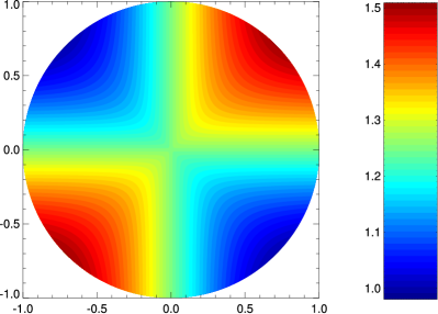
Figure 1.: Visualization of the viscosity structure according to Equation (1), at $t=0$ and with $\nu_{0}=1$, $A=0.25$. nu

Now assume an $m=2$ oscillation of the viscosity [$\nu$], which is to mimic the tidal deformation of the tachocline due to the Venus–Earth–Jupiter cycle (a similar way of emulating tidal driving, by using an $m=2$ body force, was described by Cebron and Hollerbach (2014)). The space-time dependence is assumed to be

$$\nu(r,\phi,t) = \nu_{0}\{1+A[1+0.5r^{2}/R^{2}\sin(2\phi)(1+\cos(2\pi t/T_{\nu}))]\}\;,$$ (1)

which includes a constant term $\nu_{0}(1+A)$ and an additional term with an $m=2$ azimuthal dependence that is oscillating with a period $T_{\nu}$. The spatial structure of $\nu$ is illustrated in Figure nu.

Figure 2.: Three examples of the temporal evolution of the energy, the helicity, and the $\alpha$-effect for $T_{\nu}/T_{0}=0.7,1.06,1.42$. The time is normalized to the viscous time scale, i.e. $t_{n}\equiv t\nu/R^{2}$. zeit

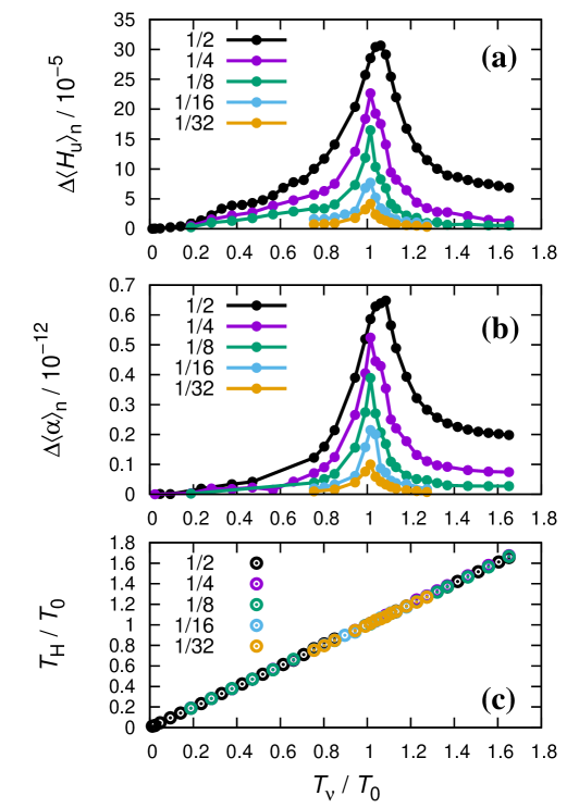
Figure 3.: Resonant excitation of the kinetic helicity and the $\alpha$-effect, connected with the $m=1$ TI, by the $m=2$ viscosity oscillation with five different amplitudes $A=0.03125,0.0625,0.125,0.25,0.5$. Amplitude of the oscillations of helicity (a) and the $\alpha$-effect (b) in dependence on the period of excitation. (c) Oscillation period of helicity in dependence on the period of excitation. parametric

For the intensity of the viscosity wave we choose now five specific values $A=0.03125,0.0625,0.125,0.25,0.5$. For $A=0.5$, and three different oscillation periods $T_{\nu}/T_{0}=0.7,1.06,$ and 1.42, Figure zeit shows the temporal evolution of three quantities. The first row gives the averaged Reynolds number of the flow arising from the initial state at rest, $Re=R(\langle u^{2}\rangle)^{1/2}/\nu$ where $\langle...\rangle$ denotes an average over the total volume. For all three ratios $T_{\nu}/T_{0}$, we get the same $Re\approx 350$ with very small fluctuations superposed on it. In the second row we show the kinetic helicity, as normalized to the mean-squared velocity over radius, i.e., ${\langle H_{u}\rangle}_{n}=\langle{{\mathbfit u}}\cdot(\nabla\times{{\mathbfit u}})\rangle R/\langle u^{2}\rangle$. Apart from some constant part, we observe a significant fluctuation (with exactly the period of the viscosity oscillation), which appears strongest for $T_{\nu}/T_{0}=1.06$. Intimately connected with this helicity oscillation, we also show (third row) the $\alpha$-effect, normalized in such a way that it corresponds to a magnetic Reynolds number of the helical flow part, i.e., ${\langle\alpha\rangle}_{n}=\mu_{0}\sigma R\langle({{\mathbfit u}}\times{{\mathbfit b}})\cdot{{\mathbfit B}}_{0}\rangle/B^{2}_{0}$.

Figure parametric shows the amplitude of the helicity oscillation (a), the corresponding amplitude of the $\alpha$ oscillation (b), and their period (c) as a function of the period of excitation. Evidently we obtain a strong resonance (a,b) when the excitation frequency $1/T_{\nu}$ is equal to the intrinsic “eigenfrequency” $1/T_{0}$ of the helicity oscillation.

Figure tom reveals the character of the helicity oscillations in terms of the velocity for the particular case $T_{\nu}/T_{0}=1.06$. While Figure toma illustrates the averaged velocity field, Figures tomb – d show the residual velocities at maximum, mean, and minimum helicity.

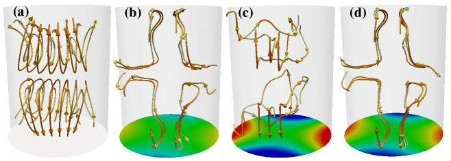
Figure 4.: Velocity field over one half-period of the helicity oscillation for the case $A=0.5$, $T_{\nu}/T_{0}=1.06$. (a) Typical $m=1$ velocity field of the TI, as averaged over one period of the helicity oscillation. (b) Residual velocity (i.e., actual velocity minus averaged velocity), for an instant with maximum helicity. (c) Residual velocity for an instant with mean helicity. (d) Residual velocity for an instant with minimum helicity. The typical velocities of (a) are a factor of 44 larger than those of (b,c,d). Note the opposite directions of the residual velocity in (b) and (d). The color at the bottom of (b,c,d) indicates the viscosity at the respective instants, according to Equation (1). tom

3 Synchronizing the Solar Dynamo

In the previous section, we have seen that a weak $m=2$ viscosity oscillation is able to excite, and synchronize, an oscillation of the helicity and the corresponding $\alpha$-effect with the same frequency.

In this section, a first attempt will be made to set up a closed dynamo model in which the synchronized $\alpha$-effect is appropriately embedded. To keep the physics simple, we will use an extremely reduced, zero-dimensional $\alpha$–$\Omega$ dynamo model consisting of two coupled ordinary differential equations for the toroidal and the poloidal field component. Despite their simplicity, models of this sort have been shown to be well capable of producing various solar-like features (Hoyng, 1993; Weiss and Tobias, 2016), in particular if the induction effects in spatially segregated layers are mimicked by appropriate time delays in the model (Wilmot-Smith et al., 2006).

Specifically, we consider the following system of equations:

$$\frac{{\rm d}a(t)}{{\rm d}t} = \alpha(t)b(t)-a(t)$$ (2)

$$\frac{{\rm d}b(t)}{{\rm d}t} = \Omega a(t)-b(t)$$ (3)

wherein $a$ represents the poloidal field (actually, its vector potential), and $b$ the toroidal magnetic field. While keeping constant the value of $\Omega$, which represents the induction effect of the differential rotation, $\alpha$ is considered as dependent on the instantaneous toroidal magnetic field:

$$\alpha(t) = \frac{c}{1+gb^{2}(t)}+\frac{pb^{2}(t)}{1+hb^{4}(t)}\sin{(2\pi t/T_{\nu})}\;.$$ (4)

Equation (alpha) is motivated as follows: the first term, scaled by $c$, reflects some constant part that is only quenched, in the usual way, by the magnetic-field energy [$b^{2}$] in the denominator. Although this term can be chosen to be quite small, we will see that it must not be set to zero. The second term, scaled by a parameter $p$, is periodic in time and emulates the resonance of the $\alpha$-oscillation in the sense that its explicit temporal dependence is fixed, but its amplitude has a maximum at some particular value of $b$ where the external excitation is in resonance with the intrinsic helicity oscillation of the TI (note that the frequency of the helicity oscillation is a monotonically increasing function of the azimuthal magnetic field; see Figure 7 of Weber et al. (2015)). Interestingly, a similar $b$-dependence of $\alpha$ had already been used by Wilmot-Smith et al. (2006), although without the $\sin{(2\pi t/T_{\nu})}$ dependence, and for other reasons than here.

Figure auto illustrates the evolution of this equation system for six different parameter sets which cover some paradigmatic types of solutions, although not exhaustively. Figures autoa – c correspond to solutions that clearly do not comply with the solar dynamo, while autod – f are much more interesting. In all cases we choose $g=1$ and $T_{\nu}=11.07$ years.

Let us start with Figure autoa, obtained for $\Omega=10$, $c=0$, $p=8$, and $h=10$. Evidently, this dynamo fails to work at all, since the constant part of $\alpha$ is set exactly to zero. The dynamo fails also when some constant $\alpha$ is used (by setting $c=0.8$), but $\Omega=-10$ acquires the wrong sign; see Figure autob. A first dynamo becomes visible in autoc, with $\Omega=10$, $c=0.8$, $p=8$, and a comparably large value $h=20$. However, the fields generated by this dynamo vacillate with a period of 11.07 years around some finite positive values, instead of oscillating with the correct 22.14-year period around zero.

Much more promising results are obtained for $c=0.8$, $p=8$, $h=10$. For increasing values $\Omega=10,50,100$, Figures autod – f show a quite robust solar-type behavior, with an ever increasing ratio $b/a$ (note the different scaling factors for $b$ in the three pictures). The most important point here is that the 11.07 years (Schwabe) periodicity of $\alpha$ leads to the 22.14 years (Hale) oscillation of both $a$ and $b$, in contrast to the mere vacillation seen in Figure autoc.

For the restricted period $27<t<36$ years of Figure autod, the next Figure detail illustrates in more detail the behavior during a sign change of the magnetic field, including the amazing “spiky” features of $\alpha$ close to the turning point of $a$ and $b$. The capitals A…E mark various instants with specific features to be explained in the following: Initially (A), at large values of $b$, $\alpha$ is rather constant, although strongly quenched, while its oscillatory part is negligible since $b$ is so strong that we are far away from resonance. As $b$ decreases, it reaches a level at which the TI helicity oscillation becomes resonant with the viscosity oscillation. This happens (B) when $b\approx 0.56$, which actually corresponds to the maximum of the pre-factor $b^{2}/(1+10b^{4})$ of the oscillatory term in Equation (4). At this point $\alpha$ becomes strongly negative. Shortly after (C), $b$ drops to zero, so that the quenching of the constant term of $\alpha$ disappears and $\alpha$ acquires the unquenched value $c$ (here $\approx 0.8$). Subsequently (D), $b$ goes again through the resonant point $b\approx-0.56$ for the helicity oscillation so that the oscillatory part again contributes its large, but now positive, value to $\alpha$. After that (E), $b$ increases quite smoothly until it reaches a maximum strength where $\alpha$ is strongly quenched and rather constant.

It is worth noting that many oscillatory dynamo solutions, based on Equations (2,3) and some appropriate quenching of $\alpha$, show a similar behavior as long as the quenching of $\alpha$ is quadratic in the fields. This applies, e.g., to some of the solutions given by Wilmot-Smith et al. (2006) where a close connection with a driven oscillator, in which the driving works only in a certain window of $b$, has been discussed. In some sense, the resonant driving of $\alpha$ with the 11-year cycle can thus be considered just a trigger for the whole process.

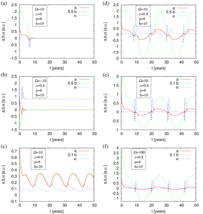
Figure 5.: Evolution of the equation system (2) – (4) with $g=1$ and $T_{\nu}=11.07$ years. All other parameters are given in the insets. auto

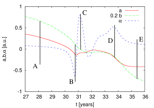
Figure 6.: Details of Figure autod (but note the different scaling of $b$). For explanations of situations A…E, see the text. detail

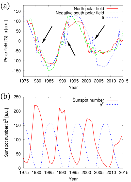
Figure 7.: (a) Comparison of the north and south polar magnetic field and the parameter $a$, appropriately scaled and shifted in time. The field data are the 20 nHz filtered data from Wilcox Solar Observatory (courtesy J.T. Hoeksema). (b) Comparison of the mean sunspot number and the parameter $b^{2}$, appropriately scaled and shifted in time. The sunspot data are SILSO data from the Royal Observatory of Belgium, Brussels. solar

In Figure solar we compare our simulations with two specific time series of the observed solar magnetic field. For this purpose we restrict the time to the period between 1975 and 2015 for which north and south polar-field data are available from the Wilcox Solar Observatory. Figure solara shows the 20 nHz filtered north and south polar-field data, together with an appropriately scaled and time-shifted segment of our $a(t)$. For the same period, Figure solarb shows the annual sunspot number, obtained from the Royal Observatory of Belgium, Brussels, together with our $b^{2}(t)$.

The first observation that we make in Figures auto, detail, and solar is the in-phase behavior of $a$ and $b$ which looks not very solar-like at first glance. In reality (see Figures solara and b), the solar magnetic field shows a significant phase-shift between the sunspot activity (a tracer for the toroidal field), and the global poloidal dipole field.

A possible way out of this dilemma is to invoke the rise-time of the toroidal field, in terms of flux tubes, from the tachocline to the photosphere. Figure solarb would point to a rise-time of approximately four years. According to Figure 2 of Weber, Fan, and Miesch (2013), this would be roughly consistent with a magnetic-field strength of 15 kG for a tube simulation without convection. Unfortunately, the inclusion of convection leads to rise times not longer than eight months. Here lies one of the crucial point for the acceptability of this sort of dynamo localized in, or at least close to the tachocline, while flux-transport dynamos, or dynamos in which this spatial separation is emulated by a time-delay (Wilmot-Smith et al., 2006) can easily comply with this long time-shift. Only later simulations will show if this discrepancy can be overcome in higher dimensional $\alpha$–$\Omega$ models.

An amazing coincidence exists, however, between the additional peaks of the north and south polar field in Figure solara and the corresponding spikes of our $a$ (indicated by the three black arrows).

Another point is related to the vigorous, ”spiky” variations of $\alpha$ close to the reversal point of $a$ and $b$, as seen in Figure auto and Figure detail. It is tempting to relate this behavior to the short-term sign changes of the current-helicity, as observed recently by Zhang et al. (2012). It might also be interesting to relate the high amplitudes of $\alpha$ to the so-called $\delta$-sunspots, while other explanations in terms of kink-type instabilities of flux-tubes have also been invoked to explain them (Fan, 2009).

While it is not our intention to overemphasize the significance of the latter two points, they might be kept in mind when trying to validate, or falsify, our resonant synchronization model of the solar cycle.

4 Conclusions and Outlook

While the traditional explanation of the Hale cycle bears on intrinsic and, in general, time-independent features of the solar dynamo such as the magnetic diffusivity, the amplitudes of $\Omega$, $\alpha$, and the meridional flow (Charbonneau and Dikpati, 2000), we have asked for a mechanism that could allow for synchronizing the solar dynamo with planetary tides. From the very outset we were well aware of the fact that those tiny forces could never compete with the much larger acceleration forces of the turbulent motion in the convection zone (if this were indeed the governing source of the $\alpha$-effect). The same holds true for a corresponding $\alpha$-effect based on a Babcock–Leighton mechanism. However, an additional energy injection from an external forcing is not the crucial point in our argumentation.

Motivated by the recent numerical evidence of helicity oscillations appearing in the kink-type, $m=1$ TI (Weber et al., 2015), we studied a simple cylindrical model for the resonant excitation of those oscillations by an $m=2$ viscosity variation that serves as a proxy for the tidal action of planetary forces. Invoking, as a specific example, the 11.07-year periodic tide produced by the Venus–Earth–Jupiter system, this was shown to trigger a 11.07-year oscillation of the helicity and the related $\alpha$-effect. This resonant excitation of the $\alpha$-oscillation served then as a “clock” for the 22.14-year dynamo cycle of a reduced, zero-dimensional $\alpha-\Omega$ dynamo model. The output of this model shows interesting solar-like features, in particular an additional secondary peak of the poloidal field shortly after its sign change, and a tendency for vigorous and fast oscillations of the helicity in this weak-field period.

As already mentioned by Weber et al. (2015), there is nearly no external energy needed to trigger helicity oscillations. As an intrinsic feature of the TI, a helicity oscillation is just a reshuffling of (kinetic and magnetic) energy between left- and right-handed modes, without (or barely) changing the energy content, as confirmed in Figure zeit. Exactly here is the point where the tiny planetary forces might get a chance to synchronize the solar dynamo. Since this type of dynamo draws its energy nearly exclusively from the shear of the differential rotation, the resonantly oscillating $\alpha$-effect functions as a periodically opening “bottleneck” that ultimately controls the frequency of the dynamo. An interesting and non-trivial next step would be to check if also longer periods of the solar dynamo, like the $\approx 87$-year Gleissberg cycle, the $\approx 210$-year Suess-de-Vries cycle, and the $\approx 2300$-year Hallstatt cycle, can be explained somehow in the framework of the present model.

It goes without saying that the delineated mechanism is by far not the end of the story. What is urgently needed is to blend together the two mechanisms, which were only loosely connected in this article, into an appropriate global, i.e. at least a 1D, or better a 2D, or 3D dynamo model. Perhaps the most significant problem of our model is the complete omission of rotation and gravity. The TI has been treated only in the presence of viscosity and resistivity, so that the typical growth rates and frequencies are $\propto\omega^{2}_{\rm{Alfven}}/\omega_{\eta}$ (Rüdiger, Kitchatinov, and Hollerbach, 2013). This will definitely be modified when rotation and stratification are taken into account. Hopefully, the main result will not change very dramatically. As shown recently (Rüdiger et al., 2015; Stefani and Kirillov, 2015), the effect of positive shear in the tachocline (which prevails in a $\pm 30^{\circ}$ strip around the Equator) on the TI is not so grave and leads, surprisingly, even to some moderate reduction of the critical Hartmann number. The azimuthal drift of the instability mode depends strongly on the radial profile of $B_{\phi}(r)$, tending to corotate for $B_{\phi}(r)\propto 1/r$ while standing still for $B_{\phi}(r)\propto r$ (Rüdiger et al., 2015).

A final remark: Leaving aside the specific TI aspect of the helicity oscillations and their resonant excitation, as discussed in Section 2, one might ask for other realizations of the general resonance model as described in Section 3. Specifically, it is worthwhile to check whether a similar resonance could apply to a tachocline $\alpha$, as proposed by Dikpati and Gilman (2001). In any case, the model according to Equations (2) – (4) would then change significantly due to the missing dependence of the eigenfrequency on the magnetic-field strength, which is indeed a specific feature of the TI based synchronization model as presented here.

Acknowledgments

This work was supported by the Deutsche Forschungsgemeinschaft in the frame of the SPP 1488 (PlanetMag), as well as by Helmholtz-Gemeinschaft Deutscher Forschungszentren (HGF) in frame of the Helmholtz alliance LIMTECH. Wilcox Solar Observatory data used in this study was obtained via the web site wso.stanford.edu (courtesy of J.T. Hoeksema). The sunspot data are SILSO data from the Royal Observatory of Belgium, Brussels, obtained via www.sidc.be/silso/infosnytot. F. Stefani thanks R. Arlt, A. Bonnano, A. Brandenburg, A. Choudhuri, D. Hughes, M. Gellert, G. Rüdiger, and D. Sokoloff for fruitful discussion on the solar-dynamo mechanism.

Disclosure of Potential Conflicts of Interest

The authors declare that they have no conflicts of interest.

Appendix A The Numerical Model

In this appendix we sketch the integro-differential equation scheme that was utilized in Section 2 for the calculation of the oscillations of the helicity and $\alpha$. Further details can be found in Weber et al. (2013, 2015). For an alternative numerical method to treat the TI, see Herreman et al. (2015).

In our code we circumvent the usual $Pm$ limitations of pure differential-equation codes by replacing the solution of the induction equation for the magnetic field by invoking the so-called quasistatic approximation (Davidson, 2001). We replace the explicit time stepping of the magnetic field by computing the electrostatic potential by a Poisson solver, and deriving the electric-current density. In contrast to many other inductionless approximations in which this procedure is sufficient, in our case we cannot avoid to compute the induced magnetic field, too. The reason for this is the presence of an externally applied electrical current in the fluid. Computing the Lorentz-force term it turns out that the product of the applied current with the induced field is of the same order as the product of the magnetic field (due to the applied current) with the induced current. The induced magnetic field is computed as follows: in the interior of the domain, we apply the quasi-stationary approximation and solve the vectorial Poisson equation for the magnetic field which results when the temporal derivative in the induction equation is set to zero. At the boundary of the domain, however, the induced magnetic field is computed from the induced current density by means of Biot–Savart’s law. This way we arrive at an integro-differential equation approach, similar to the method used by Meir et al. (2004).

In detail, the numerical model as developed by Weber et al. (2013) works as follows: it uses the OpenFOAM library to solve the Navier–Stokes equations (NSE) for incompressible fluids

eqn:navierstokes$$\dot{{\mathbfit u}}+\left({{\mathbfit u}}\cdot\nabla\right){{\mathbfit u}}=-\nabla p+\nu\Delta{{\mathbfit u}}+\frac{{\mathbfit f}_{\mathrm{L}}}{\rho}\hskip 14.22636pt\textrm{and}\hskip 14.22636pt\nabla\cdot{\mathbfit u}=0,$$ (5)

with ${\mathbfit u}$ denoting the velocity, $p$ the (modified) pressure, ${\mathbfit f}_{\mathrm{L}}={\mathbfit J}\times{\mathbfit B}$ the electromagnetic Lorentz force density, ${\mathbfit J}$ the total current density, and ${\mathbfit B}$ the total magnetic field. The NSE is solved using the PISO algorithm and applying no slip boundary conditions at the walls.

Ohm’s law in moving conductors

$${{\mathbfit j}}=\sigma\left(-\nabla\varphi+{{\mathbfit u}}\times{{\mathbfit B}}\right)$$ (6)

allows us to compute the induced current ${\mathbfit j}$ by previously solving a Poisson equation for the perturbed electric potential $\varphi=\phi-J_{0}z/\sigma$:

$$\Delta\varphi=\nabla\cdot\left({{\mathbfit u}}\times{{\mathbfit B}}\right).$$ (7)

We concentrate now on cylindrical geometries with an axially applied current. After subtracting the (constant) potential part [$J_{0}z/\sigma$], with $z$ as the coordinate along the cylinder axis, we use the simple boundary condition $\varphi=0$ on top and bottom and ${\mathbfit n}\cdot\nabla\varphi=0$ on the mantle of the cylinder, with $\bf n$ as the surface normal vector.

The induced magnetic field at the boundary of the domain can then be calculated by Biot–Savart’s law

eqn:biotsavart$${{\mathbfit b}}({{\mathbfit r}})=\frac{\mu_{0}}{4\pi}\int dV^{\prime}\,\frac{{{\mathbfit j}}({{\mathbfit r}}^{\prime})\times({{\mathbfit r}}-{{\mathbfit r}}^{\prime})}{\left|{{\mathbfit r}}-{{\mathbfit r}}^{\prime}\right|^{3}}.$$ (8)

In the bulk of the domain, the magnetic field is computed by solving the vectorial Poisson equation

eqn:induction$$\Delta{{\mathbfit b}}=\mu_{0}\sigma\nabla\times({{\mathbfit u}}\times{{\mathbfit B}})$$ (9)

which results from the full time-dependent induction equation in the quasi-stationary approximation.

Knowing ${\mathbfit b}$ and ${\mathbfit j}$ we compute the Lorentz force ${{\mathbfit f}}_{\mathrm{L}}$ for the next iteration. For more details about the numerical scheme, see Section 2 and 3 of Weber et al. (2013).

References

- Abreu et al. (2012) Abreu, J.A., Beer, J., Ferriz-Mas, A., McCracken, K.G., Steinhilber, F.: 2012, Is there a planetary influence on solar activity? Astron. Astrophys. 548, A88 DOI.
- Babcock (1961) Babcock, H.W.: 1961, The topology of the suns magnetic field and the 22-year cycle. Astrophys. J. 133, 572 DOI.
- Bollinger (1952) Bollinger, C.J.: 1952, A 44.77 year Jupiter-Venus-Earth configuration sun-tide period in solar-climatic cycles. Proc. Okla. Acad. Sci. 33, 307.
- Bonanno et al. (2012) Bonanno, A., Brandenburg, A., Del Sordo, F., Mitra, D.: 2012, Breakdown of chiral symmetry during saturation of the Tayler instability. Phys. Rev. E 86, 016313 DOI.
- Brandenburg (2005) Brandenburg, A.: 2005, The case for a distributed solar dynamo shaped by near-surface shear. Astrophys. J. 625, 625 DOI.
- Brown et al. (1989) Brown, T.M, Christensen-Dalsgaard, J., Dziembowski, W.A., Goode, P., Gough, D.O., Morrow, C.: 1989, Inferring the sun’s internal angular velocity from observed p-mode frequency splitting. Astrophys. J. 343, 526 DOI.
- Callebaut, de Jager, and Duhau (2012) Callebaut, D.K., de Jager, C., Duhau, S.: 2012, The influence of planetary attractions on the solar tachocline. J. Atmos. Sol.-Terr. Phys. 80, 73 DOI.
- Cebron and Hollerbach (2014) Cebron, D., Hollerbach, R.: 2014, Tidally driven dynamos in a rotating sphere. Astrophys. J. Lett. 789, L25 DOI.
- Charbonneau (2010) Charbonneau, P.: 2010, Dynamo models of the solar cycle. Liv. Rev. Solar Phys. 7, 3 DOI.
- Charbonneau and Dikpati (2000) Charbonneau, P., Dikpati, M.: 2000, Stochastic fluctuations in a Babcock-model of the solar cycle. Astrophys. J. 543, 1027 DOI.
- Charvatova (1997) Charvatova, I.: 1997, Solar-terrestrial and climatic phenomena in relation to solar inertial motion. Surv. Geophys. 18, 131 DOI.
- Chatterjee et al. (2011) Chatterjee, P., Mitra, D., Brandenburg, A., Rheinhardt, M.: 2011, Spontaneous chiral symmetry breaking by hydromagnetic buoyancy. Phys. Rev. E 84, 025403 DOI.
- Chiba and Tosa (1990) Chiba, M., Tosa, M.: 1990, Swing excitation of galactic magnetic-fields induced by spiral density waves. Mon. Not. Roy. Astron. Soc. 244, 714 DOI.
- Choudhuri, Schüssler, and Dikpati (1995) Choudhuri, A.R., Schüssler, M., Dikpati, M.: 1995, The solar dynamo with meridional circulation. Astron. Astrophys. 303, L29.
- Choudhuri and Karak (2009) Choudhuri, A.R., Karak, B.B.: 2009, A possible explanation of the Maunder minimum from a flux transport dynamo model. Res. Astron. Astrophys. 9, 953.
- Cole (1973) Cole, T.W.: 1973, Periodicities in solar activities. Solar Phys. 30, 103 DOI.
- Condon and Schmidt (1975) Condon, J.J., Schmidt, R.R.: 1975, Planetary tides and the sunspot cycles. Solar Phys. 42, 529 DOI.
- Courvoisier, Hughes, and Tobias (2012) Courvoisier, A., Hughes, D.W., Tobias, S.M.: 2006, effect in a family of chaotic flows. Phys. Rev. Lett. 96, 034503 DOI.
- Davidson (2001) Davidson, P.A.: 2001, An introduction to magnetohydrodynamics, Cambridge University Press, Cambridge.
- De Jager and Versteegh (2005) De Jager, C., Versteegh, G.: 2005, Do planetary motions drive solar variability? Solar Phys. 229, 175 DOI.
- Dikpati and Gilman (2001) Dikpati, M., Gilman, P.: 2001, Flux-transport dynamos with alpha-effect from global instability of tachocline differential rotation: A solution for magnetic parity selection in the sun. Astrophys. J. 559, 428 DOI.
- D’Silva and Choudhuri (1993) D’Silva, S., Choudhuri, A.R.: 1993, A theoretical model for tilts of bipolar magnetic regions. Astron. Astrophys. 272, 621.
- Fan (2009) Fan, Y.: 2009, Magnetic fields in the solar convection zone. Liv. Rev. Solar Phys. 6, 4 DOI.
- Ferriz Mas, Schmitt, and Schüssler (1994) Ferriz Mas, A., Schmitt, D., Schüssler, M.: 1994, A dynamo effect due to instability of magnetic flux tubes. Astron. Astrophys. 289, 949.
- Gellert, Rüdiger, and Hollerbach (2011) Gellert, M., Rüdiger, G., Hollerbach, R.: 2011, Helicity and alpha-effect by current-driven instabilities of helical magnetic fields. Mon. Not. Roy. Astron. Soc. 414, 2696 DOI.
- Giesecke, Stefani, and Burguete (2012) Giesecke, A., Stefani, F., Burguete, J.: 2012, Impact of time-dependent nonaxisymmetric velocity perturbations on dynamo action of von Kármán-like flows. Phys. Rev. E 86, 066303 DOI.
- Gray et al. (2010) Gray, L.J., Beer, J., Geller, M., Haigh, J.D., Lockwood, M., Matthes, K., Cubasch, U., Fleitmann, D., Harrison, G., Hood, L., Luterbacher, J., Meehl, G.A., Shindell, D., van Geel, B., White, W.: 2010, Solar inluences on climate. Rev. Geophys. 48, RG4001 DOI.
- Herreman et al. (2015) Herreman, W., Nore, C., Cappanera, L., Guermond, J.-L.: 2015, Tayler instability in liquid metal columns and liquid metal batteries. J. Fluid Mech. 771, 79 DOI.
- Hoyng (1993) Hoyng, P.: 1993, Helicity fluctuations in mean-field theory: an explanation for the variability of the solar cycle?. Astron. Astrophys. 272, 321.
- Hung (2007) Hung, C.-C.: 2007, Apparent relations between solar activity and solar tides caused by the planets. NASA/TM. 2007-214817, 1.
- Jiang, Chatterjee, and Choudhuri (2007) Jiang, J., Chatterjee, P., Choudhuri, A.R.: 2007, Solar activity forecast with a dynamo model. Mon. Roy. Astron. Soc. 381, 1527 DOI.
- Jose (1965) Jose, P.D.: 1965, Suns motion and sunspots. Astron. J. 70, 193 DOI.
- Krause and Rädler (1980) Krause, F., Rädler, K.-H.: 1980, Mean-field magnetohydrodynamics and dynamo theory, Akademie-Verlag, Berlin.
- Leighton (1964) Leighton, R.B.: 1964, Transport of magnetic field on the sun. Astrophys. J. 140, 1547 DOI.
- Meir et al. (2004) Meir, A.J., Schmidt, P.G., Bakhtiyarov, S.I., Overfelt, R.A.: 2004, Numerical simulation of steady liquid – metal flow in the presence of a static magnetic field. J. Appl. Mech. 71, 786 DOI.
- Okhlopkov (2014) Okhlopkov, V.P.: 2014, The 11-year cycle of solar activity and configurations of the planets. Mosc. U. Phys. B. 69, 257 DOI.
- Palus et al. (2000) Palus, M., Kurths, J., Schwarz, U., Novotna, D., Charvatova, I.: 2000, Is the solar activity cycle synchronized with the solar inertial motion? Int. J. Bifurc. Chaos 10, 2519 DOI.
- Parker (1955) Parker, E.N.: 1955, Hydromagnetic dynamo models. Astrophys. J. 122, 293 DOI.
- Pikovsky, Rosenblum, and Kurths (2001) Pikovsky, A., Rosenblum, M., Kurths, J.: 2001, Synchronizations: A universal concept in nonlinear sciences, Cambridge University Press, Cambridge.
- Pitts and Tayler (1985) Pitts, E., Tayler, R.J.: 1985, The adiabatic stability of stars containing magnetic-fields. 6. The influence of rotation. Mon. Not. Roy. Astron. Soc. 216, 139 DOI.
- Proctor (2006) Proctor, M.: 2006, Dynamo action and the sun. EAS Publications Series 21, 241 DOI.
- Rädler and Stepanov (2006) Rädler, K., Stepanov, R.: 2006, Mean electromotive force due to turbulence of a conducting fluid in the presence of mean flow. Phys. Rev. E 73, 056311 DOI.
- Rüdiger, Kitchatinov, and Hollerbach (2013) Rüdiger, G., Kitchatinov, L.L., Hollerbach, R.: 2013, Magnetic processes in astrophysics, Wiley-VCH, Berlin.
- Rüdiger et al. (2015) Rüdiger, G., Schultz, M., Gellert, M., Stefani, F.: 2015, Subcritical excitation of the current-driven Tayler instability by super-rotation. Phys. Fluids 28, 014105 DOI.
- Scafetta (2010) Scafetta, N.: 2010, Empirical evidence for a celestial origin of the climate oscillations and its implications. J. Atmos. Sol.-Terr. Phys. 72, 951 DOI.
- Scafetta (2014) Scafetta, N.: 2014, The complex planetary synchronization structure of the solar system. Pattern Recogn. Phys. 2, 1 DOI.
- Schmitt, Schüssler, and Ferriz Mas (1996) Schmitt, D., Schüssler, M., Ferriz Mas, A.: 1996, Intermittent solar activity by an on-off dynamo. Astron. Astrophys. 311, L1.
- Seilmayer et al. (2012) Seilmayer, M., Stefani, F., Gundrum, T., Weier, T., Gerbeth, G., Gellert, M., Rüdiger, G.: 2012, Experimental evidence for Tayler instability in a liquid metal column. Phys. Rev. Lett. 108, 244501 DOI.
- Spruit (2002) Spruit, H.: 2002, Dynamo action by differential rotation in a stably stratified stellar interior. Astron. Astrophys. 381, 923 DOI.
- Steenbeck and Krause (1969) Steenbeck, M., Krause, F.: 1969, Zur Dynamotheorie stellarer und planetarer Magnetfelder. I. Berechnung sonnenähnlicher Wechselfeldgeneratoren. Astron. Nachr. 291, 49 DOI.
- Steenbeck, Krause, and Rädler (1966) Steenbeck, M., Krause, F., Rädler, K.-H.: 1966, Berechnung der mittleren Lorentz-Feldstärke vxB für ein elektrisch leitendes Medium in turbulenter durch Coriolis-Kräfte beeinflusster Bewegung. Z. Naturforsch. A 21(4), 369 DOI.
- Stefani and Kirillov (2015) Stefani, F., Kirillov, O.N.: 2015, Destabilization of rotating flows with positive shear by azimuthal magnetic fields. Phys. Rev. E 92, 051001(R) DOI.
- Stix (1972) Stix, M.: 1972, Nonlinear dynamo waves. Astron. Astrophys. 20, 9.
- Svensmark and Friis-Christensen (1997) Svensmark, H., Friis-Christensen, E.: 1997, Variation of cosmic ray flux and global cloud coverage - a missing link in solar-climate relationships. J. Atmos. Sol.-Terr. Phys. 59, 1225 DOI.
- Takahashi (1968) Takahashi, K.: 1968, On the relation between the solar activity cycle and the solar tidal force induced by the planets. Solar Phys. 3, 598 DOI.
- Tayler (1973) Tayler, R.J.: 1973, The adiabatic stability of stars containing magnetic fields-I: Toroidal fields. Mon. Not. Roy. Astron. Soc. 161, 365 DOI.
- Vainshtein and Cattaneo (1992) Vainshtein, S.I., Cattaneo, F.: 1992, Nonlinear restrictions on dynamo action. Astrophys. J. 393, 165 DOI.
- Weber, Fan, and Miesch (2013) Weber, M.A., Fan, Y., Miesch, M.S.: 2013, Comparing simulations of rising flux tubes through the solar convection zone with observations of solar active regions: Constraining the dynamo field strength. Solar Phys. 287, 239 DOI.
- Weber et al. (2013) Weber, N., Galindo, V., Stefani, F., Weier, T., Wondrak, T.: 2013, Numerical simulation of the Tayler instability in liquid metals. New J. Phys. 15, 043034 DOI.
- Weber et al. (2015) Weber, N., Galindo, V., Stefani, F., Weier, T.: 2015, The Tayler instability at low magnetic Prandtl numbers: between chiral symmetry breaking and helicity oscillations. New J. Phys. 17, 113013 DOI.
- Weiss and Tobias (2016) Weiss, N.O., Tobias, S.M: 2016, Supermodulation of the Sun’s magnetic activity: the effect of symmetry changes. Mon. Not. Roy. Astron. Soc. 456, 2654 DOI.
- Wilmot-Smith et al. (2006) Wilmot-Smith, A.L., Nandy, D., Hornig, G., Martens, P.C.H.: 2006, A time delay model for solar and stellar dynamos. Astrophys. J. 652, 696 DOI.
- Wilson (2013) Wilson, I.R.G.: 2013, The Venus-Earth-Jupiter spin-orbit coupling model. Pattern Recogn. Phys. 1, 147 DOI.
- Wood (1972) Wood, K.: 1972, Sunspots and planets. Nature 240(5376), 91 DOI.
- Yoshimura (1975) Yoshimura, H.: 1975, Solar-cycle dynamo wave propagation. Astrophys. J. 201, 740 DOI.
- Zahn, Brun, and Mathis (2007) Zahn, J.-P., Brun, A.S., Mathis, S.: 2007, On magnetic instabilities and dynamo action in stellar radiation zones. Astron. Astrophys. 474, 145 DOI.
- Zhang et al. (2012) Zhang, H., Moss, D., Kleeorin, N., Kuzanyan, K., Rogachevskii, I., Sokoloff, D., Gao, Y., Xu, H.: 2012, Current helicity of active regions as a tracer of large-scale solar magnetic helicity. Astrophys. J. 751 DOI.
- Zhang et al. (2003) Zhang, K., Chan, K.H., Zou, J., Liao, X., Schubert, G.: 2003, A three-dimensional spherical nonlinear interface dynamo. Astrophys. J. 596, 663 DOI.