Ducks in space: from nonlinear absolute instability to noise-sustained structures in a pattern-forming system

Abstract

A subcritical pattern-forming system with nonlinear advection in a bounded domain is recast as a slow-fast system in space and studied using a combination of geometric singular perturbation theory and numerical continuation. Two types of solutions describing the possible location of stationary fronts are identified, whose origin is traced to the onset of convective and absolute instability when the system is unbounded. The former are present only for nonzero upstream boundary conditions and provide a quantitative understanding of noise-sustained structures in systems of this type. The latter correspond to the onset of a global mode and are present even with zero upstream boundary condition. The role of canard trajectories in the nonlinear transition between these states is clarified and the stability properties of the resulting spatial structures are determined. Front location in the convective regime is highly sensitive to the upstream boundary condition and its dependence on this boundary condition is studied using a combination of numerical continuation and Monte Carlo simulations of the partial differential equation. Statistical properties of the system subjected to random or stochastic boundary conditions at the inlet are interpreted using the deterministic slow-fast spatial-dynamical system.

1 Introduction

Systems of hydrodynamic type with through-flow are well-known to be highly sensitive to the upstream boundary condition. In some systems this is a consequence of the non-normality of the linear stability operator; such operators can greatly amplify small perturbations even when the base flow is linearly stable, resulting in transient amplification [34]. In others it is a consequence of convective instability within the linear stability problem, i.e., an instability that grows in an appropriately moving reference frame, although it decays at any fixed downstream location. As a result, continued injection of fluctuations at the upstream boundary leads to the presence of a noise-sustained structure downstream [11]. When the source of fluctuations is shut off these structures are swept out of the system, i.e., the downstream disturbance at any fixed location decays to zero. In many systems both processes may be active simultaneously.

When perturbations grow at fixed location we speak instead of absolute instability. Evidently, convective instability must precede absolute instability since the latter requires a sufficiently large growth rate that an initially localized disturbance can expand upstream against downstream advection. Structures associated with absolute instability are no longer sensitive to the upstream boundary condition.

The present paper seeks to investigate the consequences of convective instability in nonlinear systems. Of particular interest are systems exhibiting subcritical absolute instability, a situation that arises frequently in shear flow problems [40]. In such systems the base state may be convectively unstable but finite amplitude perturbations can result in nonlinear absolute instability, i.e., nonlinear states that are no longer swept downstream. We are particularly interested in elucidating the transition from convective to absolute instability in the nonlinear regime, and the associated changes in the sensitivity of the observed structures to the upstream boundary condition.

Nonlinear noise-sustained structures have been studied by direct numerical simulations while most of the large body of work associated with shear flows focuses on structures generated by nonlinear absolute instability. However, the transition between the two has not, to our knowledge, been the subject of any past study. Owing to the difficulty of the subject we choose to investigate here a particular system that is known to display the required properties. For this purpose we select a model first studied by Chomaz & Couairon [9, 10]:

(1.1) $$A_{t}=A_{xx}-(U-\alpha A^{2})A_{x}+\mu A-A^{3}.$$

In this partial differential equation (PDE) $A$ is a real variable representing the amplitude of a nonlinear state and $U$, $\alpha$ and $\mu$ are control parameters. The parameter $U$ measures the strength of advection while $\mu$ is considered to be the principal bifurcation parameter: on the real line the onset of convective instability of the trivial state $A=0$ occurs at $\mu=0$ while the onset of absolute instability takes place at $\mu=\mu_{\rm a}:=U^{2}/4$. Finally, the coefficient $\alpha$ quantifies the importance of the nonlinear correction to the advection velocity $U$. Although this model cannot be derived from the Navier-Stokes equation by standard multiple scale techniques (except near degeneracies) it is faithful to the physics of this class of problems as well as being simple enough to be amenable to relatively complete analysis, and in particular to phase plane techniques.

Chomaz & Couairon posed the above problem on a finite domain, $x\in[0,L]$, subject to Dirichlet boundary conditions $A(0,t)=A(L,t)=0$, and studied the strong advection regime $U\gg 1$. The trivial homogeneous steady state is unstable for sufficiently large values of the control parameter $\mu$, and a subcritical bifurcation at $\mu=\mu_{\rm g}>\mu_{\rm a}$ gives rise to a branch of stationary states with sharp spatial gradients and an $\mathcal{O}(\mathchoice{{\hbox{$\displaystyle\sqrt{\mu\,}$}\lower 0.4pt\hbox{\vrule height=4.30554pt,depth=-3.44446pt}}}{{\hbox{$\textstyle\sqrt{\mu\,}$}\lower 0.4pt\hbox{\vrule height=4.30554pt,depth=-3.44446pt}}}{{\hbox{$\scriptstyle\sqrt{\mu\,}$}\lower 0.4pt\hbox{\vrule height=3.01389pt,depth=-2.41113pt}}}{{\hbox{$\scriptscriptstyle\sqrt{\mu\,}$}\lower 0.4pt\hbox{\vrule height=2.15277pt,depth=-1.72223pt}}})$ amplitude (see Figure 1(a), which is adapted from a sketch by Chomaz & Couairon [10]). We study this model in the case where the inlet boundary condition is small, but nonzero, $0<|A(0,t)|=\eta\ll 1$, while also focusing on the strong advection regime $U\gg 1$. For numerical illustrations we take $U=12$ (hence $\mu_{\textrm{a}}=36$) and $L=10\pi$, unless otherwise stated. The remaining parameters are assumed to be of order one. The main results of our paper can be summarized as follows:

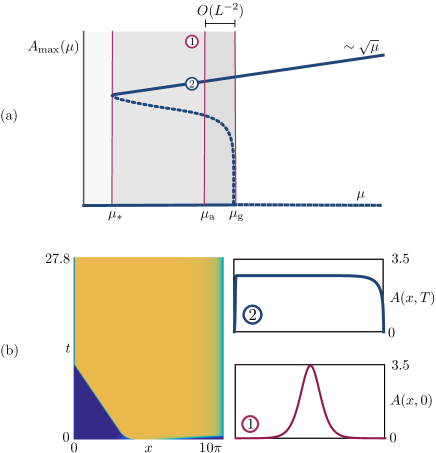
Figure 1: (a) Sketch of the bifurcation diagram of steady states of Eq. (1.1) with Dirichlet boundary conditions $A(0,t)=A(L,t)\equiv 0$, adapted from [10]. (b) Time simulation of (1.1) with Dirichlet boundary conditions. Left: space-time plot for $(x,t)\in[0,L]\times[0,T]$ with $L=10\pi$ and $T=0.21$. Right: initial (1) and final (2) profiles of the time simulation. These states are also marked on the bifurcation diagram in (a). Parameters: $\mu=7.4<\mu_{\mathrm{a}}$, $\alpha=5$, $U=12$.

1. The model (1.1) displays high sensitivity to $\eta$, as documented in Figure 2, where the formation of a front between the base state and the finite amplitude state is shown in a sequence of space-time plots for different values of $\eta$.

2. Numerical continuation of steady states for $\eta\neq 0$ reveals the presence of two types of finite amplitude states, one originating in the convective instability threshold $\mu=0$ and the other in the absolute instability threshold at $\mu=\mu_{\rm g}$. The former reveal extreme sensitivity to the value of $\eta$ and disappear abruptly as $\eta\rightarrow 0^{+}$ (Figure 3).

3. The observed sensitivity to the parameter $\eta$ finds a natural explanation in the presence of canard segments (see below for a definition) on solutions of the spatial boundary value problem (BVP) for the steady states of (1.1). These results are obtained by recasting the BVP as a slow-fast system in space subject to the boundary conditions $A(0,t)=\eta$, $A(L,t)=0$. The solutions of this BVP correspond to finite length trajectories of a slow-fast spatial-dynamical system of van der Pol type.

4. The stability in time of all steady solutions of the BVP is determined and corroborated using direct numerical simulations.

5. Numerical evidence is presented that demonstrates that the statistics of the front location in the convectively unstable regime can be explained solely in terms of the properties of the new branches of steady states in the convectively unstable regime, present for $\eta\neq 0$.

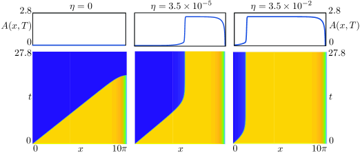
Figure 2: Small variations of the inlet boundary condition $A(0,t)=\eta$ have a dramatic impact on the steady states attained in Eq. (1.1). Left: when we time-step (1.1) starting from a solution with zero inlet boundary condition, $\eta=0$, the system evolves towards the trivial steady state. Center: with $\eta=3.5\times 10^{-5}$ a new solution is selected. Right: a similar final steady state, with a longer plateau, is attained with $\eta=3.5\times 10^{-2}$. Parameters: $\mu=6$, $\alpha=5$, $U=12$, with $(x,t)\in[0,10\pi]\times[0,2.5]$. In all cases $A(L,t)=0$.

As emphasized above, the slow-fast structure of the van der Pol spatial-dynamical system plays an important role in understanding the dynamics of the system. In recent years there has been a great deal of interest in slow-fast systems [18]. Among the many phenomena such systems exhibit is the canard phenomenon [2, 26]. This term is used to refer to the abrupt growth of a limit cycle that occurs, in planar systems, in exponentially narrow parameter intervals. Within this interval the limit cycle follows for a time a repelling slow manifold [20]. Such cycles are known to occur in the van der Pol system, and have been studied intensively in the past [2, 26]. In the following we use the term canard segment to refer to the part of a solution that follows a repelling slow manifold; depending on the situation, such a segment can be part of a periodic solution or not. A maximal canard segment follows a repelling slow manifold for as long as it exists; for example, in the van der Pol oscillator, a maximal canard segment (which is part of a limit cycle) follows the middle (repelling) branch of the cubic nullcline from the lower fold point all the way to the upper one. Phenomena of this type are invariably studied in the time domain, however, and in this paper we seek to extend the slow-fast decomposition to solutions that evolve in space, forming, for example, a front separating two distinct states of the system. However, in the spatial-dynamics formulation one is typically not interested in a periodic state: such systems are typically BVPs with non-periodic boundary conditions. For example, orbits corresponding to steady states of (1.1) may be required to satisfy $A(0)=\eta\neq 0=A(L)$ and the familiar van der Pol canard cycles are not observable in this setting. We eschew here the rigorous construction of such orbits and instead employ phase plane analysis combined with numerical bifurcation analysis to construct relevant orbits of the slow-fast system and to provide numerical evidence for the existence of canard segments.

In addition, we study the stability in time of the steady states of (1.1); in other words, we are interested in canard-like phenomena in the context of PDEs. Amongst the few studies in this direction, we mention canard traveling waves, which have been analyzed in a moving frame as homoclinic connections with a canard segment [5, 23, 37], shock-like structures in PDEs which can also be interpreted in terms of canards [6, 41] and canard-related bifurcation delay in reaction-diffusion PDEs [17, 25]. In recent work we classified for the first time spatio-temporal canards in an infinite-dimensional dynamical system arising in neuroscience applications, using an interfacial dynamics approach [1]. We leave the mathematical study of purely temporal canards in PDEs, such as those reported by Gandhi et al. [21], to future work.

The paper is organized as follows. In Section 2 we provide a brief summary of the results of Chomaz & Couairon. In Section 3 we show how the equation can be cast into a slow-fast system suitable for phase-plane analysis. The phase-plane analysis itself is presented in Section 4 with additional details relegated to Appendix A. Next, we discuss the stability properties of these states in time, and then perform direct numerical simulations of Eq. (1.1) for both time-periodic and stochastic inlet boundary conditions (Section 5) and thereby establish a relation between the stationary convective instability states shown in Figure 3(a) and the noise-sustained structures observed in this system (Figure 2). Throughout the paper we focus on revealing the origin of the extreme sensitivity of this model problem to the inlet boundary conditions in the convectively unstable regime (Figure 2).

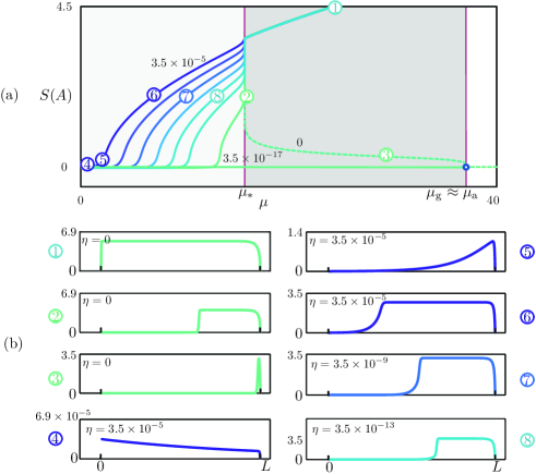
Figure 3: (a) Branches of steady states of Eq. (1.1) for $\alpha=2$, $U=12$, $L=10\pi$, represented using the solution measure $S(A)\equiv-\operatorname{sgn}A^{\prime}(L)\|A\|_{2}$ along the vertical axis, for various inlet boundary conditions $A(0,t)=\eta\in[0,3.5\times 10^{-5}]$ and $A(L,t)=0$. Here the prime denotes differentiation with respect to $x$ and $\|\cdot\|_{2}$ is the standard $L_{2}$ norm. Stable (unstable) branches are indicated via solid (dashed) lines. (b) The solution profiles $A(x)$, $x\in[0,L]$, corresponding to the locations indicated in panel (a). The vertical scale is indicated for each profile separately. The states in $\mu<\mu_{\ast}$ originate in the convective instability of $A=0$, while the states in $\mu>\mu_{\ast}$ are the consequence of absolute instability.

2 Basic properties of the model

In this Section we summarize the basic properties of the model (1.1) on large but finite domains. As already explained the bifurcation parameter $\mu$ controls the stability of the trivial state $A=0$: on the real line, homogeneous solutions grow when $\mu>0$ and saturate at amplitude $\pm\mathchoice{{\hbox{$\displaystyle\sqrt{\mu\,}$}\lower 0.4pt\hbox{\vrule height=4.30554pt,depth=-3.44446pt}}}{{\hbox{$\textstyle\sqrt{\mu\,}$}\lower 0.4pt\hbox{\vrule height=4.30554pt,depth=-3.44446pt}}}{{\hbox{$\scriptstyle\sqrt{\mu\,}$}\lower 0.4pt\hbox{\vrule height=3.01389pt,depth=-2.41113pt}}}{{\hbox{$\scriptscriptstyle\sqrt{\mu\,}$}\lower 0.4pt\hbox{\vrule height=2.15277pt,depth=-1.72223pt}}}$ owing to the nonlinear term $-A^{3}$. When $\alpha=0$ the advection term $UA_{x}$ represents advection of spatial inhomogeneities to the right at speed $U$. As a result near $0<\mu\ll 1$ infinitesimal spatially localized disturbances of $A=0$ travel to the right more rapidly than they grow and at each fixed location the disturbance decays to zero as $t\rightarrow\infty$. Thus, despite the growth of the instability in an appropriately moving frame, the state $A=0$ remains stable in this sense. In the fluid mechanical literature the point $\mu=0$ is referred to as the threshold for convective instability. The term $\alpha>0$ does not change this linear picture but it does imply that the advection speed is reduced as the amplitude of the state grows. Thus nonlinear states are not necessarily advected downstream and can in fact invade the whole domain (Figure 1(b)). In the following we refer to this behavior as nonlinear absolute instability by analogy with the notion of (linear) absolute instability which arises at $\mu=\mu_{\mathrm{a}}:=U^{2}/4$. At this parameter value the growth rate of a localized infinitesimal perturbation of $A=0$ is able to compete for the first time with the rate at which it is swept downstream, i.e., at $\mu=\mu_{\mathrm{a}}$ the upstream spreading speed exactly balances the downstream advection.

In systems of this kind, boundaries play a crucial role: linear theory shows that in the presence of (nonperiodic) boundary conditions that preserve the base state $A=0$, this state loses stability at $\mu_{\mathrm{g}}$, corresponding to the presence of a neutrally stable global eigenmode $A_{\mathrm{g}}(x)$. In domains of large length $L$ one finds that $\mu_{\mathrm{g}}=\mu_{\mathrm{a}}+O(L^{-2})$ [10, 38]. In such domains the threshold of linear instability is thus delayed, by an $O(1)$ amount, from the threshold $\mu=0$ for the onset of instability in the corresponding problem with periodic boundary conditions. Thus for $\mu<\mu_{\mathrm{g}}$ infinitesimal perturbations of $A=0$ decay, albeit on an $O(L)$ time scale, but for $\mu>\mu_{\mathrm{g}}$ they grow. For $\mu=\mu_{\mathrm{g}}+O(L^{-5})$ the solutions of the nonlinear problem resemble the linear theory eigenmode $A_{\mathrm{g}}(x)$ at $\mu=\mu_{\mathrm{g}}$ [10, 38]; this eigenmode is typically compressed against the downstream wall and we call it a wall mode. As $\mu$ increases further, an abrupt transition takes place whereby the domain fills with the $A\neq 0$ state, except for a residual defect near the upstream boundary [38].

The above scenario appears to be typical of systems with broken reflection symmetry, confined in a finite domain, provided the primary bifurcation is supercritical. However, as already mentioned, the system (1.1) is expected to become strongly subcritical when $\alpha$ is sufficiently large (in fact, $\alpha>6/U$ [10]) and this fact suggests that a different domain-filling scenario may take place. Figure 1(a) sketches the typical bifurcation diagram one obtains for $\alpha>6/U$. The figure shows the maximum value of $A$ as a function of $\mu$ and reveals that when $A(0,t)=0$ the branch of global solutions bifurcates subcritically from $\mu=\mu_{\rm g}$ before turning around towards larger values of $\mu$ at a fold located at $\mu=\mu_{\ast}$. For $\mu<\mu_{\ast}$ no steady, i.e., persistent, states of the system exist and all initial perturbations ultimately decay to $A=0$. However, as shown below, as soon as $0<|A(0,t)|\ll 1$, this is no longer the case and a branch of steady states exists throughout $0<\mu<\mu_{\ast}$.

A remarkable fact is that these branches are extremely sensitive to the exact value of the inlet boundary condition $A(0,t)$. We illustrate this fact by explicit computations of steady states of Eq. (1.1) with boundary conditions $A(0,t)=\eta$, $A(L,t)=0$, for moderate values of the advection speed $U$ and $\alpha=2$ (Figure 3). The figure reveals the presence of nonzero steady solutions in $\mu<\mu_{*}$ even for extremely small values of $\eta$ ($3.5\times 10^{-17}\leq\eta\leq 3.5\times 10^{-5}$), together with sample solution profiles at locations indicated in the figure. Unlike Figure 1(a), Figure 3(a) shows the quantity $S(A)\equiv-\operatorname{sgn}A^{\prime}(L)\|A\|_{2}$ as a function of $\mu$, where the prime denotes differentiation with respect to $x$ and $\|\cdot\|_{2}$ is the standard $L_{2}$ norm, and does so for various inlet boundary conditions $\eta\in[0,3.5\times 10^{-5}]$.

The new solution measure unfolds the neighbourhood of $\mu_{\ast}$ for $\eta=0$, revealing a steep vertical branch, along which the position of the front varies continuously (Figure 3(b)). The figure shows that the fold at $\mu=\mu_{\ast}$ on the $\eta=0$ solution branch is in fact highly degenerate and that all the $\eta\neq 0$ branches accumulate on it. It turns out (see below) that the degeneracy is a reflection of an orbit flip in the spatial dynamics description of the system [9], while the existence of the finite amplitude states for $0<\mu<\mu_{\ast}$ is related to canard-like behavior present in this description. We also provide a physical interpretation of the states found for $\mu<\mu_{\ast}$, and relate their properties to the noise-sustained structures present in convectively unstable systems [11].

Both boundary layers and interior layers occurring in singularly perturbed nonlinear BVPs have in fact been studied extensively over many years [7, 14]. In addition, the work by Gorelov and Sobolev [35, 36] analyzes canard solutions to BVPs in ODE models of combustion. A recent review [31] provides an excellent guide to the literature on BVPs with Dirichlet boundary conditions and the connection between such systems and the canard phenomenon, albeit almost exclusively for linear systems. In the present paper we extend this type of discussion not only to strongly nonlinear situations, but also explain how the bifurcation structure associated with canard-type phase plane trajectories affects the temporal dynamics of the PDE, subject to variable inlet boundary conditions. The spatial orbits containing canard segments considered here are in fact transient solutions to the spatial dynamics problem, and so are unrelated to the classical periodic canard cycles of the (forced) van der Pol oscillator, which are asymptotic states.

3 The slow-fast system

In this paper we seek to extend the above results in two directions, to determine the nonlinear states (if any) present in the convectively unstable regime, and to relate these states to the states generated by the subcritical absolute instability at $\mu=\mu_{\rm g}$. For this purpose we consider Eq. (1.1) in the limit of large advection and introduce the small parameter

$$0<\varepsilon=U^{-2}\ll 1.$$

To retain a significant nonlinear contribution to the advection speed we scale the amplitude $A$ as follows, $A=\varepsilon^{-1/4}A^{\prime}$, where by assumption $A^{\prime}=O(1)$, i.e., we focus on appropriately large amplitudes $A$. The diffusion term is retained at leading order provided $x=\varepsilon^{1/2}x^{\prime}$, where $x^{\prime}=O(1)$, i.e., we focus on small spatial scales $x$, of order $\varepsilon^{1/2}$, and hence consider domains of size $L=\varepsilon^{1/2}\ell$, where $\ell$ is formally $O(1)$ but is large compared to the scale on which the front evolves. Time evolution then takes place on an $O(\varepsilon)$ time scale (see Figures 1 and 2), and we therefore write $t=\varepsilon t^{\prime}$, where $t^{\prime}=O(1)$. These scalings all follow from the observation that rapid advection will be balanced by diffusion only on appropriately small spatial scales and that the evolution will then inevitably take place on the short, advective, time scale.

With the above scalings we arrive at the following PDE, dropping primes,

(3.2) $$A_{t}=A_{xx}-(1-\alpha A^{2})A_{x}+\varepsilon\mu A-\mathchoice{{\hbox{$\displaystyle\sqrt{\varepsilon\,}$}\lower 0.4pt\hbox{\vrule height=4.30554pt,depth=-3.44446pt}}}{{\hbox{$\textstyle\sqrt{\varepsilon\,}$}\lower 0.4pt\hbox{\vrule height=4.30554pt,depth=-3.44446pt}}}{{\hbox{$\scriptstyle\sqrt{\varepsilon\,}$}\lower 0.4pt\hbox{\vrule height=3.01389pt,depth=-2.41113pt}}}{{\hbox{$\scriptscriptstyle\sqrt{\varepsilon\,}$}\lower 0.4pt\hbox{\vrule height=2.15277pt,depth=-1.72223pt}}}A^{3},\qquad(x,t)\in(0,\ell)\times(0,\infty).$$

This equation is to be solved subject to the Dirichlet boundary conditions

(3.3) $$A(0,t)=\eta,\qquad A(\ell,t)=0,\qquad t\in[0,\infty),$$

starting from a suitably defined initial condition. The linear stability of steady states $A(x)$ of (3.2) with the boundary conditions (3.3) is determined from the eigenvalues $\lambda$ of the linear problem $\mathcal{L}(A)\psi=\lambda\psi$, where

(3.4) $$\mathcal{L}(A)=\partial^{2}_{x}-(1-\alpha A^{2})\partial_{x}+2\alpha A\partial_{x}A+\varepsilon\mu-3\mathchoice{{\hbox{$\displaystyle\sqrt{\varepsilon\,}$}\lower 0.4pt\hbox{\vrule height=4.30554pt,depth=-3.44446pt}}}{{\hbox{$\textstyle\sqrt{\varepsilon\,}$}\lower 0.4pt\hbox{\vrule height=4.30554pt,depth=-3.44446pt}}}{{\hbox{$\scriptstyle\sqrt{\varepsilon\,}$}\lower 0.4pt\hbox{\vrule height=3.01389pt,depth=-2.41113pt}}}{{\hbox{$\scriptscriptstyle\sqrt{\varepsilon\,}$}\lower 0.4pt\hbox{\vrule height=2.15277pt,depth=-1.72223pt}}}A^{2}$$

and $\psi(0)=\psi(\ell)=0$. Thus when $\lambda<0$ ($\lambda>0$) the solution $A(x)$ is stable (unstable) in time. Since translation invariance is absent, there is no zero eigenvalue. Henceforth we work exclusively with the rescaled model, and therefore present numerical results for Eqs. (3.2)–(3.3), or equivalently for the corresponding spatial-dynamical system, introduced in Section 4 below.

4 Bifurcation diagram for the system (3.2)–(3.3)

In this section we employ a spatial dynamics formulation of the steady state BVP and use it to construct a variety of different solutions that together comprise the bifurcation diagram. The analysis explains not only the behavior shown in Figure 3 but reveals in addition a multitude of other solution types whose origin is confirmed by numerical solution of the time-dependent BVP (3.2)–(3.3).

4.1 The spatial van der Pol oscillator

It is advantageous to interpret the steady state problem associated with (1.1) as a second-order van der Pol equation with independent variable $x$. We refer to the resulting system as a spatial van der Pol oscillator. We set $z_{1}=A$ and use the Liénard transformation $z_{2}=-A^{\prime}+A-(\alpha/3)A^{3}$ to obtain the first-order BVP

(4.5) $$z^{\prime}_{1}=-z_{2}+z_{1}-\frac{\alpha}{3}z_{1}^{3}$$

(4.6) $$z^{\prime}_{2}=\mathchoice{{\hbox{$\displaystyle\sqrt{\varepsilon\,}$}\lower 0.4pt\hbox{\vrule height=4.30554pt,depth=-3.44446pt}}}{{\hbox{$\textstyle\sqrt{\varepsilon\,}$}\lower 0.4pt\hbox{\vrule height=4.30554pt,depth=-3.44446pt}}}{{\hbox{$\scriptstyle\sqrt{\varepsilon\,}$}\lower 0.4pt\hbox{\vrule height=3.01389pt,depth=-2.41113pt}}}{{\hbox{$\scriptscriptstyle\sqrt{\varepsilon\,}$}\lower 0.4pt\hbox{\vrule height=2.15277pt,depth=-1.72223pt}}}(\mathchoice{{\hbox{$\displaystyle\sqrt{\varepsilon\,}$}\lower 0.4pt\hbox{\vrule height=4.30554pt,depth=-3.44446pt}}}{{\hbox{$\textstyle\sqrt{\varepsilon\,}$}\lower 0.4pt\hbox{\vrule height=4.30554pt,depth=-3.44446pt}}}{{\hbox{$\scriptstyle\sqrt{\varepsilon\,}$}\lower 0.4pt\hbox{\vrule height=3.01389pt,depth=-2.41113pt}}}{{\hbox{$\scriptscriptstyle\sqrt{\varepsilon\,}$}\lower 0.4pt\hbox{\vrule height=2.15277pt,depth=-1.72223pt}}}\mu z_{1}-z_{1}^{3})$$

(4.7) $$z_{1}(0)=\eta,\quad z_{1}(\ell)=0.$$

We identify steady states of Eqs. (3.2)–(3.3) with solutions to the two-point BVP (4.5)–(4.7) and use its slow-fast structure to interpret the solution branches shown in Figure 3. To this end, we temporarily depart from the corresponding PDE formulation and represent the solutions of the time-independent BVP (3.2)–(3.3) in the spatial phase plane. For this purpose we use the term spatial stability or simply stability to classify the asymptotic behavior of stationary solutions to (4.5)–(4.6). The PDE stability of the corresponding steady states is determined by solving the eigenvalue problem (3.4), as described in Section 3.

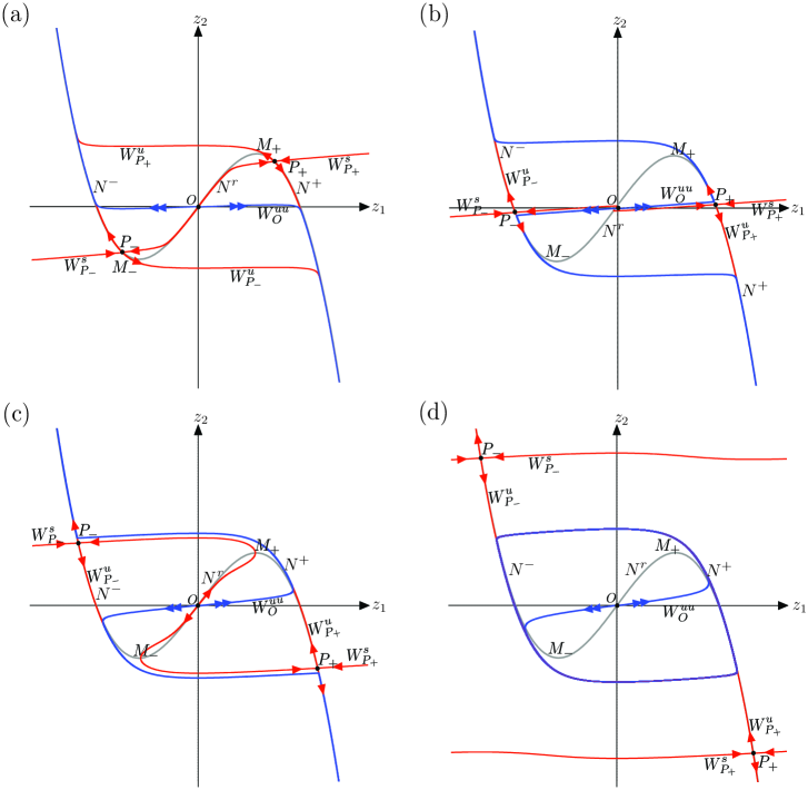
Figure 4: Phase planes for Eqs. (4.5)–(4.6) when $\varepsilon=1/144$, $\alpha=5$, and (a) $\mu=4$, (b) $\mu=7$, (c) $\mu=10$, (d) $\mu=13$. The phase planes are representative of spatial dynamics in sectors 1–3: (a) sector 1 ($0<\mu<\mu_{*}$), (b) in sector 2 ($\mu_{*}<\mu<\mu_{c+}$), close to the transition between 1 and 2, (c) in sector 2 ($\mu_{*}<\mu<\mu_{c+}$), close to the transition between 2 and 3, (d) in sector 3 ($\mu>\mu_{c+}$). For description and definition of $\mu_{c+}$ see Figure 12 and Appendix A.

Figure 4 shows the phase plane for this system and various values of the principal bifurcation parameter $\mu$, with $z_{1}$ plotted horizontally and $z_{2}$ vertically. Each panel shows the fast nullcline $N:=N^{-}\cup N^{r}\cup N^{+}$, usually referred to as the critical manifold of the slow-fast system,

(4.8) $$z_{2}=z_{1}-\frac{\alpha}{3}z_{1}^{3},$$

together with the line $z_{1}=0$ along which $z^{\prime}_{2}=0$. The critical manifold is divided into three branches, two (outer) attracting branches $N^{\pm}$ and one (middle) repelling branch $N^{r}$. There are three fixed points, one at the origin $O:(z_{1},z_{2})=(0,0)$ and the others at $P_{\pm}:(z_{1},z_{2})=\pm(\varepsilon^{1/4}\mathchoice{{\hbox{$\displaystyle\sqrt{\mu\,}$}\lower 0.4pt\hbox{\vrule height=4.30554pt,depth=-3.44446pt}}}{{\hbox{$\textstyle\sqrt{\mu\,}$}\lower 0.4pt\hbox{\vrule height=4.30554pt,depth=-3.44446pt}}}{{\hbox{$\scriptstyle\sqrt{\mu\,}$}\lower 0.4pt\hbox{\vrule height=3.01389pt,depth=-2.41113pt}}}{{\hbox{$\scriptscriptstyle\sqrt{\mu\,}$}\lower 0.4pt\hbox{\vrule height=2.15277pt,depth=-1.72223pt}}},\varepsilon^{1/4}\mathchoice{{\hbox{$\displaystyle\sqrt{\mu\,}$}\lower 0.4pt\hbox{\vrule height=4.30554pt,depth=-3.44446pt}}}{{\hbox{$\textstyle\sqrt{\mu\,}$}\lower 0.4pt\hbox{\vrule height=4.30554pt,depth=-3.44446pt}}}{{\hbox{$\scriptstyle\sqrt{\mu\,}$}\lower 0.4pt\hbox{\vrule height=3.01389pt,depth=-2.41113pt}}}{{\hbox{$\scriptscriptstyle\sqrt{\mu\,}$}\lower 0.4pt\hbox{\vrule height=2.15277pt,depth=-1.72223pt}}}[1-(\alpha/3)\varepsilon^{1/2}\mu])$. The former is unstable with eigenvalues $\lambda=(1/2)[1\pm\mathchoice{{\hbox{$\displaystyle\sqrt{1-4\varepsilon\mu\,}$}\lower 0.4pt\hbox{\vrule height=6.44444pt,depth=-5.15558pt}}}{{\hbox{$\textstyle\sqrt{1-4\varepsilon\mu\,}$}\lower 0.4pt\hbox{\vrule height=6.44444pt,depth=-5.15558pt}}}{{\hbox{$\scriptstyle\sqrt{1-4\varepsilon\mu\,}$}\lower 0.4pt\hbox{\vrule height=4.51111pt,depth=-3.6089pt}}}{{\hbox{$\scriptscriptstyle\sqrt{1-4\varepsilon\mu\,}$}\lower 0.4pt\hbox{\vrule height=3.22221pt,depth=-2.57779pt}}}]\approx 1,\varepsilon\mu$, while the latter are always saddles. The eigenvalues of $O$ are real if $\mu<1/(4\varepsilon)$ but complex if $\mu>1/(4\varepsilon)$. The equality $\mu=1/(4\varepsilon)$ defines the onset of absolute instability, i.e., $\mu=\mu_{\mathrm{a}}$. This is because the linearized two-point BVP with the boundary conditions $A(0)=A(\ell)=0$, or equivalently

(4.9) $$z_{1}(0)=z_{1}(\ell)=0,$$

only has solutions when the spatial eigenvalues are complex but not otherwise. Note that in the vicinity of this point the slow-fast decomposition necessarily fails. However, since this point moves off to infinity in the limit of interest, $\varepsilon\to 0$, this issue does not arise when studying solutions for $\mu=O(1/\mathchoice{{\hbox{$\displaystyle\sqrt{\varepsilon\,}$}\lower 0.4pt\hbox{\vrule height=4.30554pt,depth=-3.44446pt}}}{{\hbox{$\textstyle\sqrt{\varepsilon\,}$}\lower 0.4pt\hbox{\vrule height=4.30554pt,depth=-3.44446pt}}}{{\hbox{$\scriptstyle\sqrt{\varepsilon\,}$}\lower 0.4pt\hbox{\vrule height=3.01389pt,depth=-2.41113pt}}}{{\hbox{$\scriptscriptstyle\sqrt{\varepsilon\,}$}\lower 0.4pt\hbox{\vrule height=2.15277pt,depth=-1.72223pt}}})$ or less.

Figure 4 shows that the critical manifold $N$ has a pair of turning points $M_{\pm}:(z_{1},z_{2})=\pm(1/\mathchoice{{\hbox{$\displaystyle\sqrt{\alpha\,}$}\lower 0.4pt\hbox{\vrule height=4.30554pt,depth=-3.44446pt}}}{{\hbox{$\textstyle\sqrt{\alpha\,}$}\lower 0.4pt\hbox{\vrule height=4.30554pt,depth=-3.44446pt}}}{{\hbox{$\scriptstyle\sqrt{\alpha\,}$}\lower 0.4pt\hbox{\vrule height=3.01389pt,depth=-2.41113pt}}}{{\hbox{$\scriptscriptstyle\sqrt{\alpha\,}$}\lower 0.4pt\hbox{\vrule height=2.15277pt,depth=-1.72223pt}}},2/3\mathchoice{{\hbox{$\displaystyle\sqrt{\alpha\,}$}\lower 0.4pt\hbox{\vrule height=4.30554pt,depth=-3.44446pt}}}{{\hbox{$\textstyle\sqrt{\alpha\,}$}\lower 0.4pt\hbox{\vrule height=4.30554pt,depth=-3.44446pt}}}{{\hbox{$\scriptstyle\sqrt{\alpha\,}$}\lower 0.4pt\hbox{\vrule height=3.01389pt,depth=-2.41113pt}}}{{\hbox{$\scriptscriptstyle\sqrt{\alpha\,}$}\lower 0.4pt\hbox{\vrule height=2.15277pt,depth=-1.72223pt}}})$. Owing to symmetry, in the following we only consider the saddle $P_{+}$ and its position on $N$ relative to $M_{+}$. We find that for $\mu<1/(\alpha\mathchoice{{\hbox{$\displaystyle\sqrt{\varepsilon\,}$}\lower 0.4pt\hbox{\vrule height=4.30554pt,depth=-3.44446pt}}}{{\hbox{$\textstyle\sqrt{\varepsilon\,}$}\lower 0.4pt\hbox{\vrule height=4.30554pt,depth=-3.44446pt}}}{{\hbox{$\scriptstyle\sqrt{\varepsilon\,}$}\lower 0.4pt\hbox{\vrule height=3.01389pt,depth=-2.41113pt}}}{{\hbox{$\scriptscriptstyle\sqrt{\varepsilon\,}$}\lower 0.4pt\hbox{\vrule height=2.15277pt,depth=-1.72223pt}}})$ the point $P_{+}$ lies between $O$ and $M_{+}$ while for $\mu>1/(\alpha\mathchoice{{\hbox{$\displaystyle\sqrt{\varepsilon\,}$}\lower 0.4pt\hbox{\vrule height=4.30554pt,depth=-3.44446pt}}}{{\hbox{$\textstyle\sqrt{\varepsilon\,}$}\lower 0.4pt\hbox{\vrule height=4.30554pt,depth=-3.44446pt}}}{{\hbox{$\scriptstyle\sqrt{\varepsilon\,}$}\lower 0.4pt\hbox{\vrule height=3.01389pt,depth=-2.41113pt}}}{{\hbox{$\scriptscriptstyle\sqrt{\varepsilon\,}$}\lower 0.4pt\hbox{\vrule height=2.15277pt,depth=-1.72223pt}}})$ it lies past $M_{+}$. In the former case $P_{+}$ is attracting along $N$ ($M_{+}$ is repelling along $N$) while in the latter case it is repelling ($M_{+}$ is attracting along $N$; see Figure 4). Moreover, the middle part $N^{r}$ of $N$ is repelling in the $z_{1}$ direction while that beyond $M_{+}$, $N^{+}$, is attracting. We also observe that $P_{+}$ lies on the axis $z_{2}=0$ when $\mu=(3/\alpha)\varepsilon^{-1/2}$. These results suffice to construct the flow of the system in the $(z_{1},z_{2})$ plane. Figure 4 shows the resulting phase plane computed for $\varepsilon=1/144$, $\alpha=5$ and several different values of the bifurcation parameter $\mu$. Note in particular that panel (a) for $\mu=4$ and panel (c) for $\mu=10$ both show that for certain values of $\mu$ the position of the saddle equilibria $P_{\pm}$ is such that their stable manifold connects (in backward ’time’) to the origin following the middle branch $N^{r}$ of $N$. As we shall see in the rest of the paper, this allows for solutions of the BVP (4.5)–(4.7) for $\eta\neq 0$ that also follow $N^{r}$. Such solutions thus contain canard segments; see Appendix A for details.

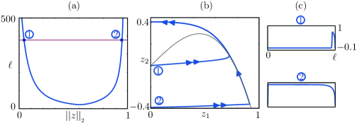
Figure 5: (a) Solution branch of Eqs. (4.5)–(4.7) with $\eta=0$, obtained by varying $\ell$ for $\varepsilon=1/144$, $\alpha=5$ and $\mu=10$. Two solutions are found for $\ell=377$ (straight line), and these are shown as trajectories in the spatial phase plane $(z_{1},z_{2})$ (panel (b)) and as space-dependent stationary states $A(x)$ of the PDE (3.2)–(3.3) with $\eta=0$ (panel (c)).

We now describe the solution of the BVP (4.9), i.e., the original BVP of [9, 10], using the qualitative information contained in Figure 4. We assume that $z_{1}(x)>0$ for $x\in(0,\ell)$. Such solutions exist only if $z_{2}(0)<0$. For suppose that $z_{2}(0)>0$. Then $z^{\prime}_{1}$ at $z_{1}=0$ is strictly negative, so that the flow enters immediately into the negative half plane. Hence solutions of this BVP can exist only if $z_{2}(0)<0$. We now argue that such solutions do not exist if $\mu$ is too small. The critical value of $\mu$ is determined by the so-called orbit flip bifurcation at which a branch of $W^{s}(P_{+})$ coincides with the strong unstable manifold of $O$, denoted by $W^{uu}(O)$. As shown by Couairon & Chomaz [9] this occurs when $\mu=\mu_{\ast}=3\alpha^{-1}(U-3\alpha^{-1})\approx 3/(\alpha\mathchoice{{\hbox{$\displaystyle\sqrt{\varepsilon\,}$}\lower 0.4pt\hbox{\vrule height=4.30554pt,depth=-3.44446pt}}}{{\hbox{$\textstyle\sqrt{\varepsilon\,}$}\lower 0.4pt\hbox{\vrule height=4.30554pt,depth=-3.44446pt}}}{{\hbox{$\scriptstyle\sqrt{\varepsilon\,}$}\lower 0.4pt\hbox{\vrule height=3.01389pt,depth=-2.41113pt}}}{{\hbox{$\scriptscriptstyle\sqrt{\varepsilon\,}$}\lower 0.4pt\hbox{\vrule height=2.15277pt,depth=-1.72223pt}}})$. For $\mu>\mu_{\ast}$ the separatrix $W^{s}(P_{+})$ must be below $W^{uu}(O)$. Hence, continued backwards in ‘time’, it must intersect the $z_{2}$ axis at some $z_{2,s}<0$. It follows that for each $z_{2}\in(z_{2,s},0)$ there exists $\ell>0$ such that the BVP (4.9) has a solution with this choice of $\ell$ and $z_{2}(0)=z_{2}$. Note that $\ell\to\infty$ both as $z_{2}(0)$ tends to $0$ and to $z_{2,s}$ (Figure 5). It follows that for $\ell$ large enough there exist at least two solutions of (4.9) for the same $\ell$, one with $z_{2}$ close to $0$ and one with $z_{2}$ close to $z_{2,s}$. The solution with $z_{2}(0)\approx 0$ spends a long ‘time’ near $O$ since $O$ is a fixed point, which implies that its $L_{2}$ norm is small. The solution starting near $z_{2,s}$ spends a long ‘time’ near $P_{+}$ for the same reason and its $L_{2}$ norm is therefore large. As $\mu$ approaches $\mu_{\ast}$ from above these two solutions approach each other and the solution with the small $L_{2}$ norm develops a longer segment near $P_{+}$, implying rapid growth of the $L_{2}$ norm. Hence the quasi-vertical segment of the solution branch near $\mu=\mu_{\ast}$ (Figure 3(a)) is due to an orbit flip.

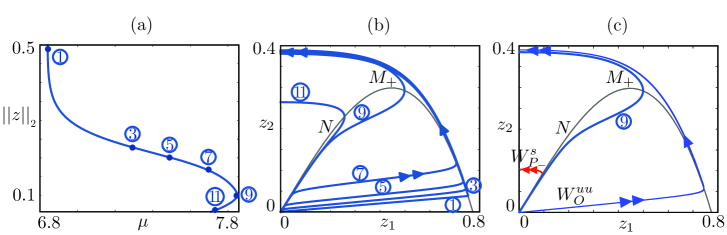
Figure 6: (a) Detail of the small amplitude convective instability branch computed from (4.5)–(4.7) with $\alpha=5$, $\varepsilon=1/144$ and $\eta=10^{-10}$. (b) Portion of the phase plane showing the trajectories corresponding to the points indicated in (a). (c) Trajectory 9 from (a) and (b), displaying a canard segment, together with some of the invariant manifolds of equilibria of the system present at this value of $\mu$. The point $P_{+}$ lies below the $z_{1}$ axis. Figure 12(a) provides are larger view of this case.

For comparison we show in Figure 6 the corresponding results for

(4.10) $$z_{1}(0)=\eta,\qquad z_{1}(\ell)=0$$

with $\eta=10^{-10}$. The figure corresponds to sector 2 (panels (b) and (c) in Figure 4) and reveals the appearance of a new fold in the solution branch (Figure 6(a)). This fold is visible here because of the larger value of $\alpha$ used; such a fold is present for $\alpha=2$ also but only for even smaller values of $\eta$ than those used in generating Figure 3. The phase portraits corresponding to the locations 1–11 on the branch in Figure 6(a) are shown in Figure 6(b). Of particular interest in this paper are trajectories resembling trajectory 9 (Figure 6(c)) which follows for a ’time’ the repelling manifold $N^{r}$ before reaching $z_{1}=0$ at a finite value of $z_{2}$. These trajectories are associated with the canard phenomenon and are discussed in detail in Appendix A.

4.2 Solution profiles

Figure 3(b) compares the solution profiles along the convective and absolute instability branches for $\alpha=2$, starting with the profiles 1–3 along the absolute instability branch. These solutions can be computed for $\eta=0$ since they are insensitive to the precise value of $\eta$. The location of the solutions on the branch is indicated in Figure 3(a). Profile 3 shows a solution that is strongly compressed against the downstream boundary; this solution resembles the neutral wall mode predicted by linear stability theory for the state $A\equiv 0$. Decreasing $\mu$ leads to an increase in the amplitude of the solution (Figure 3(a)); at the same time the solution broadens and starts to fill the domain. Profile 2 corresponds to $\mu=\mu_{\ast}$ and is located in the region of abrupt amplitude growth associated with the orbit flip. We see that the solution develops a plateau corresponding to $A=\mathchoice{{\hbox{$\displaystyle\sqrt{\mu_{\ast}\,}$}\lower 0.4pt\hbox{\vrule height=4.30554pt,depth=-3.44446pt}}}{{\hbox{$\textstyle\sqrt{\mu_{\ast}\,}$}\lower 0.4pt\hbox{\vrule height=4.30554pt,depth=-3.44446pt}}}{{\hbox{$\scriptstyle\sqrt{\mu_{\ast}\,}$}\lower 0.4pt\hbox{\vrule height=3.01389pt,depth=-2.41113pt}}}{{\hbox{$\scriptscriptstyle\sqrt{\mu_{\ast}\,}$}\lower 0.4pt\hbox{\vrule height=2.15277pt,depth=-1.72223pt}}}$ and that the length of this plateau increases as the solution norm increases. The shape of the front connecting this plateau to $A=0$ remains fixed but the location of the front migrates very rapidly upstream. This process terminates when the front reaches the upstream boundary and so becomes pinned at a particular location. Subsequent to this pinning event the branch turns around to larger values of $\mu$ and the amplitude of the plateau grows in proportion to $\textstyle\sqrt{\mu\,}$  (profile 1).

Profiles 4–8 in Figure 3(b) are instead selected from the convective instability branches. Profiles 4–6 show the evolution of the solution with increasing $\mu$ when $\eta=10^{-5}$. Near $\mu=0$ the solution decreases from $\eta=10^{-5}$ at $x=0$ towards $A=0$ at $x=\ell$. The slope is almost constant throughout the domain, indicating a balance between $UA_{x}$ and $\mu A$ with small adjustment near the downstream boundary (profile 4). As $\mu$ increases the slope reverses, with the amplitude growing towards the downstream boundary (profile 5). As $\mu$ increases further the amplitude near the downstream boundary saturates and the solution develops a plateau that evolves in a similar fashion to that on the absolute instability branch with increasing $\mu$ (profile 6). Profiles 7 and 8 correspond to branches with yet smaller $\eta$ ($\eta=10^{-9}$ and $10^{-13}$, respectively); since decreasing $\eta$ delays the onset of spatial growth the solutions reach a given norm at larger $\mu$ and hence with a higher amplitude of the plateau. For yet smaller values of $\eta$ (not shown) one find the behavior shown in Figure 6(a) with an additional fold at $\mu=\mu_{\eta}$.

4.3 Stability in time

A standard PDE stability calculation [39] shows that the convective instability branches are stable in time throughout their range of existence when the fold at $\mu=\mu_{\eta}$ is absent, and stable in $0<\mu<\mu_{\eta}$ when the fold $\mu_{\eta}$ is present. In the former case stability is transferred at the degenerate fold to the upper part of the absolute instability branch; this branch is also stable. In the latter case there is a hysteretic transition to the upper absolute instability branch at $\mu=\mu_{\eta}$. Thus a stable steady solution is in fact present for all $\mu>0$ provided only that $A(0)\neq 0$ (Figure 3).

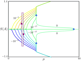
Figure 7: Branches of steady states of Eq. (3.2) with $\alpha\!=\!2$ and various inlet boundary conditions $\eta\in[-10^{-5},10^{-5}]$ with a superposed cycle (in red) showing changes in the solution amplitude when $\eta$ oscillates quasistatically in time with $O(10^{-5})$ amplitude and mean $\eta=0$. A concrete example is shown in Figure 8.

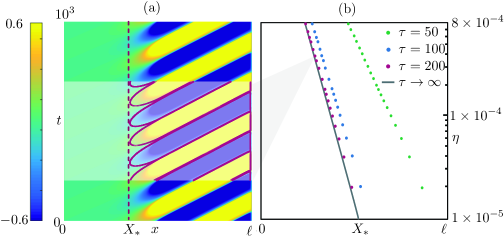
Figure 8: (a) Location $X_{*}$ from Eq. (5.11) of time-periodic fronts when Eq. (3.2) is subjected to a time-periodic inlet boundary condition $A(0,t)=\eta\sin(2\pi t/\tau)$; such fronts are sustained entirely by the small amplitude modulation in $A(0,t)$ (in the example shown here $\mu=6.1$, $\eta=4\times 10^{-4}$, $\tau=200$, with the other parameters as in Figure 7). The red lines in the central part are the contour lines $A(x,t)=\pm 0.1$. (b) The front location $X_{*}$ for various values $\eta$ and $\tau$ (dots). The steady states of Figure 7 are continued at $\mu=6.07$ in the parameter $\eta$. These states have a well-defined front location, so we use the resulting $X_{*}$ as a solution measure (curve marked $\tau\to\infty$). The large $\tau$ time-periodic simulations are well approximated by the steady-state continuation.

5 PDE simulations

Given the sensitivity of the system to the inlet boundary condition $A(0,t)=\eta$, a question arises as to how solutions behave when this parameter is time-dependent or randomly distributed.

5.1 Time-dependent inlet boundary condition

Figure 7 presents the solution branches computed from Eq. (3.2) with $\alpha=2$ and different values of the inlet amplitude $\eta$. The results are similar to those presented in the previous sections for $\alpha=5$: as $\eta$ varies within an $O(10^{-5})$ interval of $\eta=0$ the front location in the corresponding steady states changes dramatically, as witnessed by the $O(1)$ variations in the solution measure $S(A)$.

We now fix $\mu$ at a value below $\mu_{*}$ and prescribe time-periodic inlet boundary conditions, $A(0,t)=\eta\sin(2\pi t/\tau)$. As sketched in Figure 7, for fixed $\mu$ and sufficiently large $\tau$ we expect the front location to oscillate as the spatio-temporal solution drifts from one branch of stable stationary states to the next and back again.

In Figure 8(a) we present a numerical experiment for $\mu=6.07$ with a slowly-varying, small-amplitude inlet condition ($\eta=4\times 10^{-4}$, $\tau=200$). As expected, a time-periodic front establishes towards the center of the domain; we remark that this front is sustained solely by the small periodic variations in the inlet boundary conditions: if $\eta=0$ the only attractive state in this region of parameter space is the trivial state $A=0$, as seen in Figure 7.

In order to quantify the position of the front, we monitor the level sets of $A(x,t)$ as $t$ varies. In Figure 7 we define this position to be

(5.11) $$X_{*}=\min_{t\in[0,T]}\{x\in[0,\ell]\colon|A(x,t)|=0.1\}.$$

We expect the steady state analysis presented in the previous section to provide information about the front location, and this is confirmed by the results in Figure 8. For solutions with a nonoscillatory profile, such as those considered here, we expect the results to be robust with respect to changes in the threshold value. The figure shows the results of steady state continuation in the parameter $\eta$, using $X_{*}$ as a solution measure (curve labeled $\tau\to\infty$ in Figure 8(b)): the solutions on this branch are steady states, but they have a well-defined $X_{*}$ which approximates the location of time-periodic fronts like that in Figure 8(a). We repeated the direct numerical simulations for various values of $\eta$ and $\tau$, and found that the steady-state approximation is excellent for sufficiently slow oscillations of the inlet boundary conditions (Figure 8(b), $\tau=200$). However, for faster oscillations (Figure 8(b), $\tau=50$, $100$) the dependence of $X_{*}$ on $\eta$ remains logarithmic but with a shallower slope that depends on $\tau$.

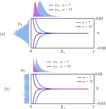
Figure 9: For randomly distributed inlet boundary conditions $\eta$ with density $p_{\eta}$, the location $X_{*}$ of the front in problem (5.12) is distributed with induced density $p_{X_{*}}$. Since for each sample there is a deterministic relation between $\eta$ and $X_{*}$ (the blue and red branches $X_{*}(\eta)$), we infer the density $p_{X_{*}}$ directly from $X_{*}(\eta)$ (upper panels). (a) If $p_{\eta}=\mathcal{N}(0,0.01)$, then $X_{*}$ is approximately Beta-distributed; we observe $\mathbb{E}[X_{*}]\to 0$, $\operatorname{var}[X_{*}]\to 0$ as $\mu\to\mu_{\ast}$, i.e., the distribution of front locations moves towards the inlet as $\mu$ increases towards $\mu_{\ast}$. (b) The experiment is repeated, with qualitatively similar results, for $p_{\eta}=\mathcal{U}(-0.03,0.03)$. The distribution $p_{X_{*}}$ is now approximately exponential. Parameters are as in Figure 7.

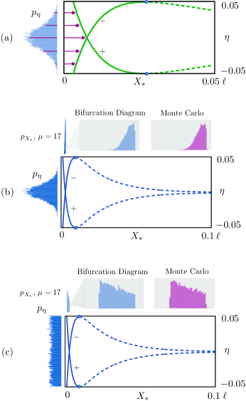
Figure 10: As for Figure 9 but repeated for $\mu=17>\mu_{\ast}$. (a) At this value of $\mu$ the deterministic system possesses two stable solutions that depend on the inlet amplitude $\eta$. We label these solutions using the symbols $-$ and $+$ according to $A(X_{*})>0$ and $A(X_{*})<0$, respectively. These solutions remain stable (solid lines) up to a maximum value of $\eta$ and are unstable beyond (dashed lines). Since $S(A(x,0,\omega))\approx 0$, we expect that the system (5.12) will evolve towards $X^{+}_{*}$ when $\eta(\omega)>0$, and towards $X^{-}_{*}$ when $\eta(\omega)<0$, as indicated by the arrows. (b), (c) The hypothesis of panel (a) is used to approximate $p_{X_{*}}$ (upper panels); for $\mu=17$ the front is located very close to the inlet, and the histograms compare favorably with Monte Carlo simulations of (5.12) with $T=10^{3}$ and $10^{4}$ samples.

5.2 Uncertainty quantification of the front location

Motivated by the discussion in the previous sections, we consider steady states of the problem

(5.12) $$A_{t}=A_{xx}-(1-\alpha A^{2})A_{x}+\varepsilon\mu A-\mathchoice{{\hbox{$\displaystyle\sqrt{\varepsilon\,}$}\lower 0.4pt\hbox{\vrule height=4.30554pt,depth=-3.44446pt}}}{{\hbox{$\textstyle\sqrt{\varepsilon\,}$}\lower 0.4pt\hbox{\vrule height=4.30554pt,depth=-3.44446pt}}}{{\hbox{$\scriptstyle\sqrt{\varepsilon\,}$}\lower 0.4pt\hbox{\vrule height=3.01389pt,depth=-2.41113pt}}}{{\hbox{$\scriptscriptstyle\sqrt{\varepsilon\,}$}\lower 0.4pt\hbox{\vrule height=2.15277pt,depth=-1.72223pt}}}A^{3}, (x,t)\in(0,\ell)\times(0,T),$$

$$A(0,t,\omega)=\eta(\omega),\quad A(\ell,t,\omega)=0, t\in[0,T],$$

$$A(x,0,\omega)=(1-x/\ell)\eta(\omega), x\in[0,\ell],$$

where the random inlet parameter $\eta(\omega)\colon\Omega\to\mathbb{R}$ has an associated density $p_{\eta}$. In what follows, we will choose $p_{\eta}$ so as to give samples $|\eta|\ll 1$, that is, we prescribe small random inlet boundary conditions and study the propagation of uncertainty in the front location $X_{*}$ of steady states attained from approximately flat initial conditions (note that the slope of the initial condition in (5.12) is negligible, since $|\eta|\ll 1$ and $\ell\gg 1$).

Once again, the bifurcation diagrams of Figure 7 help us to understand the problem. We start by fixing $\mu<\mu_{\ast}=15.75$. For a fixed event $\omega\in\Omega$, there is a single attracting steady state $A(x,\omega)$ with a front at $x=X_{*}$ that satisfies $|A(X_{*}(\omega),\omega)|=0.1$. Moreover, for fixed $\omega\in\Omega$, the random variable $X_{*}$ is a deterministic function of $\eta$: the graph of such a function is approximated by the curve labeled $\tau\to\infty$ in Figure 8(b). This means that we can infer directly the density $p_{X_{*}}$ using $p_{\eta}$ and the bifurcation diagram. In Figure 9(a) we use numerical continuation to compute $X_{*}(\eta)$ in the interval $\eta\in[-0.03,0.03]$ for $\mu=7,12<\mu_{\ast}$; we then prescribe a normally distributed inlet boundary condition $p_{\eta}=\mathcal{N}(0,0.01)$ and compute the corresponding densities $p_{X_{*}}$.

The histograms for $p_{X_{*}}$, obtained using $10^{4}$ samples, show that the distribution of the front locations is shifted towards the inlet; we observe, in addition, that $p_{X_{*}}$ resembles a Beta distribution with $\mathbb{E}[X_{*}]\to 0$, $\operatorname{var}[X_{*}]\to 0$ as $\mu\to\mu_{\ast}$. Consequently, the uncertainty in the front location decreases considerably as we transition towards $\mu_{\ast}$: for $\mu=7$, some samples have fronts close to $\ell/2$, as can be seen in the blue histogram of Figure 9(a), while the distribution for $\mu=12$ peaks much closer to the inlet. In Figure 9(b) we repeat the calculations for uniformly distributed inlet boundary conditions, $p_{\eta}=\mathcal{U}(-0.03,0.03)$. The results are qualitatively similar to the normally distributed case, except that $p_{X_{*}}$ is now approximated by an exponential distribution.

A complication arises when we consider the case $\mu>\mu_{\ast}=15.7$. In this region of parameter space more than one attracting steady state may be present for each fixed event $\omega$. We have not shown such branches in Figure 7, but refer the reader to Section 6, Figure 12(a), for an example.

Figure 10 shows the results for $\mu=17>\mu_{\ast}$, i.e., in a region of parameter space where two stable solutions with different $X_{*}$ coexist. Both branches are initially stable (solid lines) and destabilize at saddle-node bifurcations; importantly, there are two stable attracting steady states for each $\eta\in[-0.05,0.05]$, selected by the initial conditions for the problem (5.12). Since $S(A(x,0,\omega))\approx 0$, it is reasonable to expect that the system will be attracted to a solution on the branch with $A(X_{*})>0$ when $\eta(\omega)<0$ (labeled $-$), and to a solution on the branch with $A(X_{*})<0$ when $\eta(\omega)>0$ (labeled $+$), as sketched in Figure 10(a). In passing, we note that the $X_{*}$ scale in Figure 10(a) indicates that the front location is much closer to the inlet, $X_{*}\in[0,0.05\ell]$, for $\mu>\mu_{\ast}$ than when $\mu<\mu_{\ast}$ (cf. Figure 9).

The above conjecture is supported by the numerical experiments reported in Figures 10(b,c). We repeated the procedure of Figure 9 for $\mu=17$ assuming that

$$X_{*}(\eta)=\begin{cases}X^{+}_{*}(\eta)&\text{if $\eta<0$,}\\ X^{-}_{*}(\eta)&\text{if $\eta\geq 0$}\end{cases}$$

and found that the resulting densities $p_{X_{*}}$ are sharply peaked around the inlet (upper panels in (b,c)). The insets show an excellent agreement with the histograms computed via Monte Carlo simulations of the system (5.12) using $T=10^{3}$ and $10^{4}$ samples.

5.3 Stochastic simulations

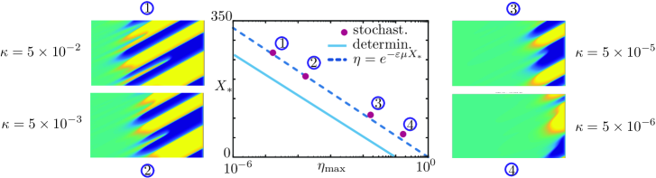
Figure 11: Direct numerical simulations of Eq. (3.2) with a stochastic inlet boundary condition $A(0,t)=\kappa\tilde{\eta}(t)$, where $\kappa>0$ and $\tilde{\eta}(t)$ is a Wiener process (see Eq. (5.13)). We show contour plots of $A(x,t)$ for $(x,t)\in[0,377]\times[0,500]$ for $\mu=6$, $\varepsilon=1/144$ and various values of $\kappa$ (panels 1–4). When $\kappa=0$ the problem is deterministic and the only attracting solution is the trivial steady state $A\equiv 0$ but, as the noise is turned on ($\kappa>0$), noise-sustained structures appear. As $\kappa$ increases so does the maximum inlet amplitude $\eta_{\mathrm{max}}=\max_{t}|\eta(t)|$, resulting in decreased distance $X_{*}$ to the noise-sustained front. The deterministic and stochastic setting have a common scaling $\eta=e^{-\varepsilon\mu X_{*}}$ (see text).

We report, finally, on the results of stochastic simulations in which the inlet value is a continuous stochastic process. Specifically, we set $A(0,t)=\eta(t)=\kappa\tilde{\eta}(t)$, where $\kappa>0$ and $\tilde{\eta}(t)$ is a Wiener process, i.e.,

(5.13) $$\tilde{\eta}(0)=0\text{ a.s, }\qquad\tilde{\eta}(t+s)-\tilde{\eta}(t)\stackrel{{\scriptstyle\text{i.i.d.}}}{{\sim}}\mathchoice{{\hbox{$\displaystyle\sqrt{s\,}$}\lower 0.4pt\hbox{\vrule height=4.30554pt,depth=-3.44446pt}}}{{\hbox{$\textstyle\sqrt{s\,}$}\lower 0.4pt\hbox{\vrule height=4.30554pt,depth=-3.44446pt}}}{{\hbox{$\scriptstyle\sqrt{s\,}$}\lower 0.4pt\hbox{\vrule height=3.01389pt,depth=-2.41113pt}}}{{\hbox{$\scriptscriptstyle\sqrt{s\,}$}\lower 0.4pt\hbox{\vrule height=2.15277pt,depth=-1.72223pt}}}\,\mathcal{N}_{0,1},\quad\text{for all $t,s>0$}.$$

In the following we use the standard Euler-Maruyama scheme [27] to integrate the resulting stochastic PDE. The results in Figure 11 demonstrate the presence of noise-sustained structures in the regime $0<\mu<\mu_{\ast}$, thereby generalizing the results for fixed but randomly selected values of $\eta$ in Section 55.2 and those for periodically oscillating inlet boundary conditions in Section 55.1. Since the only source of randomness is in the boundary condition $A(0,t)=\kappa\eta(t)$, by setting $\kappa=0$ we recover the deterministic system with $0<\mu<\mu_{*}$ and $A(0,t)=0$ for all $t$. The only attracting solution of this system is the trivial steady state $A=0$. As the noise is turned on, noise-sustained structures appear, echoing the behavior found for random but time-independent inlet conditions (Figure 8(b)). In order to make a quantitative comparison with the deterministic case, we compute $X_{*}$ using the definition (5.11) and plot this value against $\eta_{\textrm{max}}=\max_{t}|\eta(t)|$ for each of the realizations reported in Figure 11. Here $\eta_{\textrm{max}}$ is used as a proxy for the noise strength.

The $X_{*}(\eta_{\textrm{max}})$ scaling observed in Figure 11 can be understood completely in terms of the deterministic case (solid blue line in Figure 11): this curve, obtained by numerical continuation, is the semi-logarithmic plot of the $X_{*}(\eta)$ curve in Figure 8(b) for $\mu=6$. To each deterministic stationary profile $A(x)$ there corresponds an orbit of the spatial dynamical system (4.5)–(4.7) with initial condition close to the origin $(0,0)$. As noted in Section 5(a), the origin is unstable with eigenvalues $\lambda_{1,2}\approx\varepsilon\mu,1$. The profiles $A(x)$ of interest (see, for instance, panels $6$, $7$, $8$ of Figure 3) correspond to orbits that spend a long “time” close to the origin, following the repelling slow manifold: these orbits drift along the weak eigendirection of the origin, before being ejected and crossing the threshold $|A(x)|=0.1$. Since

$$A(x)\approx\eta e^{\varepsilon\mu x},\qquad x\in[0,0.1],$$

it follows that $X_{*}$ is determined by the condition $0.1\approx\eta e^{\varepsilon\mu X_{*}}$ which, as seen in Figure 11, represents the common scaling between the stochastic and deterministic cases to good accuracy.

6 Discussion

In this paper we have examined the properties of a prototypical system describing a subcritical pattern-forming instability in the presence of strong advection. Problems of this type are usually formulated with Dirichlet boundary conditions at both the inlet and outlet locations. In the case $\eta=0$ (zero inlet boundary condition) the base flow loses stability at the threshold for the first appearance of a global mode, $\mu=\mu_{\mathrm{g}}$, a parameter value close to that for the onset of absolute instability, $\mu=\mu_{\mathrm{a}}$, when this system is formulated on the real line instead. We have described the consequences of nonlinear absolute instability that is responsible for the presence of a nonlinear global mode for values of the parameter $\mu$ in the range $\mu_{\ast}<\mu<\mu_{\mathrm{g}}$, where $\mu_{\mathrm{g}}$ corresponds to the subcritical bifurcation of the trivial state, and $\mu_{*}$ to the fold bifurcation where the subcritical branch restabilizes (see Figure 1). Thus no persistent states are present for $\mu<\mu_{\ast}$, and our analysis showed that the fold at $\mu=\mu_{*}$ is due to the presence of an orbit flip in the spatial dynamics description of the system and hence is highly degenerate. The spatial dynamics formulation also led us to the identification of a new set of nontrivial states present in the range $0<\mu<\mu_{\mathrm{g}}$ (i.e., in the convectively unstable regime) whenever $\eta\neq 0$ (i.e., for nonzero inlet boundary conditions). These new states are a consequence of canard segments identified in the phase plane analysis and these in turn are responsible for the extreme sensitivity of the resulting steady states to the details of the inlet boundary condition. Direct numerical simulation of the PDE model allowed us to associate these states with the noise-sustained structures familiar from numerical studies of systems of this type in the convectively unstable regime [11]. This sensitivity is in stark contrast with the role of the outlet boundary condition which has essentially no influence on the behavior described here [10, 38]. This is because all infinitesimal, spatially localized, perturbations with upstream phase velocity are necessarily evanescent (in space). Thus the influence of the downstream boundary conditions extends but a short distance upstream of the outlet boundary condition, and the behavior in the bulk of the domain remains unchanged.

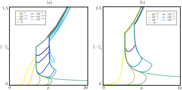
Figure 12: Solution branches for different values of $z_{1}(0)\equiv\eta$ when $\alpha=5$, $\varepsilon=1/144$ in system (4.5)–(4.6) (panel (a)), and when $\alpha=1$, $\varepsilon=1/144$ in system (6.14)–(6.15) (panel (b)). The panels show branches for $z_{1}(0)=\eta\neq 0$; these differ in the sign of $\eta$ (see legend) and are organized by an orbit-flip bifurcation at $\mu=\mu_{\ast}$ (see text). The origin of the additional branches revealed in this figure, including the second vertical segment at $\mu=\mu_{c+}$, is discussed in Appendix A.

It is important to mention that other scalings of our model system (1.1) are possible. Of these, the scaling

$$0<\varepsilon=U^{-2}\ll 1,\quad\alpha\to\varepsilon^{-1/2}\alpha,\quad x\to\varepsilon^{1/2}x,\quad t\to\varepsilon t,$$

leads to the spatial dynamical system

(6.14) $$z^{\prime}_{1} =-z_{2}+z_{1}-\frac{\alpha}{3}z_{1}^{3}$$

(6.15) $$z^{\prime}_{2} =\varepsilon(\mu z_{1}-z_{1}^{3}).$$

In this scaling it is easier to discuss canards (see Appendix A), but the bifurcation structure of systems (4.5)–(4.6) and (6.14)–(6.15) is very similar, as confirmed by the bifurcation diagrams in Figure 12. Indeed, the rescaling leading to Eqs. (6.14)–(6.15) demonstrates the robustness of the behavior we have described here with respect to changes in the physical parameters of the system.

The problem as formulated here contains two independent parameters, the forcing parameter $\mu$ responsible for the primary instability and the advection speed $U$. Similar situations arise in Rayleigh-Bénard convection with throughflow. This problem has been studied by a number of authors, both for transverse rolls [29] and longitudinal rolls [30]. However, in both these cases the pattern-forming instability is supercritical. This is also the case for Taylor vortices in a Taylor-Couette system with axial flow [3, 33]. Related work on binary fluid convection [4] studies a subcritical system but with periodic boundary conditions, thereby eliminating the possible influence of inlet perturbations. The effect of such perturbations is usually studied within a linearized theory [11] or via numerical simulations, either of model equations [11, 12, 8] or the full partial differential equations [24, 30]. However, in no case has the full bifurcation diagram been computed for nonzero inlet boundary conditions as done here.

In contrast, in shear flow instability, including plane Poiseuille (channel) flow and circular Poiseuille (pipe) flow, the shear flow is simultaneously responsible for the presence of finite amplitude instability of the laminar state and the advection of the resulting turbulent structures downstream [13, 19]. Such flows are therefore fundamentally different from the problem studied here, and indeed in carefully controlled pipe flow experiments the laminar state persists to large values of the Reynolds number ($Re\sim 60\,000$ [19]), the parameter that simultaneously quantifies both the shear rate and the advection velocity, despite the inevitable presence of inlet fluctuations. For comparison, finite amplitude perturbations trigger pipe flow turbulence at $Re\sim 2\,000$.

We mention that Eq. (1.1), in the form $A_{t}=A_{xx}-(U-\alpha|A|^{2})A_{x}+\mu A-|A|^{2}A$, may also be considered to be an amplitude equation for the complex amplitude $A(x,t)$ of a wavetrain of the form $A(x,t)\exp ikx$. The real subspace of this equation is invariant and identical to Eq. (1.1). The stationary solutions to this BVP constructed here therefore remain solutions of this higher-dimensional system; the zeros of $A(x)$ now correspond to phase defects – locations where the phase of the solution jumps by $\pi$, and it is possible that the breakup of a wavetrain into domains with different phase speeds observed in simulations of the complex Ginzburg-Landau equation with drift [22, 38] can be understood along these lines.

In summary, we expect that the ideas presented in this work may find application in different areas of fluid mechanics where a strongly subcritical instability interacts with an imposed flow.

Appendix A Phase plane analysis

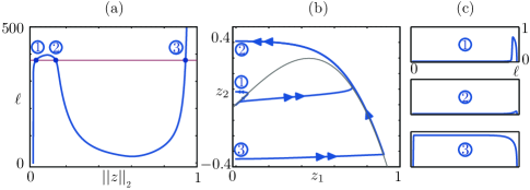
Figure 13: (a) Solution branch of Eqs. (4.5)–(4.6) obtained by varying $\ell$ for fixed $\mu=10$, $\alpha=5$ and $\eta=10^{-13}$ for comparison with Figure 5. Three solutions are found for $\ell=377$, shown in panels (b) and (c).

In this section, we refer to convective (absolute) instability states as type I (type II) solutions. As explained in Section 4.1, BVP (4.5)–(4.7) with $\eta=0$ has a pair of solutions for $\mu>\mu_{\ast}$, one of which disappears when its $L_{2}$ norm vanishes. This occurs, by definition, at $\mu=\mu_{\mathrm{g}}$. Since $\mu_{\mathrm{g}}\approx\mu_{\mathrm{a}}$ for large $\ell$ we conclude that these solutions are fundamentally a consequence of absolute instability of the trivial state $A=0$ that takes place at $\mu=\mu_{\mathrm{a}}$ and hence of type II. Both solutions start at $z_{2}(0)<0$ and follow the fast dynamics to the vicinity of the critical manifold $N$ above $P_{+}$, then drift along $N$ past $M_{+}$, and finally return to the $z_{2}$ axis with $z_{2}(\ell)>0$ (see Figure 5(b)). In the following we refer to solutions for which $z_{2}(0)\approx 0$ as type IIa, and to solutions for which the point $(0,z_{2}(0))$ is close to $W^{s}(P_{+})$ as type IIb (we assume $\ell$ is large). Note that no type II solutions are present for $\mu<\mu_{\ast}$. The above statements can be made rigorous in the setting of system  (6.14)–(6.15) and explain the transition between sectors 1 and 2 in Figure 4 and the role of the parameter value $\mu=\mu_{*}$.

We now consider BVP (4.5)–(4.7) with $\eta\neq 0$, which introduces a small but generic perturbation of the $\eta=0$ case that results in a new class of solutions (Figures 3 and 6). We think of the boundary condition $0<|\eta|\ll 1$ as reflecting the presence of small amplitude imperfections or “noise” at the inlet. This perturbation has a number of consequences. It results in the presence of a nontrivial type I state, and introduces a reconnection between this state and the type IIa branch very close to $\mu=\mu_{\mathrm{g}}$ via a fold bifurcation at $\mu=\mu_{\eta}$ (Figure 6(a)); the location of this fold is extremely sensitive to the value of $\eta$. Branch IIa then continues to larger amplitude and smaller $\mu$ towards the limit point bifurcation at $\mu_{\ast}$ (we ignore here the very weak dependence of $\mu_{\ast}$ on $\eta$) where it connects to the upper IIb branch. It follows that for the perturbed BVP, with $|\eta|$ very small, there is an interval $[\mu_{\ast},\mu_{\eta}]$ of $\mu$ values, with $\mu_{\eta}<\mu_{\mathrm{g}}$ ($\mu_{\eta}\to\mu_{g}$ as $\eta\to 0$), for which both solutions of type II remain (see Figures 5 and 12(a)). Since type I solutions are also present, it follows that for any fixed $\mu\in[\mu_{\ast},\mu_{\eta}]$ there are three different solutions to the perturbed BVP as illustrated in Figure 13 (as before, we take $\ell$ large). Moreover, for each $\eta>0$, no matter how small, there exists a solution of the perturbed BVP with $z_{2}(0)>0$ defined on the interval $\mu\in(0,\mu_{\eta})$. These type I solutions (Figure 6(c)) contain segments that follow $N^{r}$ but ultimately connect to an attracting fast fiber and so resemble the faux canards familiar from the ODE setting, a term used to refer to solutions that start on a repelling slow manifold and connect to an attracting slow manifold [28]. Other notable solutions in slow-fast ODEs are jump-on canards, which start along an attracting fast fiber and connect to a repelling slow manifold [16]. Type I solutions feature this behavior in reverse ’time’.

The phase plane plots show that, initially, when $\mu$ is small, these solutions return very quickly to the $z_{1}$ axis and their canard segments are very short. However, as $\mu$ increases so does the length of the canard segment. For $\mu$ close to $\mu_{\eta}$ the solution of type IIa also develops a canard segment and finally at $\mu=\mu_{\eta}$ the solutions of type I and type IIa merge in a limit point bifurcation at $\mu_{\eta}$. For $\mu>\mu_{\eta}$ there exists only one solution, corresponding to type IIb. Note that for $\mu\in(\mu_{\ast},\mu_{\eta})$ there exist three distinct solutions (see Figure 12(a) for the smallest values of $\eta$). The presence of the limit point $\mu_{\eta}$ is thus related to the transition from solutions analogous to canard cycles with no head to ones analogous to canard cycles with a head (see Figure 14 and [15]). For larger $\eta$ the limit point $\mu_{\eta}$ disappears and solutions of type I change by homotopy to solutions of type II.

Figure 14: (a) Detail of the type I solution branch with $\eta=-10^{-7}$ from Figure 12(a). (b) Portion of the phase plane showing the trajectories corresponding to the locations indicated in (a). Spatial profiles of the solutions of BVP (4.5)–(4.7) with $\eta<0$ corresponding to the trajectories shown in (b) are shown alongside. For the parameter values of Figure 12(a) $\mu_{\ast}\approx 6.84$ and $\mu_{c+}\approx 10.19$.

Case $\eta>0$: Figure 6(a) shows a detail of the branch corresponding to $\eta=10^{-10}$ in Figure 12(a). The numbers 1–11 refer to points along this branch and the corresponding phase portraits are shown in Figure 6(b). Note that in contrast to the canard explosions that occur in exponentially small intervals in two-dimensional systems [2], in the present case no canard explosion takes place and canard behavior occurs over an $O(1)$ interval of values of the parameter $\mu$. The absence of an explosive passage through the canard family is due to the nature of the BVP we consider: we fix $\ell$, $z_{1}(0)$ and $z_{1}(\ell)$. Solutions to this BVP compensate changes in $\mu$ by adjustments of $z_{2}(0)$, which controls the distance between $(z_{1}(0),z_{2}(0))$ and the repelling slow manifold. A nearby solution containing a canard segment adjusts the distance between $(z_{1}(0),z_{2}(0))$ and the repelling manifold, so that the passage time for the adjusted $\mu$ value is $\ell$: since the passage time along this manifold does not vary much with $\mu$, the updated solution has a canard segment as well. Usually canards are computed as solutions to a different BVP, where $z_{2}(0)$ is fixed and $\ell$ is a free parameter. In this case solutions have canard segments only for a small range of $\mu$, near the value defined by $(z_{1}(0),z_{2}(0))$ on a repelling slow manifold, and hence explosive behavior occurs.

Case $\eta<0$: We next consider the perturbed BVP with $\eta<0$. Associated solution branches are shown in Figure 12(a) and in close-up in Figure 14, which shows the corresponding solution profiles. Below we describe the solutions labeled $0,1,\ldots$ in Figure 14. Solution labeled 0 is very similar to a type IIb solution of the unperturbed BVP: it starts close to an unstable fiber of $N$, jumps to $N^{+}$, follows it to $M_{+}$ and returns to the $z_{2}$ axis along a fast fiber. As $\mu$ decreases towards $\mu_{\ast}$ and $P_{+}$ moves up along $N$, all solutions are of this type. This is very similar to the situation for $\eta>0$, since segments of these branches (for $\mu>\mu_{\ast}$) remain close to the corresponding solution branches IIa,b in the unperturbed BVP. The vertical segment between labels 1 and 2 corresponds to a passage near the orbit flip transition and along a segment of the branch of solutions of type IIb. The branch is similar to the branches of solutions for $\eta>0$ as it follows the unperturbed solution branch corresponding to solutions of type IIb for $\mu$ up to a certain value that increases as $\eta$ decreases. However, the relevant solutions with $\eta<0$ differ from the corresponding solutions with $\eta>0$ in that they leave the vicinity of the unperturbed branch ($z_{1}(0)=0$) in the opposite direction (see Figure 12(a)). After that, the solutions start developing a canard segment and the branch has a fold that corresponds to the maximal canard segment. The main difference from the branches with $\eta>0$ is that canard segments with $z_{1}(0)=-\eta$ follow $N^{r}$ to the left of the vertical axis; compare solutions 2 to 8 in Figure 14 with solutions 9 to 11 in Figure 6. Past the fold point, solutions with $\eta<0$ containing a canard segment make an excursion towards $N^{-}$ before jumping at $M_{-}$ and following $N^{+}$ towards $M_{+}$; see solutions 8 to 14 in Figure 14. For the range of $\mu$ values where this occurs, the saddle point $P_{+}$ lies below $M_{-}$. As $\mu$ approaches the value of $\mu_{c+}$, which corresponds to a connection from the maximal canard to $P_{+}$ (see Figures 14(b) and 15) the corresponding solutions, after jumping near $M_{-}$, come closer and closer to $P_{+}$, which incurs a large increase of the $L_{2}$ norm for a very small change in $\mu$ (of the order of $10^{-3}$). This argument explains the presence of the second vertical part of the branch seen in Figure 14(a) at $\mu=\mu_{c+}$. We mention that $\mu_{c+}$ is extremely close to the value $\mu=\mu_{h}$ at which there is, in the limit $\varepsilon\to 0$, a heteroclinic orbit connecting $P_{+}$ to $P_{-}$ via the turning points $M_{\pm}$. However, the latter solutions are of no relevance to any of the BVP considered in the present work.

Figure 15: (a) Trajectory 5 (thick gray-blue line), containing a canard segment, from Figure 14; also shown is a portion of the phase plane showing the repelling and attracting nullclines as well as stable and unstable manifolds of the three equilibria of the system present at this value of $\mu$. (b) Spatial profile of the corresponding solution to the perturbed BVP (4.5)–(4.7) with $\eta<0$.

We may think of the type I solutions as small amplitude solutions and type II solutions as large amplitude solutions. The former originate in convective instability that sets in at $\mu=0$ in the absence of boundaries while the latter arises from absolute instability. Both solutions exist when $P_{+}$ lies below the $z_{1}$ axis but as $\mu$ decreases and $P_{+}$ moves above the axis type II solutions are destroyed via a special solution that follows the strong unstable manifold of the origin to $P_{+}$ [9]. Solutions leaving $O$ along this manifold are characterized by very rapid increase in amplitude, followed by a lengthy interval at amplitude $z_{1}\approx\mathchoice{{\hbox{$\displaystyle\sqrt{\mu\,}$}\lower 0.4pt\hbox{\vrule height=4.30554pt,depth=-3.44446pt}}}{{\hbox{$\textstyle\sqrt{\mu\,}$}\lower 0.4pt\hbox{\vrule height=4.30554pt,depth=-3.44446pt}}}{{\hbox{$\scriptstyle\sqrt{\mu\,}$}\lower 0.4pt\hbox{\vrule height=3.01389pt,depth=-2.41113pt}}}{{\hbox{$\scriptscriptstyle\sqrt{\mu\,}$}\lower 0.4pt\hbox{\vrule height=2.15277pt,depth=-1.72223pt}}}$ before decaying back to $z_{1}=0$ at $x=\ell$. This condition determines the condition for an orbit flip; as already mentioned, in the limit $\varepsilon\rightarrow 0$, this condition is equivalent to the passage of $P_{+}$ through the $z_{1}$ axis, i.e., to $\mu=(3/\alpha)\varepsilon^{-1/2}$. When $\alpha=O(1)$ the location of this point moves to large values of $\mu$; however, in system (6.14)–(6.15), this transition occurs at a finite value of $\mu$, $\mu=3/\beta$. In fact, in the definition of type I/type II solutions we can replace the $z_{1}$ axis by (one of the branches of) the strong unstable manifold $W^{\rm uu}(O)$; for $\varepsilon\approx 0$ these two sets are very close to one another since the slope of the eigenvector associated with the strong eigenvalue of the origin converges to $0$ as $\varepsilon\to 0$. Specifically, a solution is of type I if $(\eta,z_{2}(0))$ is above $W^{\rm uu}(0)$ and of type II if $(\eta,z_{2}(0))$ is below $W^{\rm uu}(O)$. A solution of type I or II which passes near $N^{+}$ exists only if $(\eta,z_{2}(0))$ is above $W^{s}(P_{+})$. It follows that solutions of type I can be found as long as $P_{+}$ is below $M_{+}$, while solutions of type II exist only if $\mu>\mu_{\ast}$, i.e., $W^{s}(P_{+})$ is below $W^{\rm uu}(O)$. This is consistent with the discussion in the preceding paragraphs.

In fact there is another class of solutions to the perturbed BVP, corresponding, in phase space, to one or more full turns around the origin before returning to the $z_{1}$ axis at $x=\ell$. These solutions follow the heteroclinic cycle mentioned above, and we can understand their behavior using the same phase plane analysis. We focus on the branch in the central panel of Figure 16. The properties of the solutions on this branch can be classified by their behavior near the origin and near the saddle points $P_{\pm}$. For example, the solution labeled 7 is at a fold point of the branch. Like solution 5 from Figure 15, it contains a maximal canard segment; the explanation of that fold point is similar to that provided earlier. Solutions 5 and 6 in Figure 16 occur after and before the transition through the maximal canard, respectively. Solutions 1 and 2 are located at local maxima on the branch and the associated $\mu$ values are both very close to the (right) vertical segment on the branch shown in Figure 14(a); as in the similar cases discussed earlier, these solutions come close to either of the two saddle points, explaining the sharp increase in their $L_{2}$ norm. Lastly, solution 3 is close to a type II solution, and solution 4 is very similar to such a solution but with $z_{2}(0)$ positive. Solutions with more turns are also possible and behave analogously.

Figure 16: Branch (central panel) corresponding to solutions that make a full turn around $N$ before connecting back to $z_{1}=0$. The central panel shows a zoom of the rightmost branch from Figure 12(a) corresponding to $\eta=-10^{-10}$. Side panels show different solution profiles in space and in the phase plane at different locations along this branch as indicated by the inscribed integers.

Finally, since the transition from the branch with $\eta=0$ to the branches with $\eta\neq 0$ can be seen as a broken pitchfork bifurcation, we expect to find disconnected solution branches for $\mu>\mu_{\mathrm{g}}$ and $\eta\neq 0$. These are indeed present, as shown in Figure 17 for $\eta=10^{-7}$ and $\eta=10^{-5}$. The solution profiles on these branches correspond to orbit segments that make several turns along $N$ before connecting back to $z_{1}=0$, and these lie, in the limit $\varepsilon\to 0$, on additional solution branches of the unperturbed BVP. In fact, for $\ell$ sufficiently large, there will be many such solutions to the BVP considered by Chomaz & Couairon, depending on the number of turns they make along $N$ before connecting back to $z_{1}=0$. When the inlet boundary condition becomes $z_{1}(0)=\eta\neq 0$ with $\eta$ small (positive or negative), one finds solution branches that follow the unperturbed ($\eta=0$) branches corresponding to a given number of turns; such branches may also connect two such unperturbed branches, as shown in Figure 17. Note that all the branches that exist in the range $\mu>\mu_{\mathrm{g}}$ have regular limit points without vertical segments, in contrast to the branches passing through $\mu=\mu_{\ast}$ and $\mu=\mu_{c+}$. This is because for $\mu>\mu_{\mathrm{g}}$ the unstable equilibrium point at the origin acquires complex eigenvalues (thereby preventing orbit flips) so that the long-term dynamics of the ODE system (4.5)–(4.6) takes the form of an attracting limit cycle surrounding the origin (thereby preventing any connection between the origin and the saddle points $P_{\pm}$). Stability calculations show that these additional solutions are all unstable (in time).

Figure 17: Solution branches for $\mu>\mu_{\mathrm{g}}\approx 36.030$, for both $\eta=0$ and $\eta>0$ (see legend). The solutions resemble those shown in Figure 16, but with more than one full turn along $N$. Unlike the type I and II branches described earlier these branches do not exhibit any vertical segments. This is a consequence of the fact that for $\mu>\mu_{\mathrm{g}}$ the origin $(0,0)$ has complex (spatial) eigenvalues.

Appendix B Appendix: Numerical methods

This appendix summarizes the numerical technique used to obtain the results reported in this paper. We discretize the PDE (3.2) using a grid of evenly spaced points $x=\{x_{i}\}_{i=1}^{n+1}$, with $x_{i}=i\ell/n$, and construct the approximation vectors $A(t)=\{A_{i}(t)\}$, where $A_{i}(t)\approx A(x_{i},t)$. We employ the method of lines to obtain a large set of nonlinear ODEs

(2.16) $$A_{1} =\eta,$$

$$\dot{A}_{i} =\varepsilon\mu A_{i}-\mathchoice{{\hbox{$\displaystyle\sqrt{\varepsilon\,}$}\lower 0.4pt\hbox{\vrule height=4.30554pt,depth=-3.44446pt}}}{{\hbox{$\textstyle\sqrt{\varepsilon\,}$}\lower 0.4pt\hbox{\vrule height=4.30554pt,depth=-3.44446pt}}}{{\hbox{$\scriptstyle\sqrt{\varepsilon\,}$}\lower 0.4pt\hbox{\vrule height=3.01389pt,depth=-2.41113pt}}}{{\hbox{$\scriptscriptstyle\sqrt{\varepsilon\,}$}\lower 0.4pt\hbox{\vrule height=2.15277pt,depth=-1.72223pt}}}A^{3}_{i}+\sum_{j=1}^{n+1}\Big{[}\lnot{\dagger}(D^{2}_{x})_{ij}-(1-\alpha A^{2}_{i})(D_{x})_{ij}\Big{]}A_{j}\quad i=2,\ldots,n,$$

$$A_{n+1} =0,$$

where $D_{x}$ and $D^{2}_{x}$ are $(n-1)\times(n+1)$ finite-difference differentiation matrices for the operators $\partial_{x}$ and $\partial_{xx}$, respectively. In all PDE computations we use $n=4000$ gridpoints. Time stepping is performed using MATLAB’s ode23s with default parameters and explicitly formed Jacobian. For the stochastic time stepping we use a standard Euler-Maruyama time-stepping scheme [27] with $s=10^{-3}$. Steady states are computed using MATLAB’s fsolve with default parameter values and continued in parameter space using the routines developed in [32]. Stability of a steady state $A_{*}=\{A_{*}(x_{i})\}$ is studied by computing the first $40$ eigenvalues of the problem $M\psi=J(A_{*})\psi$ with the smallest absolute value, where

$$M=\mathrm{diag}(0,1,\ldots,1,0)\in\mathbb{R}^{(n+1)\times(n+1)},$$

$$J=\begin{bmatrix}e_{1}\\ D^{2}_{x}-\mathrm{diag}(1-\alpha A^{2}_{*})D_{x}+\mathrm{diag}(2\alpha A_{*}D_{x}A_{*}+\varepsilon\mu-3\mathchoice{{\hbox{$\displaystyle\sqrt{\varepsilon\,}$}\lower 0.4pt\hbox{\vrule height=4.30554pt,depth=-3.44446pt}}}{{\hbox{$\textstyle\sqrt{\varepsilon\,}$}\lower 0.4pt\hbox{\vrule height=4.30554pt,depth=-3.44446pt}}}{{\hbox{$\scriptstyle\sqrt{\varepsilon\,}$}\lower 0.4pt\hbox{\vrule height=3.01389pt,depth=-2.41113pt}}}{{\hbox{$\scriptscriptstyle\sqrt{\varepsilon\,}$}\lower 0.4pt\hbox{\vrule height=2.15277pt,depth=-1.72223pt}}}A^{2}_{*})\\ e_{n+1}\end{bmatrix}\in\mathbb{R}^{(n+1)\times(n+1)}$$

and the $\{e_{i}\}$ are row vectors forming the canonical basis of $\mathbb{R}^{n+1}$.

References

- [1] D. Avitabile, M. Desroches, and E. Knobloch, Spatiotemporal canards in neural field equations, Physical Review E 95 (2017), pp. 042205.
- [2] E. Benoît, J.-L. Callot, F. Diener and M. Diener, Chasse au canard, Collectanea Matematica 32 (1981), pp. 37–119.
- [3] P. Büchel, M. Lücke, D. Roth and R. Schmitz, Pattern selection in the absolutely unstable regime as a nonlinear eigenvalue problem: Taylor vortices in axial flow, Physical Review E 53 (1996), pp. 4764–4777.
- [4] P. Büchel and M. Lücke, Influence of through flow on binary convection, Physical Review E,61 (2000), pp. 3793–3810.
- [5] L. Buřič, A. Klíč and L. Purmová, Canard solutions and travelling waves in the spruce budworm population model, Applied Mathematics and Computation 183 (2006), pp. 1039–1051.
- [6] P. Carter, E. Knobloch and M. Wechselberger, Transonic canards and stellar wind, Nonlinearity 30 (2017), pp. 1006–1033.
- [7] K. W. Chang and F. A. Howes, Nonlinear Singular Perturbation Phenomena: Theory and Applications. Springer Science & Business Media, 1984.
- [8] P. Colet, D. Walgraef and M. San Miguel, Convective and absolute instabilities in the subcritical Ginzburg-Landau equation, The European Physical Journal B 11 (1999), pp. 517–524.
- [9] A. Couairon and J.-M. Chomaz, Absolute and convective instabilities, front velocities and global modes in nonlinear systems, Physica D 108 (1997), pp. 236–276.
- [10] J.-M. Chomaz and A. Couairon, Against the wind, Physics of Fluids 11 (1999), pp. 2977–2983.
- [11] R. J. Deissler, Spatially growing waves, intermittency, and convective chaos in an open-flow system, Physica D 25 (1987), pp. 233–260.
- [12] R. J. Deissler, Turbulent bursts, spots and slugs in a generalized Ginzburg-Landau equation, Physics Letters A 120 (1987), pp. 334–340.
- [13] R. J. Deissler, The convective nature of instability in plane Poiseuille flow, Physics of Fluids 30 (1987), pp. 2303–2305.
- [14] E. M. De Jager and J. F. Furu, The Theory of Singular Perturbations, Elsevier (1996).
- [15] P. De Maesschalck and M. Desroches, Numerical continuation techniques for planar slow-fast systems, SIAM Journal on Applied Dynamical Systems 12 (2013), pp. 1159–1180.
- [16] P. De Maesschalck, F. Dumortier and R. Roussarie, Cyclicity of common slow-fast cycles, Indagationes Mathematicae 22 (2011), pp. 165–206.
- [17] P. De Maesschalck, N. Popović and T. J. Kaper, Canards and bifurcation delays of spatially homogeneous and inhomogeneous types in reaction-diffusion equations, Advances in Differential Equations 14 (2009), pp. 943–962.
- [18] M. Desroches, J. Guckenheimer, B. Krauskopf, C. Kuehn, H. M. Osinga and M. Wechselberger, Mixed-mode oscillations with multiple time scales, SIAM Review 54 (2012), pp. 211–288.
- [19] B. Eckhardt, T. M. Schneider, B. Hof and J. Westerweel, Turbulence transition in pipe flow, Annual Review of Fluid Mechanics 39 (2007), pp. 447–468.
- [20] N. Fenichel, Geometric singular perturbation theory, Journal of Differential Equations 31 (1979), pp. 53–98.
- [21] P. Gandhi, C. Beaume and E. Knobloch, Time-periodic forcing of spatially localized structures, Nonlinear Dynamics: Materials, Theory and Experiments (M. Tlidi and M. G. Clerc, eds), Springer Proceedings in Physics 173 (2016), pp. 303–316.
- [22] J. B. Gonpe Tafo, L. Nana and T. C. Kofane, Nonlinear structures of traveling waves in the cubic-quintic complex Ginzburg-Landau equation on a finite domain, Physica Scripta 87 (2013), 065001.
- [23] J. Härterich, Viscous profiles of traveling waves in scalar balance laws: the canard case, Methods and Applications of Analysis 10 (2003), pp. 97–118.
- [24] D. Jung, M. Lücke and A. Szprynger, Influence of inlet and bulk noise on Rayleigh-Bénard convection with lateral flow, Physical Review E, 63 (2001), 056301.
- [25] W. L. Kath and J. D. Murray, Analysis of a model biological switch, SIAM Journal on Applied Mathematics 45 (1985), pp. 943–955.
- [26] M. Krupa and P. Szmolyan, Relaxation oscillation and canard explosion, Journal of Differential Equations 174 (2001), pp. 312–368.
- [27] G. Lord, C. E. Powell and T. Shardlow, An Introduction to Computational Stochastic PDEs, Cambridge University Press (2014).
- [28] J. Mitry and M. Wechselberger, Folded saddles & faux canards, SIAM Journal on Applied Dynamical Systems 16 (2017), pp. 546–596.
- [29] H. W. Müller, M. Lücke and M. Kamps, Transversal convection patterns in horizontal shear flow, Physical Review A 45 (1992), pp. 3714–3726.
- [30] X. Nicolas, N. Zoueidi and S. Xin, Influence of a white noise at channel inlet on the parallel and wavy convective instabilities of Poiseuille-Rayleigh-Bénard flows, Physics of Fluids 24 (2012), 084101.
- [31] R. E. O’Malley, Jr., Singularly perturbed linear two-point boundary value problems, SIAM Review 50 (2008), pp. 459–482.
- [32] J. Rankin, D. Avitabile, J. Baladron, G. Faye and D. J. B. Lloyd, Continuation of localised coherent structures in nonlocal neural field equations, SIAM Journal on Scientific Computing 36 (2014), pp. B70–B93.
- [33] A. Recktenwald, M. Lücke and H. W. Müller, Taylor vortex formation in axial through-flow: Linear and weakly nonlinear analysis, Physical Review E 48 (1993), pp. 4444–4454.
- [34] S. C. Reddy and L. N. Trefethen, Pseudospectra of the convection-diffusion operator, SIAM Journal on Applied Mathematics 54 (1994), pp. 1634–1649.
- [35] G. N. Gorelov and V. A. Sobolev, Mathematical modeling of critical phenomena in thermal explosion theory, Combustion and Flame 87 (1991), pp. 203-210.
- [36] G. N. Gorelov and V. A. Sobolev, Duck-trajectories in a thermal explosion problem, Applied Mathematics Letters 5 (1992), pp. 3–6.
- [37] K. R. Schneider, E. A. Shchepakina and V. A. Sobolev, New type of travelling wave solutions, Mathematical Methods in the Applied Sciences 26 (2003), pp. 1349–1361.
- [38] S. M. Tobias, M. R. E. Proctor and E. Knobloch, Convective and absolute instabilities of fluid flows in finite geometry, Physica D 113 (1998), pp. 43–72.
- [39] L. N. Trefethen and D. Bau III, Numerical Linear Algebra, SIAM, Philadelphia (1997).
- [40] L. S. Tuckerman, T. Kreilos, H. Schrobsdorff, T. M. Schneider and J. F. Gibson, Turbulent-laminar patterns in plane Poiseuille flow, Physics of Fluids 26 (2014), 114103.
- [41] M. Wechselberger and G. J. Pettet, Folds, canards and shocks in advection-reaction-diffusion models, Nonlinearity 23 (2010), pp. 1949–1969.