Present address: ]Centre for Theoretical Atomic, Molecular and Optical Physics, School of Mathematics and Physics, Queen’s University Belfast, Belfast BT7 1NN, Northern Ireland, United Kingdom
The approach to chaos in ultracold atomic and molecular physics:
statistics of near-threshold bound states for Li+CaH and Li+CaF
Abstract
We calculate near-threshold bound states and Feshbach resonance positions for atom + rigid-rotor models of the highly anisotropic systems Li+CaH and Li+CaF. We perform statistical analysis on the resonance positions to compare with the predictions of random matrix theory. For Li+CaH with total angular momentum we find fully chaotic behavior in both the nearest-neighbor spacing distribution and the level number variance. However, for we find different behavior due to the presence of a nearly conserved quantum number. Li+CaF () also shows apparently reduced levels of chaotic behavior despite its stronger effective coupling. We suggest this may indicate the development of another good quantum number relating to a bending motion of the complex. However, continuously varying the rotational constant over a wide range shows unexpected structure in the degree of chaotic behavior, including a dramatic reduction around the rotational constant of CaF. This demonstrates the complexity of the relationship between coupling and chaotic behavior.
I Introduction
There is currently great interest in the behavior of atoms and molecules at ultracold temperatures. Work in this field focussed initially on simple systems, which are amenable to detailed control by tuning with applied fields Chin et al. (2010). Particular success has been achieved with ultracold collisions and high-lying bound states of pairs of alkali-metal atoms, where a combination of experiment and theory has produced a detailed understanding for a variety of different systems Takekoshi et al. (2012); Berninger et al. (2013); Julienne and Hutson (2014). This understanding has been used to study solitons in Bose-Einstein condensates Frantzeskakis (2010), diatomic molecule formation Köhler et al. (2006), Efimov states Kraemer et al. (2006); Huang et al. (2014) and many other phenomena. However, attention is now turning to increasingly complex systems, such as collisions of high-spin atoms Lu et al. (2011); Pasquiou et al. (2012); Aikawa et al. (2012); Baumann et al. (2014); Maier et al. (2015a); Frisch et al. (2015) and ground-state molecules Ni et al. (2008); Ospelkaus et al. (2010); Parazzoli et al. (2011); Takekoshi et al. (2014); Molony et al. (2014). The theory needed for a full description of these systems is often prohibitively difficult; for example, two erbium atoms interact on 91 potential curves Frisch et al. (2014), so that it is unrealistic to fit precise potentials to experimental results in the manner that has been so successful for alkali dimers Takekoshi et al. (2012); Berninger et al. (2013); Julienne and Hutson (2014). In these circumstances, it is possible that the dynamics are stochastic, with levels described by random matrix theory Mehta (1991); Guhr et al. (1998). These ideas were first developed in the theory of compound nuclei Wigner (1955); Dyson (1962), and underlie current thinking about the nature of quantum chaos.
A qualitative understanding of the dynamics of these highly complex systems is important for both theorists and experimentalists. For a simple system, theory can in principle give a complete description, but for a fully chaotic system specific predictions are likely to be impossible. For example, it is unlikely to be possible to map out the near-threshold bound states navigated by Feshbach molecules except empirically Frisch et al. (2015). If a collision is chaotic in nature, the collision complex will ergodically explore the entire phase-space and the two collision partners may be trapped together for a long time. In ultracold collisions, this may be long enough for a third body to collide with the complex, which is likely to lead to the loss of all the particles involved from the trap Mayle et al. (2012).
Random matrix theory (RMT) was first applied to ultracold collisions by Mayle et al., initially for atom+diatom collisions Mayle et al. (2012) and later for diatom+diatom collisions Mayle et al. (2013). The first experimental demonstration of these ideas was provided by atom+atom collisions for Er+Er Frisch et al. (2014) and later Dy+Dy Maier et al. (2015b). Several theoretical models have also been analyzed in terms of RMT Jachymski and Julienne (2015); Frisch et al. (2014); Maier et al. (2015b). Within RMT the archetypal model of quantum chaos is a matrix ensemble known as the Gaussian Orthogonal Ensemble (GOE) Dyson (1962); Mehta (1991) and the usual way to assess whether or not chaos is present in a level sequence is to compare various statistics to the expectations from the GOE. In particular, the Bohigas-Giannoni-Schmit conjecture Bohigas et al. (1984) states that quantum systems whose classical analogues are chaotic will show the same level fluctuations as the GOE.
There are many statistics available to analyze level sequences (see for example chapter 16 of Mehta’s book Mehta (1991)) but work on ultracold collisions so far has focused on two of the simplest quantities: the distribution of nearest-neighbor spacings (NNS) and the level number variance. In ultracold collisions, the levels (or resonances) concerned are typically observed as a function of magnetic field rather than energy. Erbium and dysprosium have been found to have NNS distributions and number variances that are intermediate between those expected for chaotic and non-chaotic systems Frisch et al. (2014); Maier et al. (2015b). A re-analysis of the erbium results Mur-Petit and Molina (2015) showed that the deviations from chaotic predictions might arise because some narrow resonances are not observed in the experiment. A comparable degree of chaos has recently been found in coupled-channel calculations on the remarkably simple system Yb(1S)+Yb(3P) Green et al. (2016). However, similar calculations on Li+Er found statistics consistent with a random but non-chaotic level distribution González-Martínez and Żuchowski (2015).
Atom+diatom systems provide excellent prototype systems to investigate chaotic behavior. If vibrational excitation and electron spins are neglected, the systems have two internal degrees of freedom; this is the minimum for classical chaos and probably also for a quantum system to follow the predictions of RMT Bohigas et al. (1984). There are well-developed formalisms for treating collisions Bernstein (1979) and near-threshold bound states Hutson (1991, 1994) in atom+diatom systems, and readily available programs that efficiently perform the necessary calculations Hutson and Green (1994); Hutson (1993). There are many atom+diatom systems that are of interest at low temperatures, including Rb+KRb Ospelkaus et al. (2010), N+NH Hummon et al. (2011) and Li+CaH Lu et al. (2014).
The purpose of the present paper is to investigate quantum chaos in atom+diatom collisions. We investigate the statistics of levels at and near threshold for atom + rigid-rotor models of the highly anisotropic systems Li+CaH and Li+CaF, and compare them with the predictions of RMT. For simplicity, we neglect electron and nuclear spins. For Li+CaH with zero total angular momentum we find excellent agreement with RMT. However for higher angular momentum we find quite different behavior which we attribute to the presence of a nearly conserved quantum number. Li+CaF has a larger ratio of anisotropy to rotational constant than Li+CaH, and in this sense it is more strongly coupled, but we actually find it is less strongly chaotic, even for zero angular momentum. This shows that increasing coupling does not always make a system more chaotic and may, in some circumstances, return order to the system. We analyze statistics as a function of a continuously varying rotational constant, interpolating between CaH and CaF and beyond, and find complex behavior with apparently fluctuating levels of chaoticity.
II Potential energy surface
The interaction between Li(2S) and CaH/CaF() gives rise to singlet and triplet electronic states of 1A′ and 3A′ symmetries. For sympathetic cooling in an external magnetic field, Li and CaH/CaF would be prepared in magnetically trappable spin-stretched states, in which all the quantum numbers for the projections of angular momentum onto the magnetic field direction have their maximum values. Such collisions occur primarily on the potential energy surface for the 3A′ state, so we use this surface in the present paper.
For Li+CaH, we use the ab initio 3A′ interaction potential calculated by Tscherbul et al. Tscherbul et al. (2011). For Li+CaF, we carried out supermolecular coupled-cluster calculations of the 3A′ surface using a spin-restricted open-shell version of the coupled-cluster method with single, double and non-iterative triple excitations [RCCSD(T)], which is implemented in the MOLPRO package Werner et al. (2015). We used the aug-cc-pVTZ basis sets for each atom Dunning (1989); Kendall et al. (1992); Koput and Peterson (2002). Mid-bond functions (spdfg) were added at the midpoint between Li and CaF. The counterpoise correction of Boys and Bernardi Boys and Bernardi (1970) was used to compensate for basis set superposition error. In all our calculations the CaF bond length was fixed at the experimentally determined equilibrium value for the free diatom, 1.9516 Å Kaledin et al. (1999).
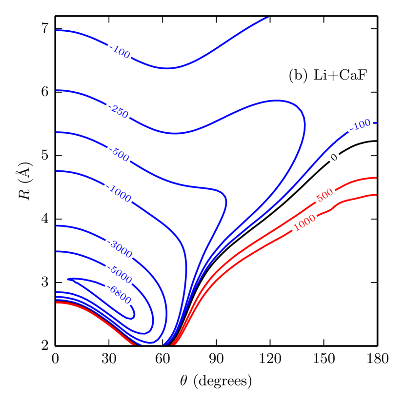
The resulting 3A′ potential energy surfaces are shown in Fig. 1, and it may be seen that they are strongly anisotropic, with a deep well (7063 cm-1 for CaH and 7258 cm-1 for CaF) at slightly bent Li--Ca geometries. The overall behavior of the two surfaces is similar, though the Li+CaF interaction is slightly stronger and more anisotropic.
III Bound-state calculations and statistics
When considering whether a system is chaotic, statistical analysis would usually be performed on a series of levels in energy with the Hamiltonian defining the system fixed. However, the underlying Random Matrix Theory concerns distributions taken over an ensemble of different Hamiltonians. The assumption that the distributions over energy (for a single Hamiltonian) are the same as those over Hamiltonians is known as spectral ergodicity Brody et al. (1981); this is a property of RMT but not necessarily of real systems. In recent ultracold collision studies Jachymski and Julienne (2015); Frisch et al. (2014); Maier et al. (2015b), statistical analysis was performed on a series of zero-energy resonance positions as magnetic field was varied. Such experiments sample many different Hamiltonians - albeit in a much more limited and structured way than RMT - and so may provide a more authentic comparison with RMT than an energy spectrum would, even if it was available. In place of the spectral ergodicity hypothesis, we now need only to assume that different Hamiltonians are sampled in a representative way.
Performing calculations on Li+CaH and Li+CaF in magnetic fields is a difficult and computationally expensive task, which is beyond the scope of this paper but will be investigated in the future. Instead, we vary the potential by an overall scaling factor Cvitaš et al. (2007); Wallis and Hutson (2009); Wallis et al. (2011), which also varies the Hamiltonian but without the theoretical complexities or computational expense associated with magnetic fields 111Note that even should not be interpreted as the true potential because there are significant uncertainties in the calculated potentials.. In this respect may be considered a “poor man’s magnetic field”. If a system shows signs of chaos with respect to , it is reasonable to label it chaotic (under the approximations made for the dynamics).
The theory of atom-diatom interactions is well established Bernstein (1979); Hutson (1991) and will not be repeated here. In the present work, we carry out close-coupling calculations in which the diatomic molecule is treated as a rigid rotor and its rotation is coupled to the end-over-end rotation of the collision complex to give the total angular momentum . We use coupled-channel propagation methods Hutson (1994) to locate bound states at threshold. We have modified the program FIELD Hutson (2011) to locate bound states as a function of rather than electric or magnetic field. We use the hybrid log-derivative propagator of Alexander and Manolopoulos Alexander and Manolopoulos (1987). Since the diatom rotational constants, , are very small ( cm-1 Tscherbul et al. (2011) and cm-1 Mizushima (1975)), we need very large basis sets of diatom rotational functions for convergence. Unless otherwise stated, we use basis functions with rotational quantum numbers up to and 120 for CaH and CaF, respectively.
The real systems include diatom vibrations and electron and nuclear spins. The harmonic frequencies for CaH and CaF are 1298 and 589 cm-1, respectively. Since the well depth is significantly larger than this, there will be states from channels involving diatom vibrational excitation in the region around threshold, although they may be sparse in energy. These are neglected in our calculations. There will also be considerable extra density of levels due to the spin multiplicities, although it is not clear whether the spins will be fully involved in any chaotic dynamics or if they will be spectators. The present results are therefore for model systems, based on the real systems but not taking account of their full complexity.
The Gaussian Orthogonal Ensemble (GOE) is the standard RMT model for chaos in systems with time-reversal-invariant Hamiltonians. It is a set of real symmetric matrices, with diagonal and off-diagonal elements described by probability distributions
| (1) | ||||
| (2) |
respectively, where and are normalization constants. The GOE has off-diagonal elements that are on the order of the spread of the diagonal elements and so for large are much larger than the average separation of diagonal elements. In the context of near-threshold bound states or low-energy collisions, this can occur when the anisotropic terms in the interaction are comparable in magnitude to the depth of the isotropic potential, which determines the spread of diagonal elements. The highly anisotropic potentials of Li+CaH and Li+CaF would seem to fulfil this: the majority of the potential well is contained in the anisotropic terms of many thousands of cm-1, which are significantly larger than the depth of the isotropic potential; the latter is only 1260 cm-1 for Li+CaH. In contrast, the Er+Er and Dy+Dy potentials used in Ref. Maier et al. (2015b) have anisotropies around 10% of their well depths 222The anisotropy considered in Ref. Maier et al. (2015b) is based entirely on dispersion effects Petrov et al. (2012). The spread of dispersion coefficients for different potential curves of Er-Er is 10% of their mean value, and that for Dy-Dy is 9% of their mean value.. In this way it is perhaps not surprising that there are deviations from GOE predictions for Er+Er and Dy+Dy, whereas we might at first sight expect better agreement for Li+CaH and Li+CaF.
For the statistical analysis of the levels we follow the methods of Mehta Mehta (1991) and Guhr et al. Guhr et al. (1998). We denote our series of calculated level positions as for 333We observe only a fraction of the total number of levels in the system, so .. First we ‘unfold’ the level positions to remove any systematic variation in the density and to set the levels on a dimensionless scale with unit mean spacing. To do this we construct the cumulative spectral function, also known as the staircase function,
| (3) |
where is the Heaviside step function. We then fit a smooth function, , to (in this paper, fitting with a quadratic is sufficient as the original staircase is already very nearly linear in ). The unfolded positions are then given as . The nearest-neighbor spacings (NNS) are given by for .
The NNS distribution is one of the main quantities of interest in statistical analysis. In particular, for the GOE the NNS distribution is very well approximated by the Wigner surmise Mehta (1991),
| (4) |
more commonly known as the Wigner-Dyson distribution, whereas for a random (uncorrelated) level sequence the NNS distribution is expected to follow a Poisson distribution,
| (5) |
Histograms of the NNS distribution provide a simple visual impression of the statistics. The Wigner-Dyson distribution exhibits strong level repulsion, dropping to zero at zero spacing, whereas the Poisson distribution peaks at zero spacing. The Wigner-Dyson distribution also falls to zero faster at large spacing than the Poisson distribution.
Real systems do not exactly follow either or . There are various formulas for interpolating between the two Berry and Robnik (1984); Izrailev (1988). The most commonly used of these, despite its lack of rigorous foundation, is the Brody distribution Brody (1973),
| (6) |
where
| (7) |
and is known as the Brody parameter. This is the NNS distribution that has been used in recent publications in ultracold physics and is the one that we use in this paper. We obtain a value of for a set of spacings by maximum likelihood estimation Barlow (1989). We maximise the likelihood function,
| (8) |
to find . Its uncertainty is
| (9) |
The fitted value for the Brody parameter quantifies the visual information seen in NNS histograms: Poisson statistics yield and chaotic statistics yield . If the pattern of energy levels is in fact regular, the NNS distribution is typically more strongly peaked than a Wigner-Dyson distribution Berry and Tabor (1977), and so the fitted Brody parameter may be greater than unity. We do find some fitted values , but they are consistent with within statistical uncertainties.
The NNS distribution by nature captures information only about short-range correlations but chaos is predicted to have effects over long ranges as well Mehta (1991); Guhr et al. (1998). Therefore we also consider the level number variance
| (10) |
where counts the number of levels in the interval and the average is taken over the starting values . This characterizes the spread in the numbers of levels in intervals of length and probes long-range correlations. It rises logarithmically for the GOE, rises linearly for Poisson statistics, and oscillates around a constant value for a regular system. While there have been some attempts to interpolate between Poissonian and GOE behaviors of the number variance, there is no direct analogue to the Brody distribution so we restrict ourselves to qualitative statements about the transition between the two limiting behaviors.
IV Results
IV.1 Li+CaH
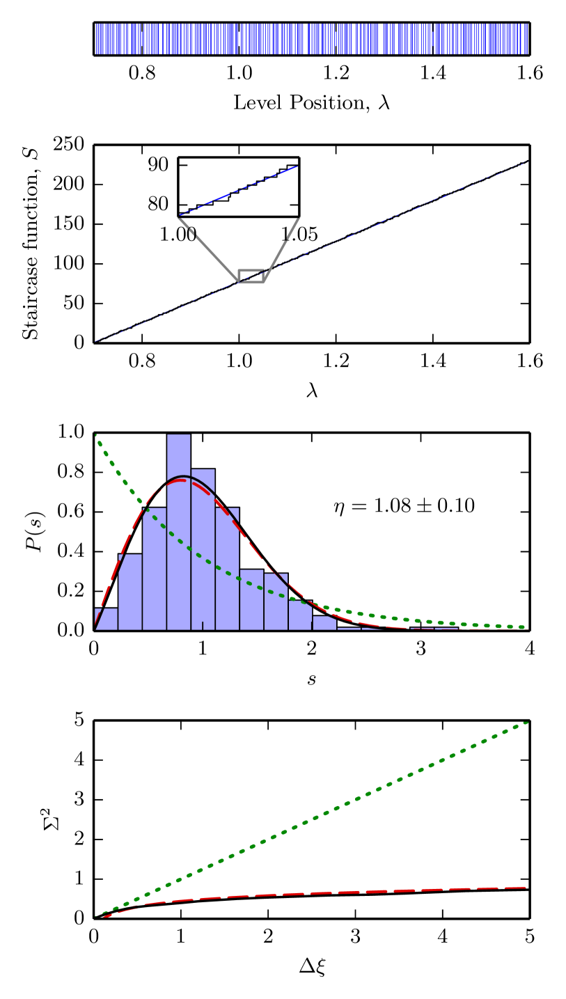
We begin by analyzing Li+CaH for total angular momentum and . Figure 2 shows the calculated level positions for , the staircase function, a histogram of the NNS distribution, and the level number variance. This serves as an example of the statistical preparation and fitting described in section III; all further sequences were analyzed in the same way. The NNS distribution clearly shows the key features of a Wigner-Dyson distribution: linear repulsion at small spacing and a tail that dies off rapidly. The fitted Brody parameter, , is consistent with GOE predictions, and the level number variance also follows the GOE prediction almost exactly. This Brody parameter may be compared with values in the region 0.5 to 0.7 found for Er+Er and Dy+Dy Maier et al. (2015b). Our recent work on Yb+Yb∗ Green et al. (2016) also found Brody parameters around 0.7 at high magnetic field, except in cases with relatively low numbers of levels. The rigid-rotor model of Li+CaH thus shows the clearest evidence yet found of chaotic behavior in ultracold collisions.
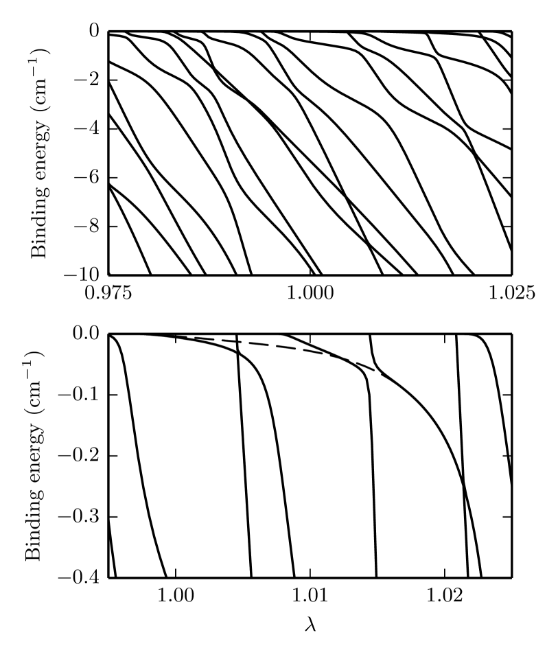
Figure 3 shows near-threshold bound states for for a small range of . The top panel shows bound states to a depth of 10 cm-1, where the levels interact and undergo avoided crossings with a wide variety of strengths. The lower panel is an expanded view showing a state with a long tail curving towards threshold. This state is crossed by several steeper states with avoided crossings of varying widths, including a crossing around that appears quite broad on this scale. Bound states with these features have been observed experimentally in Dy+Dy Maier et al. (2015a), although in our case the state is much more deeply bound (by a factor of about 100 in the natural units defined by the asymptotic van der Waals interaction relevant to such states Chin et al. (2010)). It is not a ‘halo’ state because its wave function is mostly inside the outer classical turning point Köhler et al. (2006), but its presence in Li+CaH demonstrates that states with clear threshold behavior can persist across several avoided crossings even in a system with statistics close to the Wigner-Dyson limit.
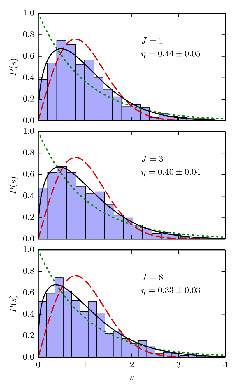
Next we consider higher values of , which correspond to higher partial waves at the lowest rotational threshold. Figure 4 shows histograms of NNS for =1, 3 and 8. These notably do not show the linear level repulsion at small spacings expected for complete chaos. Instead there appears to be a finite probability of zero spacing. The corresponding Brody parameters are in the region of 0.4. Although at first sight this suggests a substantially reduced degree of chaos compared to , such a distribution can also occur for two overlapping but non-interacting chaotic spectra Berry and Robnik (1984); Rosenzweig and Porter (1960). This suggests that there is some form of symmetry or good quantum number present in the system. However, we have already taken account of all rigorous symmetries, so the quantity concerned must be only approximately conserved. On a finer scale, the NNS distribution does indeed show some limited level repulsion.
The nearly conserved quantum number can be understood in the body-fixed reference frame, rather than the space-fixed frame that we use in the coupled-channel calculations. It is the projection of the total angular momentum (or equivalently the diatom rotation ) onto the intermolecular axis, which is well known in studies of atom-diatom Van der Waals complexes Hutson (1991) and is given the symbol . It can take values from to in integer steps. Blocks of the Hamiltonian with different are coupled only by Coriolis terms in the body-frame representation of the centrifugal motion; these Coriolis terms are very small compared to the potential anisotropy in the well region, so the Hamiltonian can be considered to be nearly block-diagonal with blocks labeled by and parity.
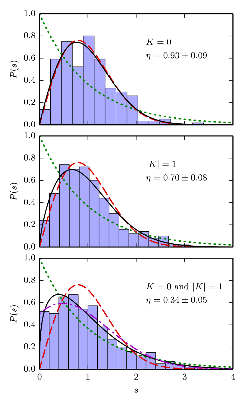
It is possible to carry out coupled-channel calculations in the body-fixed frame, neglecting the Coriolis terms off-diagonal in . This makes the problem block-diagonal and is known as helicity decoupling; it is often an effective technique for calculations of atom-diatom bound states Hutson (1991). Figure 5(a) and (b) show NNS distributions for the separate and blocks. There is no further hidden symmetry and so the NNS distributions are once again close to the Wigner-Dyson limit. Figure 5(c) shows the statistics for the superposition of the two individual level sequences. This last case is close to that of two GOE level sequences which overlap but are not coupled. The resulting NNS distribution can be obtained from equation (3.69) of Guhr et al. (1998), and is also shown in Fig. 5(c). It differs from the Wigner-Dyson distribution most obviously in that it does not vanish at zero spacing. It is in good agreement with the results from helicity decoupling calculations and explains the qualitative behavior of the distributions in Fig. 4.
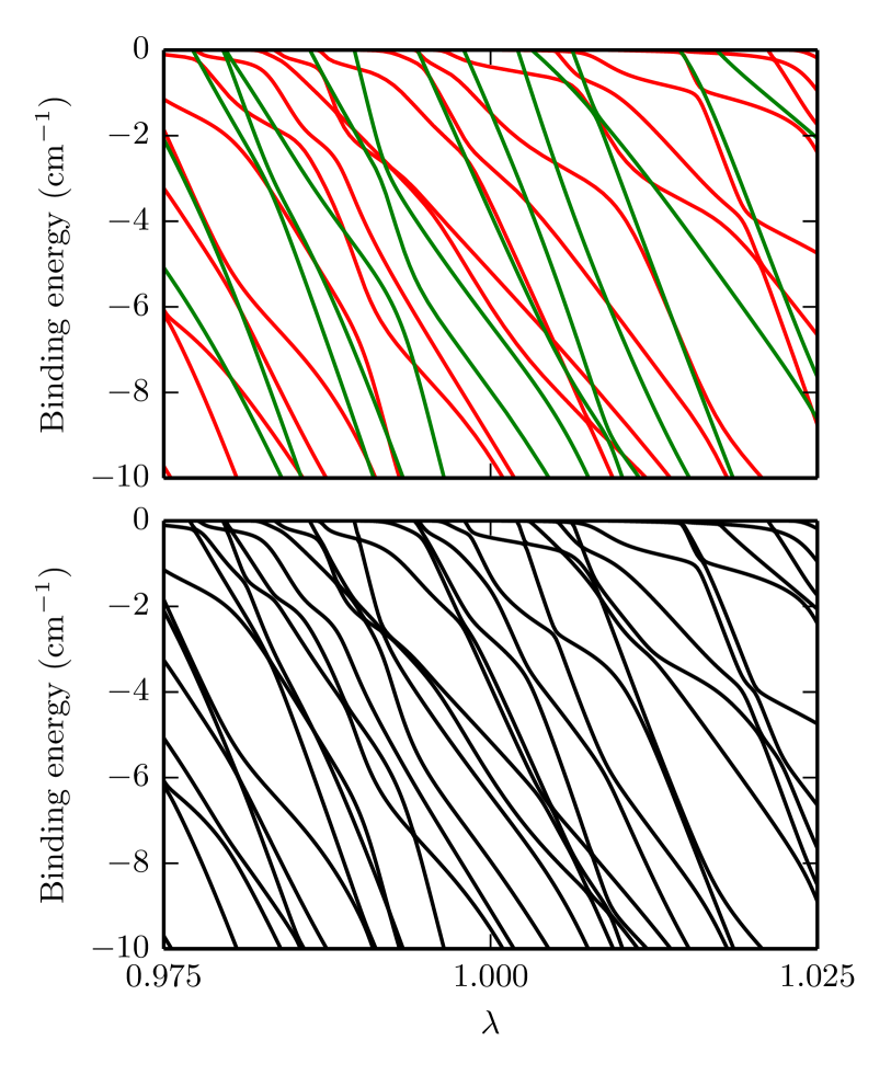
The remaining differences between Fig. 4(a) and Fig. 5(c) are due to the Coriolis terms. The quantitative effect of these terms on the statistics is beyond the scope of this paper, but it is nevertheless informative to look at the pattern of bound states near threshold. Figure 6 shows bound states for within 10 cm-1 of threshold for a small range of , both from a full calculation and within the helicity decoupling approximation. The levels for are only slightly shifted from the levels for (top panel of Fig. 3). The levels are quite different but show the same qualitative features of many avoided crossings of a wide variety of strengths. However, in the helicity decoupling approximation, levels with one value of do not interact with those of different ; this gives rise to a large number of true crossings, producing an NNS distribution with finite probability at zero spacing. In the full calculation, which takes account of the Coriolis coupling between the blocks, the overall pattern of levels is similar but there are now narrow avoided crossings between levels of different . These are typically much narrower than those between levels of the same . This confirms our picture of a nearly conserved quantum number, with only weak coupling between states of different .
IV.2 Li+CaF
The second system we consider is Li+CaF. The rotational constant for CaF is about 13 times smaller than that for CaH, while the potential surface is quite similar. The ratio of the anisotropy to is thus significantly greater for CaF than for CaH. This stronger effective coupling might be expected to give equal or greater amounts of chaos for Li+CaF compared to Li+CaH.
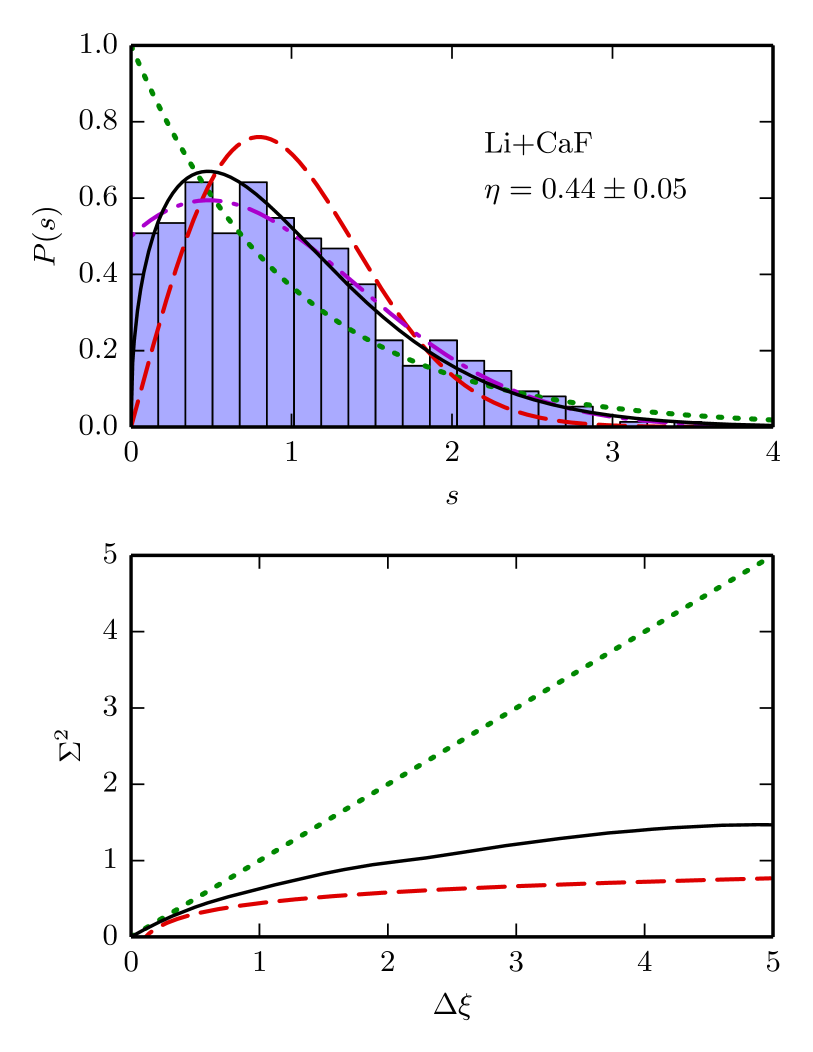
We have performed coupled-channel calculations for Li+CaF () using the same methods as for Li+CaH, but with a larger basis set because of the smaller value of . Figure 7 shows the resulting level statistics. Remarkably, the NNS distribution does not appear to show level repulsion, even for , but neither does it resemble a Poisson distribution; the fitted Brody parameter is only 0.44. Once again the distribution bears a close resemblance to the case of two overlapping but non-interacting GOE spectra as discussed for the helicity-decoupled case for Li+CaH. This again hints at the possibility of some unexpected partially good quantum number, but in this case it cannot be the projection . The level number variance for Li+CaF (=0) is also some way from the GOE prediction, although it does level off at high spacings, in contrast to that in other near-chaotic examples Maier et al. (2015b); Jachymski and Julienne (2015).
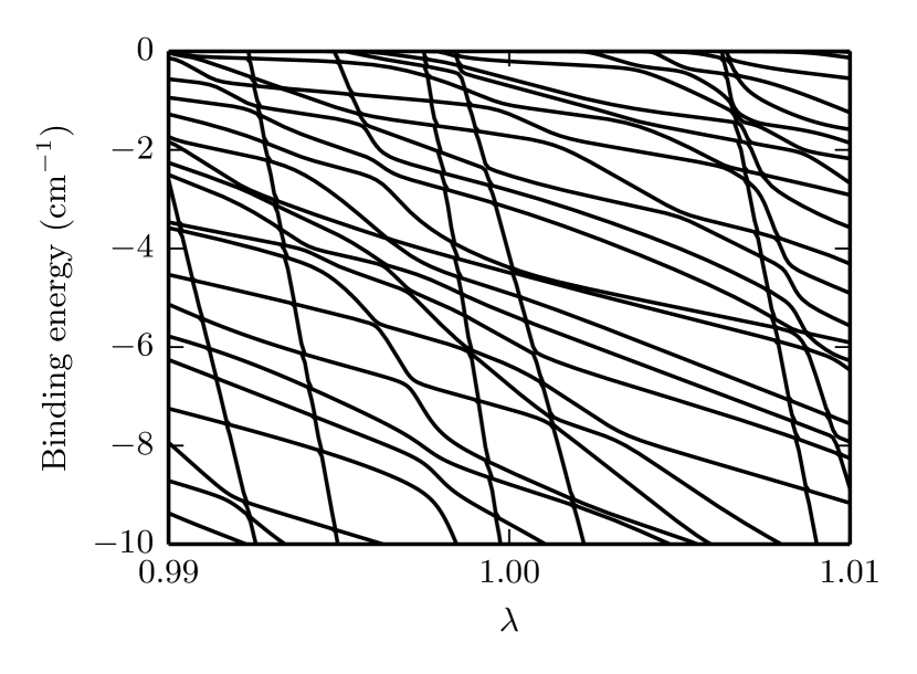
Figure 8 shows the binding energies of near-threshold levels for Li+CaF () as a function of . It may be seen that some bound states have very steep energy gradients with respect to and that these states interact weakly with those with shallower gradients 444Although visually there may seem to be relatively few steep states for Li+CaF, counting them with respect to at fixed energy reveals that approximately 1/3 of the levels are of this type.. In this respect the pattern shows a clear systematic difference from that observed for Li+CaH (Fig. 3), where all states appeared significantly coupled and the levels could not easily be separated into classes.
There has been a great deal of work on the energy levels of atom-diatom systems, largely aimed at understanding the dynamics of Van der Waals complexes Hutson (1991). For low anisotropies, the diatomic molecule executes hindered rotation in the complex, and the resulting internal rotation is only weakly coupled to the intermolecular stretching motion. However, when the effective anisotropy is comparable to or larger than the diatom rotational constant, there is significant mixing of diatom rotational states. As the anisotropy increases further, the internal rotation is transformed into a bending vibration of the triatomic molecule. Correlation diagrams showing how this transition occurs have been given in ref. Hutson, 1991 for complexes with both linear and non-linear equilibrium geometries. The low-lying levels of a non-linear species such as Li-CaH or Li-CaF eventually execute low-amplitude bending vibrations about their non-linear equilibrium. The degree of mixing between bending and stretching degrees of freedom typically depends on their relative frequencies: if the bending is either much faster or much slower than the stretching then the modes can be separated in a Born-Oppenheimer sense Holmgren et al. (1977); Hutson and Howard (1980, 1982), but if the frequencies are comparable then they are strongly mixed.
The situation is more complicated for highly excited states, such as the near-dissociation states that give rise to Feshbach resonances in the present work. Some highly excited states have unstructured nodal patterns that fill the energetically accessible space, but there are others with simple nodal patterns that sample restricted regions of space Le Sueur et al. (1993); de Polavieja et al. (1994); Wright and Hutson (1999, 2000). However, the paths along which such states are localized may be complicated ones that do not correspond to obvious quantum numbers. Because of this, it may be difficult to identify the specific nearly conserved quantity that divides the states in Fig. 8 into separate classes. Nevertheless, the level statistics appear to indicate that such a quantity exists.
IV.3 Variable rotational constant
To understand better the puzzling difference between Li+CaH and Li+CaF, we attempt to interpolate between our two systems and extrapolate beyond them. Since the two potential energy surfaces are so similar, we use the surface and reduced mass for Li+CaH throughout this section, and vary the rotational constant. We increase the number of rotational basis functions from 55 to 350 as decreases from 100 to 0.01 cm-1 to obtain converged level positions.
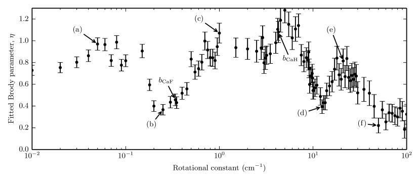
Figure 9 shows the fitted Brody parameter as a function of rotational constant. This shows an astonishing structure. It can be seen that lies in a relatively wide region from 0.7 to 7 cm-1 where is near unity, so that the systems can be said to be chaotic. Towards lower rotational constant the fitted Brody parameter falls sharply to about 0.4 in the region between 0.2 and 0.4 cm-1 – in which lies – but it then rises rapidly back to values near unity for 0.05 cm cm-1 before beginning to fall slowly again. At higher values of , there is another steep and narrow trough centered around 12 cm-1, followed by a steady decrease towards zero as the angular and radial motions become increasingly uncoupled.
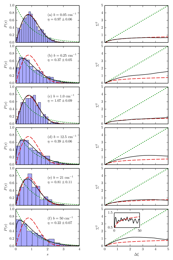
Figure 10 shows statistics for sample values of the rotational constant . Those for the lowest value, cm-1 [Fig. 10(a)] show almost perfect agreement with the GOE predictions for both NNS distribution and level number variance; the fitted Brody parameter is . The second value, cm-1, is close to cm-1, but the NNS distribution [Fig. 10(b)] differs from that seen for Li+CaF in Fig. 7(a), with noticeably more level repulsion despite a lower . cm-1 [Fig. 10(c)] is within the same region of high as and also shows clear signs of chaos. cm-1 [Fig. 10(d)] is located in a narrow trough of low and the statistics appear to be similar to case (b). cm-1 [Fig. 10(e)] is located above the trough in ; the Brody parameter is only 0.8 but the statistics show all the qualitative features expected of a chaotic system. The statistics for cm-1 [Fig. 10(f)] show an NNS distribution that is close to Poissonian () because the rotational constant is large enough for the rotational and stretching motions to be significantly decoupled and the conditions for chaos no longer exist. However, the number variance does not rise linearly as in the Poisson case; instead it reaches a peak and turns downwards. The inset shows that, on a larger scale, this is the first in a complex series of oscillations, which we attribute to the onset of regularity and do not interpret further in this paper.
The presence of oscillations in the Brody parameter in Fig. 9 is puzzling. The argument given in section IV.2 above would predict a single maximum in the Brody parameter when the effective bending and stretching frequencies are comparable for near-threshold states, dropping off when the frequencies are very different. Fig. 9 does appear to show such a maximum, but the argument does not explain the deep minima that seem to be present either side of it. It is possible that the flanking maxima correspond to effective bending frequencies that match the stretching frequencies for different stretching states, or that are rational multiples of effective stretching frequencies.
V Conclusions
We have carried out calculations on threshold and near-threshold bound states of atom + rigid-rotor models of Li+CaH and Li+CaF, and performed statistical analysis of the resulting level sequences. For Li+CaH with zero total angular momentum we have found the strongest signs of chaos yet observed for a realistic ultracold collision system in either theory or experiment. However, for non-zero total angular momentum we found a nearly good quantum number which we identified as the body-fixed projection of the total angular momentum . The presence of this nearly conserved quantity significantly alters the overall statistics, but the statistics for individual values of still show chaotic behavior. The superposition of two nearly independent level sequences in the case produces an NNS distribution that is distinct from the Poisson, Wigner-Dyson and Brody distributions.
The ratio of the anisotropy to the diatom rotational constant is significantly larger for Li+CaF than for Li+CaH. Nevertheless, contrary to expectation, Li+CaF shows less strongly chaotic behavior even for . The similarity of the statistics with the case of Li+CaH () suggests the presence of another nearly good quantum number in Li+CaF. The emergence of this quantum number may be related to an adiabatic separation between a slow bending vibration and a faster intermolecular stretch.
Finally, we have investigated how the statistics change between and beyond our two systems by varying the rotational constant with a fixed potential. We observe astonishing fluctuations in the levels of chaos in the system. It thus cannot even be assumed that a system that is partway between two closely related chaotic systems will itself be chaotic. The origin of this surprising effect is unclear. One possibility is that stronger chaos emerges when the bending and stretching frequencies are close to rational multiples of one another.
This study has demonstrated that the relationship between coupling strength and chaos is complicated. Starting from a chaotic system and increasing the strength of a coupling does not necessarily lead to an increase in chaos. This should not be surprising in principle: if a single term in a hamiltonian becomes dominant, that term defines nearly good quantum numbers for the system. The superposition of nearly independent level sequences for different values of the nearly good quantum numbers then produces non-chaotic statistics.
It is clear that there is much to be learned from studying chaos in ultracold collisions and high-lying bound states of atoms and molecules. Statistical analysis can provide valuable insight when the spectra are too complex for direct analysis. However, this study has highlighted that deviations from chaotic behavior can be difficult to predict, even in apparently simple systems. Future work will focus on the origins of chaotic and non-chaotic statistics in increasingly complex systems. One question of particular importance is whether, in real systems, all degrees of freedom are involved in the chaotic behavior, or whether there is a hierarchy of couplings that leaves some degrees of freedom uninvolved. Our results for Li+CaH () represent a particularly simple example of a case with a clear hierarchy.
Acknowledgements.
This work has been supported by the UK Engineering and Physical Sciences Research Council (grant EP/I012044/1). The authors are grateful to Timur Tscherbul, Jacek Kłos and Alexei Buchachenko for supplying the potential energy surface used for Li+CaH.References
- Chin et al. (2010) C. Chin, R. Grimm, E. Tiesinga, and P. S. Julienne, “Feshbach resonances in ultracold gases,” Rev. Mod. Phys. 82, 1225 (2010).
- Takekoshi et al. (2012) T. Takekoshi, M. Debatin, R. Rameshan, F. Ferlaino, R. Grimm, H.-C. Nägerl, C. R. Le Sueur, J. M. Hutson, P. S. Julienne, S. Kotochigova, and E. Tiemann, “Towards the production of ultracold ground-state RbCs molecules: Feshbach resonances, weakly bound states, and coupled-channel models,” Phys. Rev. A 85, 032506 (2012).
- Berninger et al. (2013) M. Berninger, A. Zenesini, B. Huang, W. Harm, H.-C. Nägerl, F. Ferlaino, R. Grimm, P. S. Julienne, and J. M. Hutson, “Feshbach resonances, weakly bound molecular states and coupled-channel potentials for cesium at high magnetic field,” Phys. Rev. A 87, 032517 (2013).
- Julienne and Hutson (2014) P. S. Julienne and J. M. Hutson, “Contrasting the wide Feshbach resonances in 6Li and 7Li,” Phys. Rev. A 89, 052715 (2014).
- Frantzeskakis (2010) D. J. Frantzeskakis, “Dark solitons in atomic Bose-Einstein condensates: from theory to experiments,” J. Phys. A 43, 213001 (2010).
- Köhler et al. (2006) T. Köhler, K. Góral, and P. S. Julienne, “Production of cold molecules via magnetically tunable Feshbach resonances,” Rev. Mod. Phys. 78, 1311 (2006).
- Kraemer et al. (2006) T. Kraemer, M. Mark, P. Waldburger, J. G. Danzl, C. Chin, B. Engeser, A. D. Lange, K. Pilch, A. Jaakkola, H. C. Nägerl, and R. Grimm, “Evidence for Efimov quantum states in an ultracold gas of caesium atoms,” Nature 440, 315 (2006).
- Huang et al. (2014) B. Huang, L. A. Sidorenkov, R. Grimm, and J. M. Hutson, “Observation of the second triatomic resonance in Efimov’s scenario,” Phys. Rev. Lett. 112, 190401 (2014).
- Lu et al. (2011) M. Lu, N. Q. Burdick, S. H. Youn, and B. L. Lev, “Strongly dipolar Bose-Einstein condensate of dysprosium,” Phys. Rev. Lett. 107, 190401 (2011).
- Pasquiou et al. (2012) B. Pasquiou, E. Maréchal, L. Vernac, O. Gorceix, and B. Laburthe-Tolra, “Thermodynamics of a Bose-Einstein condensate with free magnetization,” Phys. Rev. Lett. 108, 045307 (2012).
- Aikawa et al. (2012) K. Aikawa, A. Frisch, M. Mark, S. Baier, A. Rietzler, R. Grimm, and F. Ferlaino, “Bose-Einstein condensation of erbium,” Phys. Rev. Lett. 108, 210401 (2012).
- Baumann et al. (2014) K. Baumann, N. Q. Burdick, M. Lu, and B. L. Lev, “Observation of low-field Fano-Feshbach resonances in ultracold gases of dysprosium,” Phys. Rev. A 89, 020701 (2014).
- Maier et al. (2015a) T. Maier, I. Ferrier-Barbut, H. Kadau, M. Schmitt, M. Wenzel, C. Wink, T. Pfau, K. Jachymski, and P. S. Julienne, “Broad universal Feshbach resonances in the chaotic spectrum of dysprosium atoms,” Phys. Rev. A 92, 060702 (2015a).
- Frisch et al. (2015) A. Frisch, M. Mark, K. Aikawa, S. Baier, R. Grimm, A. Petrov, S. Kotochigova, G. Quéméner, M. Lepers, O. Dulieu, and F. Ferlaino, “Ultracold dipolar molecules composed of strongly magnetic atoms,” Phys. Rev. Lett. 115, 203201 (2015).
- Ni et al. (2008) K.-K. Ni, S. Ospelkaus, M. H. G. de Miranda, A. Pe’er, B. Neyenhuis, J. J. Zirbel, S. Kotochigova, P. S. Julienne, D. S. Jin, and J. Ye, “A high phase-space-density gas of polar molecules in the rovibrational ground state,” Science 322, 231 (2008).
- Ospelkaus et al. (2010) S. Ospelkaus, K.-K. Ni, D. Wang, M. H. G. de Miranda, B. Neyenhuis, G. Quéméner, P. S. Julienne, J. L. Bohn, D. S. Jin, and J. Ye, “Quantum-state controlled chemical reactions of ultracold KRb molecules,” Science 327, 853 (2010).
- Parazzoli et al. (2011) L. P. Parazzoli, N. J. Fitch, P. S. Żuchowski, J. M. Hutson, and H. J. Lewandowski, “Large effects of electric fields on atom-molecule collisions at millikelvin temperatures,” Phys. Rev. Lett. 106, 193201 (2011).
- Takekoshi et al. (2014) T. Takekoshi, L. Reichsöllner, A. Schindewolf, J. M. Hutson, C. R. Le Sueur, O. Dulieu, F. Ferlaino, R. Grimm, and H.-C. Nägerl, “Ultracold dense samples of dipolar RbCs molecules in the rovibrational and hyperfine ground state,” Phys. Rev. Lett. 113, 205301 (2014).
- Molony et al. (2014) P. K. Molony, P. D. Gregory, Z. Ji, B. Lu, M. P. Köppinger, C. R. Le Sueur, C. L. Blackley, J. M. Hutson, and S. L. Cornish, “Creation of ultracold 87Rb133Cs molecules in the rovibrational ground state,” Phys. Rev. Lett. 113, 255301 (2014).
- Frisch et al. (2014) A. Frisch, M. Mark, K. Aikawa, F. Ferlaino, J. L. Bohn, C. Makrides, A. Petrov, and S. Kotochigova, “Quantum chaos in ultracold collisions of gas-phase erbium atoms,” Nature 507, 475 (2014).
- Mehta (1991) M. L. Mehta, Random Matrices, 2nd ed. (Academic Press, 1991).
- Guhr et al. (1998) T. Guhr, A. Müller-Groeling, and H. A. Weidenmüller, “Random matrix theories in quantum physics: common concepts,” Phys. Rep. 299, 189 (1998).
- Wigner (1955) E. P. Wigner, “Characteristic vectors of bordered matrices with infinite dimensions,” Ann. Math. Second Series, 62, pp. 548 (1955).
- Dyson (1962) F. J. Dyson, “Statistical theory of the energy levels of complex systems. I,” J. Math. Phys. 3, 140 (1962).
- Mayle et al. (2012) M. Mayle, B. P. Ruzic, and J. L. Bohn, “Statistical aspects of ultracold resonant scattering,” Phys. Rev. A 85, 062712 (2012).
- Mayle et al. (2013) M. Mayle, G. Quéméner, B. P. Ruzic, and J. L. Bohn, “Scattering of ultracold molecules in the highly resonant regime,” Phys. Rev. A 87, 012709 (2013).
- Maier et al. (2015b) T. Maier, H. Kadau, M. Schmitt, M. Wenzel, I. Ferrier-Barbut, T. Pfau, A. Frisch, S. Baier, K. Aikawa, L. Chomaz, M. J. Mark, F. Ferlaino, C. Makrides, E. Tiesinga, A. Petrov, and S. Kotochigova, “Emergence of chaotic scattering in ultracold Er and Dy,” Phys. Rev. X 5, 041029 (2015b).
- Jachymski and Julienne (2015) K. Jachymski and P. S. Julienne, “Chaotic scattering in the presence of a dense set of overlapping Feshbach resonances,” Phys. Rev. A 92, 020702 (2015).
- Bohigas et al. (1984) O. Bohigas, M. J. Giannoni, and C. Schmit, “Characterization of chaotic quantum spectra and universality of level fluctuation laws,” Phys. Rev. Lett. 52, 1 (1984).
- Mur-Petit and Molina (2015) J. Mur-Petit and R. A. Molina, “Spectral statistics of molecular resonances in erbium isotopes: How chaotic are they?” Phys. Rev. E 92, 042906 (2015).
- Green et al. (2016) D. G. Green, C. L. Vaillant, M. D. Frye, M. Morita, and J. M. Hutson, “Quantum chaos in ultracold collisions between and ,” Phys. Rev. A 93, 022703 (2016).
- González-Martínez and Żuchowski (2015) M. L. González-Martínez and P. S. Żuchowski, “Magnetically tunable Feshbach resonances in Li+Er,” Phys. Rev. A 92, 022708 (2015).
- Bernstein (1979) R. B. Bernstein, ed., Atom-Molecule Collision Theory: a Guide for the Experimentalist (Plenum Press, New York, 1979).
- Hutson (1991) J. M. Hutson, “An introduction to the dynamics of Van der Waals molecules,” in Advances in Molecular Vibrations and Collision Dynamics, Vol. 1A (JAI Press, Greenwich, Connecticut, 1991) pp. 1–45.
- Hutson (1994) J. M. Hutson, “Coupled-channel methods for solving the bound-state Schrödinger equation,” Comput. Phys. Commun. 84, 1 (1994).
- Hutson and Green (1994) J. M. Hutson and S. Green, “MOLSCAT computer program, version 14,” distributed by Collaborative Computational Project No. 6 of the UK Engineering and Physical Sciences Research Council (1994).
- Hutson (1993) J. M. Hutson, “BOUND computer program, version 5,” distributed by Collaborative Computational Project No. 6 of the UK Engineering and Physical Sciences Research Council (1993).
- Hummon et al. (2011) M. T. Hummon, T. V. Tscherbul, J. Kłos, H.-I. Lu, E. Tsikata, W. C. Campbell, A. Dalgarno, and J. M. Doyle, “Cold N + NH collisions in a magnetic trap,” Phys. Rev. Lett. 106, 053201 (2011).
- Lu et al. (2014) H.-I. Lu, I. Kozyryev, B. Hemmerling, J. Piskorski, and J. M. Doyle, “Magnetic trapping of molecules via optical loading and magnetic slowing,” Phys. Rev. Lett. 112, 113006 (2014).
- Tscherbul et al. (2011) T. V. Tscherbul, J. Kłos, and A. A. Buchachenko, “Ultracold spin-polarized mixtures of molecules with -state atoms: Collisional stability and implications for sympathetic cooling,” Phys. Rev. A 84, 040701 (2011).
- Werner et al. (2015) H.-J. Werner, P. J. Knowles, G. Knizia, F. R. Manby, M. Schütz, P. Celani, T. Korona, R. Lindh, A. Mitrushenkov, G. Rauhut, K. R. Shamasundar, T. B. Adler, R. D. Amos, A. Bernhardsson, A. Berning, D. L. Cooper, M. J. O. Deegan, A. J. Dobbyn, F. Eckert, E. Goll, C. Hampel, A. Hesselmann, G. Hetzer, T. Hrenar, G. Jansen, C. Köppl, Y. Liu, A. W. Lloyd, R. A. Mata, A. J. May, S. J. McNicholas, W. Meyer, M. E. Mura, A. Nicklass, D. P. O’Neill, P. Palmieri, K. Pflüger, R. Pitzer, M. Reiher, T. Shiozaki, H. Stoll, A. J. Stone, R. Tarroni, T. Thorsteinsson, M. Wang, and A. Wolf, “MOLPRO, version 2010.1, a package of ab initio programs,” (2015), see http://www.molpro.net.
- Dunning (1989) T. H. Dunning, Jr., “Gaussian basis sets for use in correlated molecular calculations. I. The atoms boron through neon and hydrogen,” J. Chem. Phys. 90, 1007 (1989).
- Kendall et al. (1992) R. A. Kendall, T. H. Dunning, and R. J. Harrison, “Electron affinities of the first-row atoms revisited. Systematic basis sets and wave functions,” J. Chem. Phys. 96, 6796 (1992).
- Koput and Peterson (2002) J. Koput and K. A. Peterson, “Ab initio potential energy surface and vibrational-rotational energy levels of X CaOH,” J. Phys. Chem. A 106, 9595 (2002).
- Boys and Bernardi (1970) S. F. Boys and F. Bernardi, “The calculation of small molecular interactions by the differences of separate total energies. Some procedures with reduced errors,” Mol. Phys. 19, 553 (1970).
- Kaledin et al. (1999) L. A. Kaledin, J. C. Bloch, M. C. McCarthy, and R. W. Field, “Analysis and deperturbation of the and states of CaF,” J. Mol. Spectrosc. 197, 289 (1999).
- Brody et al. (1981) T. A. Brody, J. Flores, J. B. French, P. A. Mellow, A. Pandey, and S. S. M. Wong, “Random-matrix physics: spectrum and strength fluctuations,” Rev. Mod. Phys. 53, 385 (1981).
- Cvitaš et al. (2007) M. T. Cvitaš, P. Soldán, J. M. Hutson, P. Honvault, and J. M. Launay, “Interactions and dynamics in Li + Li2 ultracold collisions,” J. Chem. Phys. 127, 074302 (2007).
- Wallis and Hutson (2009) A. O. G. Wallis and J. M. Hutson, “Production of ultracold NH molecules by sympathetic cooling with Mg,” Phys. Rev. Lett. 103, 183201 (2009).
- Wallis et al. (2011) A. O. G. Wallis, E. J. J. Longdon, P. S. Żuchowski, and J. M. Hutson, “The prospects of sympathetic cooling of NH molecules with Li atoms,” Eur. Phys. J. D 65, 151 (2011).
- Note (1) Note that even should not be interpreted as the true potential because there are significant uncertainties in the calculated potentials.
- Hutson (2011) J. M. Hutson, “FIELD computer program, version 1,” (2011).
- Alexander and Manolopoulos (1987) M. H. Alexander and D. E. Manolopoulos, “A stable linear reference potential algorithm for solution of the quantum close-coupled equations in molecular scattering theory,” J. Chem. Phys. 86, 2044 (1987).
- Mizushima (1975) M. Mizushima, Theory of Rotating Diatomic Molecules (Wiley, New York, 1975).
- Note (2) The anisotropy considered in Ref. Maier et al. (2015b) is based entirely on dispersion effects Petrov et al. (2012). The spread of dispersion coefficients for different potential curves of Er-Er is 10% of their mean value, and that for Dy-Dy is 9% of their mean value.
- Note (3) We observe only a fraction of the total number of levels in the system, so .
- Berry and Robnik (1984) M. V. Berry and M. Robnik, “Semiclassical level spacings when regular and chaotic orbits coexist,” J. Phys. A 17, 2413 (1984).
- Izrailev (1988) F. Izrailev, “Quantum localization and statistics of quasienergy spectrum in a classically chaotic system,” Phys. Lett. A 134, 13 (1988).
- Brody (1973) T. Brody, “A statistical measure for the repulsion of energy levels,” Lett. Nuovo Cimento 7, 482 (1973).
- Barlow (1989) R. J. Barlow, Statistics: A Guide to the Use of Statistical Methods in the Physical Sciences (Wiley, 1989).
- Berry and Tabor (1977) M. V. Berry and M. Tabor, “Level clustering in the regular spectrum,” Proc. R. Soc. A 356, 375 (1977).
- Rosenzweig and Porter (1960) N. Rosenzweig and C. E. Porter, “‘Repulsion of energy levels’ in complex atomic spectra,” Phys. Rev. 120, 1698 (1960).
- Note (4) Although visually there may seem to be relatively few steep states for Li+CaF, counting them with respect to at fixed energy reveals that approximately 1/3 of the levels are of this type.
- Holmgren et al. (1977) S. L. Holmgren, M. Waldman, and W. Klemperer, “Internal dynamics of van der Waals complexes. I. Born–Oppenheimer separation of radial and angular motion,” J. Chem. Phys. 67, 4414 (1977).
- Hutson and Howard (1980) J. M. Hutson and B. J. Howard, “Spectroscopic properties and potential surfaces for atom-diatom van der Waals molecules,” Mol. Phys. 41, 1123 (1980).
- Hutson and Howard (1982) J. M. Hutson and B. J. Howard, “Anisotropic intermolecular forces. I. Rare gas-hydrogen chloride systems,” Mol. Phys. 45, 769 (1982).
- Le Sueur et al. (1993) C. R. Le Sueur, J. R. Henderson, and J. Tennyson, “Gateway states and bath states in the vibrational spectrum of H,” Chem. Phys. Lett. 206, 429 (1993).
- de Polavieja et al. (1994) G. G. de Polavieja, F. Borondo, and R. M. Benito, “Scars in groups of eigenstates in a classically chaotic system,” Phys. Rev. Lett. 73, 1613 (1994).
- Wright and Hutson (1999) N. J. Wright and J. M. Hutson, “Regular and irregular vibrational states: Localized anharmonic modes in Ar3,” J. Chem. Phys. 110, 902 (1999).
- Wright and Hutson (2000) N. J. Wright and J. M. Hutson, “Regular and irregular vibrational states: Localized anharmonic modes and transition-state spectroscopy of Na3,” J. Chem. Phys. 112, 3214 (2000).
- Petrov et al. (2012) A. Petrov, E. Tiesinga, and S. Kotochigova, “Anisotropy-induced Feshbach resonances in a quantum dipolar gas of highly magnetic atoms,” Phys. Rev. Lett. 109, 103002 (2012).