Entropies for severely contracted configuration space

Abstract

We demonstrate that dual entropy expressions of the Tsallis type apply naturally to statistical-mechanical systems that experience an exceptional contraction of their configuration space. The entropic index $\alpha>1$ describes the contraction process, while the dual index $\alpha^{\prime}=2-\alpha<1$ defines the contraction dimension at which extensivity is restored. We study this circumstance along the three routes to chaos in low-dimensional nonlinear maps where the attractors at the transitions, between regular and chaotic behavior, drive phase-space contraction for ensembles of trajectories. We illustrate this circumstance for properties of systems that find descriptions in terms of nonlinear maps. These are size-rank functions, urbanization and similar processes, and settings where frequency locking takes place.

Keywords: Physics, Statistical physics, Nonlinear physics, Nonlinear dynamical systems

1 Introduction

It is generally acknowledged that the validity of ordinary, Boltzmann-Gibbs (BG), equilibrium statistical mechanics rests on the capability of a system composed of many degrees of freedom to transit amongst its many possible configurations in a representative manner. The number of configurations of a typical statistical-mechanical system increases exponentially with its size, and when these configurations are reachable in an adequate fashion through a sufficiently long time period, the indispensable BG properties, ergodicity and mixing, are established [1]. Therefore, to explore the limit of validity of BG statistical mechanics it is relevant to look at situations where access to configuration space can be controlled to various degrees down to a residual set of vanishing measure. A classic example is that of supercooled molecular liquids where glass formation signals ergodicity breakdown [2].

Here we refer to an especially tractable family of model systems in which the effect of phase space contraction in their statistical-mechanical properties can be studied theoretically. These are low-dimensional nonlinear maps that describe the three different routes to chaos, intermittency, period doublings and quasi periodicity [3]. Because these systems are dissipative they possess families of attractors, and the dynamics of ensembles of trajectories towards these attractors constitute realizations of phase space contraction. When the attractors are chaotic the contraction reaches a limit in which the contracted space has the same dimension as the initial space, a set of real numbers. But when the attractor is periodic the contraction is extreme and the final number of accessible configurations is finite. When the attractors at the transitions to chaos are multifractal sets contraction leads to more involved intermediate cases. Chaotic attractors have ergodic and mixing properties but those at the transitions to chaos do not [4]. We consider them here to discuss their association with generalized entropies.

The dynamical properties imposed by the attractors at the mentioned transitions to (or out of) chaos in low-dimensional nonlinear maps can be easily determined [5] and it is our purpose to describe these properties in terms of phase space contraction. Interestingly, these contractions are found in all cases to be analytically expressed in terms of the so-called deformed exponential function, $\exp_{q}(x)\equiv\left[1+(1-q)x\right]^{1/(1-q)}$, $1\leq q\leq 2$, and these in turn, as we describe below, appear associated with dual entropy expressions via the inverse function, the deformed logarithm, $\ln_{q}(x)\equiv(1-q)^{-1}[x^{1-q}-1]$. The entropy expressions are of the Tsallis type [6], i.e.,

$$S_{1}[p_{k}]=\sum_{k=0}^{k_{\max}}p_{k}\ln_{\alpha}\,p_{k}^{-1},$$ (1)

and

$$S_{2}[p_{k}]=-\sum_{k=0}^{k_{\max}}p_{k}\ln_{\alpha^{\prime}}p_{k},$$ (2)

where $p_{k}$ are probabilities. The dual entropy expressions satisfy a maximum entropy principle (MEP) and their values coincide, $S_{2}[p_{k}]=S_{1}[p_{k}]$, when the deformation indexes obey $\alpha^{\prime}=2-\alpha<1$. The dynamics towards the attractor is measured by the index $\alpha$, whereas the index $\alpha^{\prime}$ characterizes the contraction achieved by the attractor. Absence of (effective) contraction implies $\alpha=\alpha^{\prime}=1$ and total contraction is signaled by $\alpha=2$ and $\alpha^{\prime}=0$. We define a contraction dimension via the index $\alpha^{\prime}$,

$$\alpha^{\prime}=\frac{\ln\pi_{k}}{\ln p_{k}},$$ (3)

where $\pi_{k}$ and $p_{k}$ are, respectively, the probabilities associated with the contracted set and the initial set of configurations.

In the following sections we describe the effect of phase space contraction for the three routes to chaos that occur in nonlinear maps $f(x)$ of a single variable $x$, $f$ and $x$ real numbers. We consider the effect of attractors at the transitions to chaos on ensembles of initial conditions that occupy fully one-dimensional intervals. We begin first with the simplest case of the tangent bifurcation associated with intermittency of type I [3], for which the ensemble contracts into a finite set of points. This is the most extreme situation that leads (in general) to $\alpha=2$ and $\alpha^{\prime}=0$ [7], and we corroborate this case with ranked data for forest fire sizes. Next we consider the accumulation point of period-doubling bifurcations in quadratic maps, where contraction into the most open region of the multifractal attractor leads to $\alpha\simeq 1.7555$ and $\alpha^{\prime}\simeq 0.2455$ [8]. We refer to systems where period doubling is observed or to processes modeled by quadratic maps. Finally, we look at the quasi-periodic transition to chaos in the circle map along the golden-mean route and its chosen representative region yields $\alpha\simeq 1.9489$ and $\alpha^{\prime}\simeq 0.0510$ [9]. We describe this contraction in terms of its mode-locking property [3] widely observed elsewhere.

2 Tangent bifurcation

A common account of the tangent bifurcation, that mediates the transition between a chaotic attractor and an attractor of period $n$, starts with the composition $f^{(n)}(x)$ of a one-dimensional map $f(x)$, e.g. the logistic map, at such bifurcation, followed by an expansion around the neighborhood of one of the $n$ points tangent to the line with unit slope [3]. That is

$$x^{\prime}=f^{(n)}(x)=x+ux^{z}+\cdots,\;x\geq 0,\;z>1,$$ (4)

where $x^{z}\equiv sign(x)\left|x\right|^{z}$. The functional composition Renormalization Group (RG) fixed-point map is the solution $f^{\ast}(x)$ of

$$f^{\ast}(f^{\ast}(x))=\lambda^{-1}f^{\ast}(\lambda x)$$ (5)

together with a specific value for $\lambda$ that upon expansion around $x=0$ reproduces Eq. (4). An exact analytical expression for $x^{\prime}=f^{\ast}(x)$ was obtained long ago [3]. This is

$$x^{\prime 1-z}=x^{1-z}+(1-z)u$$ (6)

or, equivalently,

$$x^{\prime}=x\exp_{z}(ux^{z-1}),$$ (7)

with $\lambda=2^{1/(z-1)}$. Repeated iteration of Eq. (6) leads to

$$x_{t}^{1-z}=x_{0}^{1-z}+(1-z)ut$$ (8)

or

$$\ln_{z}x_{t}=\ln_{z}x_{0}+ut.$$ (9)

So that the iteration number or time $t$ dependence of all trajectories is given by

$$x_{t}=x_{0}\exp_{z}\left[x_{0}^{z-1}ut\right],$$ (10)

where the $x_{0}$ are the initial positions. In Fig. 1a we plot the map in Eq. (7) when $z=2$ together with two trajectories initiated at $x_{0}<1$ and $x_{0}>1$, that in the insets are shown as functions of $t$ (also reproduced by Eq. (10)). The $q$-deformed properties of the tangent bifurcation are discussed at greater length in Ref. [7]. An ensemble of trajectories with initial conditions $x_{0}$ distributed within an interval $X\leq x_{0}<0$, $X<0$ arbitrary, undergoes progressive phase space contraction ending up into the point $x=0$.

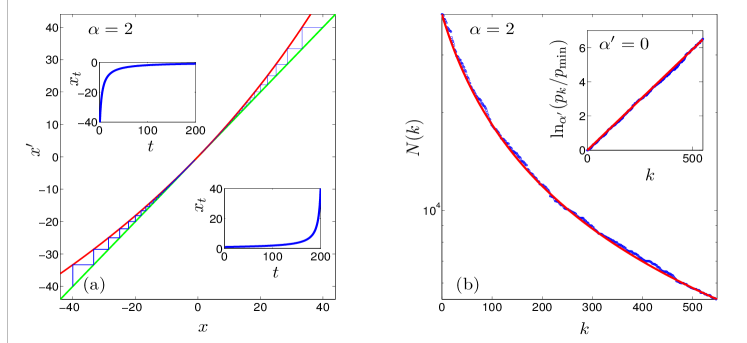
Figure 1: (a) The map in Eq. (7) with $z=2$ and $u=-0.005$ (red), two trajectories are shown with $x_{0}<0$ and $x_{0}>0$ (blue). The insets show the time dependence of these trajectories that obey Eq. (10). (b) Rank-order statistics for the occurrence of forest fires (blue dots) from Ref. [13]. They are reproduced by the smooth curve from Eq. (11) with $\alpha=2$ and $\mathcal{N}^{-1}=-u$ (red). The inset shows the same data (blue) plotted in $\ln_{\alpha^{\prime}}(p_{k}/p_{\min})$ scale, $p_{k}=1/N(k)$ and $\alpha^{\prime}=0$. The straight line is the corresponding plot of Eq. (12) (red) and evidences the extensivity of the entropy in Eq. (13). See text for details.

Interestingly, a manifestation of the dynamical properties at the tangent bifurcation appears in ranked data that follow Zipf’s law for large enough rank. It has been shown [10], [11] that size-rank functions, as given by a basic argument [12] that generalizes Zipf’s law, are strictly analogous to the RG fixed-point map trajectories in Eq. (10). The expression for the size-rank function $N(k)$, the magnitude of the data $N$ for rank $k$,

$$N(k)=N_{\max}\exp_{\alpha}[-N_{\max}^{\alpha-1}\mathcal{N}^{-1}k],$$ (11)

where $\mathcal{N}=k_{\max}$ is the total number of data, becomes that in Eq. (10) with the identifications $k=t$, $\mathcal{N}^{-1}=-u$, $N(k)=-x_{t}$, $N_{\max}=-x_{0}$ and $\alpha=z$. We note that the most common value for the degree of nonlinearity at tangency is $z=2$, obtained when the map is analytic at $x=0$ with nonzero second derivative, and this implies $\alpha=2$, close to the values observed for many sets of real data, as this conforms with the classical Zipf’s law form $N(k)\sim k^{-1}$ when $k$ is large. The inverse of $N(k)$, $p_{k}=1/N(k)$, the (uniform) probability for the occurrence of each unit that constitutes $N(k)$, is given by

$$p_{k}=p_{\min}\exp_{\alpha^{\prime}}(p_{\min}^{\alpha^{\prime}-1}\mathcal{N}^{-1}k),$$ (12)

where $p_{\min}=1/N_{\max}$. In Fig. 1b we plot $N(k)$ in Eq. (11) when $\alpha=2$ together with ranked data of forest fires areas [13] while in the inset we plot Eq. (12) when $\alpha^{\prime}=0$ also with the corresponding forest fire data. We notice that, if $W(k_{\max})\equiv N_{\max}/{N(k_{\max})}$ is identified as the number of configurations of the system of size equal to the maximum rank $k_{\max}$ that generates the data set $N(k),k=0,1,\ldots,k_{\max}$, then from Eq. (12) we observe that the size-dependent entropy [14]

$$S(k_{\max})\equiv\ln_{\alpha^{\prime}}W(k_{\max}),$$ (13)

is extensive.

3 Period-doubling accumulation point

The classic example of functional composition RG fixed-point map is the solution of Eq. (5) associated with the period-doubling accumulation points of unimodal maps [3]. In practice it is often illustrated by use of the quadratic $z=2$ logistic map $f_{\mu}(x)=1-\mu x^{2}$, $-1\leq x\leq 1$, $0\leq\mu\leq 2$, with the control parameter located at $\mu=\mu_{\infty}(z=2)=1.401155189092\cdots$, the value for the accumulation point of the main period-doubling cascade [4]. The scaling factor, known as Feigenbaum’s universal constant, is $\lambda(z=2)=-2.50290\cdots$ (for convenience we denote below its absolute value with the same symbol).

Fig. 2a shows two features of the trajectory at $\mu_{\infty}(z=2)$ with initial condition at $x_{0}=0$ that are relevant to our discussion. Notice that in this figure we have used absolute values of iterated positions $\left|x_{t}\right|$ to facilitate the use logarithmic scales. The labels correspond to iteration times $t$. The first visible feature in the figure is that the positions fall within equally-spaced horizontal bands. Since all positions visited at odd times form the top band one half of the attractor lies there. Inspection of the iteration times for positions within the subsequent bands indicates that one quarter of the attractor forms the second band, one eighth the third band, and so on. Repeated functional composition of the unimodal map eliminates bands successively starting with the top band, and these in turn can be recovered (approximately) by repeated rescaling by a factor equal to $\lambda$. This removal and recuperation of bands correspond to a graphical construction of the functional composition and rescaling of the RG transformation.

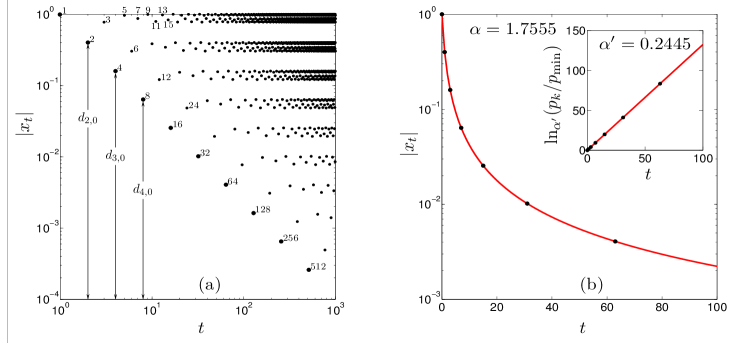
Figure 2: (a) Absolute value of trajectory positions $x_{t}$, $t=0,1,\ldots$, for the logistic map $f_{\mu}(x)$ at $\mu_{\infty}$, with initial condition $x_{0}=0$, in logarithmic scale as a function of the logarithm of the time $t$, also shown by the numbers close to the points. The arrows indicate the distances equivalent to the principal diameters $d_{n,0}$. (b) The positions $\left|x_{t}\right|$ of the trajectory in (a) at selected iteration times $t=2^{n}-1$ (black dots) reproduced by Eq. (14) with $\alpha=1.7555$ (red). The inset shows the same data plotted in $\ln_{\alpha^{\prime}}p_{k}/p_{\min}$ scale, $p_{k}=1/\left|x_{k}\right|$, $p_{\min}=1$ and $\alpha^{\prime}=0.2445$. The straight line evidences the (time) extensivity of the entropy in Eq. (13). See text for description.

The second feature evident in Fig. 2a is that all the attractor positions fall into a well-defined family of straight diagonal lines, all with the same slope. All the attractor positions can be allocated into subsequences formed by the time subsequences $t=(2k+1)2^{n}-1$, with $n=0,1,2,\ldots$ and fixed $k=0,1,2,\ldots$. Thus, the subsequences $\left|x_{t}\right|$ have each a common power-law decay $\left|x_{t}\right|\simeq(t+1)^{1/1-\alpha}$, with $\alpha=1+\ln 2/\ln\lambda(z)$, $\alpha\simeq 1.7555$ when $z=2$ [5], [8]. Interestingly, these subsequences can be seen [5], [8] to reproduce the positions of the so-called ‘superstable’ periodic trajectories [3]. In particular, the positions for the main subsequence $k=0$ are given by $\left|x_{2^{n-1}}\right|\simeq d_{n,0}=$ $\lambda^{-n}$, where $d_{n,0}\equiv\left|f_{\overline{\mu}_{n}}^{(2^{n-1})}(0)\right|$ is the ‘$n$-th principal diameter’ [3]. With use of $\lambda^{-n}\equiv(1+t)^{-\ln\lambda/\ln 2}$, $t=2^{n}-1$, this subsequence can be expressed as

$$\left|x_{t}\right|=\exp_{\alpha}(-\Lambda_{\alpha}t)$$ (14)

with $\alpha$ as above and $\Lambda_{\alpha}=(z-1)\ln\lambda/\ln 2$. See [5], [8].

The band structure in Fig. 2a involves families of phase-space gaps that decrease in width as power laws (equal sizes in logarithmic scales of the figure). These gaps are formed sequentially, beginning with the largest one, in the dynamics towards the attractor at $\mu_{\infty}$. This process has a hierarchical organization and can be observed explicitly by placing an ensemble of initial conditions $x_{0}$ distributed uniformly across phase space and record their positions at subsequent times [5, 15, 16]. The main gaps in Fig. 2a decrease with the same power law of the principal diameters $d_{n,0}$ described above and expressed as the deformed exponential in Eq. (14). The locations of this specific family of consecutive gaps advance monotonically toward the sparsest region of the multifractal attractor located at $x=0$ [5, 8, 15]. The decreasing values of $\left|x_{t}\right|$, $t=2^{n}-1$ in Eq. (14) with increasing $n$, describe phase-space contraction along iteration time evolution as these intervals represent the widths of the gaps forming consecutively, the diameter $d_{n,0}$ being the width of the gap formed after $t=2^{n+1}-1$ [15]. Similarly other families of diameters represent widths of gaps leading to the multifractal attractor. In Fig. 2b we plot Eq. (14) with $\alpha\simeq 1.7555$ that reproduces the positions $x_{t}$ of the trajectory initiated at $x_{0}$ for iteration times $t=2^{n}-1$, $n=0,1,2,\ldots$. In the inset we plot $\ln_{\alpha^{\prime}}p_{k}$, $p_{k}=1/\left|x_{k}\right|$ with $\alpha^{\prime}=2-\alpha=0.2445$. The straight line corresponds to Eq. (13) (with $p_{\min}=1$ and $\mathcal{N}=\ln 2/\ln\lambda)$ in Eq. (12), and corroborates the (time) extensivity of entropy.

4 Golden-mean route to chaos

The quasi periodic route to chaos is often studied by means of the circle map,

$$f_{\Omega,K}(\theta)=\theta+\Omega-K/(2\pi)\sin 2\pi\theta,\;\textnormal{mod}\;1,$$ (15)

where the control parameters $\Omega$ and $K$ are, respectively, the bare winding number and the degree of nonlinearity [3]. Another quantity relevant to the dynamics generated by this map is the dressed winding number $\omega\equiv\lim_{t\rightarrow\infty}[\theta_{t}-\theta_{0}]/t$. Locked motion (a periodic attractor) occurs when $\omega$ is rational and unlocked motion (a quasi periodic attractor) when $\omega$ is irrational. We are interested in the critical circle map $K=1$ when locked motion occurs for all $\Omega$, $0\leq\Omega\leq 1$, except for a multifractal set of unlocked values. Sequences of locked motion values of $\Omega$ can be used to select attractors of increasing periods such that a transition to chaos is obtained at their infinite-period (quasi periodic) accumulation points [3].

A well-known specific case of the above is the sequence of rational approximations to the reciprocal of the golden mean $\omega_{\rm gm}=(\sqrt{5}-1)/2\simeq 0.618034$. This sequence is formed by the winding numbers $\omega_{n}=F_{n-1}/F_{n}$, where $F_{n}$ are the Fibonacci numbers $F_{n+1}=$ $F_{n}+F_{n-1}$. The route to chaos is the family of attractors with increasing periods $F_{n}$, $n\rightarrow\infty$. Amongst these attractors it is possible to select specific values of $\Omega$ with the superstable property [3]. As before, a superstable trajectory of period $T$ satisfies $df^{(T)}(\theta_{0})/d\theta=0$, and is one that contains as one of its positions $\theta=0$. There are two superstable families of trajectories, the first at control parameter values $\Omega_{n}$, $n=1,2,\ldots$ with winding numbers $\omega_{n}=F_{n-1}/F_{n}$ and accumulation point at $\Omega_{\infty}\simeq 0.606661$ which corresponds to $\omega_{\rm gm}$. The second family with winding numbers $\omega_{n}^{\prime}=F_{n-2}/F_{n}$, with $\Omega_{n}^{\prime}$, $n=1,2,\ldots$ and accumulation point at $\Omega_{\infty}^{\prime}=1-\Omega_{\infty}\simeq 0.393339$ which corresponds to $\omega_{\rm gm}^{2}\simeq\allowbreak 0.381966$ [9].

As with the period-doubling route, the quasiperiodic route to chaos displays universal scaling properties. And an RG approach, analogous to that for the tangent bifurcation and the period doubling cascade, has been carried out for the critical circle map [3]. The fixed-point map $f^{\ast}(\theta)$ of an RG transformation that consists of functional composition and rescaling appropriate for maps with a zero-slope cubic inflection point (like the critical circle map) satisfies

$$f^{\ast}(\theta)=\lambda_{\rm gm}f^{\ast}(\lambda_{\rm gm}f^{\ast}(\theta/\lambda_{\rm gm}^{2})),$$ (16)

where (for the golden mean route) $\lambda_{\rm gm}\simeq-1.288575$ is a universal constant [3]. (We denote below its absolute value with the same symbol). This constant describes the scaling of the distance $d_{n,0}$ from $\theta=0$ to the nearest element of the orbit with $\omega_{n}$. These are the distances analogous to the principal diameters in the previous section [3].

For our purposes we refer only to one family of winding numbers, $\omega_{n}^{\prime}=F_{n-2}/F_{n}$. Fig. 3a shows the trajectory at $\Omega=\Omega_{\infty}^{\prime}$ starting at $\theta_{0}=0$ in logarithmic scales where the labels indicate iteration times $t$. Similarly to Fig. 2a, a conspicuous feature in Fig. 3a is that positions fall along straight diagonal lines, again, a signal of multiple power law behavior. Notice that the positions of the main diagonal in Fig. 3a correspond to the times $F_{2n}$, $n=1,2,3,\ldots$ The succeeding diagonals above it appear grouped together (see Ref. [9] for a description). Also similarly to Fig. 2a, in Fig. 3a we show the positions for the main subsequence that constitutes the lower bound of the entire trajectory. These positions are identified to be $\theta_{F_{2n}}\simeq d_{2n,0}=\Omega_{\infty}^{\prime}\lambda_{\rm gm}^{-2n}$, where $d_{2n,0}$ is the ‘$2n$-th principal diameter’ defined at the $F_{2n}$-supercycle, the distance of the orbit position nearest to $\theta=0$ [3], [9]. With use of $\lambda_{\rm gm}^{-2n}\equiv(1+t)^{2\ln\lambda_{\rm gm}/\ln\omega_{\rm gm}}$, $t=F_{2n}-1$, the main subsequence $\theta_{F_{2n}}$ can be expressed as

$$\theta_{t}=\Omega_{\infty}^{\prime}\exp_{\alpha}(-\Lambda_{\alpha}t),$$ (17)

with $\alpha=1-(1/2)\ln\omega_{\rm gm}/\ln\lambda_{\rm gm}\simeq 1.948997$ and $\Lambda_{\alpha}=-2\ln\lambda_{\rm gm}/\ln\omega_{\rm gm}$. See [5], [9].

As in the case of period doublings, the dynamics towards the attractor at $\Omega_{\infty}^{\prime}$ of an ensemble of trajectories (with say, uniformly distributed initial conditions in $0\leq\theta\leq 1$) successively forms gaps of decreasing lengths in phase space (the interval $0\leq\theta\leq 1$). The gaps have a hierarchical structure that ends up at the multifractal set of the attractor positions partially shown in Fig. 3a. A fragment of this process can be observed through the decreasing lengths of the diameters $d_{2n,0}$ described above and expressed as the deformed exponential in Eq. (17). The locations of this specific family of consecutive gaps advance monotonically toward the sparsest region of the multifractal attractor located at $\theta=0$ [9]. As in the previous section, the decreasing lengths of the principal diameters $d_{2n,0}$ with increasing $n$, equal to the values of $\left|\theta_{t}\right|$, $t=F_{2n}-1$, in Eq. (17), describe phase-space contraction via formation of successive gaps. Similarly other families of diameters represent widths of gaps leading to the multifractal attractor. In Fig. 3b we plot Eq. (17) with $\alpha\simeq 1.948997$ that reproduces the positions $\theta_{t}$ of the trajectory initiated at $\theta_{0}$ for iteration times $t=F_{2n}-1$, $n=0,1,2,\ldots$. In the inset we plot $p_{k}$ in $\ln_{\alpha^{\prime}}$ scale, $p_{k}=1/\theta_{k}$ with $\alpha^{\prime}=2-\alpha=0.051003$. The straight line corresponds to Eq. (13) (with $p_{min}=1/\Omega_{\infty}^{\prime}$ and $\mathcal{N}={-\Omega_{\infty}^{\prime}}^{1-\alpha^{\prime}}\ln\omega_{\rm gm}/2\ln\lambda_{\rm gm})$ in Eq. (12), and corroborates the (time) extensivity of entropy.

The interpretation of phase space contraction is that as iteration time advances when $\Omega=\Omega_{\infty}^{\prime}$ the trajectory positions in the interval $0<\theta_{t}<\theta_{F_{2n}}$ approach but fail to attain mode-locking for dressed winding number $\omega_{n}^{\prime}=F_{2n-2}/F_{2n}$ at $t=F_{2(n+1)}-1$, $n=0,1,2,\ldots$. These intervals shrink according to Eq. (17) as $n\rightarrow\infty$ and in this limit there is no mode-locking, only quasi periodic motion with $\omega=\omega_{\rm gm}^{2}$.

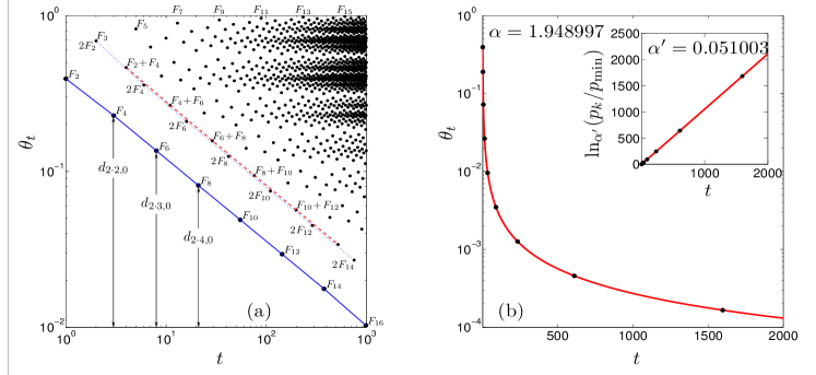
Figure 3: (a) Iteration time dependence of positions $\theta_{t}$ in logarithmic scales for the orbit with initial condition $\theta_{0}=0$ at $\Omega_{\infty}^{\prime}$ of the critical circle map $K=1$. The labels indicate iteration time $t$, the blue line goes through positions at times of the form $F_{2n}$, while the dotted and dashed lines do similarly at times of the form $2F_{2n}$ and $F_{2n}+F_{2n-2}$, respectively. The arrows indicate the distances equivalent to the principal diameters $d_{2n,0}$. (b) The positions $\theta_{t}$ of the trajectory in (a) at selected iteration times $t=F_{2n}-1$ (black dots) reproduced by Eq. (17) with $\alpha=1.948997$ (red). The inset shows the same data plotted in $\ln_{\alpha^{\prime}}$ scale, $p_{k}=1/\theta_{k}$, $p_{\min}=1$ and $\alpha^{\prime}=0.051003$. The straight line evidences the (time) extensivity of the entropy in Eq. (13). See text for description.

5 Phase space contraction and maximum entropy

As we have seen in the previous sections the contraction of phase space guided by the attractors at the three types of transitions to chaos is described quantitatively by the time evolution of trajectory positions. The expressions for these trajectory positions are conveniently obtained from the RG fixed-point maps at the transitions to chaos, and in all cases are exactly given by $q$-exponential functions. See Eqs. (10), (14) and (17). These functions replace the ordinary Boltzmann weights in generalized statistical-mechanical expressions associated with entropies of the Tsallis type that are written in terms of the inverse function, the $q$-logarithm. See Eqs. (1) and (2). We show now that these expressions can be obtained also from a Maximum Entropy Principle (MEP) and discuss further the occurrence of the dual indexes $\alpha$ and $\alpha^{\prime}=2-\alpha<1$ in relation to phase-space contraction.

Consider the entropy functional $\Phi_{1}[p_{k}]$ of the probabilities $p_{k}$, $k=0,1,2,\ldots,k_{\max}$ with Lagrange multipliers $a$ and $b$,

$$\Phi_{1}[p_{k}]=S_{1}[p_{k}]+a\left[\sum_{k=0}^{k_{\max}}p_{k}-\mathcal{P}\right]+b\left[\sum_{k=0}^{k_{\max}}kp_{k}-\mathcal{K}\right],$$ (18)

where the entropy expression $S_{1}[p_{k}]$ has the trace form

$$S_{1}[p_{k}]=\sum_{k=0}^{k_{\max}}s_{1}(p_{k}).$$ (19)

Optimization via $\partial\Phi_{1}[p_{k}]/\partial p_{k}=0$, $k=0,1,2,\ldots,k_{\max}$, gives $s_{1}^{\prime}(p_{k})=-a-bk$. Now, the choices $s^{\prime}_{1}(p_{k})=\ln_{\alpha}p_{k}^{-1}-p_{\min}^{-(1-\alpha)}+(1-\alpha)\mathcal{N}^{-1}k$, $a=-\ln_{\alpha}p_{\min}^{-1}+p_{\min}^{-(1-\alpha)}$, $b=\alpha\mathcal{N}^{-1}$, lead to

$$\ln_{\alpha}\ p_{k}^{-1}=\ln_{\alpha}p_{\min}^{-1}-\mathcal{N}^{-1}k.$$ (20)

or

$$p_{k}^{-1}=p_{\min}^{-1}\exp_{\alpha}(-p_{\min}^{1-\alpha}\mathcal{N}^{-1}k).$$ (21)

from which we immediately recover Eq. (11). But also, importantly, $S_{1}[p_{k}]$ in Eq (19) becomes Eq. (1).

Consider next the same functional as above but with the probabilities $p_{k}$ replaced now by the new set $\pi_{k}$, $k=0,1,2,\ldots,k_{\max}$. We write

$$\Phi_{2}[\pi_{k}]=S_{2}[\pi_{k}]+c\left[\sum_{k=0}^{k_{\max}}\pi_{k}-\mathcal{P}^{\prime}\right]+d\left[\sum_{k=0}^{k_{\max}}k\pi_{k}-\mathcal{K}^{\prime}\right].$$ (22)

So that $s^{\prime}_{2}(\pi_{k})=-c-dk$, with the choices $s^{\prime}_{2}(\pi_{k})=-\ln_{\alpha^{\prime}}\pi_{k}-\pi_{\min}^{1-{\alpha^{\prime}}}-(1-{\alpha^{\prime}})\mathcal{N}^{-1}k$, $c=\pi_{\min}^{1-{\alpha^{\prime}}}+\ln_{\alpha^{\prime}}\pi_{\min}$, $d=(2-\alpha^{\prime})\mathcal{N}^{-1}$, lead to

$$\ln_{\alpha^{\prime}}\ \pi_{k}=\ln_{\alpha^{\prime}}\pi_{\min}+\mathcal{N}^{-1}k.$$ (23)

or

$$\pi_{k}=\pi_{\min}\exp_{\alpha^{\prime}}(\pi_{\min}^{\alpha^{\prime}-1}\mathcal{N}^{-1}k),$$ (24)

which, also importantly, when used to evaluate $S_{2}[\pi_{k}]$ leads to Eq. (2).

If the probabilities $p_{k}$ and $\pi_{k}$ correspond, respectively, to the initial and the contracted sets of configurations, and if they are both normalizable in their own spaces, then to recover one from the other we require a relationship such as

$$\pi_{k}=p_{k}^{\alpha^{\prime}},$$ (25)

with $\alpha^{\prime}<1$ when the contracted set has a vanishing measure with respect to the initial one. Therefore we note that in the MEP procedure it is not necessary to make use of the constraint

$$\sum_{k=0}^{k_{\max}}k\ p_{k}^{\alpha^{\prime}}=\textnormal{constant},$$ (26)

commonly used in the derivation of generalized entropies [6], including Ref. [14] (where there appears some non-consequential faux pas). Instead, the distinction between the initial and contracted space of configurations indicates the introduction of a contraction dimension $\alpha^{\prime}$ via Eqs. (3) or (25).

6 Discussion

We have discussed the association of dual entropy expressions of the Tsallis type with the dynamical properties of attractors in low-dimensional iterated maps along the three routes to chaos: intermittency, period doublings and quasi-periodicity. The attractors at the transitions to chaos provide a natural mechanism by means of which ensembles of trajectories are forced out of almost all phase space positions and become confined into a finite or (multi)fractal set of permissible positions. Such drastic contraction of phase space leads to nonergodic and nonmixing dynamics that is described by the dual entropic indexes $\alpha>1$ and $\alpha^{\prime}=2-\alpha<1$. The first fixes the deformation of the exponential that measures the degree of contraction along (iteration) time evolution, and the second defines a contraction dimension, cf. Eq. (3), such that extensivity of entropy is restored. The dual entropy expressions are compatible with the same maximum entropy principle. When the contraction of phase space leads to a set of configurations of the same measure as the original phase space, e.g., an interval or finite collection of intervals of real numbers, one has $\alpha=\alpha^{\prime}=1$, the entropy expressions are the same and maintain the usual BG expression.

We chose to examine the statistical-mechanical effect of configuration space contraction at the renowned transitions to chaos in low-dimensional nonlinear maps, as these are perhaps the simplest situations where ergodicity and mixing properties breakdown. But in their own, the properties of these model systems manifest in natural phenomena. There are abundant examples of ranked data that obey (approximately) the empirical Zipf power law and these have been shown to comply with the tangent bifurcation property [14]. The period doubling cascade to chaos has been considered recently in many model systems ranging from fluid convection [17] to urbanization processes [18]. The basic features of the quasi periodic route to chaos have been famously measured in forced Rayleigh-Benard convection [19] and in periodically perturbed cardiac cells [20].

7 Acknowledgements

The authors are grateful for the interest of Murray Gell-Mann in this work, and for his valuable advice and recommendations. G.C.Y. gratefully acknowledges the hospitality of the Santa Fe Institute. G.C.Y. was supported by the Scientific Research Projects Coordination Unit of Istanbul University with project number 49338. A.R. acknowledges support by DGAPA-UNAM-IN103814 and CONACyT-CB-2011-167978 (Mexican Agencies).

References

- [1] J. Uffink, “Compendium to the foundations of classical statistical physics,” in Handbook for the Philosophy of Physics (J. Butterfield and J. Earman, eds.), pp. 924–1074, Elsevier, Amsterdam, 2007.
- [2] P. G. De Benedetti and F. H. Stillinger, “Supercooled liquids and the glass transition,” Nature, vol. 410, no. 6825, pp. 259–267, 2001.
- [3] H. G. Schuster, Deterministic Chaos. An Introduction. VCH Publishers, Weinheim, 1988.
- [4] C. Beck and F. Schlogl, Thermodynamics of Chaotic Systems. Cambridge University Press, Cambridge, 1993.
- [5] A. Robledo, “Generalized statistical mechanics at the onset of chaos,” Entropy, vol. 15, no. 12, pp. 5178–5222, 2013.
- [6] C. Tsallis, Introduction to Nonextensive Statistical Mechanics: Approaching a Complex World. Springer, New York, 2009.
- [7] F. Baldovin and A. Robledo, “Sensitivity to initial conditions at bifurcations in one-dimensional nonlinear maps: Rigorous nonextensive solutions,” Europhys. Lett., vol. 60, no. 4, pp. 518–524, 2002.
- [8] M. Mayoral and A. Robledo, “Tsallis index and Moris phase transitions at the edge of chaos,” Phys. Rev. E, vol. 72, no. 2, pp. 026209–1–7, 2005.
- [9] H. Hernández-Saldaña and A. Robledo, “Fluctuating dynamics at the quasiperiodic onset of chaos, Tsallis -statistics and Moris -phase thermodynamics,” Physica A, vol. 370, no. 2, pp. 286–300, 2006.
- [10] C. Altamirano and A. Robledo, “Possible thermodynamic structure underlying the laws of Zipf and Benford,” Eur. Phys. J. B, vol. 81, no. 3, pp. 345–351, 2011.
- [11] A. Robledo, “Laws of Zipf and Benford, intermittency, and critical fluctuations,” Chinese Sci. Bull., vol. 56, no. 34, pp. 3645–3648, 2011.
- [12] L. Pietronero, E. Tosatti, V. Tosatti, and A. Vespignani, “Explaining the uneven distribution of numbers in nature: the laws of Benford and Zipf,” Physica A, vol. 293, no. 1-2, pp. 297–304, 2001.
-
[13]
Website of the Santa Fe Institute,
http://www.santafe.edu/about/people/profile/AaronClauset;
Aaron Clauset home page Data and Code,
http://tuvalu.santafe.edu/ãaronc/powerlaws/data.htm, accessed August 29, 2015. - [14] G. C. Yalcin, A. Robledo, and M. Gell-Mann, “Incidence of statistics in rank distributions,” Proc. Natl. Acad. Sci. USA, vol. 111, no. 39, pp. 14082–14087, 2014.
- [15] A. Robledo and L. G. Moyano, “-deformed statistical-mechanical property in the dynamics of trajectories in route to the Feigenbaum attractor,” Phys. Rev. E, vol. 77, no. 3, pp. 036213–1–14, 2008.
- [16] A. Diaz-Ruelas and A. Robledo, “Emergent statistical-mechanical structure in the dynamics along the period-doubling route to chaos,” Europhys. Lett., vol. 105, no. 4, pp. 40004–1–6, 2014.
- [17] H. Yahata, “Period-doubling cascade to chaos of the Rayleigh-Benard convection in a rectangular box,” J. Phys. Soc. Jpn, vol. 83, no. 11, pp. 114401–1–7, 2014.
- [18] Y. Chen and F. Xu, “Modeling complex spatial dynamics of two-population interaction in urbanization process,” Journal of Geography and Geology, vol. 2, no. 1, pp. 1–17, 2010.
- [19] J. A. Glazier and A. Libchaber, “Quasi-periodicity and dynamical systems: An experimentalists view,” IEEE Transactions on Circuits and Systems, vol. 35, no. 7, pp. 790–809, 1988.
- [20] M. R. Guevara, L. Glass, and A. Shrier, “Phase locking, period-doubling bifurcations, and irregular dynamics in periodically stimulated cardiac cells,” Science, vol. 214, no. 4527, pp. 1350–1353, 1981.