Quasinormal modes of Gauss-Bonnet black holes
at large
Bin Chena,b,c111bchen01@pku.edu.cn, Zhong-Ying Fanc222fanzhy@pku.edu.cn, Pengcheng Lia333wlpch@pku.edu.cn, Weicheng Yea444victorye@pku.edu.cn
aDepartment of Physics and State Key Laboratory of Nuclear Physics and Technology,
Peking University, No.5 Yiheyuan Rd, Beijing 100871, P.R. China
bCollaborative Innovation Center of Quantum Matter, No. 5 Yiheyuan Rd,
Beijing 100871, P. R. China
cCenter for High Energy Physics, Peking University, No.5 Yiheyuan Rd,
Beijing 100871, P. R. China
Abstract
Einstein’s General Relativity theory simplifies dramatically in the limit that the spacetime dimension is very large. This could still be true in the gravity theory with higher derivative terms. In this paper, as the first step to study the gravity with a Gauss-Bonnet(GB) term, we compute the quasi-normal modes of the spherically symmetric GB black hole in the large limit. When the GB parameter is small, we find that the non-decoupling modes are the same as the Schwarzschild case and the decoupled modes are slightly modified by the GB term. However, when the GB parameter is large, we find some novel features. We notice that there are another set of non-decoupling modes due to the appearance of a new plateau in the effective radial potential. Moreover, the effective radial potential for the decoupled vector-type and scalar-type modes becomes more complicated. Nevertheless we manage to compute the frequencies of the these decoupled modes analytically. When the GB parameter is neither very large nor very small, though analytic computation is not possible, the problem is much simplified in the large expansion and could be numerically treated. We study numerically the vector-type quasinormal modes in this case.
1 Introduction
In Einstein’s General Relativity, the vacuum equation takes a very simple form
| (1.1) |
However mathematically concise and beautiful it looks, the equation is a set of coupled highly non-linear partial differential equations. The nonlinearity makes it extremely difficult to analyze. In recent years, Emparan, Suzuki and Tanabe (EST) [1, 2, 3] proposed an ingenious method called “Large Expansion” to study the dynamics of the black holes. EST considers the limit that the spacetime dimension is very large and develops a systematic way to do expansion. This method was inspired by the large expansion of gauge theories[4, 5]. Extended objects called strings are formulated in the large expansion of Yang-Mills theories and the counterpart of the string in the Large expansion of gravity is the black hole. A Schwarzschild black hole of a Schwarzschild radius in spacetime dimensions is described by the metric [6]
| (1.2) |
We can see that the geometry of a black hole in spacetime dimensions is non-trivial only in a distance away from its event horizon outside of which the geometry can be essentially taken as the Minkowskian spacetime. Therefore, the black holes can be regarded as non-interacting “particles” of finite radius but vanishingly small cross sections [1]. Thus, the focus of EST’s work has been mainly on these non-perturbative extended objects, while the black branes and the membranes have also been considered in their work and the following works by other groups555For another large D limit, see [12]. [1, 2, 3, 7, 8, 9, 10, 11].
Most importantly, EST have developed a systematic method of computing the quasinormal modes by the expansion and obtained the results in perfect agreement with previous numerical results [7, 9, 10]. They found that there are two kinds of quasinormal modes, the non-decoupling ones and the decoupled ones. The non-decoupling ones are non-renormalizable in the near horizon geometry, and such modes have frequencies of order . These modes, however, are universally shared among all spherically static black holes since they essentially reflect the asymptotic flatness of the black hole so that they carry little information about the black hole geometry. Besides, there are decoupled modes localized within the near horizon region, with their frequencies being of order . In contrast to the non-decoupling modes, the decoupled modes is tightly related to the specific black hole geometry beyond the leading large limit. Therefore, their values at the higher orders exhibit detailed near-horizon properties of a specific black hole.
The quantum corrections to the classical general relativity implies the existence of the higher curvature terms. Among the higher curvature terms, the so-called Gauss-Bonnet(GB) term is of particular interest. It is made up of the quadratic terms in curvature, and appears as the leading correction in string theory[13, 14]. This term is a simple topological term when , and becomes physically relevant only when . Including the Gauss-Bonnet term into the gravity action, we get
| (1.3) |
where is a parameter for the GB term. This action describes the so-called Einstein-Gauss-Bonnet gravity or simply Gauss-Bonnet gravity. One nice thing about this action is that the equation of motion is still of second order and there is no ghost. Another nice thing is that there are well-known black hole solutions in this theory.
A natural generalization of EST’s work is to perform a large expansion in the Gauss-Bonnet gravity theory. As the first step, we would like to compute the quasi-normal modes of a spherically symmetric GB black hole in the large expansions. The master equations for the scalar-, vector- and tensor-type perturbations have been computed in [15, 16, 17, 18]. A complete numerical analysis of the evolution of the gravitational perturbations for -dimensional Gauss-Bonnet black holes with was performed by Konoplya [18], and the stability and instability regions have been determined comprehensively there. The aim of our work is to perform a systematic calculation of quasinormal modes in the large expansion.
The Gauss-Bonnet term could be originated from the string theory which might restrict the value of the parameter . However, in this work, we just focus on the Gauss-Bonnet gravity, without restricting the value of . In the large expansion, the value of the parameter determines the contribution of the GB term. It is easy to see that the Riemann tensor scales as , and therefore the Einstein term also scales as while the Gauss-Bonnet term scales as ! It is natural to assume that the value of does not change with , leading to a theory that is dominant by the Gauss-Bonnet term at large . Under such circumstance the magnitude of the Einstein term is of two less orders than that of the Gauss-Bonnet term, and we can regard the theory as a “pure” Gauss-Bonnet theory at large which includes only the Gauss-Bonnet term, plus a small perturbation. The situation when or larger is similar and we can just take as an illustrative example. On the other hand, when scales as or less, the Einstein term dominates, and the black hole can be regarded as an Einstein black hole with small perturbations from the Gauss-Bonnet term. Analytical results can be obtained for both the small and large cases. The situation becomes complicated if scales as . In this case the magnitude of the Einstein term is the same as that of the Gauss-Bonnet term. Although in the large expansion the problem can still be simplified dramatically, the analytical treatment is not feasible and the numerical calculations have to be carried out.
The paper is organized as follows. In Sec. 2 we introduce the geometry of the Einstein-Gauss-Bonnet black hole in the large expansion. In Sec. 3 we discuss briefly the quasinormal modes for a minimally-coupled scalar field. In Sec. 4 and Sec. 5 we study the non-decoupling and decoupled quasinormal modes respectively. In Appendix, we give numerical results for the decoupled vector-type quasinormal modes of “hybrid” Gauss-Bonnet black holes at the leading order.
2 Basic geometry
The metric of a spherically symmetric and static black hole in the Einstein-Gauss-Bonnet gravity could be written as[14]
| (2.1) |
| (2.2) |
where is the mass of the black hole. The horizon is at which is related to the mass by the relation
| (2.3) |
For convenience we can set and introduce an useful quantity
| (2.4) |
In terms of the and can be expressed as
| (2.5) |
In order to discuss the large expansion, we introduce an expansion parameters
| (2.6) |
and let
| (2.7) |
2.1 Small
When is small, for example , the second term in is very small so can be expanded as a power-series of . This is always possible because we are interested in the geometry outside the horizon such that and therefore . In order to precisely represent the “smallness” of , we introduce a new parameter , which is of order one . Using expansion the above formulas can be expanded as
| (2.8) |
| (2.9) |
In this case the near region is , or and the far region is . Obviously, when we recover the Schwarzschild case in pure Einstein gravity.
We could expect that in the case that is small, the corrections originating from the Gauss-Bonnet term must be small. From the expansion in the function , the effects from the Gauss-Bonnet term should only be reflected at the order or even higher order terms. In the limit we should reproduce the results in the Schwartzschild black hole in the Einstein gravity.
2.2 Large
When is large enough, for example and , in the region where , the second term in dominates and we could expand it in series of , so the forms of and are expanded as
| (2.10) |
| (2.11) |
The validity of the expansion requires that , which we will refer to as the near region although it is smaller than the usual near region where . This is all right since it still has overlap with the far region .
When is a little smaller, e.g. or even larger e.g., the discussion on the expansion is similar. The only difference is that the near region becomes smaller or larger . Therefore we will treat as a typical example for the large case and discuss it explicitly.
However, when takes an intermediate value, i.e. , even in the large expansion the metric is too complicated for us to compute the quasinormal modes analytically. In this case, the leading order form of is given by
| (2.12) |
which is quite different from (2.9) or (2.11). As a result there are different spectrums for the decoupled modes which are not universal and depend on the specific black hole geometry. In the appendix we present the numerical result of vector-type quasinormal modes at leading order to show this point.
3 The quasinormal modes for a scalar field
As the first step, let us consider a minimally-coupled scalar in the black hole background. As the black hole geometry is spherically symmetric, the scalar wavefunction could be decomposed into the following form
| (3.1) |
where is the frequency and is the spherical harmonic function. The differential equation for the radial function is
| (3.2) |
where , , . The above equation can be recast into a master equation of the form
| (3.3) |
where
| (3.4) |
| (3.5) |
The height of the potential is . Since the potential varies slowly in the overlapping zone, we can treat it as a constant. As a consequence, the differential equation (3.3) in the overlapping region takes the form
| (3.6) |
In fact this form of the radial equation is independent of the value of , although the range of the overlapping region depends on . If , the solution of this equation is
| (3.7) |
while if , the solution is of the form
| (3.8) |
where , are integration constants.
The quasinormal modes are the solutions of (3.3), which should satisfy the ingoing boundary condition at the event horizon and the outgoing boundary condition at the infinity. At the horizon this requires
| (3.9) |
when is small and
| (3.10) |
when is large. Here is some regular function at .
The strategy to find the quasinormal modes is to solve the differential equation of the perturbation in the far region and the near region with appropriate boundary conditions. The matching of the solutions in the overlapping region then determines the quasinormal modes.
3.1 Near-region solutions
3.1.1 Small
For a small , consider the leading order in the expansion in the near region, from the behavior of in (2.9) we see that the differential equation (3.2) is exactly the same as the one in the Schwarzschild black hole, which is of a hypergeometric type. Hence the solution that satisfies the ingoing boundary condition at the horizon is exactly the same as the result in [1],
| (3.11) |
where
| (3.12) |
3.1.2 Large
For a large , up to the order, the radial equation is simplified to be
| (3.13) |
The solution is
| (3.14) |
where
| (3.15) |
The boundary condition (3.10) selects the solution to be
| (3.16) |
As discussed in [9], the only information that we need from the solution is their large behavior in the overlapping region where . It is easy to find that for a general no matter what value takes there is always
| (3.17) |
When , the solution should be in match with (3.8) in the overlapping region, leading to
| (3.18) |
3.2 Far-region solutions
In the far-region, is exponentially small. Thus we can set no matter what value takes and the radial equation (3.3) is exactly the same as the one in the Minkowski spacetime, so the solution is just the Hankel functions [9]
| (3.19) |
Following the discussion in [9], in the overlapping region, in terms of the coordinate the solution takes the form (3.7) or (3.8).
3.3 Quasinormal modes
As we have seen, the far-region solution is exactly the same as the one in the Schwarzschild black holes whatever takes. On the other hand in the near region, the radial equation for a small is identical to the scalar equation in the Schwarzschild black hole background. But for a large the radial equation and its solution in the near region is different. Nevertheless the useful information in the overlapping region is encoded in Eqs. (3.17) and (3.18), the same as the ones in the Schwarzschild case.
If we try to paste the solutions in all regions satisfying the appropriate boundary conditions, we see that even though the solution in the near region could be different, the solution in the overlapping region is the same as the Einstein gravity. Consequently we conclude that the quasinormal modes for a scalar field in the Gauss-Bonnet black hole (2.1) are completely the same as the ones in the Schwarzschild black hole background.
4 Non-decoupling modes for gravitational perturbations
In the last section, we discussed the quasinormal modes of a scalar field in the Gauss-Bonnet black hole background. The scalar field is taken as a probe and is minimally coupled to the gravity. It could only probe the geometry of the background but cannot see the dynamics of the Gauss-Bonnet gravity. In this section, we discuss the gravitational perturbation in the Gauss-Bonnet gravity. This may allow us to investigate the dynamics of the theory.
The linearized gravitational fluctuations could be classified according to their transformation properties under the rotation group: scalar-type(S), vector-type(V) and tensor-type(T) gravitational perturbations. Each type of the perturbations satisfies the master equation of the form
| (4.1) |
where denotes three types of the perturbations. The potentials in (4.1) depend on the types of the perturbation [18]
| (4.2) |
| (4.3) |
| (4.4) |
and
| (4.5) |
| (4.6) |
| (4.7) |
| (4.8) |
The discussion on the non-decoupling quasinormal modes is similar to the one for the scalar field in the previous section. In order to find the quasinormal modes, one need to solve the master equation in two different regions and then match them in the overlapping region.
4.1 Small
Up to the leading order in , the metric is the same as the one in the Schwarzschild case, so we could expect that the quasinormal modes are the same as long as we only keep to leading order. Although the three potential forms are complicated, the GB effect appears only at the next-to-leading order. Actually the leading order form of the three potentials are
| (4.9) |
| (4.10) |
| (4.11) |
All of them are independent of so that the GB term has no effect on the non-decoupling quasinormal modes in the small case.
4.2 Large
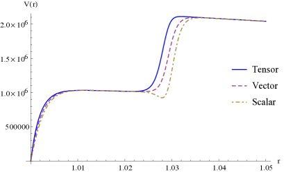
In Fig. 1, we show the potentials for different types of gravitational perturbation in the very large limit. Here we choose , , and . From Fig. 1, we find that there are two plateaux, a fact that is very different from the Schwarzschild case. The lower one is unique for the Einstein-Gauss-Bonnet gravity and it disappears in the limit that goes to zero. Its height is . It is in the range of the near horizon region we defined before so that it is suitable for the expansion. The higher one is beyond the near horizon region, and its height is , the same as the one in the Schwarzschild case, since the Gauss-Bonnet black hole we considered is also asymptotically flat. Recall that the non-decoupling modes are non-normalizable in the near horizon geometry. The real part of the frequency of the non-decoupling quasinormal modes is lower than the maximum of the potential. As now there are two separated plateaux in the potential, there might be two different sets of non-decoupling modes. Let us work them out in detail.
4.2.1 Lower plateau
Let us focus on the lower plateau first. Up to the leading order in the expansion the heights of the three potentials are the same, so in this case the basic form of the solutions of the master equation (4.1) in the overlapping region must be
| (4.12) |
where we have defined a new quantity . When there is
| (4.13) |
For different types of the perturbations, the potentials in the master equation take different forms. Up to the leading order they are respectively
| (4.14) |
| (4.15) |
| (4.16) |
For the tensor- and vector-perturbations, their equations are of hypergeometric types. Taking into account the boundary condition at the horizon the solutions are respectively
| (4.17) |
| (4.18) |
where
| (4.19) |
For the scalar-type potential the equation is more complicated. As in the case discussed in [9], the scalar solution can be expressed as some differential operators acting on a hypergeometric function.
The only information that we need from the solutions is their large behaviors in the overlapping region where . It is easy to find that for general , we have
| (4.20) |
while for ,
| (4.21) |
Similarly in the far-region we may set , and the outgoing solution is the Hankel function
| (4.22) |
In terms of the coordinate the solution can take the form (4.12) or (4.13).
The matching of the near- and far-region solutions give the non-decoupling modes whose frequency are of order . As discussed in [9], the least-damped modes have analytic expressions and the case of higher overtones could be described numerically. Here, we present the real part and the imaginary part of the least-damped mode frequencies as follows
| (4.23) |
and
| (4.24) |
where correspond to the zeros of the Airy function.
4.2.2 Higher plateau
On the other hand, the higher plateau should also generate the non-decoupling quasinormal modes. The solution should have such that the wave is purely outgoing with no reflection in the overlapping region, but gets reflected in the far region due to the presence of the second plateau. Because the second plateau is in the far-region the usual far-region solution (4.22) still works, and the non-decoupling modes are determined by the far-region solutions. Although the plateau is beyond the near-region, through a variable replacement we can pull it back to the near region. For example, after the replacement the leading order tensor potential becomes
| (4.25) |
In the limit that , as we expected. Near the edge of the second plateau , this corresponds so the solution should be connected with far-region solution of . We will not illustrate this point in detail since the most important information is the amplitude ratios in front of wave-function components. The far-region solution tells us that in the case of the quasinormal modes should be identical to the ones in the Schwarzschild case, so for the least-damped modes the frequency spectrum is
| (4.26) |
and
| (4.27) |
As a conclusion we find that the interesting things happen when the GB coupling is very large. There are two kinds of non-decoupling quasinormal modes, one kind is the same as the one in the Schwarzschild black holes. This kind of modes is universal for all asymptotically flat static black holes. The other kind is special for the GB black holes due to the emergence of a new plateau in the potential when is large enough.
5 Decoupled modes for gravitational perturbations
The decoupled modes are normalizable in the near horizon geometry. They are localized within the near horizon region and decoupled with the asymptotically flat region. Their frequencies are of order one. To leading order in , these modes are static and becomes dynamical at the next-to-leading order. They can be studied in the expansion order by order.
The form of the master equation can be recast into the form
| (5.1) |
where
| (5.2) |
| (5.3) |
All quantities can be expanded in powers of as
| (5.4) |
such that the decoupled modes can be studied perturbatively.
The equation for the perturbation at each order is determined by the differential equation with a source
| (5.5) |
Here the sources are obtained from with , and from the solutions with .
At each order, the solution should be normalizable. The strategy to read the decoupled modes is to first compute the lowest order solution and then compute the higher order solution order by order.
5.1 Small
In this case, to the leading order
| (5.6) |
The equation is exactly the same as the Schwarzschild case, and the Gauss-Bonnet effect is absent. At the next-to-leading order there are corrections from the Gauss-Bonnet term
| (5.7) |
As the decoupled modes are normalizable, the boundary condition at is
| (5.8) |
This is because the maximum of all the three potentials is , with , in the overlapping region, where . The master equation now has the form
| (5.9) |
For the decoupled modes , the normalizability of the solution requires . The other solution being proportional to is non-normalizable and is excluded.
The boundary condition at the event horizon is required by its regularity. This asks the solution to be
| (5.10) |
where is the tortoise coordinate. Expanding in series of , the explicit forms at each order are respectively
| (5.11) | |||||
| (5.12) | |||||
| (5.13) | |||||
| (5.14) | |||||
etc. Note that there are corrections from the GB term in .
5.1.1 Tensor type
For the tensor-type perturbation, the leading order potential is
| (5.15) |
which is the same as the Schwarzschild black hole. The solutions are
| (5.16) |
Obviously, neither of the two solutions can satisfy the two boundary conditions simultaneously, so there is no decoupled quasinormal mode of the tensor type.
5.1.2 Vector type
The vector potential at the leading order is given by
| (5.17) |
The two independent solutions are
| (5.18) |
The two boundary conditions determine that
| (5.19) |
At the next-to-leading order, the potential is given by
| (5.20) |
The solution that satisfies the boundary condition at the infinity is
| (5.21) |
where is an integral constant. The boundary condition at the horizon requires and determines the frequency of the decoupled mode to be
| (5.22) |
Therefore at the next-to-leading order even though the vector potential is modified by the Gauss-Bonnet term, the quasinormal modes are the same as the ones in the Schwarzschild case.
At the order in , there are decoupled modes with the frequencies
| (5.23) |
Now, there is a correction from the Gauss-Bonnet term. This conforms to the expansion form of when is small. At the order in , the calculation is straightforward and leads to
| (5.24) |
5.1.3 Scalar type
Like the situation of the Schwarzschild black hole, in order to properly deal with the region where we need to introduce a new variable
| (5.25) |
Then the potential to the leading order becomes
| (5.26) |
This potential correctly captures all the features of the scalar potential in the near-region. Especially, in the region , we have a small which should be matched with the solution of for .
First of all it is straightforward to find the solutions for with the ingoing boundary condition at the horizon
| (5.27) |
| (5.28) |
Up to the second order, at the large the expansion of gives
| (5.29) |
To the second order, the solution for with the boundary condition as is
The match of two solutions at the leading order requires with being undetermined, but this is not sufficient to determine the frequency of the decoupled mode because there is term coming from . Indeed there is such a term
| (5.30) |
which, by matching with (5.29), determines that
| (5.31) |
This is equal to the result of the Schwarzschild black hole. One can proceed to find the frequency of the decoupled mode in the order
| (5.32) |
which encodes the correction from the Gauss-Bonnet term. The discussion for the higher order decoupled modes is similar and straightforward but becomes more and more complicated.
5.2 Large
In this case, there is
| (5.33) |
As in the situation of small , the boundary condition at the horizon can be given order by order as
| (5.34) | |||||
| (5.35) | |||||
| (5.36) | |||||
| (5.37) | |||||
etc. The boundary condition at requires
| (5.38) |
Note that this is different from the Schwarzschild case, because the maximum of all the three potentials in the large case is . In order to be normalizable, the decoupled modes should satisfy (5.38).
5.2.1 Tensor type
The leading order of the tensor potential is
| (5.39) |
and the corresponding solutions are
| (5.40) |
Obviously, none of the two solutions can satisfy the two boundary conditions simultaneously, and there is no decoupled quasinormal modes of tensor type.
5.2.2 Vector type
The leading order of the vector potential is given by
| (5.41) |
and the two independent solutions are
| (5.42) |
The boundary conditions select
| (5.43) |
so there could exist the quasinormal modes of vector type. At the next-to-leading order,
| (5.44) |
then the solution is
| (5.45) |
where and are two integration constants. The boundary condition at the infinity requires , and the boundary condition at the horizon determines the frequency to be
| (5.46) |
It is a surprise that this is exactly the same as the one in the Schwarzschild case found in [9]. At the second order in , the potential is
| (5.47) |
Then the solution can be easily obtained. With the help of the boundary condition at the horizon, the second order frequency can be read
| (5.48) |
which is different with the one in the Schwarzschild case due to different effect from the boundary conditions. Actually, there is instead of a simple from the ingoing boundary condition, and the quasinormal mode at the second order is accordingly changed. At the third order, it is straightforward to read
| (5.49) |
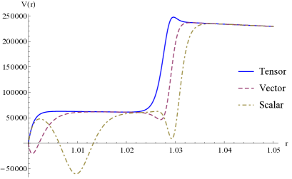
From Fig. 2 we see that the vector potential has two minima, the negative one on the left side and the positive one on the right side. The negative one gives the above decoupled mode. The positive one is new, which does not appear when is small, and its location is at . We would like to investigate whether the positive one gives new decoupled modes or it leads to the same wave function discussed above propagating through the whole regions. In order to properly deal with the region with positive minimum, we introduce a new variable
| (5.50) |
Since in the positive minimum region, we can study the wave function around the minimum using the expansion. The leading order vector potential in terms of is
| (5.51) |
In the limit that is very small the potential reaches which can be matched to the maximum of the potential (5.41) in the region . And when is very large the potential has a maximum which is the same as the Schwarzschild black hole, since the spacetime is asymptotically flat.
At the leading order the differential equation becomes
| (5.52) |
and its solutions are
| (5.53) |
At the large , gives the correct asymptotic behavior which is . At the small , scales as , this can be matched to the solution in the region .
Next let us extend the discussion to the next-to-leading order. The solution with the ingoing boundary condition at the horizon is
| (5.54) | |||||
Its large behavior is
| (5.55) |
On the other hand, to the same order the solution for with the correct boundary condition at the large is
| (5.56) | |||||
where is an integral constant. Then we make a replacement and expand the expression in . From the matching with (5.55) at the leading order, we can fix . To the next-to-leading order we get
| (5.57) |
The matching with (5.55) can determine all the undetermined constants ( term comes from the next order), among which we have
| (5.58) |
Hence this verifies that the positive minimum do not give any new decoupled mode. Actually, the wave in the left valley of the potential propagate right to the next valley. In other words, once we find the solution in the left valley, we can extend it to the right and using the matching condition in the overlapping region we can determine the wavefunction in the right valley completely.
It seems that the decoupled modes are only determined by the wavefunction in the left potential valley with the asyptotically boundary condition . This is due to the fact that the potential plateau between two minima has a long enough extension. As we discussed above, the wavefunction in the second valley could be determined by the matching of the solution. A better treatment is to find the solutions in different regions and paste them correctly, and then read the frequency of the decoupled modes. We will have to use this treatment for the scalar type perturbation in the next subsection.
5.2.3 Scalar type
We follow the similar treatment in the small case. However now the first minimum locates at , so the correct variable should be
| (5.59) |
then the scalar potential in the leading order becomes
| (5.60) |
From this expression we can read all the features appearing in Fig. 2: it reaches the same maxima at the small and the large , and reaches a minimum between these two maxima at . Note that the scalar potential has a local maximum before the minimum.
To determine the decoupled modes, we need to find the solutions in different regions and paste them correctly. First let us first match the solutions for and the solutions for in the region . It is easy to find the solutions for . With the ingoing boundary condition at the horizon, we get
| (5.61) |
| (5.62) |
In the large region, becomes
| (5.63) | |||||
On the other hand, up to the next-to-leading order the solution for with the boundary condition is
Comparing with (5.63), we find that the matching at the leading order requires that as before and the term is given at the next order in . However, a little subtlety here is that the third order wavefunction is not convergent any more for large , and it seems that the far region boundary condition cannot be achieved. However, there is nothing bad that truly happens. This can be explained by examining Fig. 2 carefully. The figure shows clearly that the scalar potential is very different from the vector and the tensor potentials with a remarkable feature that the plateau connecting the two valleys may not be sufficient long and high for the wavefunction to decay into zero. Therefore the true far-region is in the higher plateau which has the same structure as the Schwarzschild black holes. For the first and the second order wave functions the lower plateau is long enough so that they would not stretch into the higher plateau, but for the third and higher order wave functions the wave stretches into farther region. Therefore we need to discuss the wavefunction in the second valley carefully.
To investigate the wave in the second valley, we introduce the variable
| (5.65) |
It can be used to investigate the region which is the location of the second valley and the edge of the higher plateau. The leading order potential is now
| (5.66) |
In the limit , which is the height of the middle plateau. Moreover when , gives the correct far-region behavior of GB black holes. The wave functions should satisfy the boundary condition
| (5.67) |
With the potential and the boundary condition, the leading order solution is
| (5.68) |
On the other hand, at a small we find so that it can be matched to the solution .
Therefore we have three pieces of wave functions: the first is which satisfies the ingoing boundary condition at the event horizon, the second is which is valid in the first valley in Fig. 2 and matches with in the region , the third is which is valid in the second valley and satisfies the far-region boundary condition (5.67) and can be matched with in the region . The three pieces should be matched in the overlapping region, which constrains all of the undetermined constants in solving the differential equation. This computation can be carried out order by order. At the first order all the boundary conditions can be satisfied provided that we have
| (5.69) |
At the next order, the frequency is
| (5.70) |
Similar to the vector-type decoupled modes, the scalar decoupled mode at the first order is the same as the one in the Schwarzschild case, but the scalar mode at the second order is different.
6 Summary and discussions
In this paper we studied the quasinormal modes of the Gauss-Bonnet black holes in the large D. We have obtained the quasinormal spectrum of a minimally coupled scalar field in the background of the Gauss-Bonnet black hole and three types of quasinormal modes of gravitational perturbations. Since the metric expansion depends on the value of the GB parameter , we chose two typical values, a small of order and a large of order to investigate. In the large D limit, the geometry of the Gauss-Bonnet black hole is qualitatively similar to the one of the Schwarzschild case: the near horizon region becomes very short and approach flat spacetime very quickly.
For the scalar field the quasinormal modes are identical to the ones in the Schwarzschild case[9], and they are independent of the coupling constant . This is in accord with the fact that the scalar quasinormal modes are universal and is insensitive to the black hole geometry.
When the effective GB parameter is small, the non-decoupling modes of the gravitational perturbations are identical to the ones in the Einstein gravity. This is easy to understand as the effect of the GB term is negligible. However, when the effective GB parameter is large, there is another set of decoupling quasinormal modes, besides the ones in the Schwarzschild case. This is due to the appearance of another plateau in the radial potential. The basic picture is that even if the GB black hole and Schwarzschild black holes share the same asymptotic geometry, the near region geometry is slightly different so that the non-decoupling modes in two cases are slightly different. Nevertheless, all the non-decoupling modes are non-renormalizable in the near horizon geometry, and their frequencies .
For the decoupled modes, when the parameter is small, the effect of the Gauss-Bonnet term only appears beyond the leading order. This is within our expectation since the Gauss-Bonnet term is just a small modification to the Einstein’s gravity after all. When the parameter is large, the radial potentials for the vector-type and scalar type present new features: there are two minima rather than one, and the shapes of the potentials for the vector and the scalar are different. There are a few remarkable points:
-
1.
There is no tensor-type decoupled mode. This can be seen easily from the potential: there is no place to define a normalizable mode.
-
2.
For the vector-type perturbation, one can read the decoupled modes from the wavefunction in the first valley, as the plateau between two valleys are long enough.
-
3.
For the scalar-type perturbation, one has to compute the wavefunction in three regions and paste them correctly to read the decoupled modes.
-
4.
At the leading order the frequencies of the decoupled modes are the same as the ones in the small . This is a little surprise since in this case the Gauss-Bonnet term should be dominant, and it raises an issue if the leading decoupled mode is universal or not. However the numerical analysis of the vector-type modes in the appendix shows that this is just a coincidence and even at the leading order the frequencies are not universal when takes an intermediate value.
It would be interesting to compare our analytic results with the numerical study. In [18], the quasinormal modes of the GB black holes have been studied numerically in for a large . It was found that the instability in disappears in larger . To compare with our results obtained in this paper, one has to push the study to much larger .
The study of the quasi-normal modes in the Gauss-Bonnet black hole at a large D is the first step to understand the black hole dynamics in the Gauss-Bonnet gravity. The decoupled modes encodes the nontrivial black hole physics. It would be interesting to extend the study to the nonlinear regime, as suggested recently in [11, 19].
Acknowledgments
The work was in part supported by NSFC Grants No. 11275010, No. 11335012 and No. 11325522. BC would like to thank the participants of the advanced workshop “Dark Energy and Fundamental Theory” supported by the Special Fund for Theoretical Physics from the National Natural Science Foundations of China with Grant No. 11447613 for stimulating discussion.
Appendix A Numerical results of the first leading order of decoupled quasinormal modes of “hybrid” Gauss-Bonnet black holes
The computation of the decoupled modes in the Gauss-Bonnet black holes when is of order one is similar , but the analytical results are difficult to obtain. Therefore, one has to use numerical method to find the solution of ordinary differential equations with suitable boundary conditions. The large expansion can still simplify the numerical calculation dramatically. Here we list the decoupled quasinormal modes of the vector-type perturbations at the leading order in Table 1.
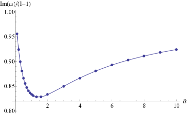
It is obvious that these decoupled quasinormal modes are all of the form , with varying between 0.8 to 1. The relation between and are plotted in Fig. 3, with a minimum at around . It indicates that black holes are more “stable” when the GB term or the Einstein term dominates. On the other hand, when the GB term and the Einstein term are comparable, the black holes are less “stable”.
References
- [1] R. Emparan, R. Suzuki, and K. Tanabe,The large limit of General Relativity, JHEP 1306 (2013) 009, [arXiv:1302.6382[hep-th]].
- [2] R. Emparan, D. Grumiller, and K. Tanabe, Large- gravity and low- strings, Phys.Rev.Lett. 110 (2013), no. 25 251102, [arXiv:1303.1995[hep-th]].
- [3] R. Emparan and K. Tanabe, Holographic superconductivity in the large expansion, JHEP 1401 (2014) 145, [arXiv:1312.1108[hep-th]].
- [4] G. ’t Hooft, A Planar Diagram Theory for Strong Interactions, Nucl.Phys. B72 (1974) 461.
- [5] E. Witten, Quarks, atoms, and the expansion, Physics Today 33 (1980).
- [6] F. R. Tangherlini, Schwarzschild field in dimensions and the dimensionality of space problem, Nuovo Cim. 27 (1963) 636.
- [7] R. Emparan and K. Tanabe, Universal quasinormal modes of large black holes, Phys.Rev. D89 (2014), no. 6 064028, [arXiv:1401.1957[hep-th]].
- [8] R. Emparan, R. Suzuki, and K. Tanabe, Instability of rotating black holes: large analysis, JHEP 1406 (2014) 106, [arXiv:1402.6215[hep-th]].
- [9] R. Emparan, R. Suzuki, and K. Tanabe, Decoupling and non-decoupling dynamics of large black holes, JHEP 1407 (2014) 113, [arXiv:1406.1258[hep-th]].
- [10] R. Emparan, R. Suzuki, and K. Tanabe, Quasinormal modes of (Anti-)de Sitter black holes in the expansion, JHEP 04 (2015) 085, [arXiv:1502.02820[hep-th]].
- [11] S. Bhattacharyya, A. De, S. Minwalla, R. Mohanc, and A. Saha, A membrane paradigm at large D, arXiv:1504.06613 [hep-th].
- [12] G. Giribet, “Large D limit of dimensionally continued gravity,” Phys. Rev. D 87, no. 10, 107504 (2013) doi:10.1103/PhysRevD.87.107504 [arXiv:1303.1982 [gr-qc]].
- [13] B. Zwiebach, Curvature Squared Terms and String Theories, Phys. Lett. B 156, 315 (1985).
- [14] D. G. Boulware and S. Deser, String-Generated Gravity Models, Phys. Rev. Lett. 55 (1985), no. 24 2656.
- [15] G. Dotti and R. J. Gleiser, Linear stability of Einstein-Gauss-Bonnet static spacetimes Part I: tensor perturbations, Phys. Rev. D72 (2005), no. 4, 044018, [arXiv:gr-qc/0503117].
- [16] R. J. Gleiser and G. Dotti, Linear stability of Einstein-Gauss-Bonnet static spacetimes- Part II: Vector and scalar perturbations, Phys. Rev. D72 (2005), no. 12, 124002, [arXiv:gr-qc/0510069].
- [17] R. G. Daghigh, G. Kunstatter and J. Ziprick, The Mystery of the Asymptotic Quasinormal Modes of Gauss-Bonnet Black Holes, Class. Quant. Grav. 24, 1981 (2007), [arXiv:gr-qc/0611139].
- [18] R. A. Konoplya and A. Zhidenko, (In)stability of -dimensional black holes in Gauss-Bonnet theory, Phys. Rev. D77 (2008), no. 10, 104004, [arXiv:0802.0267].
- [19] S. Bhattacharyya, M. Mandlik, S. Minwalla and S. Thakur, A Charged Membrane Paradigm at Large D, arXiv:1511.03432 [hep-th].