Quantum state transfer in optomechanical arrays

Abstract

Quantum state transfer between distant nodes is at the heart of quantum processing and quantum networking. Stimulated by this, we propose a scheme where one can highly achieve quantum state transfer between sites in a cavity quantum optomechanical network. There, each individual cell site is composed of a localized mechanical mode which interacts with a laser-driven cavity mode via radiation pressure, and photons exchange between neighboring sites is allowed. After the diagonalization of the Hamiltonian of each cell, we show that the system can be reduced to an effective Hamiltonian of two decoupled bosonic chains, and therefore we can apply the well-known results regarding quantum state transfer in conjuction with an additional condition on the transfer times. In fact, we show that our transfer protocol works for any arbitrary quantum state, a result that we will illustrate within the red sideband regime. Finally, in order to give a more realistic scenario we take into account the effects of independent thermal reservoirs for each site. Thus, solving the standard master equation within the Born-Markov approximation, we reassure both the effective model as well as the feasibility of our protocol.

I Introduction

For quantum information processing purposes one often needs to transfer a quantum state from one site to another Nielsen and Chuang (2010), this corresponding to the central goal in quantum networking schemes. A wide range of physical systems able to carry information are used for this end. For instance, proposals for quantum logical processing using trapped atoms, for example, making use of traveling photons to transfer states in cavity quantum electrodynamics (QED) Kimble (1998) and phonons in ion traps Myatt et al. (2000).

Although photons and phonons are individual quantum carriers on themselves, several promising technologies for the implementation of quantum information processing rely on collective phenomena to transfer quantum states, such as optical lattices Mandel et al. (2003) and arrays of quantum dots Kane (1998); *PRA.1998.57.120 just to name a few. It is therefore, a main goal to find physical systems that provide robust quantum data bus (QDB) linking different quantum processors.

In recent years, extensive theoretical research have been carried out on the topic of state transfer in quantum networks, and many of them have been conducted in several different systems and architectures Nikolopoulos and Jex (2013).

Interestingly, a plethora of results have been obtained based on qubit-state transfer through spin chains considering different types of neighbor (site-site) couplings Christandl et al. (2004); Kay (2006), as well as errors and detrimental effects arising from network imperfections/non-idealities Briegel et al. (1998); Burgarth and Bose (2005); Tsomokos et al. (2007).

On the other hand, optical lattices constitute a promising platform for quantum information processing, where both the coherent transport of atomic wave packets Liu et al. (2002) as well as the evolution of macroscopically entangled states Polkovnikov (2003) have been achieved.

Furthermore, significant advances have been made in engineered (passive) quantum networks, where the adjustment of static parameters leads to quantum information tasks, such as, entanglement generation and state transfer Plenio et al. (2004); *PRA.2005.71.032310; *PRA.2007.75.042319.

Motivated for all these aforementioned quantum systems towards quantum networking/processing, we present the state transfer of quantum information in optomechanical cavity systems —a promising growing field, where “weak” light-matter interactions (trilinear radiation pressure interaction) take place leading to interesting quantum effects Aspelmeyer et al. (2014).

Specifically, we show that information encoded on polariton states, i.e., photonic-phononic combined excitations, can be used to transfer information from one site to another. Additionally, the use of polariton states allow us to link both the degrees of freedom of the quantized electromagnetic radiation field as well as the mechanical mode. Furthermore, polaritons permit undemanding manipulations with an external laser field. In fact, quantum state transfer of polaritonic qubits (photonic-atomic excitations) in a coupled cavity system have been demonstrated Bose et al. (2007); *PRA.2011.84.032339.

We would like to stress that, recent works on network of coupled optomechanic cells Eichenfield et al. (2009) and light storage Chang et al. (2011) have been introduced. Also, collective effects as synchronizationHeinrich et al. (2011) quantum phase transitions Tomadin et al. (2012) and generation of entanglement Akram et al. (2012) have been proposed in the optomechanical field.

Moreover, in earlier studies of quantum state transfer in optomechanical systems relies on some sort of external control in the realm of active small networks Wang and Clerk (2012); Sete and Eleuch (2015) or quantum state transfer only between mechanical modes Schmidt et al. (2012). The most straightforward approach in this context pertains to a sequence of SWAP gates, which ensure the successive transfer of the state between neighboring sites. While intuitively simple, active networks are considered to be very susceptible to errors —which they are accumulated in each operation applied during the transfer, as well as to dissipation and detrimental effects due to decoherence Nikolopoulos and Jex (2013).

However, alternative strategies are based on the idea of eigenmode mediated state transfer and rely on a perturbative coupling and ensure resonance between the common frequency of the sender and the receiver and a single normal mode of the QDB Plenio and Semião (2005); Yao et al. (2011) or a tunneling-like mechanism, described by a two-body Hamiltonian, which allows either a bosonic or a fermionic state to be transferred directly from the sender to the receiver, without populating the QDB Neto et al. (2012).

In this manuscript, we envisage the quantum state transfer from a sender to a receiver in an array of optomechanical cells. There, each cell is composed of a localized mechanical mode that interacts with a laser-driven cavity mode via radiation pressure, and therefore photons can hop between neighboring sites.

In addition, we show how to design the parameters that allow us perfect state transfer of an arbitrary quantum state. In fact, two-way simultaneous communications for different pairs of sites without mutual interference. We stress that the linearization of the non-linear optomechanical Hamiltonian does not constitute a major restriction. For example, for driven optomechanical systems in the strong single-photon regime, we can both transfer information encoded in polariton states arising from ion trap-like Hamiltonian Xu et al. (2013) as well as dark states in optomechanical systems Xu and Law (2013).

Finally, we illustrate the effectiveness of our protocol when each cell is in contact with a thermal environment and under the red sideband regime.

(a)
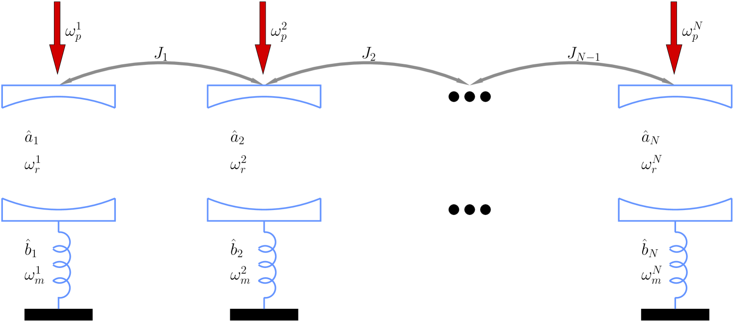
(b)

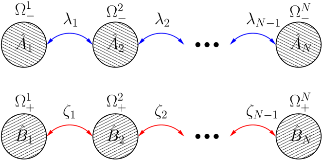
Figure 1: (Color online) (a) Sketch of an array of $N$ optomechanical cells, each of these cells consists of a mechanical mode of frequency $\omega_{m}^{n}$ coupled via radiation pressure to a cavity mode of frequency $\omega_{r}^{n}$. The optical mode is driven by a laser at frequency $\omega_{p}^{n}$ and cells are coupled by evanescent coupling between nearest neighbors cavities with hoping strength $J_{n}$. (b) Schematic of the effective model, two decoupled bosonic chains with polaritonic energies $\Omega_{-}^{n}$, $\Omega_{+}^{n}$ and neighbor-site hopping $\lambda_{n}$ and $\zeta_{n}$ respectively.

II The Model

We consider a one-dimensional array of $N$ optomechanical cells, each of these cells consists of a mechanical mode of angular frequency $\omega_{m}^{n}$ coupled via radiation pressure to a cavity mode of angular frequency $\omega_{r}^{n}$. In addition, we consider an external laser driving the optical mode at angular frequency $\omega_{p}^{n}$, as schematically depicted in Fig. 1(a).

Following the standard linearization procedure for driving optical modes in optomechanical cavities, we can recast the following Hamiltonian (in units of Planck constant, i.e., $\hbar=1$)

$$\hat{H}_{n}^{L}=-\Delta_{p}^{n}\hat{a}_{n}^{\dagger}\hat{a}_{n}+\omega_{m}^{n}\hat{b}_{n}^{\dagger}\hat{b}_{n}-G_{n}(\hat{b}_{n}+\hat{b}_{n}^{\dagger})(\hat{a}_{n}+\hat{a}_{n}^{\dagger}),$$ (1)

where, the mechanical (optical) mode of the $n$-th cell is associated with the bosonic operator $\hat{b}_{n}$ ($\hat{a}_{n}$); $\Delta_{p}^{n}=\omega_{p}^{n}-\omega_{r}^{n}$ is the pump detuning from cavity resonance, $g_{n}$ corresponds to the single-photon coupling rate and $G_{n}=\alpha_{n}g_{n}$ is the effective optomechanical coupling strength proportional to the laser amplitude.

Here the cells are coupled by evanescent coupling between nearest neighbors cavities with hoping strength $J_{n},$ an interaction described by

$$\hat{H}_{I}=\sum_{n=1}^{N-1}J_{n}(\hat{a}_{n}^{\dagger}\hat{a}_{n+1}+\hat{a}_{n+1}^{\dagger}\hat{a}_{n}).$$ (2)

As seen from the above Hamiltonian $\hat{H}_{n}^{L}$ (with $\Delta_{p}^{n}<0$), we can readily notice two linearly coupled quantum harmonic oscillators. To obtain the relevant decoupled effective Hamiltonian, we proceed to diagonalization of the Hamiltonian using the usual Bogoliubov transformation as following:

$$\hat{A}_{n}={} \mathcal{N}_{-}\left[\Delta_{1}^{n}\left(\Omega_{-}^{n}\right)\hat{a}_{n}^{{\dagger}}+\Delta_{2}^{n}\left(\Omega_{-}^{n}\right)\hat{b}_{n}^{{\dagger}}\right.$$

$$\left.+\Delta_{3}^{n}\left(\Omega_{-}^{n}\right)\hat{a}_{n}+\Delta_{4}^{n}\left(\Omega_{-}^{n}\right)\hat{b}_{n}\right],$$

$$\hat{B}_{n}={} \mathcal{N}_{+}\left[\Delta_{1}^{n}\left(\Omega_{+}^{n}\right)\hat{a}_{n}^{{\dagger}}+\Delta_{2}^{n}\left(\Omega_{+}^{n}\right)\hat{b}_{n}^{{\dagger}}\right.$$

$$\left.+\Delta_{3}^{n}\left(\Omega_{+}^{n}\right)\hat{a}_{n}+\Delta_{4}^{n}\left(\Omega_{+}^{n}\right)\hat{b}_{n}\right],$$ (3)

with eigenvalues

$$(\Omega_{\mp}^{n})^{2}={} \frac{{\Delta_{p}^{n}}^{2}+{\omega_{m}^{n}}^{2}}{2}$$

$$\mp\frac{1}{2}\sqrt{\left((\Delta_{p}^{n})^{2}-(\omega_{m}^{n})^{2}\right)^{2}-16G_{n}^{2}\Delta_{p}^{n}\omega_{m}^{n}},$$ (4)

where we have defined

$$\Delta_{1}\left(\Omega_{\mp}^{n}\right)={} 2G_{n}^{2}\omega_{m}^{n}-\left(\Omega_{\mp}-\omega_{m}^{n}\right)\left(\Omega_{\mp}^{n}-\left|\Delta_{p}^{n}\right|\right)\left(\Omega_{\mp}^{n}+\omega_{m}^{n}\right),$$

$$\Delta_{2}\left(\Omega_{\mp}^{n}\right)={} G_{n}\left[\left(\Omega_{\mp}-\left|\Delta_{p}^{n}\right|\right)\left(\Omega_{\mp}-\omega_{m}^{n}\right)\right],$$

$$\Delta_{3}\left(\Omega_{\mp}^{n}\right)={} 2G_{n}^{2}\omega_{m}^{n},$$

$$\Delta_{4}\left(\Omega_{\mp}^{n}\right)={} G_{n}\left(\Omega_{\mp}-\left|\Delta_{p}^{n}\right|\right)\left(\Omega_{\mp}+\omega_{m}^{n}\right),$$

and normalization

$$\frac{1}{\mathcal{N}_{n,\mp}^{2}}={} \left[\Delta_{3}\left(\Omega_{\mp}^{n}\right)\right]^{2}+\left[\Delta_{4}\left(\Omega_{\mp}^{n}\right)\right]^{2}$$

$$-\left[\Delta_{1}\left(\Omega_{\mp}^{n}\right)\right]^{2}-\left[\Delta_{2}\left(\Omega_{\mp}^{n}\right)\right]^{2}.$$ (5)

Therefore, the total Hamiltonian $\hat{H}=\hat{H}_{n}^{L}+\hat{H}_{I\text{ }}$ in the polariton basis can be rewrite as

$$\tilde{H}={} \sum_{n=1}^{N}\Omega_{{}^{-}}^{n}\hat{A}_{n}^{\dagger}\hat{A}_{n}+\Omega_{{}^{+}}^{n}\hat{B}_{n}^{\dagger}\hat{B}_{n}$$

$$+\sum_{n=1}^{N-1}(\lambda_{n}\hat{A}_{n}^{\dagger}\hat{A}_{n+1}+\zeta_{n}\hat{B}_{n}^{\dagger}\hat{B}_{n+1}+\rm{H.c.}),$$ (6)

with the effective tunneling strength

$$\lambda_{n}={} J_{n}\mathcal{N}_{n,-}\mathcal{N}_{n+1,-}\left[\Delta_{1}\left(\Omega_{-}^{n}\right)\Delta_{1}\left(\Omega_{-}^{n+1}\right)\right.$$

$$\left.+\Delta_{3}\left(\Omega_{-}^{n}\right)\Delta_{3}\left(\Omega_{-}^{n+1}\right)\right]$$

and

$$\zeta_{n}={} J_{n}\mathcal{N}_{n,+}\mathcal{N}_{n+1,+}\left[\Delta_{2}\left(\Omega_{+}^{n}\right)\Delta_{2}\left(\Omega_{+}^{n+1}\right)\right.$$

$$\left.+\Delta_{4}\left(\Omega_{+}^{n}\right)\Delta_{4}\left(\Omega_{+}^{n+1}\right)\right].$$

It is important to point out that in deriving the above expression, terms like $A_{i}^{\dagger}A_{i+1}^{\dagger}$ and $A_{i}^{\dagger}B_{i+1}$ have been neglected due to the usual rotating-wave approximation (RWA), which remains valid for

$$\Omega_{\mp}^{n},\left|\Omega_{+}^{n}-\Omega_{-}^{n}\right|\gg\sqrt{\sum_{n}^{N}\left\langle\hat{a}_{n}^{\dagger}\hat{a}_{n}\right\rangle+\left\langle\hat{b}_{n}^{\dagger}\hat{b}_{n}\right\rangle}(\lambda_{n}+\zeta_{n}).$$

Now, it is straightforward to observe under the above mapping that the original full Hamiltonian of a unidimensional array of optomechanical cells becomes equivalent to a Hamiltonian of two distinct bosonic chains, this Hamiltonian being the central result of this manuscript. Scenario schematically illustrated in Fig. 1(b). Because of the effective structure achieved above, i.e., two independent chains, we are now in position to take advantage of the well-known results on quantum state transfer.

As known from any state transfer scheme, the set of couplings parameters $\left\{\lambda_{n},\zeta_{n}\right\}$ as well as energies $\Omega_{\mp}^{n}$ defines the transfer time $\tau.$ Here, we point out that our protocol requires that the transfer time for both polaritons $\hat{A}^{\dagger}\hat{A}$ and $\hat{B}^{\dagger}\hat{B}$ has to be the same or at least an odd multiple of each other.

To illustrate this point, we will consider the red-detuned regime $\Delta_{p}^{n}\approx-\omega_{m}^{n}$, thus the Hamiltonian (1) can be simplified as

$$\hat{H}_{n}^{\rm{red}}=\omega_{m}^{n}(\hat{a}_{n}^{\dagger}\hat{a}_{n}+\hat{b}_{n}^{\dagger}\hat{b}_{n})-G_{n}(\hat{b}_{n}\hat{a}_{n}^{\dagger}+\hat{b}_{n}^{\dagger}\hat{a}_{n}).$$ (7)

To obtain the diagonal form of the above expression, we consider the operators

$$\hat{A}_{n}=\frac{(\hat{a}_{n}+\hat{b}_{n})}{\sqrt{2}},\qquad\hat{B}_{n}=\frac{(\hat{a}_{n}-\hat{b}_{n})}{\sqrt{2}}$$ (8)

with eigenvalues $\omega_{A}^{n}=\omega_{m}^{n}-G_{n}$ and $\omega_{B}^{n}=\omega_{m}^{n}+G_{n}$, respectively.

For the strongly off-resonant regime ($G_{n}\gg J_{n})$ together with the RWA, we can recast the following polariton Hamiltonian

$$\hat{H}={} \sum_{n=1}^{N}\left(\omega_{A}^{n}\hat{A}_{n}^{\dagger}\hat{A}_{n}+\omega_{B}^{n}\hat{B}_{n}^{\dagger}\hat{B}_{n}\right)$$

$$+\sum_{i=1}^{N-1}\frac{J_{n}}{\sqrt{2}}\left(\hat{A}_{n}^{\dagger}\hat{A}_{n+1}+\hat{B}_{n}^{\dagger}\hat{B}_{n+1}+\rm{H.c.}\right).$$ (9)

Now we proceed to choose a set of parameters that allows quantum state transfer. For instance, a straightforward set can be found in Ref. Nikolopoulos and Jex (2013) corresponding to $\omega_{m}^{n}=\omega_{m},G_{n}=G$ and $J_{n}=({J}/{\sqrt{2}})\sqrt{n(N-n)}$, which provides the same transfer time for each chain $\tau_{A}=\tau_{B}={\pi}/{J}$.

Therefore, regardless a relative phase depending on $\omega_{A}$ and $\omega_{B}$ which is fixed and known, and hence, it can be amended, any optomechanical state can be transferred only ensuring the $G\gg J$ regime together with $J_{n}=({J}/{\sqrt{2}})\sqrt{n(N-n)}$.

However, we stress that any other protocol could have been chosen for this purpose. For example, schemes based on eigenmodes, where one of many possibilities that permit quantum state transfer is the following set of parameters: $J_{1}=J_{N-1}=\lambda\ll J_{k}=J\ll G,k=2\ldots N-2,N$ being an odd number and $\omega_{m}^{n}=\omega_{m},G_{n}=G$.

On the other hand, on resonant schemes Plenio and Semião (2005); *PRL.2011.106.040505 the shorter transfer time possible corresponds to $\tau_{A}=\tau_{B}=(\pi/\lambda)\sqrt{2(N+1)}$, and for tunneling-like protocol Neto et al. (2012) with same parameters and conditions $\omega_{m}^{1}=\omega_{m}^{N}=\omega_{m}+\delta$ and $\lambda\ll\delta\ll J$, we obtain transfer times $\tau_{A}=\tau_{B}={N\pi\delta}/{2\lambda^{2}}$.

Finally, it is worth stressing that, the effect of a phononic hop term between neighboring sites only change the strength of $\lambda_{n}$ and $\zeta_{n}$.

III Dissipative mechanisms

In this section, in a step towards a more realistic model we take into account decoherence and dissipation. To fulfill this goal, we employ the standard formalism for open quantum systems, i.e., we solve the dynamics of the optomechanical array using the master equation in Lindblad form within the Born-Markov approximation.

Furthermore, we numerically investigate the effectiveness of our model computing the fidelity for the state transfer considering engineered hop couplings between cells where each cell is considered in the red-sideband regime.

The master equation for the composite coupled system is given as

$$\frac{d\hat{\rho}}{dt}={} -i\left[\hat{H},\hat{\rho}\right]$$ (10)

$$+\sum_{n=1}^{N}\frac{\kappa_{n}}{2}(1+\overline{n}_{c})\mathcal{D}\left[\hat{a}_{n}\right]\hat{\rho}+\frac{\kappa_{n}}{2}\overline{n}_{c}\mathcal{D}\left[\hat{a}_{n}^{\dagger}\right]\hat{\rho}$$

$$+\frac{\gamma_{n}}{2}(1+\overline{n}_{m})\mathcal{D}\left[\hat{b}_{n}\right]\hat{\rho}+\frac{\gamma_{n}}{2}\overline{n}_{m}\mathcal{D}\left[\hat{b}_{n}^{\dagger}\right]\hat{\rho},$$ (11)

where $\hat{H}=\sum_{n=1}^{N}\hat{H}_{n}^{\rm{red}}+\hat{H}_{I}$ and the Lindblad term

$$\mathcal{D}\left[\hat{O}\right]=2\hat{O}\rho\hat{O}^{\dagger}-\rho\hat{O}^{\dagger}\hat{O}-\hat{O}^{\dagger}\hat{O}\rho$$ (12)

takes into account the dissipative mechanisms of the optics (mechanics) in contact with a thermal reservoir with occupation number $\overline{n}_{c}$ $(\overline{n}_{m})$, where the photon (phonon) decay rate is given by $\kappa_{n}(\gamma_{n})$.

Figure 2: (Color online) The figure shows the dynamics of the transfer fidelity at time $\tau=\pi/J$ as a function of $G/J$. The states $|\phi_{+}\rangle=({1}/{\sqrt{2}})\left(|1,0\rangle+|0,1\rangle\right)$ and $|\Phi_{+}\rangle=({1}/{\sqrt{2}})\left(|2,0\rangle+|0,2\rangle\right)$ corresponds to the initial states of the sender.

Figure 3: (Color online) We illustrate the fidelity of the transfer process $(\tau=\pi/J)$ as a function of $\kappa/J$ (log-axis) for two mechanical phonon bath occupation number $\overline{n}_{m}=100$ and $\overline{n}_{m}=1$. To exhibit our findings, we consider the following feasible parameters in optomechanical crystals Chan et al. (2011) in the microwave regime; $\omega_{m}/2\pi=3.68\times 10^{9},\gamma/2\pi=35\times 10^{3}$, $\overline{n}_{c}=0.005$, $G=({J}/{4})\times 10^{2}=5\times 10^{9}$.

Needless to say that the first non-trivial quantum network in passive schemes is composed of four sites. Hence, for computational time purposes, we will exemplify our findings considering an array of four cells where the coupling fulfill $J_{n}=({J}/{\sqrt{2}})\sqrt{n(N-n)}$ and $\omega_{m}^{n}=\omega_{m}$.

To validate the polariton Hamiltonian (9), we present the closed evolution of the transfer fidelity at time $\tau=\pi/J$ as a function of $G/J$, see Fig. (2).

In order to compute the fidelity of the transferred quantum state, we solved the closed quantum system dynamics (running the simulation in QuTiP Johansson et al. (2012)) considering the sender initially in the state $|\phi_{+}\rangle=({1}/{\sqrt{2}})\left(|1,0\rangle+|0,1\rangle\right)$ or $|\Phi_{+}\rangle=({1}/{\sqrt{2}})\left(|2,0\rangle+|0,2\rangle\right)$ (we have used the following notation $|a,b\rangle=|a\rangle_{optics}\otimes|b\rangle_{mechanics}$), where all the other cells are in the vacuum state.

Moreover, for our illustrative red sideband detuning regime $(-\Delta_{p}\approx\omega_{m}\gg\gamma,\kappa)$ a well-known stability condition Genes et al. (2009) given by $G<({1}/{2})\sqrt{\omega_{m}^{2}+{(\gamma^{2}+\kappa^{2})}/{4}}$ come into sight, and therefore it must be observed throughout the quantum state transfer protocol. On the other hand, in order to achieve a fidelity value close to the unity, G has to be $G\approx({J}/{4})\times 10^{2}$ (as seen in Fig. 2). The effect of both the stability condition (being an upper bound for G), as well as the effectiveness of the fidelity ($\mathcal{F(\tau)}\rightarrow 1$), have as a result the limitation of the maximum coupling strength $J_{n={N}/{2}}=N{J}/{4}$ and consequently the maximum number of cells.

In Fig. 3, we compute the fidelity for the transfer of an initial quantum state given by $|\phi_{+}\rangle$ as a function of $\kappa/J$ for two different mechanical phonon bath occupation number $\overline{n}_{m}=100$ and $\overline{n}_{m}=1$, where we have used the following currently experimental parameters in optomechanical crystals Chan et al. (2011) in the GHz regime; $\omega_{m}/2\pi=3.68\times 10^{9}$, $\gamma/2\pi=35\times 10^{3}$, $\overline{n}_{c}=0.005$, $G=({J}/{4})\times 10^{2}=5\times 10^{9}$. The high fidelity shown in Fig. 3 up to $J=10\kappa$ is an expected result, since $k_{B}T<\hbar\omega_{m}$, and the threshold for coherent operations take place when $\max(J_{n})=\max(\gamma_{n},\kappa_{n})$. Thus, to achieve transfer fidelities close to unity for an array with $N=100$ cells (with the same set of parameters considered above), we can then estimate the cavity linewidth as $\kappa\sim 10^{5}$.

Finally, we point out that the hopping coupling reported in Heinrich et al. (2011) is in the range of THz. Hence, to achieve the inequality $J<G$ within the stability region, we should engineered optomechanical arrays with larger lattice spacing and/or mechanical modes with frequencies above THz, being this last a challenging experimental scenario.

IV Conclusion

We have thus advanced a theoretical proposal for quantum state transfer in optomechanical arrays. Our proposal relies on a general scheme illustrated by polariton transformation of the linearized Hamiltonian (6) that allow us to obtain an effective Hamiltonian of two decoupled bosonic networks.

The central result of the present manuscript is the derivation of the polariton Hamiltonian (6), where we can bring previous results from quantum state transfer protocols in bosonic networks. Specifically, we can apply any type of quantum state transfer scheme with an extra additional condition, namely, that the rate between the transfer times of both decoupled polaritonic chains must be an odd number. Furthermore, we analyze the effects of dissipation and a possible experimental implementation of our proposal in the red-sideband regime with experimental accessible parameters.

It is also important to point out that —although not reported explicitly in this work— the linearization of the non-linear optomechanical Hamiltonian does not constitute a major restriction. For instance, for driven optomechanical systems in the strong single-photon regime, we can both transfer information encoded in polariton states arising from ion trap-like Hamiltonian Xu et al. (2013) as well as dark states in optomechanical systems Xu and Law (2013).

Moreover, even though we used a one-dimensional array in this work, any other topology might be consider, such as lattices (2D) or crystals (3D) setups.

In addition, other interesting aspects to study are the “pretty good state transfer” schemes in Ref. Nikolopoulos and Jex (2013), and the generation of long distance quantum entanglement between sites Neto et al. (2012).

References

- Nielsen and Chuang (2010) M. A. Nielsen and I. I. Chuang, Quantum computation and quantum information (Cambridge Univ. Press, 2010).
- Kimble (1998) H. J. Kimble, Phys. Scr. 1998, 127 (1998).
- Myatt et al. (2000) C. J. Myatt, B. E. King, Q. A. Turchette, C. A. Sackett, D. Kielpinski, W. M. Itano, C. Monroe, and D. J. Wineland, Nature 403, 269 (2000).
- Mandel et al. (2003) O. Mandel, M. Greiner, A. Widera, T. Rom, T. W. Hansch, and I. Bloch, Nature 425, 937 (2003).
- Kane (1998) B. E. Kane, Nature 393, 133 (1998).
- Loss and DiVincenzo (1998) D. Loss and D. P. DiVincenzo, Phys. Rev. A 57, 120 (1998).
- Nikolopoulos and Jex (2013) G. Nikolopoulos and I. Jex, eds., Quantum Science and Technology (Springer Berlin Heidelberg, 2013).
- Christandl et al. (2004) M. Christandl, N. Datta, A. Ekert, and A. J. Landahl, Phys. Rev. Lett. 92, 187902 (2004).
- Kay (2006) A. Kay, Phys. Rev. A 73, 032306 (2006).
- Briegel et al. (1998) H.-J. Briegel, W. Dür, J. I. Cirac, and P. Zoller, Phys. Rev. Lett. 81, 5932 (1998).
- Burgarth and Bose (2005) D. Burgarth and S. Bose, New J. Phys. 7, 135 (2005).
- Tsomokos et al. (2007) D. I. Tsomokos, M. J. Hartmann, S. F. Huelga, and M. B. Plenio, New J. Phys. 9, 79 (2007).
- Liu et al. (2002) W. M. Liu, W. B. Fan, W. M. Zheng, J. Q. Liang, and S. T. Chui, Phys. Rev. Lett. 88, 170408 (2002).
- Polkovnikov (2003) A. Polkovnikov, Phys. Rev. A 68, 033609 (2003).
- Plenio et al. (2004) M. B. Plenio, J. Hartley, and J. Eisert, New J. Phys. 6, 36 (2004).
- Yung and Bose (2005) M.-H. Yung and S. Bose, Phys. Rev. A 71, 032310 (2005).
- Kostak et al. (2007) V. Kostak, G. M. Nikolopoulos, and I. Jex, Phys. Rev. A 75, 042319 (2007).
- Aspelmeyer et al. (2014) M. Aspelmeyer, T. J. Kippenberg, and F. Marquardt, Rev. Mod. Phys. 86, 1391 (2014).
- Bose et al. (2007) S. Bose, D. G. Angelakis, and D. Burgarth, Journal of Modern Optics, J. Mod. Opt. 54, 2307 (2007).
- de Moraes Neto et al. (2011) G. D. de Moraes Neto, M. A. de Ponte, and M. H. Y. Moussa, Phys. Rev. A 84, 032339 (2011).
- Eichenfield et al. (2009) M. Eichenfield, J. Chan, R. M. Camacho, K. J. Vahala, and O. Painter, Nature 462, 78 (2009).
- Chang et al. (2011) D. E. Chang, A. H. Safavi-Naeini, M. Hafezi, and O. Painter, New J. Phys. 13, 023003 (2011).
- Heinrich et al. (2011) G. Heinrich, M. Ludwig, J. Qian, B. Kubala, and F. Marquardt, Phys. Rev. Lett. 107, 043603 (2011).
- Tomadin et al. (2012) A. Tomadin, S. Diehl, M. D. Lukin, P. Rabl, and P. Zoller, Phys. Rev. A 86, 033821 (2012).
- Akram et al. (2012) U. Akram, W. Munro, K. Nemoto, and G. J. Milburn, Phys. Rev. A 86, 042306 (2012).
- Wang and Clerk (2012) Y.-D. Wang and A. A. Clerk, Phys. Rev. Lett. 108, 153603 (2012).
- Sete and Eleuch (2015) E. A. Sete and H. Eleuch, Phys. Rev. A 91, 032309 (2015).
- Schmidt et al. (2012) M. Schmidt, M. Ludwig, and F. Marquardt, New J. Phys. 14, 125005 (2012).
- Plenio and Semião (2005) M. B. Plenio and F. L. Semião, New J. Phys. 7, 73 (2005).
- Yao et al. (2011) N. Y. Yao, L. Jiang, A. V. Gorshkov, Z.-X. Gong, A. Zhai, L.-M. Duan, and M. D. Lukin, Phys. Rev. Lett. 106, 040505 (2011).
- Neto et al. (2012) G. D. M. Neto, M. A. de Ponte, and M. H. Y. Moussa, Phys. Rev. A 85, 052303 (2012).
- Xu et al. (2013) X.-W. Xu, H. Wang, J. Zhang, and Y.-x. Liu, Phys. Rev. A 88, 063819 (2013).
- Xu and Law (2013) G.-F. Xu and C. K. Law, Phys. Rev. A 87, 053849 (2013).
- Chan et al. (2011) J. Chan, T. P. M. Alegre, A. H. Safavi-Naeini, J. T. Hill, A. Krause, S. Groblacher, M. Aspelmeyer, and O. Painter, Nature 478, 89 (2011).
- Johansson et al. (2012) J. Johansson, P. Nation, and F. Nori, Comput. Phys. Commun. 183, 1760 (2012).
- Genes et al. (2009) C. Genes, A. Mari, D. Vitali, and P. Tombesi, in Advances in Atomic Molecular and Optical Physics, Vol. Volume 57 (Academic Press, 2009) pp. 33–86.