Momentum-dependent pseudo-spin dimers of coherently coupled bosons in optical lattices

Abstract

We study the two-body bound and scattering states of two particles in a one dimensional optical lattice in the presence of a coherent coupling between two internal atomic levels. Due to the interplay between periodic potential, interactions and coherent coupling, the internal structure of the bound states depends on their center of mass momentum. This phenomenon corresponds to an effective momentum-dependent magnetic field for the dimer pseudo-spin, which could be observed in a chirping of the precession frequency during Bloch oscillations. The essence of this effect can be easily interpreted in terms of an effective bound state Hamiltonian. Moreover for indistinguishable bosons, the two-body eigenstates can present simultaneously attractive and repulsive bound-state nature or even bound and scattering properties.

I Introduction

In the recent years it has been demonstrated that ultracold atoms loaded in optical lattices provide an ideal realization of lattice Hamiltonians jaksch2005cold ; RevModPhys.80.885 . The control of the system parameters, in particular of the ratio between interactions and kinetic energy, has allowed the experimental achievement of the most famous Mott insulator to superfluid phase transition in 2002 Bloch-MottSF . From there on, the number of implementations of Hubbard-like models using cold gases in optical lattices has undergone an incredible growth (see, e.g., BookMaciek ): it is now possible to mimic single- and multi-species Bose and Fermi-Hubbard models, extended Hubbard models by using dipolar gases FranceEHM , and spin chain models greiner2011 ; esslinger2013 ; blochXXZ . More recently, Hubbard models characterised by non-trivial topology, synthetic magnetic field, artificial gauges BlochButterfly ; KetterleButterfly , or synthetic dimensions Leosintdim have been realized.

Most of the theoretical studies on lattice Hamiltonians regard many-body or single particle properties, especially in the case of non trivial topology. On the other hand, lattice Hamiltonians show interesting features also as far as the few body physics is concerned. Indeed, when the effect of interactions is combined with the presence of the lattice, composite objects on a lattice behave very differently with respect to their counterpart in free space MattisFewBody . First of all the dispersion relation, i.e. the effective mass of bound particles depends on the binding energy. This is due to the impossibility in the lattice of separating the relative motion and the center-of-mass degrees of freedom. Moreover the spectrum of the scattering states, the so-called essential spectrum, is bounded from below and from above. Therefore bound states can exist both for attractive and for repulsive interactions Hubbard1963 ; MattisFewBody . The existence of “exotic” repulsive bound pairs (RBP) has been directly observed for the first time a few years ago for an ultra-cold Bose gas in an optical lattice winkler2006repulsively .

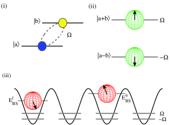
Figure 1: Schematic representation of two coherently coupled interacting bosons in an optical lattice for $U_{a}=U_{b}=U$: (i) two internal levels $|{a}\rangle\,$ and $|{b}\rangle\,$ coherently coupled by a resonant coupling $\Omega$; (ii) single-particle eigenstates of $\Omega$ at energies $\pm\Omega$ provided by the internal state superpositions $|{a\pm b}\rangle\,$; in the Bloch sphere representation, the two single-particle states $|{a\pm b}\rangle\,$ point respectively in the positive and negative vertical direction; (iii) repulsive lower and upper two-body bound states respectively at energies $E_{BS}^{l,u}$: for $U=U_{ab}$ the dimers are formed by both atoms in the internal states $|{a\pm b}\rangle\,$, namely in the two-body internal states $|{\pm}\rangle\,$; in the Bloch sphere representation for the two-body internal states, the states $|{\pm}\rangle\,$ corresponds to a pseudo-spin pointing respectively in the positive and negative vertical direction; for $U\neq U_{ab}$ the internal wavefunctions of the dimers are modified and the corresponding pseudo-spins are rotated.

In this work, we consider two atoms with two coherently coupled internal levels in a one dimensional (1D) optical lattice. The two-body properties of this system can be investigated analytically, allowing for a clear understanding of the interplay between the exchange term (phase coupling) and the intra- and inter-species interactions (density coupling). The bound states of the system can be described in terms of a pseudo-spin wavefunction. Thanks to its spinorial structure, the bound states can, in certain regimes, show the co-presence of repulsive and attractive character or the co-presence of free (delocalized) and bound (localized) nature. Those features are absent in the single species situation. Moreover, we show that an effetive momentum-dependent magnetic field emerges for the pseudo-spin of the dressed dimers, by means of a coupling between the internal state of the bound state and its center-of-mass motion. The emergent coupling between internal and external degrees of freedom for the bound states is due to the different dispersion relations of the bare dimers in the different coupling channels and is very easily understood in terms of dressed bound states. The same effect also emerges in a dimer of two distinguishable particles, provided that at least one of them possesses two coherently coupled internal levels.

The paper is organised as follows: In Sect. II we describe the model and make the link to the single species repulsively bound pairs. We introduce the concept of momentum-dependent internal wavefunction for the dimers. We present an intuitive explanation of the physics behind this effect using an effective Hamiltonian and an effective pseudo-spin picture. In Sect. III, we solve analytically our model via a Lippmann-Schwinger treatment. We investigate in detail the properties of the bound states and discuss the effect of Bloch oscillations on the dimer pseudo-spin dynamics at the semiclassical level. We describe in detail the case of hybridized bound and scattering states, which are not present in the analogous single species model. In Sect. IV, we generalize our results in the presence of species-dependent hopping and intra-species interaction and compare the effective model with exact diagonalization results. In Sect. V, we show that analogous results are obtained for dimers of two distinguishable particles, as long as one of them has two coherently coupled internal levels. The experimental implementation and relevance of our work in the cold-gases context is discussed in the conclusions.

II Model and Results

We consider a two-component single-band Bose-Hubbard model with an exchange term between the two species, characterized by a frequency $\Omega$. In second quantization the Hamiltonian reads

$$\hat{H}=\hat{H}_{kin}+\hat{H}_{int}+\hat{H}_{\Omega},$$ (1)

where

$$\hat{H}_{kin} = -J_{a}\sum_{\langle i,j\rangle}\hat{a}^{\dagger}_{i}\hat{a}_{j}-J_{b}\sum_{\langle i,j\rangle}\hat{b}^{\dagger}_{i}\hat{b}_{j},$$ (2)

$$\hat{H}_{int} = \sum_{i}\left(\frac{U_{a}}{2}\hat{n}_{i}^{a}(\hat{n}_{i}^{a}-1)+\frac{U_{b}}{2}\hat{n}_{i}^{b}(\hat{n}_{i}^{b}-1)+U_{ab}\hat{n}_{i}^{a}\hat{n}_{i}^{b}\right),$$

$$\hat{H}_{\Omega} = \sum_{i}\Omega(\hat{a}_{i}^{\dagger}\hat{b}_{i}+\hat{b}_{i}^{\dagger}\hat{a}_{i}).$$

The operators $\hat{a}_{i}$ ($\hat{a}_{i}^{\dagger}$) and $\hat{b}_{i}$ ($\hat{b}_{i}^{\dagger}$) are the annihilation (creation) operators for a particle on site $i$ in the internal state $a$ and $b$, respectively. In this work, we set the lattice constant $d=1$.

A possible realization of model (1) can be provided by bosonic atoms in a 1D deep optical lattice, with two hyperfine states resonantly coupled via an external laser field. At the many-body level a number of properties of this model in different regimes have been already studied by means of bosonization techniques or using Density Matrix Renormalization Group numerical approaches (see, e.g., GiamarchiCC ; RecatiCCLattice ; McCullochCC ). In the present work we focus instead on the two-body physics and in particular on the bound states properties.

Let us first recall that in a single species 1D Bose-Hubbard Hamiltonian an on-site interaction $U_{\alpha}$ creates a dimer at energy

$$E^{\alpha}_{K}={\rm sign}(U_{\alpha})\sqrt{U_{\alpha}^{2}+16J^{2}\cos^{2}\left(\frac{K}{2}\right)},$$ (3)

where $K$ is the center-of-mass momentum. Depending on the sign of the interaction parameter $U_{\alpha}$, the bound state lies above or below the scattering states, whose energies define the essential spectrum $\Gamma_{ess}(K)=[-4J\cos(K/2),4J\cos(K/2)]$ (see, e.g., ValienteHM ). For $U_{\alpha}>0$, the two-body bound state is usually referred to as repulsively-bound pair winkler2006repulsively . The intuitive explanation behind repulsively bound pairs is provided by the fact that the interaction energy of a bound state cannot be converted into kinetic energy, due to the limited energy bandwidth. The dimer has a non-trivial dispersion relation, which becomes more and more flat for increasing interactions (see, e.g., MattisFewBody and references therein). For $|U_{\alpha}|\gg J$, the curvature of the dispersion relation at $K=0$, proportional to the inverse effective mass, is related to two-body hopping in second order perturbation theory $J_{eff}\propto J^{2}/U_{\alpha}$.

If we have two species $a$ and $b$ without coherent coupling, i.e. $\Omega=0$ in Eq. (2), there is a single bound state at energy $E^{\alpha}_{K}$ given, for $J_{a}=J_{b}=J$, by Eq. (3) with $U_{\alpha}$ replaced by $U_{aa},U_{bb}$ or $U_{ab}$, depending on whether the two particles are in the same or in different internal states. The bound state wavefunction can be written as $\Psi^{\alpha}_{K}(r)\;|\alpha\rangle$, where $\Psi^{\alpha}_{K}(r)$ is the relative motion wavefunction and $|{\alpha}\rangle\,\in\mathcal{B}_{int}$ describes the internal composition of the bound state, with

$$\mathcal{B}_{int}=\left\{\begin{split}|{2_{a},0_{b}}\rangle\,,\\ |{1_{a},1_{b}}\rangle\,,\\ |{0_{a},2_{b}}\rangle\,.\\ \end{split}\right.$$ (4)

The structure of the eigenfunctions is very simple because the internal state composition $|\alpha\rangle$ does not depend on $K$ .

Adding a finite $\Omega$ leads to a mixing of the previously described bound states. Neglecting for the moment the presence of the scattering continuum and its influence on the bound states, let us define for the bound states an effective Hamiltonian whose diagonal elements are given by the bound state dispersions $E^{\alpha}_{K}$ in Eq. (3). Assuming that the bound state wavefunctions $\Psi_{K}^{\alpha}(r)$ do not depend strongly on $|\alpha\rangle$, the exchange term provides the off-diagonal matrix elements $\langle 2_{a},0_{b}|{\hat{H}}_{\Omega}|1_{a},1_{b}\rangle=\langle 1_{b},1_{b}|{\hat{H}}_{\Omega}|0_{a},2_{b}\rangle=\sqrt{2}\Omega$. Hence for each value of $K$, one obtains an Hamiltonian of an effective $\Lambda$-system which reads

$$H_{eff}(K) = {\bar{E}_{K}}+\begin{pmatrix}\delta_{K}&\sqrt{2}\Omega&0\\ \sqrt{2}\Omega&\Delta_{K}&\sqrt{2}\Omega\\ 0&\sqrt{2}\Omega&-\delta_{K}\end{pmatrix},$$ (5)

with $2{\bar{E}_{K}}=E^{a}_{K}+E^{b}_{K}$, $2\delta_{K}=E^{a}_{K}-E^{b}_{K}$, $\Delta_{K}=E^{ab}_{K}-{\bar{E}_{K}}$.

We postpone to Sect. IV the discussion of the general case $J_{a}\neq J_{b}$ and $U_{a}\neq U_{b}$ and, for the sake of simplicity, we consider in most of the paper the $\mathbf{Z}_{2}$ symmetric situation where $J_{a}=J_{b}=J$ and $U_{a}=U_{b}=U$. In that case, $\bar{E}_{K}=E^{a}_{K}=E^{b}_{K}$, $\delta_{K}=0$, $\Delta_{K}=E^{ab}_{K}-{\bar{E}_{K}}$ and the diagonalization of the effective Hamiltonian leads to two coupled bright states and a dark state not affected by the coupling $\Omega$. The dark state, at energy $E_{eff}^{0}(K)={\bar{E}_{K}}$, is the coherent superposition of the two intra-species dimers providing the Bell state ${|{0}\rangle\,}=(|{2_{a},0_{b}}\rangle\,-|{0_{a},2_{b}}\rangle\,)/\sqrt{2}$ and does not depend on the center-of-mass momentum. The bright upper ($u$) and lower ($l$) bound states, have energies

$$E_{eff}^{u,l}(K)={\bar{E}_{K}}+\frac{1}{2}\left(\Delta_{K}\pm\sqrt{\Delta_{K}^{2}+16\Omega^{2}}\right).$$ (6)

Their internal wavefunction can be written as

$$\begin{split}{|{u;l}\rangle\,}_{K}\propto&(|{2_{a},0_{b}}\rangle\,+|{0_{a},2_{b}}\rangle\,)+\\ &\sqrt{2}\left(\frac{\Delta_{K}}{2\Omega}\pm\sqrt{\left(\frac{\Delta_{K}}{2\Omega}\right)^{2}+1}\right)|{1_{a},1_{b}}\rangle\,.\end{split}$$ (7)

In general the internal composition of the bright states does depend on the center-of-mass momentum. This is physically due to the fact that interactions try to preserve polarised bound states, while coherent coupling prefers to force the atoms in a balanced superposition of the two internal levels. From Eq. (7) and the reasoning above, in order for the momentum-dependence of the bound states to be pronounced, one needs relevant bare intra- and inter-species energy differences $\Delta_{K}$ combined with $\Omega,U$ and $U_{ab}$ not much larger than the hopping parameter $J$. Conversely, the condition $U=U_{ab}$, i.e. $\Delta_{K}=0$, defines the $U(1)$ symmetric case , where also the bright bound states are characterized by the $K$-indipendent internal wavefunctions ${|{\pm}\rangle\,}$, corresponding to both atoms in the superpositions $|{a\pm b}\rangle\,$, eigenstates of $\hat{H}_{\Omega}$ (see Eq. (13)).

The effective Hamiltonian in Eq. (5) assumes bound states well separated from the continuum. For repulsive (attractive) interactions it can happen that the lower (upper) bound state energy enters the upper (lower) scattering continuum. Even in this case, many of the conclusions provided for the upper (lower) bound state by the effettive model may still remain valid (see Sect.III.1). However, as we will show in Sect. III.2, interesting phenomena can occur due to the hybridisation between lower (upper) bound states and scattering states. In particular, the eigenfunctions present scattering character when projected on the upper (lower) two-body eigenstate of ${\hat{H}}_{\Omega}$ and bound state character when projected onto the orthogonal lower (upper) eigenstate of ${\hat{H}}_{\Omega}$.

While we are mainly interested in atoms satisfying Bose statistics, the previous results apply also for two distinguishable particles. In this case it is enough that a Rabi coupling between two different internal levels is present for one of the particles. The effective Hamiltonian, as well as the exact results obtained via Lippmann-Schwinger approach, can be easily extended (see Sect.V). The advantage is that using two different atomic species or isotopes the range of available parameters could be broader, possibly allowing to obtain a larger momentum dependence of the bound states.

II.1 $S=1/2$ pseudo-spin dynamics

Before discussing the exact solution, let us describe the effect of Bloch oscillations on the pseudo-spin of the dimers. As discussed in Sect. III, in the $\mathbf{Z}_{2}$ symmetric case, the bound state Hamiltonian in Eq. (5) separates in a dark manifold and in a two-dimensional bright manifold spanned by the states ${|{\pm}\rangle\,}$ (see Eq. (13)). Introducing a pseudo-spin notation for the $|{\pm}\rangle\,$ states, the dynamics is driven at each $K$ by the Hamiltonian

$$H^{\prime}_{eff}(K)=\bar{E}_{K}+\frac{\Delta_{K}}{2}+2\Omega\sigma_{z}-\frac{\Delta_{K}}{2}\sigma_{x}.$$ (8)

The density matrix for a pseudo-spin $S=1/2$ can be written as $\rho=(1+\mathbf{S}\cdot\sigma)/2$. From Eq. (8), the equations of motion for the pseudo-spin, describing a dimer wavepacket with center of mass momentum $K$, correspond at a semiclassical level to the dynamics of a spin in an effective magnetic field

$${d\over dt}\mathbf{S}=\mathbf{h^{\prime}}_{K}\times\mathbf{S},$$ (9)

with $\mathbf{h^{\prime}}_{K}=(-\Delta_{K},0,4\Omega)$ .

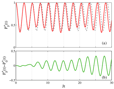
Figure 2: Effective pseudo-spin dynamics for a system prepared in the two-body state $|{+}\rangle\,$ at $t=0$ for $U=J$, $U_{ab}=J/4$ and $\Omega=J$: (a) probability $P^{+}_{F}(t)$ of finding the system in state $|{+}\rangle\,$ in the presence of Bloch oscillations driven by a constant force $F=J$ (red line) compared to $P^{+}_{0}(t)$ in the absence of driving force (grey dashed line); (b) difference of the two probabilities $P^{+}_{F}(t)-P^{+}_{0}(t)$ (green line).

In Fig. 2, we plot the probability of finding the system in the two-body state $|{+}\rangle\,$, corresponding to the expectation value of $S_{z}$, for two particles prepared at $t=0$ in the state $|{+}\rangle\,$ at $K=0$. The pseudo-spin of a wavepacket with center of mass momentum $K$ rotates at a frequency $\omega_{L}=h^{\prime}(K)$ and $\langle S_{z}\rangle$ oscillates periodically in time. If the center of mass momentum $K$ varies in time, the consequent spin dynamics results in a spin precessing in an effective time-dependent magnetic field $h^{\prime}(K(t))$. In particular, Bloch oscillations created by an external force $F$ induce, in the semiclassical approximation, a linear variation in time of the center of mass moment $K(t)=Ft/\hbar$. The effect of the time-dependent $K$ manifests itself in a chirping of the precession frequency $\omega_{L}(t)=h^{\prime}(K(t))$ and in the appearance of a beating frequency, as reported Fig. 2 (red line in (a) and green line in (b)).

The previous treatment is useful and illustrative in the $\mathbf{Z}_{2}$ symmetric case and taking as initial condition a state belonging to the bright manifold. In the more general case, e.g., starting with a bound state $|2_{a},0_{b}\rangle$, or in the asymmetric case for which also the dark state is involved in the dynamics, an effective $S=1$ treatment is required. Namely one can write directly the effective Hamiltonian in Eq. (5) using the Gell-Mann matrices $\Lambda_{i}$, $i=1\dots 8$ as

$$H_{eff}(K)={\bar{E}_{K}}+\frac{\Delta_{K}}{3}+\sum_{i=1}^{8}h_{i}(K)\Lambda_{i},$$ (10)

where we introduced the pseudo-magnetic field

$$\mathbf{h}(K)=$$ (11)

$$(\sqrt{2}\Omega,0,(\delta_{K}-\Delta_{K})/2,0,0,\sqrt{2}\Omega,0,\sqrt{3}(\Delta_{K}/3+\delta_{K})/2).$$

The density matrix can now be written as $\rho=(1+\mathbf{S}\cdot\Lambda)/3$. The equations of motion for the spin of a wave packet of center of mass momentum $K$ become

$${d\over dt}S_{k}=\sum_{l,\;j=1}^{8}f^{klj}h_{l}(K)S_{j},$$ (12)

where we use the standard notation for antisymmetric tensor $f^{klj}$ defining the $SU(3)$ Lie algebra $[\Lambda_{l},\Lambda_{j}]=if^{ljk}\Lambda_{k}$.

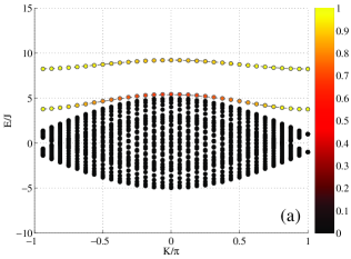
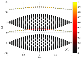
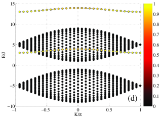
Figure 3: Spectrum for $J_{a}=J_{b}=J$ and: (a) $U_{a}=U_{b}=8J$, $U_{ab}=4J$, $\Omega=0.5J$; (b) $U_{a}=U_{b}=8J$, $U_{ab}=J$, $\Omega=2.5J$; (c) $U_{a}=U_{b}=8J$, $U_{ab}=4J$, $\Omega=2.5J$; (d) $U_{a}=U_{b}=8J$, $U_{ab}=8J$, $\Omega=2.5J$. For each eigenstate, the population at relative distance $r=0$ is plotted in color scale. The dashed lines are the bound-state energy predictions of the effective model. For clarity, in these figures the dark state spectrum is not shown.

III Lippmann-Schwinger formalism

In this section, we solve exactly the two-body problem for Hamiltonian (1) using the Lippmann-Schwinger formalism. We restrict ourselves to the $\mathbf{Z}_{2}$ symmetric case of $J_{a}=J_{b}$ and $U_{a}=U_{b}$, which allows for compact analytical expressions and a clear interpretation of the results. The more general case is treated in Sect. IV where the results are obtained by exact diagonalisation and a generalized effective model.

In order to write the Lippmann-Schwinger equations, it is convenient to define $\hat{H}_{kin}+\hat{H}_{\Omega}$ to be the free Hamiltonian. Since we are considering $J_{a}=J_{b}$, so that $[\hat{H}_{kin},\hat{H}_{\Omega}]=0$, the most suited basis is given by the 2-body internal eigenstates of $\hat{H}_{\Omega}$

$$\mathcal{B}_{\Omega}=\left\{\begin{split}|{+}\rangle\,&=\frac{|{2_{a},0_{b}}\rangle\,+\sqrt{2}|{1_{a},1_{b}}\rangle\,+|{0_{a},2_{b}}\rangle\,}{2},\\ |{-}\rangle\,&=\frac{|{2_{a},0_{b}}\rangle\,-\sqrt{2}|{1_{a},1_{b}}\rangle\,+|{0_{a},2_{b}}\rangle\,}{2},\\ |{0}\rangle\,&=\frac{|{2_{a},0_{b}}\rangle\,-|{0_{a},2_{b}}\rangle\,}{\sqrt{2}}.\\ \end{split}\right.$$ (13)

The state $|{0}\rangle\,$ corresponds to the dark state discussed above. Conversely, as it will become clear in Eq.(15), the states $|{\pm}\rangle\,$ are coupled to each other by the interaction term. The essential spectrum $\Gamma^{\Omega}_{ess}=\cup_{\sigma}\Gamma^{\sigma}_{ess}$ is provided by union of the three scattering spectra $\Gamma^{\sigma}_{ess}(K)=\Omega_{\sigma}+\Gamma_{ess}(K)$ obtained by shifting the essential spectrum of a single component Bose-Hubbard model by $\Omega_{\sigma}=2\sigma\Omega$ for $\sigma=+,\,0,\,-$.

To describe the external degrees of freedom, we follow the standard procedure of introducing the centre-of-mass coordinate $R=(x_{1}+x_{2})/2$ and the relative coordinate $r=x_{1}-x_{2}$ for two particles at lattice positions $x_{1}$ and $x_{2}$. The center of mass and relative coordinates do not separate on a lattice, but still the center of mass momentum $K=k_{1}+k_{2}$ is a good quantum number. Therefore, the eigenstates can be written as spinor wavefunctions $\sum_{\sigma}e^{iKR}\psi^{\sigma}_{K}(r)|{\sigma}\rangle\,$ with $|{\sigma}\rangle\,\in\mathcal{B}_{\Omega}$. Inserting this Ansatz in Eq. (1), we get the discrete Schrödinger equation for the relative motion

$$\begin{split}\hat{H_{r}}\psi_{K}^{\sigma}(r)=\left[-2J\tilde{\Delta}_{r}^{K}+\Omega_{\sigma}\right]\psi_{K}^{\sigma}(r)+\sum_{\sigma^{\prime}}U_{\sigma,\sigma^{\prime}}\delta_{r,0}\psi_{K}^{\sigma^{\prime}}(r),\end{split}$$ (14)

where $\delta_{r,0}$ is the Kronecker-delta and the parametric dependence of the kinetic energy on $K$ is contained in the discrete gradient $\tilde{\Delta}_{r}^{(K)}f(r)=\cos(K/2)[f(r+1)+f(r-1)]$. The interaction matrix reads

$$U_{\sigma,\sigma^{\prime}}=\left(\begin{array}[]{cccc}\frac{U+U_{ab}}{2}&\frac{U-U_{ab}}{2}&0\\ \frac{U-U_{ab}}{2}&\frac{U+U_{ab}}{2}&0\\ 0&0&U\end{array}\right).$$ (15)

As already mentioned, interactions mix only the states $|{\pm}\rangle\,$ spanning the so-called bright manifold, while the dark state $|{0}\rangle\,$ is completely decoupled.

For each value of $K$, let us call $H_{0}^{(K)}=-2J\tilde{\Delta}_{r}^{K}+\Omega_{\sigma}$ the free Hamiltonian, with eigenstates $|\Phi_{K}\rangle$ satisfying ${\hat{H}}_{0}^{(K)}|\Phi_{K}\rangle=E|\Phi_{K}\rangle$. The formal solution of the Lippmann-Schwinger equation reads

$$|\psi_{K}\rangle=|\Phi_{K}\rangle+{\hat{G}}_{K}(E){\hat{H}}_{int}|\psi_{K}\rangle,$$ (16)

where ${\hat{G}}_{K}(E)=(E-\hat{H}_{0}^{(K)}+i\eta)^{-1}$ is the free retarded Green’s function.

III.1 Bound states

Bound states do exist if the homogeneous equation $|\psi_{K}\rangle={\hat{G}}_{K}(E){\hat{H}}_{int}|\psi_{K}\rangle$ has non-zero solutions, or equivalently if there exist values $E_{BS}\notin\Gamma^{\Omega}_{ess}$ such that

$$\det[\mathbbm{1}-\hat{G}_{K}(E_{BS})\,\hat{H}_{int}]=0.$$ (17)

In our case the Green’s function components read

$$G_{K}^{\sigma}(r,0,E_{BS})=\frac{{\text{sgn}}(E_{BS}-\Omega_{\sigma})(\lambda_{K}^{\sigma})^{|r|}}{\sqrt{(E_{BS}-\Omega_{\sigma})^{2}-\beta_{K}^{2}}},$$ (18)

where we define $\beta_{K}=4J\cos(K/2)$ and

$$\lambda_{K}^{\sigma} \equiv -\frac{E_{BS}-\Omega_{\sigma}}{\beta_{K}}+$$

$${\text{sgn}}(E_{BS}-\Omega_{\sigma})\sqrt{\left(\frac{E_{BS}-\Omega_{\sigma}}{\beta_{K}}\right)^{2}-1}.$$

The dark state gives rise to a bound state equivalent to the one of the single species Hubbard model with $U_{\alpha}=U$. The bright states are coupled by the interactions and the condition for the existence of bound states reads

$$\Bigg{|}\begin{array}[]{cc}1-G_{K}^{+}(0,0,E_{BS})\frac{U+U_{ab}}{2}&G_{K}^{+}(0,0,E_{BS})\frac{U-U_{ab}}{2}\\ &\\ G_{K}^{-}(0,0,E_{BS})\frac{U-U_{ab}}{2}&1-G_{K}^{-}(0,0,E_{BS})\frac{U+U_{ab}}{2}\\ \end{array}\Bigg{|}=0.$$ (20)

As already noticed in the previous section, for $U=U_{ab}$ the solution simplifies to two bound states with $K$-independent internal states $|{\pm}\rangle\,$ and effective interaction $(U+U_{ab})/2$. In the general case, the two internal states $|{\pm}\rangle\,$ are mixed giving rise to $K$-dependent superpositions. As in the previous section, we name $u$ ($l$) the upper (lower) bound state. Typical bound and scattering spectra are reported in Fig. 3. Since the dark state is completely decoupled, its spectrum is not shown in the figures. In panel (a) the parameters are such that there exists two well defined bound states above the essential spectrum. The dashed lines are the approximated bound state energies given by Eq. (6), that are almost exact in this case. In panel (b) both bound states are well defined for all $K$ values. However due to the vicinity of the lower bound state to the scattering continuum, the results provided by the effective model (dashed line) for its energy are not accurate. In panel (c), the lowest bound state enters the upper scattering continuum in the Brillouin zone center. In that case, scattering and bound states get hybridized, as we will discuss in detail in Sect. III.2. In spite of the presence of the continuum, which is not accounted for by the effective model, the prediction for the upper bound state energy is almost perfect. For $U=U_{ab}$, one obtains the $U(1)$ symmetric case, shown in panel (d). In this case, all bound states are perfectly defined and characterized by the $K$-indipendent $|{\pm}\rangle\,$ internal wavefunctions. In spite of the energy of the lower bound state being immersed in the upper scattering continuum, there is no bound-scattering states hybridisation, since the internal wavefunction of bound and scattering states at the same energy are orthogonal.

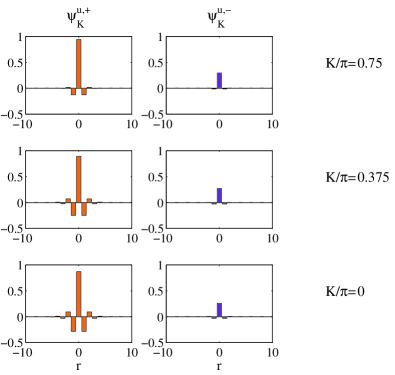
Figure 4: Spinorial components in the $|{\pm}\rangle\,$ channels of the upper bound state for the same parameters of Fig. 3(b), namely $J_{a}=J_{b}=J$, $U_{a}=U_{b}=8J$, $U_{ab}=J$, $\Omega=2.5J$ and the indicated $K$-values.

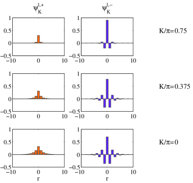
Figure 5: Spinorial components in the $|{\pm}\rangle\,$ channels of the lower bound state for the same parameters of Fig. 3(b), namely $J_{a}=J_{b}=J$, $U_{a}=U_{b}=8J$, $U_{ab}=J$, $\Omega=2.5J$ and the indicated $K$-values.

Once the bound state energies $E^{i}_{BS}$ are determined by solving (20), the bound state wavefunctions $\langle{r}|{\psi^{i}_{K}}\rangle=\sum_{\sigma=\pm}\psi^{i,\sigma}_{K}(r)|{\sigma}\rangle\,$, for $i=u,\,l$, can be obtained by

$$\psi_{K}^{i,\sigma}(r)=G_{K}^{\sigma}(r,0,E^{i}_{BS})\,\sum_{\sigma^{\prime}}U_{\sigma,\sigma^{\prime}}\psi_{K}^{i,\sigma^{\prime}}(0).$$ (21)

The explicit form of the Green’s function written in Eq. (18) implies that the amplitudes in the $|{\pm}\rangle\,$ states have the following spatial dependence

$$\psi^{\sigma}_{K}(r) = \psi^{\sigma}_{K}(0)(\lambda_{K}^{\sigma})^{|r|},$$ (22)

with $\lambda_{K}^{\sigma}$ previously defined in Eq. (III.1). Eventually the ratio at $r=0$ of the spinor components can be written, e.g., as

$$\frac{\psi_{K}^{i,-}(0)}{\psi_{K}^{i,+}(0)}=\frac{2\sqrt{(E^{i}_{BS}(K)-2\Omega)^{2}-\beta_{K}^{2}}}{{\rm sgn}(E^{i}_{BS}(K)-2\Omega)(U-U_{ab})}-\frac{U+U_{ab}}{U-U_{ab}}.\;\;\;\;\;\;\;$$ (23)

From Eq. (22), it appears clearly that the bound states are given by two exponentially localized wavefunctions for the $|{\pm}\rangle\,$ components with different $K$-dependent decay constants , as shown in Figs. 4 and 5 for upper and lower bound state respectively. The sign of $E_{BS}-\Omega_{\sigma}$ determines the sign of $\lambda_{K}^{\sigma}$, which is negative for bound state energies above the $\sigma$-essential spectrum and positive for bound state energies below $\Gamma_{ess}^{\sigma}$. Assuming $U,U_{ab}>0$, the upper bound state is always above both essential spectra, implying negative values for both $\lambda_{K}^{\sigma}$ and a $\pi$-paired oscillating wavefunction typical of repulsively bound pairs winkler2006repulsively . Instead the lower bound state can lie above or between the two essential spectra. In the latter case, $\lambda_{K}^{-}$ is negative, indicating a repulsive character of the bound state in the $|{-}\rangle\,$ internal state, but $\lambda_{K}^{+}$ is positive, indicating that in the $|{+}\rangle\,$ internal state the bound state is actually attractive (see Fig. 5). We remind that the $|{\pm}\rangle\,$ channels describe bound states for two atoms in the rotated internal states $|{a\pm b}\rangle\,$. Therefore the bound state wavefunction shows repulsive or attractive nature, or the co-presence of both, depending on which quantisation direction is chosen in the measurement of the internal state.

$K$-dependent polarization

In the previous part, we have written the bound state wavefunction in terms of the ${|{\pm}\rangle\,}$ states and have shown how the two components depend on the center of mass momentum $K$. The dependence of the internal wavefunction of the dimers on the center of mass momentum $K$ can be referred to, in a broad sense, as a spin-orbit coupling effect.

From the experimental point of view, rather than considering the ${|{\pm}\rangle\,}$ basis, it might be more straighforward to carry out the measurements using the basis $\mathcal{B}_{int}$, already introduced to develop the effective model in Sect. II. The population in the different two-body states $|{2_{a},0_{b}}\rangle\,$, $|{1_{a},1_{b}}\rangle\,$ and $|{0_{a},2_{b}}\rangle\,$ defines a polarization vector $\mathcal{P}^{i}(K)=[\mathcal{P}^{i}_{aa}(K);\mathcal{P}^{i}_{ab}(K);\mathcal{P}^{i}_{bb}(K)]$ for each bound state ($i=u,l$), where obviously $\sum_{\alpha}\mathcal{P}^{i}_{\alpha}=1$.

To quantify the emergent spin-orbit coupling, we look at the $K$-dependence of the polarizazion in the upper bound state. In Fig. 6, we show a typical situation for $|U-U_{ab}|\sim\Omega$ and $U$, $U_{ab}\sim J$. A more detailed analysis, including also the effect of asymmetries between $J_{a},J_{b}$ and $U_{a},U_{b}$ will be presented in Sect. IV.

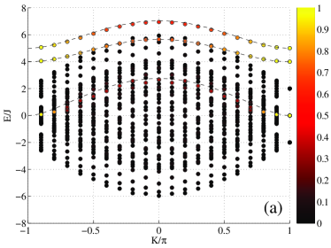
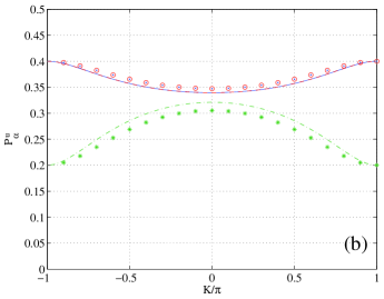
Figure 6: (a) Spectrum as a function of $K$ for $J_{a}=J_{b}=J$, $U_{a}=U_{b}=4J$, $U_{ab}=J$, and $\Omega=J$; the dashed lines are the results of the effective model, while the dots are the eigenenergies of the exact diagonalization; for each eigenstate the population at relative distance $r=0$ is plotted in color scale; in this picture, the dark state spectrum is included for completeness; (b) Polarization ($\mathcal{P}^{u}_{aa}$ (blue full/dots), $\mathcal{P}^{u}_{ab}$ (green dash-dotted/stars), $\mathcal{P}^{u}_{bb}$ (red dashed/circles)) of the upper bound state as a function of $K$. The lines are the results of the effective Hamiltonian and the symbols the results of exact diagonalization.

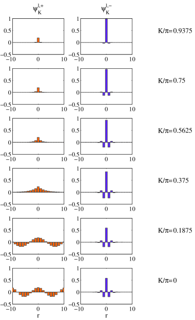
Figure 7: Spinorial components in the $|{\pm}\rangle\,$ channels of the lower bound state for the same parameters of Fig. 3(c), namely $J_{a}=J_{b}=J$, $U_{a}=U_{b}=8J$, $U_{ab}=4J$, $\Omega=2.5J$ and the indicated $K$-values. When the bound state enters the scattering continuum, we select for each value of $K$ the most localized state in the upper continuum (see colorscale in Fig. 3(c)).

III.2 Bound and scattering states hybridization

As we have already mentioned, for repulsive interaction the lower bound state can enter the upper scattering spectrum. In other words, for $U,U_{ab}>0$, there are energies in the scattering spectrum of two atoms in channel $|{+}\rangle\,$ that are immediately close to a pole in the $T$-matrix for two atoms in channel $|{-}\rangle\,$, identified by the condition $1-G_{K}^{-}(0,0,E)(U+U_{ab})/2=0$.

In the $U(1)$ symmetric case $U_{a}=U_{b}=U_{ab}$, the two internal states ${|{\pm}\rangle\,}$ define two independent channels. For each channel, at the energies identified by the poles of the Green’s function, one finds either a scattering or a bound state, like in the single species case. Instead, in the general case of different interaction parameters and in the presence of a coherent coupling between two species, the two atoms can be found in a superposition of scattering and bound states. This intriguing concept will be formalized here below.

The Lippmann-Schwinger equations for $E\in\Gamma^{+}_{ess}$ read

$$\psi_{K}^{+}(r) = \cos(k_{E}r)+G_{K}^{+,s}(r,0,E)\sum_{\sigma^{\prime}}\,U_{\sigma,\sigma^{\prime}}\psi_{K}^{\sigma^{\prime}}(0),$$ (24)

$$\psi_{K}^{-}(r) = G_{K}^{-}(r,0,E)\sum_{\sigma^{\prime}}\,U_{\sigma,\sigma^{\prime}}\psi_{K}^{\sigma^{\prime}}(0),$$ (25)

where we introduced the internal momentum $k_{E}$ satisfying $E=-4J\cos(K/2)\cos(k_{E})+\Omega_{+}$, the Green’s function $G_{K}^{-}$ has been defined in (18) and the bare Green’s function for the scattering states reads

$$G_{K}^{+,s}(r,0,E)=\frac{2}{\beta_{K}}\frac{\sin(k_{E}|r|)}{\sin(k_{E})}.$$ (26)

The components of the spinor wavefunction are therefore

$$\psi_{K}^{+}(r)=\cos(k_{E}r)+$$ (27)

$$G_{K}^{+,s}(r,0,E)\frac{U+U_{ab}}{2}\left[1+\frac{\frac{(U-U_{ab})^{2}}{2(U+U_{ab})}G_{K}^{-}(0,0,E)}{1-G_{K}^{-}(0,0,E)\frac{U+U_{ab}}{2}}\right],$$

$$\psi_{K}^{-}(r)=G_{K}^{-}(r,0,E)\frac{U-U_{ab}}{2}\frac{1}{1-G_{K}^{-}(0,0,E)\frac{U+U_{ab}}{2}}.$$

From the above expressions, it is straightforward to extract some important properties of the hybridised state: first of all, the $\psi_{K}^{+}$ component presents a delocalized wavefunction, typical of scattering states; on the other hand, $\psi_{K}^{-}$ shows a localized exponentially decreasing wavefunction typical of bound states.

Unless $U=U_{ab}$, the two components feel each other and are hybrized. The amplitude of the $\psi_{K}^{-}$ component is amplified, the closer the energy is to the bare bound state energy of two atoms in the two-body state $|{-}\rangle\,$. At the same time the $\psi_{K}^{+}$ component undergoes a phase shift determined by both by the interaction coefficient $(U+U_{ab})/2$ in the ${|{+}\rangle\,}$ channel and the presence of the bound component in the $|{-}\rangle\,$ channel. Eventually, in the strongly interacting limit, where the scattering part strongly dominates over the solution of the homogeneous equation, the wavefunction is fermionized and developes a dip at $r=0$. In the presence of the $\psi_{K}^{-}$ component, the strongly interacting limit is reached close to the pseudo-resonance condition $\sqrt{(E+2\Omega)^{2}-\beta_{K}^{2}}\approx(U+U_{ab})/2$. Those features are reproduced in Fig. 7 where we plot the wavefunction varying $K$ from the Brillouin zone edge towards the center for the parameters corresponding to Fig. 3(c): At the Brillouin zone boundary there exists a purely bound state; around $|K|/\pi\approx 0.3$ the eigenstates become hybridized presenting both bound and scattering characters.

IV Asymmetric case

In this section, we address the most general case where $J_{a}\neq J_{b}$ and $U_{a}\neq U_{b}$ using exact diagonalization and generalizing the effective model. As a basis for exact diagonalization calculations, it is convenient to use all possible distributions in the lattice sites of two bosons in the single particle atomic states $a$ and $b$ . We label all eigenstates with a well-defined value of the center of mass momentum $K$ and determine the spectrum for bound and scattering states. In order to compare the information about the polarization of the system provided by effective Hamiltonian, we should integrate the wavefunction provided by the exact solution over relative distance.

The effective Hamiltonian, written in the basis $\mathcal{B}_{int}$, has the shape shown in Eq. (5) presenting off-diagonal couplings equal to $\sqrt{2}\Omega$, and diagonal elements, which now explicitely read

$$\left\{\begin{split}&E^{a}_{K}=\mbox{sgn}(U_{a})\cdot\sqrt{U_{a}^{2}+16J_{a}^{2}\cos\left(\frac{Kd}{2}\right)^{2}},\\ &E^{ab}_{K}=\mbox{sgn}(U_{ab})\cdot\sqrt{U_{ab}^{2}+16\left(\frac{J_{a}+J_{b}}{2}\right)^{2}\cos\left(\frac{Kd}{2}\right)^{2}+16\left(\frac{J_{a}-J_{b}}{2}\right)^{2}\sin\left(\frac{Kd}{2}\right)^{2}},\\ &E^{b}_{K}=\mbox{sgn}(U_{b})\cdot\sqrt{U_{b}^{2}+16J_{b}^{2}\cos\left(\frac{Kd}{2}\right)^{2}}.\end{split}\right.$$ (28)

The most relevant difference with respect to the symmetric case is that the dark and bright manifolds are not defined anymore and in general three non degenerate bound states are to be expected.

Depending on the specific choice of parameters, the $K$-dependence of the polarization can be strongly enhanced or strongly suppressed. To quantify the amount of spin-orbit coupling present in the system, we define the visibility ${\mathcal{V}}^{u}_{\alpha}=\max_{K}[\mathcal{P}^{u}_{\alpha}]-\min_{K}[\mathcal{P}^{u}_{\alpha}]$ for the different components of the polarization $\mathcal{P}^{u}$.

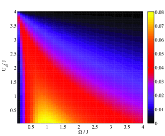
Figure 8: Visibility of $\mathcal{P}^{u}_{aa}$ for $J_{a}=J_{b}=J$, and $U_{a}=U_{b}=4J$ as a function of $\Omega$ and $U_{ab}$. This plot is obtained using the effective model, which proves to be very reliable in a broad range of parameters.

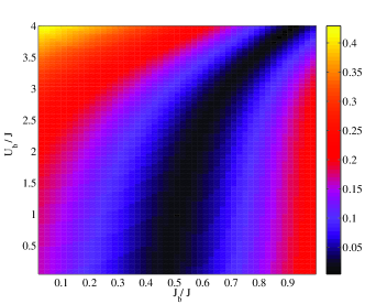
Figure 9: Visibility of $\mathcal{P}^{u}_{aa}$ for $J_{a}=J$, $U_{a}=4J$, $U_{ab}=J$, and $\Omega=J$ as a function of $J_{b}$ and $U_{b}$. This plot is obtained using the effective model, which proves to be very reliable in a broad range of parameters.

We first consider the symmetric case. From Fig. 8, we see that for fixed $U_{a}=U_{b}=U$, $J_{a}=J_{b}$, the visibility of $\mathcal{P}^{u}_{aa}$ is largest when $U-U_{ab}\sim 4\Omega$ and $U-U_{ab}$ largest. The visibility for the other components follows straighforwardly from the relations $\mathcal{P}^{u}_{bb}=\mathcal{P}^{u}_{bb}$ and the normalization condition. Larger values of $U$ produce very similar behaviours but, as expected, an overall smaller amount of coupling between internal and external degrees of freedom.

Taking as a reference the parameters used in Figs. 6, $U_{a}=4J$, $U_{ab}=J$ and $\Omega=J$, which roughly satisfy the above conditions, we study how the visibility is affected when asymmetry between the two species is introduced by varying $J_{b}$ and $U_{b}$. The results for the visibility of $\mathcal{P}^{u}_{aa}$ is shown in Fig. 9. In this case a non trivial dependence is observed, in particular as far as the effect of the different tunneling parameters is concerned.

In general, the effective model produces very reliable results for the energy and polarization of the upper bound state in a broad range of parameters, as one can for instance observe in Fig. 6. This includes the cases where the lowest bound state is actually immersed in the scattering continuum and consequently not well described by the effective model. To get a more precise idea of the regimes of validity of the effective model, we calculated the relative difference of the upper bound state energy and polarization between effective and exact model. At the Brillouin zone edge $K=\pi$ the effective Hamiltonian always produces exact results, since there are no scattering states available to hybridize the bound states. One obtains exact agreement for $\Omega=0$, which is a trivial case, and for $U=U_{ab}$ as expected, due to the restored $U(1)$ symmetry. The agreement is good for $|U-U_{ab}|\ll\Omega$ and $|U|,|U_{ab}|\ll\Omega$, namely the cases where the dominant coherent coupling creates bound states in the coherent $|{\pm}\rangle\,$ superpositions. However, it is important to note that even if in the case of largest spin-orbit coupling, namely $|U-U_{ab}|\sim\Omega$, the error becomes of the order of several percent, the predictions of the effective model remain qualitatively reliable.

V Distinguishable particles

As discussed in the previous sections, the emergent momentum dependent polarisation is a consequence of the competition between breaking of Galilean invariace, coherent coupling and interactions. Therefore, a $K$-dependence of the internal state composition of dressed dimers is quite a general feature, not unique to the previously discussed system. In particular, similar concepts can be applied to the case of two distinguishable particles, as long as at least one of them is characterised by two internal states, namely $a$ and $b$ coupled by an exchange term $\Omega$. Let us called $c$ the state of the second species or isotope atom. Interactions are characterized by the two coefficients $U_{ac}$ and $U_{bc}$. The different terms of the 2-particle Hubbard-like Hamiltonian in Eq. (1) now read

$$\begin{split}&\hat{H}_{kin}=-J_{a}\sum_{\langle i,j\rangle}\hat{a}^{\dagger}_{i}\hat{a}_{j}-J_{b}\sum_{\langle i,j\rangle}\hat{b}^{\dagger}_{i}\hat{b}_{j}-J_{c}\sum_{\langle i,j\rangle}\hat{c}^{\dagger}_{i}\hat{c}_{j},\\ &\hat{H}_{int}=\sum_{i}\left(U_{ac}\hat{n}_{i}^{a}\hat{n}_{i}^{c}+U_{bc}\hat{n}_{i}^{b}\hat{n}_{i}^{c}\right),\\ &\hat{H}_{\Omega}=\sum_{i}\Omega(\hat{a}_{i}^{\dagger}\hat{b}_{i}+\hat{b}_{i}^{\dagger}\hat{a}_{i}),\end{split}$$ (29)

with $\sum_{i}({n}_{i}^{a}+{n}_{i}^{b}+{n}_{i}^{c})=2$. As in Sect. III, the convenient basis is provided by the two-body internal eigenstates of $\hat{H}_{\Omega}$

$$\mathcal{B}_{\Omega}=\left\{\begin{split}&|{+}\rangle\,=\frac{|{1_{a},0_{b},1_{c}}\rangle\,+|{0_{a},1_{b},1_{c}}\rangle\,}{\sqrt{2}},\\ &|{-}\rangle\,=\frac{|{1_{a},0_{b},1_{c}}\rangle\,-|{0_{a},1_{b},1_{c}}\rangle\,}{\sqrt{2}},\end{split}\right.$$ (30)

with eigenvalues $\Omega_{\sigma}=\sigma\Omega$. The eigenstates of the Hamiltonian can be written as spinor wavefunctions $\sum_{\sigma}e^{iKR}\psi^{\sigma}_{K}(r)|{\sigma}\rangle\,$ with $|{\sigma}\rangle\,\in\mathcal{B}_{\Omega}$.

Provided that $J_{a}=J_{b}=J_{c}$, the relative motion for $\psi^{\sigma}_{K}(r)$ is described again by Eq. (14) and interactions are now given by the $2\times 2$ matrix

$$U_{\sigma,\sigma^{\prime}}=\left(\begin{array}[]{cccc}\frac{U_{ac}+U_{bc}}{2}&\frac{U_{ac}-U_{bc}}{2}\\ \frac{U_{ac}-U_{bc}}{2}&\frac{U_{ac}+U_{bc}}{2}\end{array}\right).$$ (31)

The analogy with the case described in detail in Sect. III is striking and similar conclusions can be reached.

Analogously, we can write an effective Hamiltonian under the form

$$\hat{H}_{eff}(K) = \left(\begin{array}[]{cc}E^{ac}_{K}&\Omega\\ \Omega&E^{bc}_{K}\end{array}\right),$$ (34)

where Eq. (3) with $U_{\alpha}=U_{ac},U_{bc}$ provides the diagonal elements. Two different interaction couplings $U_{ac}\neq U_{bc}$ lead to $K$-dependent polarisation for the bound states as previously discussed. From the experimental point of view, considering two distinguishable particles could facilitate the realization of different interaction and hopping strengths.

VI Conclusions and perspectives

In this work we have investigated the bound states of two coherently coupled interacting bosons. We have shown an emerging momentum dependent polarisation due to the non separability of the centre of mass and relative coordinates. We have derived an effective Hamiltonian, which has allowed us to give a direct interpretation of the coherently coupled system in terms of effectively coherently coupled bound states, and tested its validity against exact solutions based on the Lippmann-Schwinger equation and exact diagonalization. We have extended our study to the most general case where different tunneling parameters and interaction strengths for the two internal states are considered, in order to possibly access realistic experimental situations and found the conditions to optimize the correlations between internal and external degrees of freedom. The general character of our results has been stressed by introducing a similar model for two indistinguishable particles where only one needs to be dressed by a Rabi coupling.

On the experimental side, many of the ingredients necessary to study the physics of spin-momentum coupling are already available. Many experiments have been already realised for coherently coupled Bose gas, starting from the seminal investigations in 1999 Cornell99 , to the Josephson and classical bifurcation experiments Zibold2010 ; OberthalerTwin , the realisation of polarisation dependent persistent currents ZoranSC , till the most recent experiments on spin-orbit coupling, artificial gauge fields and synthetic dimensions, where optical lattices are also present (see e.g. DalibardVarenna2014 ). The most difficult issue is the possibility of realising large enough differences between intra- and inter-species interactions. Indeed for the most commonly used ⁸⁷Rb atoms, the difference is very small and Feshbach resonances are difficult to implement. A possible idea would be to consider two different atomic species, as discussed at the end of this work. Alternatively, one could lift the degeneracy of the hyperfine states in, e.g. the $F=1$ manifold and use spin-selective microwave pulses to couple the $F=2$ states in such a way to reduce the intra-species interaction leaving the inter-species unchanged Papoular . Another possibility could be to work with spin-dependent lattices as recently shown in EsslingerSpinLat . In this configuration, aside from breaking $\mathbf{Z}_{2}$ symmetry, by changing the overlap between $a$ and $b$ species one could also sensibly tune the inter-species interaction.

- (1) D. Jaksch and P. Zoller, Annals of physics 315, 52, (2005).
- (2) I. Bloch, J. Dalibard, and W. Zwerger, Rev. Mod. Phys. 80, 885 (2008).
- (3) M. Greiner, O. Mandel, T. Esslinger, T. W. Hänsch, and I. Bloch, Nature 415, 39 (2001).
- (4) M. Lewenstein, A. Sanpera, and V. Ahufinger, Ultracold Atoms in Optical Lattices, International Series of Monographs on Physics (Oxford University Press, 2003)
- (5) S. Baier, M. J. Mark, D. Petter, K. Aikawa, L. Chomaz, Z. Cai, M. Baranov, P. Zoller, and F. Ferlaino, arXiv:1507.03500 [cond-mat.quant-gas].
- (6) J. Simon, W. S. Bakr, R. Ma, M. E. Tai, P. M. Preiss, and M. Greiner, Nature 472, 307 (2011).
- (7) D. Greif, T. Uehlinger, G. Jotzu, L. Tarruell, and T. Esslinger, Science 340, 1307 (2013).
- (8) T. Fukuhara, P. Schauss, M. Endres, S. Hild, M. Cheneau, I. Bloch, and C. Gross, Nature 502, 76 (2013).
- (9) M. Aidelsburger, M. Atala, M. Lohse, J. T. Barreiro, B. Paredes, and I. Bloch, Phys. Rev. Lett. 111, 185301 (2013).
- (10) H. Miyake, G. A. Siviloglou, C. J. Kennedy, W. .C. Burton, and W. Ketterle, Phys. Rev. Lett. 111, 185302 (2013).
- (11) M. Mancini, G. Pagano, G. Cappellini, L. Livi, M. Rider, J. Catani, C. Sias, P. Zoller, M. Inguscio, M. Dalmonte, and L. Fallani, Science, 349, 1510 (2015).
- (12) D. C. Mattis, Rev. Mod. Phys. 58, 361 (1986).
- (13) J. Hubbard, Proceedings of the Royal Society of London, Series A, Mathematical and Physical Sciences, 276, 238 (1963).
- (14) K. Winkler, G. Thalhammer, F. Lang, R. Grimm, J. Hecker Denschlag, A. J. Daley, A. Kantian, H. P. Büchler, and P. Zoller, Nature 441, 853 (2006).
- (15) E. Orignac and T. Giamarchi, Phys. Rev. B 57, 11713 (1998).
- (16) L. Barbiero, M. Abad, and A. Recati, arXiv:1403.4185 [cond-mat.quant-gas].
- (17) F.Zhan, J. Sabbatini, M. J. Davis, and I. P. McCulloch, Phys. Rev. A 90, 023630 (2014).
- (18) M. Valiente and D. Petrosyan, J. Phys. B 41, 161002 (2008).
- (19) M. R. Matthews, B. P. Anderson, P. C. Haljan, D. S. Hall, M. J. Holland, J. E. Williams, C. E. Wieman, and E. A. Cornell, Phys. Rev. Lett. 83, 3358 (1999).
- (20) T. Zibold, E. Nicklas, C. Gross, and M. K. Oberthaler, Phys. Rev. Lett. 105, 204101 (2010).
- (21) C. Gross, H. Strobel, E. Nicklas, T. Zibold, N. Bar-Gill, G. Kurizki, and M. K. Oberthaler, Nature 480, 219 (2011).
- (22) S. Beattie, S. Moulder, R. J. Fletcher, and Z. Hadzibabic, Phys. Rev. Lett. 110, 025301 (2013).
- (23) J. Dalibard, arXiv:1504.05520v1 [cond-mat.quant-gas].
- (24) D. J. Papoular, G. V. Shlyapnikov, and J. Dalibard, Phys. Rev. A 81, 041603(R) (2010).
- (25) G. Jotzu, M. Messer, F. Görg, D. Greif, R. Desbuquois, and T. Esslinger, Phys. Rev. Lett. 115, 073002 (2015).