Gate-tunable zero-frequency current cross-correlations of the quartet mode in a voltage-biased three-terminal Josephson junction

Abstract

A three-terminal Josephson junction biased at opposite voltages can sustain a phase-sensitive dc-current carrying three-body static phase coherence, known as the “quartet current”. We calculate the zero-frequency current noise cross-correlations and answer the question of whether this current is noisy (like a normal current in response to a voltage drop) or noiseless (like an equilibrium supercurrent in response to a phase drop). A quantum dot with a level at energy $\epsilon_{0}$ is connected to three superconductors $S_{a}$, $S_{b}$ and $S_{c}$ with gap $\Delta$, biased at $V_{a}=V$, $V_{b}=-V$ and $V_{c}=0$, and with intermediate contact transparencies. At zero temperature, nonlocal quartets (in the sense of four-fermion correlations) are noiseless at subgap voltage in the nonresonant dot regime $\epsilon_{0}/\Delta\gg 1$, which is demonstrated with a semi-analytical perturbative expansion of the cross-correlations. Noise reveals the absence of granularity of the superflow splitting from $S_{c}$ towards $(S_{a},S_{b})$ in the nonresonant dot regime, in spite of finite voltage. In the resonant dot regime $\epsilon_{0}/\Delta\lesssim 1$, cross-correlations measured in the $(V_{a},V_{b})$ plane should reveal an “anomaly” in the vicinity of the quartet line $V_{a}+V_{b}=0$, related to an additional contribution to the noise, manifesting the phase sensitivity of cross-correlations under the appearance of a three-body phase variable. Phase-dependent effective Fano factors $F_{\varphi}$ are introduced, defined as the ratio between the amplitudes of phase modulations of the noise and the currents. At low bias, the Fano factors $F_{\varphi}$ are of order unity in the resonant dot regime $\epsilon_{0}/\Delta\lesssim 1$, and they are vanishingly small in the nonresonant dot regime $\epsilon_{0}/\Delta\gg 1$.

I Introduction

The Josephson effect and multiple Andreev reflections (MARs) appear to be well established at present time in two-terminal set-ups Averin1 ; Averin2 ; Cuevas ; Cuevas-noise , especially with respect to the clearcut break-junction experimentsSaclay1 ; Saclay2 . Less is known about three terminals. A few recent works Cuevas-Pothier ; Freyn ; Jonckheere ; Francois ; Houzet-Samuelsson ; Duhot ; Riwar ; Padurariu ; Delft dealt with superconducting nanoscale devices with three superconductors $S_{a}$, $S_{b}$ and $S_{c}$ biased at $V_{a}$, $V_{b}$ and $V_{c}=0$, instead of superconducting weak links with only two terminals. It was established by Cuevas and Pothier Cuevas-Pothier on the basis of Usadel equations that the third terminal $S_{c}$ can be viewed qualitatively as having the same effect as an rf-source, producing what was coined Cuevas-Pothier as “self-induced Shapiro steps”. Later, Freyn et al.Freyn rediscovered those voltage resonances, and identified in the adiabatic regime the emergence of intermediate states involving correlations among four, six, eight, … fermions (the so-called quartets, sextets, octets, …). The condition for appearance of a coherent dc-current at a $(p,q)$-resonance is $p(V_{a}-V_{c})+q(V_{b}-V_{c})=0$. Nonlocal quartets correspond to $(p,q)=(1,1)$, nonlocal sextets to $(p,q)=(1,2)$ or $(2,1)$, nonlocal octets to $(p,q)=(1,3)$, $(2,2)$ or $(3,1)$, … For tunnel contacts and at low bias, allowing an adiabatic approximation, the dc-current at a $(p,q)$ resonance is given by

$$I^{c}_{p,q}\sin\left[p\left(\varphi_{a}(t)-\varphi_{c}(t)\right)+q\left(\varphi_{b}(t)-\varphi_{c}(t)\right)\right]$$ (1)

$$= I^{c}_{p,q}\sin\left[p\left(\varphi_{a}(0)-\varphi_{c}(0)\right)+q\left(\varphi_{b}(0)-\varphi_{c}(0)\right)\right],$$

where the last identity is valid only at a $(p,q)$ resonance $p(V_{a}-V_{c})+q(V_{b}-V_{c})=0$ at which the nonlocal Josephson effect becomes time-independent, and the critical current $I^{c}_{p,q}$ can be calculated at equilibrium. It turns out that the microscopic process of four-fermion exchange produces a $\pi$-shifted current-phase relation for the quartets Jonckheere instead of a standard “$0$”-junction. A fully nonequilibrium calculation for the current at voltage resonance was carried out by Jonckheere et al.Jonckheere Correlations among pairs and quasiparticles were also obtained in this work in the form of phase-sensitive MARs (ph-MARs). The recent Grenoble experiment on metallic junctions by Pfeffer et al.Francois provided evidence for phenomena compatible with quartets. However, this experiment could not firmly establish whether the anomaly is due to the quartet mechanism or the oscillations of populations. This question is somehow marginal: both effects can appear simultaneously because of cross-over between those two limiting cases. An more relevant question is that of reconsidering synchronization in a phase-coherent mesoscopic sample.

It is shown here that noise experiments in three-terminal Josephson junctions should provide complementary characterization of those phase-coherent processes, similarly to Cooper pair splitting in three-terminal normal metal-superconductor-normal metal set-ups ref5 ; ref6-7 ; Samuelsson ; ref9 ; Faoro ; Bignon ; Morten ; Melin-Martin ; Freyn-Floser-Melin ; Floser-Feinberg-Melin ; Heiblum ; Takis . A well-understood mechanism for noise in voltage-biased normal-fermionic junctions is partition noise. A well-known intuitive picture envisions a (noiseless) incoming beam of regularly spaced fermionic wave-packets. Each wave-packet incoming on the barrier is transmitted with probability $T$, and reflected with probability $1-T$. The randomness of the transmission process produces noise in the transmitted signal. The noise at arbitrary transmission $T$ is proportional to $T(1-T)$, to the charge of the carriers, and to the voltage.

However, this physical picture for partition noise does not apply to equilibrium superflows of Cooper pairs in response to different phases on different leads (in the absence of applied voltage), because a superflow is collective and nongranular. The calculations presented in the main body of our article are based on a previous article by Cuevas et al.Cuevas-noise , which turned out to be successful in establishing the noise of MARs in a two-terminal set-up. In particular, a dc-Josephson current is noiseless at zero temperature.

Let us come back to three-terminals superconducting junctions, which contain both ingredients of applied voltages and dc-supercurrent of pairs Freyn . Three-body static phase coherence is present in both the pair current (quartets or multipairs) and the quasiparticle current (multiple Andreev reflections, MARs). One expects that noise cross-correlations may help to separate the underlying microscopic processes. A natural question arises in view of the discussion above on the noise of a normal or superconducting flow: Is the phase-sensitive current noiseless or noisy? This question is the subject of the present article.

The notion of “quartets” is now discussed from a different perspective. Focusing on the case $V_{a}-V_{c}=-(V_{b}-V_{c})$, the appearance of a Josephson-like dc-current between, on the one hand, $S_{c}$, and on the other hand the pair ($S_{a},S_{b}$), signals the existence of static phase coherence between the three superconductors, despite the presence of nonzero voltages, in the absence of static phase coherence between two conductors only. The three-body coherence manifests itself in the relevant ”quartet” three-body phase variable $\varphi_{Q}=\varphi_{a}+\varphi_{b}-2\varphi_{c}$, that is in principle controllable with superconducting loops. In general, the dc-current is a periodic function of the variable $\varphi_{Q}$. The latter form suggests that instead of exchanging single Cooper pairs as in a $SNS$ or $SIS$ junction ($I$ is an insulating barrier), the exchange “currency” to establish static phase coherence between $S_{c}$ and ($S_{a},S_{b}$) is an electronic quartet. This macroscopic point of view is valid irrespective of the nature of the junction and of the parameter regime, close or far from equilibrium.

Two distinct pictures for the notion of “quartets” are then envisioned. Notion A corresponds to the restrictive sense of four-fermion correlations, as those appearing in the adiabatic regime Freyn . The (more general) notion B is that of a currency exchanged to establish three-body static phase coherence, characterized by the “quartet phase” $\varphi_{Q}$. It will be shown that the resonant dot regime $\Gamma/\Delta\sim 1$ and $\epsilon_{0}/\Delta\lesssim 1$ leads to finite phase-sensitive noise for the quartets according to B. [The parameter $\epsilon_{0}$ is the quantum dot energy level with respect to the chemical potential of lead $S_{c}$.] By contrast, nonresonant-dot quartets (for $\epsilon_{0}/\Delta\gg 1$) corresponding to A will be shown to be noiseless once the current cross-correlations will be normalized to the currents. A gate voltage can be used to cross-over from the nonresonant ($\epsilon_{0}/\Delta\gg 1$) to the resonant dot ($\epsilon_{0}/\Delta\lesssim 1$) regimes, and thus to control the value of the noise in the quartet mode.

Further technical introductory material is presented in Sec. II. It will be shown in Sec. III on the basis of semi-analytical calculations that the nonresonant-dot quartet current looks like an equilibrium dc-Josephson current in the sense that it is noiseless. Sec. IV demonstrates by numerical calculations that finite noise and noise cross-correlations are produced in the resonant dot regime, depending on the three-body phase variable $\varphi_{Q}$ mentioned above. It will be concluded in Sec. V that an anomaly in the noise or in the noise cross-correlations may be observed in future experiments with resonant quantum dots. Moreover, the anomaly in the noise is predicted to disappear as the quantum dot energy level is made nonresonant by applying a gate voltage, because of a cross-over towards a collective nongranular flow of Cooper pairs in the presence of finite voltages.

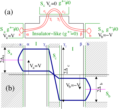
Figure 1: The figure shows a set-up in which three superconductors $S_{a}$, $S_{b}$ and $S_{c}$ biased at $V_{a}=V$, $V_{b}=-V$ and $V_{c}=0$ are connected to a common insulator-like region. Panels a and b correspond respectively to space and energy representations for the butterfly diagram, encoding nonresonant-dot quartets with a current $I_{c}$ though $S_{c}$ set by $I_{c}=I_{c}^{(0)}\sin\varphi_{Q}$, with $\varphi_{Q}=\varphi_{a}+\varphi_{b}-2\varphi_{c}$. On this figure, the central region is equivalent to an insulator-like region, used to address the nonresonant dot regime in Sec. III. However, the numerical calculations in the forthcoming Sec. IV deal with a set-up containing an embedded quantum dot (see Fig. 3).

II Expression of the noise in terms of Keldysh Green’s functions

II.1 Expression of the noise

Three superconducting leads $S_{a}$, $S_{b}$ and $S_{c}$ biased at $V_{a}=V$, $V_{b}=-V$ and $V_{c}=0$ are connected to a common region (insulating or nonresonant quantum dot). The method used here is taken from the papers by Cuevas et al.Cuevas ; Cuevas-noise on the current and noise of a two-terminal superconducting contact (see the Appendix).

The kernel of current-current correlations between terminals $a_{k}$ and $a_{l}$ ($a_{k},a_{l}\in\{S_{a},S_{b},S_{c}\}$) is given by

$$K_{a_{k},a_{l}}(\tau,\tau^{\prime})=\langle\delta I_{a_{k}}(\tau+\tau^{\prime})\delta I_{a_{l}}(\tau)\rangle,$$ (2)

where $\delta I_{a_{k}}(\tau)$ is the current fluctuation of terminal $a_{k}$ at time $\tau$. Because of the explicit time-dependence of the Hamiltonian, the current-current correlations $S_{a_{k},a_{l}}(\tau,\tau^{\prime})$ depend on both times $\tau$ and $\tau^{\prime}$, not only on $\tau-\tau^{\prime}$. The noise correlations are given byCuevas-noise

$$S_{a_{k},a_{l}}(\tau)=\hbar\int d\tau^{\prime}K_{a_{k},a_{l}}(\tau,\tau^{\prime})$$ (3)

The kernel given by Eq. (2) is expressed in terms of the Keldysh Green’s functions $\hat{G}^{+,-}$ and $\hat{G}^{-,+}$, for instance:

$$\hat{K}_{a,b}(\tau,\tau^{\prime})=\frac{e^{2}}{\hbar^{2}}\mbox{Tr}$$ (4)

$$\left\{\hat{\Sigma}_{\beta,b}(\tau)\hat{\tau}_{3}\hat{G}^{+,-}_{b,a}(\tau,\tau^{\prime})\hat{\Sigma}_{a,\alpha}(\tau^{\prime})\hat{\tau}_{3}\hat{G}^{-,+}_{\alpha,\beta}(\tau^{\prime},\tau)\right.$$

$$+ \hat{\Sigma}_{b,\beta}(\tau)\hat{\tau}_{3}\hat{G}^{+,-}_{\beta,\alpha}(\tau,\tau^{\prime})\hat{\Sigma}_{\alpha,a}(\tau^{\prime})\hat{\tau}_{3}\hat{G}^{-,+}_{a,b}(\tau^{\prime},\tau)$$ (5)

$$- \hat{\Sigma}_{\beta,b}(\tau)\hat{\tau}_{3}\hat{G}^{+,-}_{b,\alpha}(\tau,\tau^{\prime})\hat{\Sigma}_{\alpha,a}(\tau^{\prime})\hat{\tau}_{3}\hat{G}^{-,+}_{a,\beta}(\tau^{\prime},\tau)$$ (6)

$$- \hat{\Sigma}_{b,\beta}(\tau)\hat{\tau}_{3}\hat{G}^{+,-}_{\beta,a}(\tau,\tau^{\prime})\hat{\Sigma}_{a,\alpha}(\tau^{\prime})\hat{\tau}_{3}\hat{G}^{-,+}_{\alpha,b}(\tau^{\prime},\tau)$$ (8)

$$\left.+(\tau\leftrightarrow\tau^{\prime})\right\},$$

where the trace “Tr” is a summation over the Nambu labels. Latin labels $a$, $b$, $c$ are used for the tight-binding sites in the superconducting leads, and Greek labels $\alpha$, $\beta$ and $\gamma$ are used for the insulating region. The label $x$ will be used in Sec. IV for a zero-dimensional quantum dot (see also the Appendix). Notations like $\hat{\Sigma}_{a,\alpha}$ or $\hat{\Sigma}_{\alpha,a}$ have the meaning of the hopping amplitude for crossing the interface $S_{a}I$ in the direction $a\rightarrow\alpha$ or $\alpha\rightarrow a$ respectively. The Keldysh Green’s functions in Eqs. (4)-(8) are given by

$$\hat{G}^{+,-}_{i,j}(\tau,\tau^{\prime})=$$

$$i\left(\begin{array}[]{cc}\langle c_{j\uparrow}^{+}(\tau^{\prime})c_{i\uparrow}(\tau)\rangle&\langle c_{j\downarrow}(\tau^{\prime})c_{i\uparrow}(\tau)\rangle\\ \langle c_{j\uparrow}^{+}(\tau^{\prime})c_{i\downarrow}^{+}(\tau)\rangle&\langle c_{j\downarrow}(\tau^{\prime})c_{i\downarrow}^{+}(\tau)\rangle\end{array}\right)$$ (11)

and

$$\hat{G}^{-,+}_{i,j}(\tau,\tau^{\prime})=$$

$$-i\left(\begin{array}[]{cc}\langle c_{i\uparrow}(\tau)c_{j\uparrow}^{+}(\tau^{\prime})\rangle&\langle c_{i\uparrow}(\tau)c_{j\downarrow}(\tau^{\prime})\rangle\\ \langle c_{i\downarrow}^{+}(\tau)c_{j\uparrow}^{+}(\tau^{\prime})\rangle&\langle c_{j\downarrow}^{+}(\tau)c_{j\downarrow}(\tau^{\prime})\rangle\end{array}\right).$$ (14)

The gauge is such that the tunnel terms (purely diagonal in Nambu) are time-dependent:

$$\Sigma_{a_{k},\alpha_{k}}^{1,1}(t) = \Sigma_{a_{k},\alpha_{k}}^{1,1}\exp(iV_{a_{k}}t/\hbar)$$ (15)

$$\Sigma_{a_{k},\alpha_{k}}^{2,2}(t) = \Sigma_{a_{k},\alpha_{k}}^{2,2}\exp(-iV_{a_{k}}t/\hbar),$$ (16)

with $\Sigma_{\alpha_{k},a_{k}}^{1,1}(t)=[\Sigma_{a_{k},\alpha_{k}}^{1,1}(t)]^{*}$, and $\Sigma_{\alpha_{k},a_{k}}^{2,2}(t)=[\Sigma_{a_{k},\alpha_{k}}^{2,2}(t)]^{*}$. The expression for the noise kernel is conveniently Fourier transformed.

II.2 Adiabatic limit

Of particular interest is to show that the noise vanishes in the adiabatic limit. The adiabatic limit corresponds to very small applied voltage, whatever interface transparencies. Then, the phases evolve slowly in time and the Keldysh Green’s functions are approximated as being parameterized by the quasi-static phase variables $\varphi_{a,b,c}$. Fourier transforming from the time difference $\tau-\tau^{\prime}$ to frequency $\omega$ leads to the following expression for the Keldysh Green’s functions:

$$\hat{G}^{+,-}(\omega) = n_{F}(\omega)\left[G^{A}(\omega)-G^{R}(\omega)\right]$$ (17)

$$\hat{G}^{-,+}(\omega) = \left(n_{F}(\omega)-1\right)\left[G^{A}(\omega)-G^{R}(\omega)\right],$$ (18)

where $n_{F}(\omega)$ is the equilibrium Fermi distribution function at zero temperature, and at energy $\omega$. Those expressions are easily deduced from the corresponding Dyson equations for the Keldysh Green’s function, which, in a compact notation, take the following form:

$$\hat{G}^{+,-} = \left(\hat{I}+\hat{G}^{R}\hat{\Sigma}\right)\hat{g}^{+,-}\left(\hat{I}+\hat{\Sigma}\hat{G}^{A}\right)$$ (19)

$$= \left(\hat{I}+\hat{G}^{R}\hat{\Sigma}\right)n_{F}\left(\hat{g}^{A}-\hat{g}^{R}\right)\left(\hat{I}+\hat{\Sigma}\hat{G}^{A}\right)$$ (20)

$$= n_{F}\left(\hat{I}+\hat{G}^{R}\hat{\Sigma}\right)\left(\hat{g}^{A}-\hat{g}^{R}\right)\left(\hat{I}+\hat{\Sigma}\hat{G}^{A}\right)$$ (21)

$$= n_{F}\left\{\left(\hat{I}+\hat{G}^{R}\hat{\Sigma}\right)\hat{G}^{A}-\hat{G}^{R}\left(\hat{I}+\hat{\Sigma}\hat{G}^{A}\right)\right\}$$ (22)

$$= n_{F}\left(G^{A}(\omega)-G^{R}(\omega)\right).$$ (23)

Going from Eq. (20) to Eq. (21), it was used that the voltages are identical in all leads, from what it is deduced that the occupation number $n_{F}\equiv n_{F}(\omega)$ can be factored out. It is noticed that the noise kernel [see Eqs. (4)-(8)] involves products between Eqs. (17) and (18). Again, the Fermi occupation numbers factor out, and the product $n_{F}(\omega)\left(1-n_{F}(\omega)\right)$ is vanishingly small at zero temperature: the current-current (cross-)correlations are vanishingly small in the adiabatic limit.

The next step, considered in the following Sec. III, is to show that the quartet contribution to the noise cross-correlations is vanishingly small in the nonresonant dot limit, for subgap voltages. The nonresonant dot limit corresponds to very low interface transparencies, whatever the applied voltages.

III Strongly nonresonant dot regime

It is supposed in this section on perturbative calculations in transparency that three superconducting leads $S_{a},S_{b}$ and $S_{c}$ are connected to a (small) common insulating region (see Fig. 1). This set-up on Fig. 1 is equivalent to a strongly nonresonant quantum dot (with $\epsilon_{0}/\Delta\gg 1$) embedded in a structure with three superconductors. The strongly nonresonant regime $\epsilon_{0}/\Delta\gg 1$ is addressed here with perturbation theory in the junction transparency. The bare Keldysh Green’s functions denoted by $\hat{g}_{a,a}^{+,-}$, $\hat{g}_{b,b}^{+,-}$ and $\hat{g}_{c,c}^{+,-}$ are finite in the superconducting leads, but the bare Keldysh Green’s function is vanishingly small in the insulator, due to the absence of density of states in this regionCaroli . An expansion of the current and noise in powers of the tunnel amplitudes can be represented schematically by diagrams. Of particular interest here is the “butterfly diagram” for the quartets Freyn , which forms a closed loop in space and in energy (thus leading to a dc-term in the current and noise). The microscopic process of quartets is the lowest order coupling to the three-body phase variable $\varphi_{Q}$ (see Fig. 1). The calculation proceeds by expanding each term contributing to the noise cross-correlations $S_{a,b}$ [see Eqs. (4)-(8)] to order $\Sigma^{8}$ according to the quartet butterfly diagram. In addition, the Nambu labels for electrons and holes are selected in such a way as to produce the correct electron-hole conversions with respect to the quartet butterfly diagram [see Fig. 1b]. For instance the “11” Nambu component of the term (4) is given at order $\Sigma^{8}$ by the following three terms:

$$\hat{\Sigma}_{\beta,b}^{1,1/0,1}\hat{\tau}_{3}^{1,1/1,1}\hat{g}^{+,-/1,2/1,1}_{b,b}\hat{\Sigma}_{b,\beta}^{2,2/1,2}\hat{g}^{A/2,2/2,2}_{\beta,\gamma_{2}}\hat{\Sigma}^{2,2/2,2}_{\gamma_{2},c_{2}}\hat{g}^{A/2,1/2,2}_{c_{2},c_{1}}\hat{\Sigma}^{1,1/2,2}_{c_{1},\gamma_{1}}\hat{g}^{A/1,1/2,2}_{\gamma_{1},\alpha}$$

$$\times\hat{\Sigma}_{\alpha,a}^{1,1/2,1}\hat{g}^{A,1,2/1,1}_{a,a}\hat{\Sigma}^{2,2/1,0}_{a,\alpha}\hat{\tau}_{3}^{2,2/0,0}\hat{g}^{R/2,2/0,0}_{\alpha,\gamma_{1}}\hat{\Sigma}^{2,2/0,0}_{\gamma_{1},c_{1}}\hat{g}^{-,+/2,1/0,0}_{c_{1},c_{2}}\hat{\Sigma}^{1,1/0,0}_{c_{2},\gamma_{2}}\hat{g}^{A/1,1/0,0}_{\gamma_{2},\beta}$$

$$+ \hat{\Sigma}_{\beta,b}^{1,1/0,1}\hat{\tau}_{3}^{1,1/1,1}\hat{g}^{R/1,2/1,1}_{b,b}\hat{\Sigma}_{b,\beta}^{2,2/1,2}\hat{g}^{R/2,2/2,2}_{\beta,\gamma_{2}}\hat{\Sigma}^{2,2/2,2}_{\gamma_{2},c_{2}}\hat{g}^{+,-/2,1/2,2}_{c_{2},c_{1}}\hat{\Sigma}^{1,1/2,2}_{c_{1},\gamma_{1}}\hat{g}^{A/1,1/2,2}_{\gamma_{1},\alpha}$$

$$\times\hat{\Sigma}_{\alpha,a}^{1,1/2,1}\hat{g}^{A/1,2/1,1}_{a,a}\hat{\Sigma}^{2,2/1,0}_{a,\alpha}\hat{\tau}_{3}^{2,2/0,0}\hat{g}^{R/2,2/0,0}_{\alpha,\gamma_{1}}\hat{\Sigma}^{2,2/0,0}_{\gamma_{1},c_{1}}\hat{g}^{-,+/2,1/0,0}_{c_{1},c_{2}}\hat{\Sigma}^{1,1/0,0}_{c_{2},\gamma_{2}}\hat{g}^{A/1,1/0,0}_{\gamma_{2},\beta}$$

$$+ \hat{\Sigma}_{\beta,b}^{1,1/0,1}\hat{\tau}_{3}^{1,1/1,1}\hat{g}^{R/1,2/1,1}_{b,b}\hat{\Sigma}_{b,\beta}^{2,2/1,2}\hat{g}^{R/2,2/2,2}_{\beta,\gamma_{2}}\hat{\Sigma}^{2,2/2,2}_{\gamma_{2},c_{2}}\hat{g}^{R/2,1/2,2}_{c_{2},c_{1}}\hat{\Sigma}^{1,1/2,2}_{c_{1},\gamma_{1}}\hat{g}^{R/1,1/2,2}_{\gamma_{1},\alpha}$$

$$\times\hat{\Sigma}_{\alpha,a}^{1,1/2,1}\hat{g}^{+,-,1,2/1,1}_{a,a}\hat{\Sigma}^{2,2/1,0}_{a,\alpha}\hat{\tau}_{3}^{2,2/0,0}\hat{g}^{R/2,2/0,0}_{\alpha,\gamma_{1}}\hat{\Sigma}^{2,2/0,0}_{\gamma_{1},c_{1}}\hat{g}^{-,+/2,1/0,0}_{c_{1},c_{2}}\hat{\Sigma}^{1,1/0,0}_{c_{2},\gamma_{2}}\hat{g}^{A/1,1/0,0}_{\gamma_{2},\beta},$$

and similar expressions are obtained for all of the $28$ terms contributing to the current-current cross-correlations [see Eqs. (4)-(8)]. Expressions like $\hat{\Sigma}_{a,\alpha}^{\tau_{1},\tau_{2}/n_{1},n_{2}}$ have the meaning of traversing the interface $S_{a}I$ upon changing the Nambu labels according to $\tau_{1}\rightarrow\tau_{2}$, and the labels of harmonics according to $n_{1}\rightarrow n_{2}$. The hopping amplitudes do not change the value $\tau_{2}=\tau_{1}$ of the Nambu labels, but they increment by $n_{2}=n_{1}\pm 1$ the label of harmonics. On the contrary, the anomalous bare Green’s function changes the value of the Nambu labels, but the labels of harmonics are left unchanged because of the choice of the gauge.

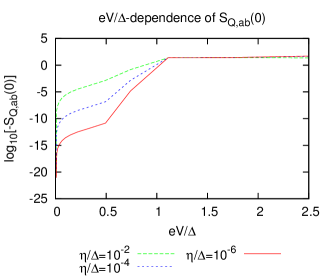
Figure 2: Voltage dependence of the quartet contribution to the current-current cross-correlations, for the values of $\eta/\Delta$ shown on the figure. The parameter $\eta$ is a regulator introduced as the imaginary part of the energy $\omega$.

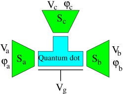
Figure 3: Schematics of a quantum dot connected to three superconductors $S_{a}$, $S_{b}$ and $S_{c}$ at voltages $V_{a}$, $V_{b}$ and $V_{c}$. A gate voltage $V_{g}$ is applied to the quantum dot.

It is first shown that our expansion in the tunnel amplitude $\Sigma$ is compatible with the vanishingly small value of the noise in the adiabatic limit (see Sec. II). For this purpose, we collected the only four terms at order $\Sigma^{8}$ containing only advanced or only retarded Green’s functions, but no products between the former and the latter. It is indeed those terms that encode the adiabatic limit, because the current in this limit is expressed as the sum or difference of terms that contain only advanced or only retarded Green’s functions [see the form of the Keldysh Green’s function in Eq. (23)]. Once those terms are identified, it is easy to show for the harmonics labels that the Green’s functions $\hat{g}^{+,-}_{a,a}$ and $\hat{g}^{+,-}_{b,b}$ contain identical sets of harmonics labels, meaning that those terms do not contribute to the noise at zero temperature, because of a prefactor of the type $n_{F}(\omega+p\omega_{0}/2)[n_{F}(\omega+p\omega_{0}/2)-1]$, where $p$ is an integer. The contribution of those “adiabatic” terms to the noise is thus vanishingly small, in agreement with the discussion of the adiabatic limit in Sec. II.2.

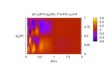
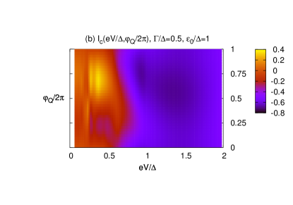
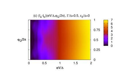
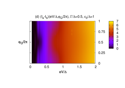
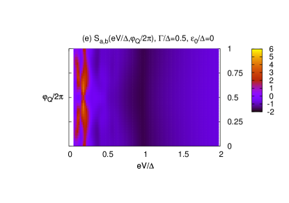
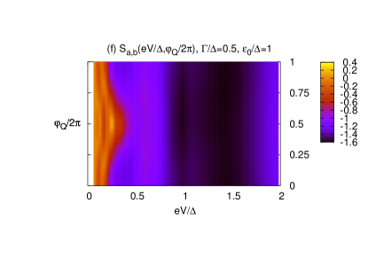
Figure 4: Color-map in the $(eV/\Delta,\varphi_{Q}/2\pi)$ plane of the multipair current $I_{c}$ (panels a, b), of the current difference $I_{a}-I_{b}$ (panels c, d), and of the current cross-correlations $S_{a,b}$ (panels e, f). The current is in units of $e\Delta/h$ and the current cross-correlations are un units of $e^{2}\Delta/h$. The contact transparencies are such that $\Gamma/\Delta=0.5$. Panels a, c and e correspond to $\epsilon_{0}/\Delta=0$, and panels b, d, f to, $\epsilon_{0}/\Delta=1$.

Now, numerical results are presented for the perturbative calculation in transparency, in which the $28$ lowest-order terms in the quartet contribution to the zero-frequency cross-correlations $S_{Q,ab}(0)$ are evaluated numerically at zero phase. The voltage dependence of $S_{Q,ab}(0)$ is shown (in log scale) in Fig. 2, for different values of $\eta/\Delta$ over four orders of magnitude. The small parameter $\eta\ll\Delta$ corresponds to a line-width broadening introduced as the imaginary part to the energy, and intended to regularize perturbation theory. If $eV/\Delta>1$, the $\varphi_{Q}=0$ cross-correlations are negative and large in absolute value, due to the fact that, in this voltage range, extended electron-like states below the gap of $S_{a}$ are coupled by the quartets to extended hole-like states above the gap of $S_{b}$. As $eV/\Delta$ is reduced below unity, much smaller values of $S_{Q,ab}$ are obtained, because $S_{Q,ab}$ is due to the residual density of states inside the superconducting gap. Shoulders appear in the voltage-dependence of the cross-correlations, due to the gap edge singularities. Extrapolating to $\eta/\Delta\rightarrow 0^{+}$ leads to the conclusion that nonresonant-dot quartets do not contribute to the current-current cross-correlations at subgap voltage.

IV Quantum dot-superconductor three-terminal Josephson junction

A few results are known for the current-current cross correlations in a three-terminal all-superconducting structure with arbitrary interface transparencies. Phase-insensitive positive cross-correlations were discovered by Duhot, Lefloch and Houzet Duhot in the incoherent regime. The phase-sensitive thermal noise and noise cross-correlations of a superconducting structure at equilibrium was calculated by Freyn et al.Freyn with the Hamiltonian approach. Very recently, Riwar et al.Riwar-noise provided a fully nonperturbative calculation of the noise of a three-terminal Josephson junction biased at equal voltages. In what follows, the junction is biased at opposite voltages, therefore allowing for the emergence of a nonstandard quartet mode, not present for equal voltages.

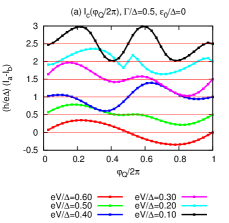
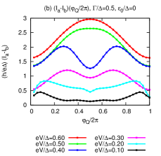
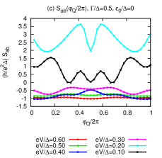
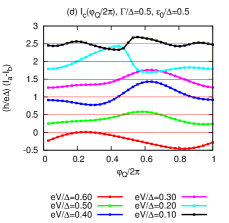
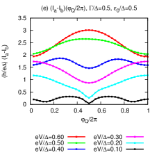
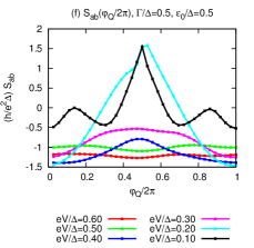
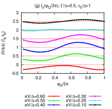
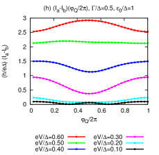
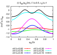
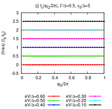
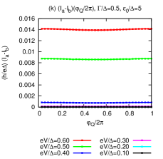
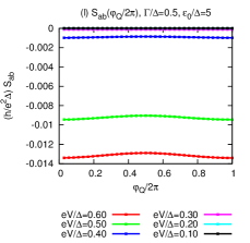
Figure 5: The figure shows the sensitivity on the phase $\varphi_{Q}$ of $I_{c}$ (panels a, d, g and j), $I_{a}-I_{b}$ (panel b, e, h and k) and $S_{a,b}$ (panels c, f, i and l), for the voltages indicated on the figure. For clarity, the data on panel a, d, g and j were shifted along $y$ axis according to the solid red lines. No shift is applied to the other panels.

It is first recalled that a quantum dot is connected to three superconducting leads $S_{a}$, $S_{b}$ and $S_{c}$ biased at opposite voltages $V_{a}=-V_{b}\equiv V$, and $V_{c}=0$ respectively. The normal-state transparency of the contacts is controlled by $\Gamma=t^{2}/W$, where $t$ is the hopping amplitude between the dot and the superconductors in their normal state, and $W$ is the hopping term in the bulk of the superconductors (a fraction of the bandwidth). It is supposed now that a single energy level is within the superconducting gap window, and, in addition, this energy level $\epsilon_{0}$ (controllable by a gate voltage) is varied systematically, thus allowing to cross-over from nonresonant-dot quartets (for $\epsilon_{0}/\Delta\gg 1$) to resonant-dot quartets for $\epsilon_{0}/\Delta\lesssim 1$, with different behavior of the noise in both regimes.

It was established by Jonckheere et al.Jonckheere that the current has two components: with particle-hole symmetry, the current $I_{c}$ (due to multipairs generalizing quartets) is even in voltage and odd in the phase $\varphi_{Q}$, and the current difference $I_{a}-I_{b}$ (due to ph-MARs) is odd in voltage and even in the phase $\varphi_{Q}$. Fig. 4 shows how $I_{c}$, the current difference $I_{a}-I_{b}$ and the cross-correlations $S_{a,b}$ vary in the parameter plane $(eV/\Delta,{\varphi_{Q}}/2\pi)$, for the experimentally relevant intermediate $\Gamma/\Delta=0.5$. The current and noise exhibit a dependence on the three-body phase variable $\varphi_{Q}=\varphi_{a}+\varphi_{b}-2\varphi_{c}$. Panels a, c, e and b, d, f of Fig. 4 correspond respectively to $\epsilon_{0}/\Delta=0$ and $\epsilon_{0}/\Delta=1$, thus in the resonant dot regime. The values of the current and noise cross-correlations are large in the resonant dot regime $\epsilon_{0}/\Delta\lesssim 1$, which contrasts with the nonresonant dot regime $\epsilon_{0}/\Delta\gg 1$ (see the preceding Sec. III). The current $I_{c}$, the current difference $I_{a}-I_{b}$ and the cross-correlations $S_{a,b}$ have a strong dependence on the quartet phase $\varphi_{Q}$ in the nonresonant dot regime $\epsilon_{0}/\Delta\lesssim 1$. A weak dependence on $\varphi_{Q}$ of those quantities was obtained numerically for $\epsilon_{0}/\Delta=5$ (not shown in Fig. 4), in a qualitative agreement with Sec. III.

The current-current cross-correlations $S_{a,b}$ are shown by a color-plot in Fig. 4e and Fig. 4f in the plane of the variables $(eV/\Delta,\varphi_{Q}/2\pi)$, for the same values $\epsilon_{0}/\Delta=0$ (panel e) and $\epsilon_{0}/\Delta=1$ (panel f). Positive and phase-sensitive current-current cross-correlations resonances emerge below $eV/\Delta\lesssim 0.4$. An experiment measuring cross-correlations in the $(V_{a},V_{b})$ plane should thus detect an additional contribution to the cross-correlations if the three-body phase variable $\varphi_{Q}$ becomes a relevant quantity at the quartet resonance $V_{a}+V_{b}=0$ (with $V_{c}=0$).

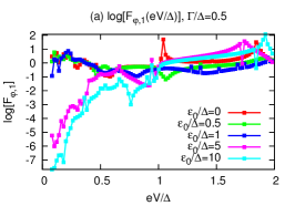
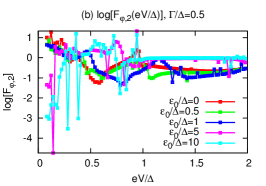
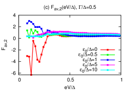
Figure 6: The figure shows the sensitivity on normalized voltage $eV/\Delta$ of the logarithm of the phase Fano factors $F_{\varphi,1}=\delta S_{a,b}/\delta(I_{c})$ (panel a) and $F_{\varphi,2}=\delta S_{a,b}/\delta(I_{a}-I_{b})$ (panel b), where the symbol $\delta X$ has the meaning of $\delta X=\mbox{Max}_{\varphi_{Q}}X(\varphi_{Q})-\mbox{Min}_{\varphi_{Q}}X(\varphi_{Q})$. Panel c shows the $eV/\Delta$-dependence of the average Fano factor $F_{av,2}=S_{a,b,av}/I_{c,av}$, where the subscript “av” denotes averaging over the phase $\varphi_{c}$.

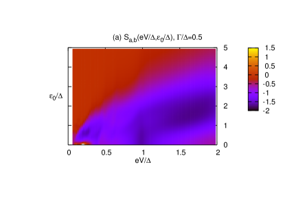
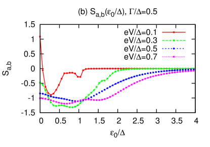
Figure 7: Current-current cross-correlations $S_{a,b}(eV/\Delta,\epsilon_{0}/\Delta)$ for $\Gamma/\Delta=0.5$ (panel a). The cross-correlations become negligible in the nonresonant dot regime $\epsilon_{0}/\Delta\gtrsim\epsilon_{0}^{*}/\Delta$. The value of $\epsilon_{0}^{*}/\Delta$ decreases to zero as $eV/\Delta$ is reduced. Panel b shows the current-current cross-correlations $S_{a,b}(\epsilon_{0}/\Delta)$ for $\Gamma/\Delta=0.5$, and for the values $eV/\Delta=0.1,0.3,0.5,0.7$.

The color-plots in Fig. 4 for $I_{c}$, $I_{a}-I_{b}$ and $S_{a,b}$ are complemented by conventional one-parameter plots (see Fig. 5) which better illustrate the phase sensitivity of the currents and current-current cross-correlations. Let us first consider the multipair current (Fig. 5 a, d, g, j), which is, as expected, odd in the phase $\varphi_{Q}$. A strongly anharmonic behavior is clearly obtained for $\epsilon_{0}/\Delta\lesssim 1$ and $eV/\Delta\ll 1$, with a quasi-period doubling as $eV/\Delta$ is reduced from $eV/\Delta=0.6$ to $eV/\Delta=0.1$ if $\epsilon_{0}/\Delta=0$ (Fig. 5 a), pointing towards emerging octets at low bias. Quasi-harmonic and “$0$”-junction behaviors are recovered for vanishingly small $\epsilon_{0}/\Delta=0$ and larger $eV/\Delta$. In contrast, for larger $\epsilon_{0}/\Delta$, an harmonic behavior is obtained with a “$\pi$”-junction character. Second, the quasiparticle current $I_{a}-I_{b}$ is, as expected, even in phase, and, contrarily to $I_{c}$, it has a nonzero phase-averaged value (Fig. 5 b, e, h, k). The latter represents the “usual” phase-insensitive MARs, which increases with $eV/\Delta$. On the other hand, the phase modulation represents the phase-MARs and it also displays anharmonic behavior at small voltage. Third, the panels c, f, i and l of Fig. 5 represent the cross-correlations $S_{a,b}(\varphi_{Q})$. As a new result, one finds that, like the quasiparticle current, it is even in phase, and it has a nonzero phase average. An especially complex harmonic content is obtained on panel c. A general trend is that negative current-current cross-correlations are obtained for $\epsilon_{0}/\Delta=5$, which become negligibly small as the voltage is reduced below $eV/\Delta\lesssim 0.3$ (see Fig. 5l). This behavior is consistent with the absence of current-current cross-correlations for the nonresonant-dot quartets at low bias voltage (see Sec. III). Positive current-current cross-correlations emerge gradually as $\epsilon_{0}/\Delta$ is reduced, first for the lowest bias voltage $eV/\Delta=0.1$ in a specific window of the phase variable $\varphi_{Q}$ if $\epsilon_{0}/\Delta=1$ (see Fig. 5i). Positive current-current cross-correlations are obtained for the lowest value $\epsilon_{0}/\Delta=0$ (see Fig. 5c), at low normalized bias voltage $eV/\Delta=0.1\div 0.2$ and in the full range of $\varphi_{Q}$.

A closer look at panels a-l of Fig. 5 reveals that the current-current cross-correlations correlate weakly with the multipair current $I_{c}$, but the correlation is better with the current difference $I_{a}-I_{b}$ (corresponding to the physical process of ph-MARs). One notices that “kinks” emerge in $S_{a,b}$ at $\varphi_{c}=\pi/2$ for $\epsilon_{0}/\Delta=0.5$ and $eV/\Delta=0.1$, $0.2$ (see Fig. 5f). Those kinks in the cross-correlations are to be put in correspondence with similar features in $I_{a}-I_{b}$ (ph-MARs, see Fig. 5e), not present in $I_{c}$ (multipair current, see Fig. 5d). The same analogy between $S_{a,b}$ and $I_{a}-I_{b}$ is also visible for $\epsilon_{0}/\Delta=0$ (see Figs. 5a, b and c).

It is relevant both experimentally and theoretically to compare the values of the cross-correlations to the values of the currents. It was found previously (see Fig. 4) that the cross-correlations become very small in the nonresonant dot regime $\epsilon_{0}/\Delta\gg 1$ and in the limit of low bias voltage $eV/\Delta\ll 1$. However, the phase-sensitive current is also reduced if $\epsilon_{0}/\Delta\gg 1$, and the question arises of comparing the noise to the current in the nonresonant dot regime at low bias voltage. The quantity $\delta S_{a,b}$ is defined as the difference between the maximum and the minimum (over the phase $\varphi_{Q}$) of $S_{a,b}(\varphi_{Q})$, and a similar definition holds for $\delta I_{c}$ and $\delta[I_{a}-I_{b}]$. A first Fano factor is defined as $F_{\varphi,1}=\delta S_{a,b}/\delta I_{c}$, which is the value of the amplitude of the oscillations of the cross-correlations normalized to the amplitude of the oscillations of the multipair current $I_{c}$. [The symbol $\delta X=\mbox{Max}_{\varphi_{Q}}X(\varphi_{Q})-\mbox{Min}_{\varphi_{Q}}X(\varphi_{Q})$ has the meaning of an amplitude phase variations.] The second Fano factor is defined as the amplitude of the oscillations of the cross-correlations normalized to that of the phase-MAR processes: $F_{\varphi,2}=\delta S_{a,b}/\delta[I_{a}-I_{b}]$. The voltage dependence of $\log(F_{\varphi,1})$ and $\log(F_{\varphi,2})$ are shown in Figs. 6a and b respectively. The different curves on each of those panels correspond to the values $\epsilon_{0}/\Delta=0$, $0.5$, $1$, $5$ and $10$. The spikes on panel b correspond to values of the voltage for which the integral over energy $\omega$ of the current is very small, therefore deteriorating the accuracy in the Fano factor $F_{\varphi,2}$. Indeed, it turns out that, for specific voltages, the amplitudes of oscillations in $I_{a}-I_{b}$ can become very small, because the difference $I_{a}-I_{b}$ goes to zero in the zero-voltage limit. The data-points shown on panels a and b of Fig. 6 correspond to unsmoothed raw data that are however sufficient for the purpose of discussing now the general trends. If $\epsilon_{0}/\Delta=5$, $10$, the Fano factors $F_{\varphi,1}$ and $F_{\varphi,2}$ decrease drastically towards zero as $eV/\Delta$ is reduced. If $\epsilon_{0}/\Delta=0$, $0.5$, $1$ the Fano factors $F_{\varphi,1}$ and $F_{\varphi,2}$ take much higher values of order $0.1\div 1$. In addition, the Fano factor for the noise and current averaged over the phases $F_{av,2}=S_{a,b,av}/[I_{a,av}-I_{b,av}]$ is shown on panel c of Fig. 6, which also demonstrates a strong reduction of $|F_{av,2}|$ at low bias in the nonresonant dot regime. [The symbol $X_{av}=\int X(\varphi_{Q})d\varphi_{Q}/2\pi$ has the meaning of an average over $\varphi_{Q}$.] In addition, a nontrivial change of sign is obtained in $F_{av,2}$, which reflect the overall sign of $S_{a,b}$ (see Fig. 4, Fig. 5 and the forthcoming Fig. 7b).

The results presented in Fig. 6 demonstrate that, at low bias voltage, the cross-correlations $S_{a,b}$ tend to zero faster than the currents in the strongly nonresonant dot regime $\epsilon_{0}/\Delta\gg 1$. The cross-correlations $S_{a,b}$ (in units of the currents) thus become very small in the nonresonant dot regime, but not in the resonant dot regime, suggesting that a gate voltage can be used to monitor the value of cross-correlations at the quartet resonance $V_{a}+V_{b}=0$.

The crossover between the resonant and nonresonant dot regimes is better visualized in Fig. 7a and b. Fig. 7a shows in color-scale the value of the cross-correlations in the plane $(eV/\Delta,\epsilon_{0}/\Delta)$, for $\Gamma/\Delta=0.5$ and $\varphi_{Q}=0$. The red area in the top-left corner of Fig. 7a corresponds to the nonresonant dot regime in which the cross-correlations are very small. The blue area corresponds to large negative cross-correlations. The positive cross-correlations are restricted to the bottom-left corner, as seen from panel b showing the current-current cross-correlations as a function of $\epsilon_{0}/\Delta$ for different values of $eV/\Delta$. At fixed $eV/\Delta$, there is thus a cross-over value $\epsilon_{0}^{*}/\Delta$ of the parameter $\epsilon_{0}/\Delta$ above which the cross-correlations are weak. The value of $\epsilon_{0}^{*}/\Delta$ is strongly reduced as the normalized voltage $eV/\Delta$ is reduced, which appears to be compatible with the absence of current-current cross-correlations in the adiabatic limit (see Sec. II.2).

V Conclusions

To conclude, it is a relevant question to ask whether splitting a supercurrent by quartets at resonant voltages produces positive cross-correlations at zero temperature. Splitting a supercurrent at equilibrium or in the adiabatic limit does not produce noise, and our numerical calculations are consistent with this limit of low bias voltage. It was shown by a semi-analytical perturbative calculation in interface transparency that the quartets are noiseless also in the nonresonant dot regime in the limit of small interface transparencies, for arbitrary voltage below the gap. Those perturbative calculations in interface transparency took the full Keldysh structure into account. However, phase-sensitive positive current-current cross-correlations are obtained numerically in the resonant dot case. A quantum dot was connected to three superconductors with an intermediate coupling $\Gamma/\Delta=0.5$. The resonant dot regime was obtained if the quantum dot energy level $\epsilon_{0}$ is such that $\epsilon_{0}/\Delta\ll 1$ and the nonresonant dot regime corresponds to $\epsilon_{0}/\Delta\gg 1$. These phase-sensitive current cross-correlations correlate in a qualitative manner with the signal of phase-sensitive MARs, which suggests a strong contribution from the latter. Those phase-sensitive MARs correspond to the transmission of a quasiparticle assisted by quartets or by multipairs. In this respect, a nonzero value for the phase-sensitive component of current cross-correlations in noise experiments would imply that quartets or multipairs are present together with quasiparticles. One can conclude that a cross-correlation experiment should detect a gate-tunable anomaly at the quartet resonance $V_{a}+V_{b}=0$. A strong phase-sensitivity of the cross-correlations is predicted in the resonant dot regime $\epsilon_{0}/\Delta\lesssim 1$, and an absence of noise cross-correlations is obtained in the nonresonant dot regime $\epsilon_{0}/\Delta\gg 1$. In an experiment, the width in voltage $(V_{a},V_{b})$ parameter plane of the anomaly obtained for $\epsilon_{0}/\Delta\lesssim 1$ in the cross-correlations is expected to correlate to the Josephson anomaly in the average current, because both anomalies originate from the appearance of the three-body phase variable $\varphi_{Q}=\varphi_{a}+\varphi_{b}-2\varphi_{c}$. It is noted finally that phase-sensitive noise was already calculated and measured in Andreev interferometers Nazarov ; Heikkila . It is proposed here to go one step further and measure an anomaly in the noise or in the cross-correlations of a three-terminal Josephson junction.

Recursive Green’s functions in energy for three-terminal structures

This Appendix generalizes to three terminals the algorithm proposed by Cuevas, Martín Rodero and Levy Yeyati Cuevas ; Cuevas-noise in which the current of MARs was evaluated in a two-terminals structure. All numerical calculations for the three-terminal junction were realized on the basis of of this method.

The Green’s functions $\hat{G}_{n,m}(\omega)$ depend on one energy $\omega$ and two integers $n$ and $m$ (the harmonics of half the Josephson frequency). The Dyson equation takes the form

$$\hat{G}_{n,m} = \hat{K}_{n,n}\hat{G}_{n,m}+\hat{K}_{m,m}^{(0)}\delta_{n,m}+\hat{K}_{n,n+2}\hat{G}_{n+2,m}$$

$$+ \hat{K}_{n,n-2}\hat{G}_{n-2,m},$$

where the dependence on $\omega$ is made implicit. The matrices $K$ have three component, one for each of the terminals:

$$\hat{K}^{n,n}_{(a)} = \left(\begin{array}[]{cc}g_{x,x}^{1,1/n,n}\Sigma_{x,a}^{1,1/n,n+1}g_{a,a}^{1,1/n+1,n+1}\Sigma_{a,x}^{1,1/n+1,n}&0\\ 0&g_{x,x}^{2,2/n,n}\Sigma_{x,a}^{2,2/n,n-1}g_{a,a}^{2,2/n-1,n-1}\Sigma_{a,x}^{2,2/n-1,n}\end{array}\right)$$ (30)

$$\hat{K}^{n,n+2}_{(a)} = \left(\begin{array}[]{cc}0&g_{x,x}^{1,1/n,n}\Sigma_{x,a}^{1,1/n,n+1}g_{a,a}^{1,2/n+1,n+1}\Sigma_{a,x}^{2,2/n+1,n+2}\\ 0&0\end{array}\right)$$ (33)

$$\hat{K}^{n,n-2}_{(a)} = \left(\begin{array}[]{cc}0&0\\ g_{x,x}^{2,2/n,n}\Sigma_{x,a}^{2,2/n,n-1}g_{a,a}^{2,1/n-1,n-1}\Sigma_{a,x}^{2,2/n-1,n-2}&0\end{array}\right).$$ (36)

Similar expressions are obtained for $K_{(b)}$

$$\hat{K}^{n,n}_{(b)} = \left(\begin{array}[]{cc}g_{x,x}^{1,1/n,n}\Sigma_{x,b}^{1,1/n,n-1}g_{b,b}^{1,1/n-1,n-1}\Sigma_{b,x}^{1,1/n-1,n}&0\\ 0&g_{x,x}^{2,2/n,n}\Sigma_{x,b}^{2,2/n,n+1}g_{b,b}^{2,2/n+1,n+1}\Sigma_{b,x}^{2,2/n+1,n}\end{array}\right)$$ (39)

$$\hat{K}^{n,n-2}_{(b)} = \left(\begin{array}[]{cc}0&g_{x,x}^{1,1/n,n}\Sigma_{x,b}^{1,1/n,n-1}g_{b,b}^{1,2/n-1,n-1}\Sigma_{b,x}^{2,2/n-1,n-2}\\ 0&0\end{array}\right)$$ (42)

$$\hat{K}^{n,n+2}_{(b)} = \left(\begin{array}[]{cc}0&0\\ g_{x,x}^{2,2/n,n}\Sigma_{x,b}^{2,2/n,n+1}g_{b,b}^{2,1/n+1,n+1}\Sigma_{b,x}^{2,2/n+1,n+2}&0\end{array}\right).$$ (45)

and for $K_{(c)}$:

$$\hat{K}^{n,n}_{(c)} = \left(\begin{array}[]{cc}g_{x,x}^{1,1/n,n}\Sigma_{x,c}^{1,1/n,n}g_{c,c}^{1,1/n,n}\Sigma_{c,x}^{1,1/n,n}&g_{x,x}^{1,1/n,n}\Sigma_{x,c}^{1,1/n,n}g_{c,c}^{1,2/n,n}\Sigma_{c,x}^{2,2/n,n}\\ g_{x,x}^{2,2/n,n}\Sigma_{x,c}^{2,2/n,n}g_{c,c}^{2,1/n,n}\Sigma_{c,x}^{1,1/n,n}&g_{x,x}^{2,2/n,n}\Sigma_{x,c}^{2,2/n,n}g_{c,c}^{2,2/n,n}\Sigma_{c,x}^{2,2/n,n}\end{array}\right)$$ (48)

$$\hat{K}_{(c)}^{n,n+2} = K_{(c)}^{n,n-2}=0$$ (49)

The matrix $\hat{K}^{(0)}$ is as follows:

$$\hat{K}^{(0)m,m}=\left(\begin{array}[]{cc}g_{x,x}^{1,1/m,m}&0\\ 0&g_{x,x}^{2,2/m,m}\end{array}\right).$$ (52)

Next, Eq. (Recursive Green’s functions in energy for three-terminal structures) is solved by recursion: $\hat{G}_{n-2,m}=\hat{z}^{-}_{n-2,m}\hat{G}_{n,m}$ leads to

$$\hat{z}^{-}_{n,n+2}=\left(\hat{I}-\hat{K}_{n,n}-\hat{K}_{n,n-2}\hat{z}^{-}_{n-2,n}\right)^{-1}\hat{K}_{n,n+2}$$ (53)

for $n<m$. On the other hand, $\hat{G}_{n,m}=z^{+}_{n,n-2}\hat{G}_{n-2,m}$ leads to

$$\hat{z}^{+}_{n,n-2}=\left(\hat{I}-\hat{K}_{n,n}-\hat{K}_{n,n+2}\hat{z}^{-}_{n+2,n}\right)^{-1}\hat{K}_{n,n-2}$$ (54)

if $n>m$. For $n=m$, we find

$$\hat{G}_{m,m}=\left(\hat{I}-\hat{K}_{m,m}-\hat{K}_{m,m+2}\hat{z}^{+}_{m+2,m}-\hat{K}_{m,m-2}\hat{z}^{-}_{m-2,m}\right)^{-1}\hat{K}^{(0)}_{m,m}.$$ (55)

References

- (1) D. Averin and A. Bardas, Phys. Rev. Lett. 75, 1831 (1995).
- (2) D. Averin and H. T. Imam, Phys. Rev. Lett. 76, 3814 (1996).
- (3) J. C. Cuevas, A. Martín-Rodero, and A. Levy Yeyati, Phys. Rev. B54, 7366 (1996).
- (4) J.C. Cuevas, A. Martin-Rodero and A. Levy Yeyati, Phys. Rev. Lett. 82, 4086 (1999).
- (5) E. Scheer, P. Joyez, D. Esteve, C. Urbina, and M. H. Devoret Phys. Rev. Lett. 78, 3535 (1997); E. Scheer, N. Agrait, J. C. Cuevas, A. Levy Yeyati, B. Ludoph, A. Martin-Rodero, G. Rubio Bollinger, J.M. van Ruitenbeek and C. Urbina, Nature 394, 154 (1998).
- (6) R. Cron, M.F. Goffman, D. Esteve and C. Urbina, Phys. Rev. Lett. 86, 4104 (2001).
- (7) J. C. Cuevas and H. Pothier, Phys. Rev. B 75, 174513 (2007).
- (8) A. Freyn, B. Doucot, D. Feinberg, and R. Mélin, Phys. Rev. Lett. 106, 257005 (2011).
- (9) T. Jonckheere, J. Rech, T. Martín, B. Douçot, D. Feinberg, R. Mélin, Phys. Rev. B 87, 214501 (2013).
- (10) S. Duhot, F. Lefloch and M. Houzet, Phys. Rev. Lett. 102, 086804 (2009).
- (11) M. Houzet and P. Samuelsson, Phys. Rev. B 82, 06051 (2010).
- (12) R.-P. Riwar, M. Houzet, J.S. Meyer, Y.V. Nazarov, arXiv:1503.06862.
- (13) B. van Heck, S. Mi, and A.R. Akhmerov, Phys. Rev. B 90, 155450 (2014).
- (14) C. Padurariu, T. Jonckheere, J. Rech, R. Mélin, D. Feinberg, T. Martin, Yu. V. Nazarov, Phys. Rev. B92, 205409 (2015).
- (15) A.H. Pfeffer, J.E. Duvauchelle, H. Courtois, R. Mélin, D. Feinberg, F. Lefloch, Phys. Rev. B 90, 075401 (2014).
- (16) M.P. Anatram and S. Datta, Phys. Rev. B 53, 16390 (1996).
- (17) T. Martin, Phys. Lett. A 220, 137 (1996); J. Torrès and T. Martin, Eur. Phys. J. B 12, 319 (1999).
- (18) P. Samuelsson and M. Büttiker, Phys. Rev. Lett. 89, 046601 (2002); Phys. Rev. B 66, 201306(R) (2002); P. Samuelsson, E.V. Sukhorukov and M. Büttiker, Phys. Rev. Lett. 91, 157002 (2003).
- (19) J. Börlin, W. Belzig and C. Bruder, Phys. Rev. Lett. 88, 197001 (2002).
- (20) L. Faoro, F. Taddei and R. Fazio, Phys. Rev. B 69, 125326 (2004).
- (21) G. Bignon, M. Houzet, F. Pistolesi and F.W.J. Hekking, Europhys. Lett. 67, 110 (2004).
- (22) J.P. Morten, A. Brataas and W. Belzig, Phys. Rev. B 74, 214510 (2006); J.P. Morten, D. Huertas-Hernando, A. Brataas and W. Belzig, Europhys. Lett. 81, 40002 (2008); J.P. Morten, D. Huertas-Hernando, W. Belzig and A. Brataas, Phys. Rev. B 78, 224515 (2008).
- (23) R. Mélin, C. Benjamin, and T. Martin, Phys. Rev. B 77, 094512 (2008).
- (24) A. Freyn, M. Flöser and R. Mélin, Phys. Rev. B 82, 014510 (2010).
- (25) M. Flöser, D. Feinberg and R. Mélin, Phys. Rev. B 88, 094517 (2013).
- (26) L. Hofstetter, S. Csonka, J. Nygård, and C. Schönenberger, Nature 461, 960 (2009); L. G. Herrmann, F. Portier, P. Roche, A. Levy Yeyati, T. Kontos, and C. Strunk, Phys. Rev. Lett. 104, 026801 (2010); L. Hofstetter, S. Csonka, A. Baumgartner, G. Fülöp, S. d’Hollosy, J. Nygård, and C. Schönenberger, Phys. Rev. Lett. 107, 136801 (2011).
- (27) A. Dass, Y. Ronen, M. Heiblum, D. Mahalu, A.V. Kretinin and H. Shtrikman, Nat. Comm. 3, 1165 (2012).
- (28) C. Caroli, R. Combescot, P. Nozières, and D. Saint-James, J. Phys. C 4, 916 (1971); 5, 21 (1972).
- (29) R.-P. Riwar, D. Badiane, M. Houzet, J. Meyer and Y.V. Nazarov, Physica E76, 231 (2016).
- (30) B. Reulet, A.A. Kozhevnikov, D.E. Prober, W. Belzig, and Yu.V. Nazarov, Phys. Rev. Lett. 90, 066601 (2003).
- (31) M.P.V. Stenberg, P. Virtanen, and T.T. Heikkilä, Phys. Rev. B 76, 144504 (2007).