Typical sumsets of linear codes

Abstract

Given two identical linear codes $\mathcal{C}$ over $\mathbb{F}_{q}$ of length $n$, we independently pick one codeword from each codebook uniformly at random. A sumset is formed by adding these two codewords entry-wise as integer vectors and a sumset is called typical, if the sum falls inside this set with high probability. We ask the question: how large is the typical sumset for most codes? In this paper we characterize the asymptotic size of such typical sumset. We show that when the rate $R$ of the linear code is below a certain threshold $D$, the typical sumset size is roughly $|\mathcal{C}|^{2}=2^{2nR}$ for most codes while when $R$ is above this threshold, most codes have a typical sumset whose size is roughly $|\mathcal{C}|\cdot 2^{nD}=2^{n(R+D)}$ due to the linear structure of the codes. The threshold $D$ depends solely on the alphabet size $q$ and takes value in $[1/2,\log\sqrt{e})$. More generally, we completely characterize the asymptotic size of typical sumsets of two nested linear codes $\mathcal{C}_{1},\mathcal{C}_{2}$ with different rates. As an application of the result, we study the communication problem where the integer sum of two codewords is to be decoded through a general two-user multiple-access channel.

I Introduction

Structured codes (linear codes for example) not only permits simple encoding and decoding algorithms, but also provides good interference mitigation properties which are crucial for multi-user communication networks. Specialized to Gaussian wireless networks, lattice codes, which can be seen as linear codes (which are the most well-understood structured codes) lifted to Euclidean space [1], have been studied extensively. Early results on lattice codes including [2] [3] [4] have shown that good (nested) lattice codes are able to achieve the capacity of point-to-point Gaussian channels. Lattice codes are also applied to Gaussian networks, for example the Gaussian two-way relay channel ([5][6]), and yield best known communication rates that cannot be achieved otherwise. More recently, the compute-and-forward [7] framework employs nested lattice codes in a general Gaussian wireless network. It exploits the additivity of the network by addressing the problem of decoding sums of lattice codewords at intermediate nodes in the network. Furthermore nested linear codes (see [8], [9] for example), which can be seen as a generalization of nested lattice codes, are applicable to general multi-user networks other than Gaussian networks.

Consider applying the simplest structured codes — linear codes, to a standard two-user Gaussian multiple access channel (MAC) of the form $Y=X_{1}+X_{2}+Z$. Existing coding schemes using structured codes usually consider two codewords $T_{1}^{n},T_{2}^{n}$ in some vector space over a finite field, say $\mathbb{F}_{q}^{n}$, and require the entry-wise modulo sum $T_{1}^{n}\oplus T_{2}^{n}$ to be decoded at the receiver. But for the Gaussian MAC it is more natural to study the “integer sum” $T_{1}^{n}+T_{2}^{n}$, where two codewords are treated as integer-valued vectors. This is because after lifting linear codes from the $\mathbb{F}_{q}^{n}$ to $\mathbb{R}^{n}$, the additive Gaussian channel sums up $T_{1}^{n},T_{2}^{n}$ as vectors of real numbers instead of in a finite field. The modulo sum $T_{1}^{n}\oplus T_{2}^{n}$ is easy to understand: if $T_{1}^{n},T_{2}^{n}$ are uniformly chosen from a linear code, the sum $T_{1}^{n}\oplus T_{2}^{n}$ stays in that linear code and is still uniformly distributed. But the analysis of the integer sum $T_{1}^{n}+T_{2}^{n}$ is more complicated and its behavior have not been studied.

To put our study in perspective, it is worth pointing out that our problem is closely connected to sumset theory, which studies the size of the set $\mathcal{A}+\mathcal{B}:=\{a+b:a\in\mathcal{A},b\in\mathcal{B}\}$ where $\mathcal{A},\mathcal{B}$ are two finite sets taking values in some additive group. One objective of the sumset theory is to use sumset inequalities to relate the cardinality of sets $|\mathcal{A}|,|\mathcal{B}|$ and $|\mathcal{A}+\mathcal{B}|$. As a simple example, for $\mathcal{A}=\{0,1,2,3,4\}$ with $5$ elements we have $|\mathcal{A}+\mathcal{A}|=9$ elements. But if let $\mathcal{A}^{\prime}=\{0,0.2,0.8,1.1,2.1\}$ with $5$ elements we have $|\mathcal{A}^{\prime}+\mathcal{A}^{\prime}|=15$ elements. This shows that the sumset size $|\mathcal{A}+\mathcal{B}|$ depends heavily on structures of the sets. As a rule of thumb, the sumset size will be small if and only if the individual sets are “structured”. Some classical results of sumset theory and inverse sumset theory can be found in, e.g. [10].

Our problem concerns with sums of random variables defined over a certain set, hence can be viewed as a sumset problem in a probabilistic setting. It shares similarity with the classical sumset problem while has its own feature. We first point out the main difference between the two problems. Given a set of integers $\mathcal{U}=\{0,1,\ldots,q-1\}$, the sumset $\mathcal{U}+\mathcal{U}$ contains $2q-1$ elements. Now let $U_{1},U_{2}$ be two independent random variables uniformly distributed in the set $\mathcal{U}$, a natural connection between the size of the set $\mathcal{U}$ and the random variables $U_{1},U_{2}$ is that $H(U_{1})=H(U_{2})=\log|\mathcal{U}|$, i.e., the entropy of the random variable is equal to the logarithmic size of $\mathcal{U}$. Now we turn to the sum variable $W:=U_{1}+U_{2}$. Although $W$ takes all possible values in $\mathcal{U}+\mathcal{U}$, it is “smaller” than $\log|\mathcal{U}+\mathcal{U}|$ because the distribution of $W$ is non-uniform over $\mathcal{U}+\mathcal{U}$. Indeed we have $H(W)<\log|\mathcal{U}+\mathcal{U}|$ in this case but the difference between $H(W)$ and $\log|\mathcal{U}+\mathcal{U}|$ is small. However this phenomenon is much more pronounced in high dimensional spaces as we shall see later in this paper. On the other hand it is also important to realize that in the probabilistic setting, the structure of the random variable still has decisive impact on the sumset “size”, which can be partially characterized by the entropy of the sum variable. Using the examples in the preceding paragraph, if the identical independent random variables $U_{1},U_{2}$ are uniformly distributed in $\mathcal{A}$, we have $H(U_{1}+U_{2})\approx 2.99$ bit while if $U^{\prime}_{1},U^{\prime}_{2}$ uniformly distributed in $\mathcal{A}^{\prime}$, it gives $H(U^{\prime}_{1}+U^{\prime}_{2})\approx 3.84$ bit. We also point out that the sumset theory for Shannon entropy has been studied recently in e.g. [11] [12] and fundamental results relating $H(X)$ and $H(X_{1}+X_{2})$ are established. However our specific problem about linear codes in high-dimensional spaces requires separate analysis which is not present in the existing literature.

In this paper, we consider two linear codes $\mathcal{C}_{1},\mathcal{C}_{2}$ with rates $R_{1},R_{2}$ while satisfying the condition $\mathcal{C}_{1}\subseteq\mathcal{C}_{2}$ or $\mathcal{C}_{2}\subseteq\mathcal{C}_{1}$. Let $T_{1}^{n},T_{2}^{n}$ be two codewords uniformly chosen from $\mathcal{C}_{1},\mathcal{C}_{2}$ and we would like to understand what does the sum $W^{n}:=T_{1}^{n}+T_{2}^{n}$ look like in $\mathbb{Z}^{n}$ for very large $n$. We will show that when the dimension $n$ goes to infinity, most sums $T_{1}^{n}+T_{2}^{n}$ will fall into a subset $\mathcal{K}$, which could be substantially smaller than the sumset $\mathcal{C}_{1}+\mathcal{C}_{2}$. We characterize the asymptotic size of $\mathcal{K}$ completely and show certain thresholds effects of the size $|\mathcal{K}|$ depending on the values of $R_{1},R_{2}$. We also established the exact relationship between the $H(T_{1}^{n},H_{2}^{n})$ and $H(T_{1}^{n}+T_{2}^{n})$ in the limit and show that the difference between $H(T_{1}^{n}+T_{2}^{n})$ and $\log|\mathcal{C}_{1}+\mathcal{C}_{2}|$ can increase unboundedly as the codewod length $n$ increases. As an application of the results, we study the problem of decoding the integer sum of codewords through a general two-user Gaussian MAC when two users are equipped with two linear codes.

II Typical sumsets of linear codes

In this section we formally define and study typical sumsets of linear codes.

II-A Preliminaries and notations

We use $[a:b]$ to denote the set of integers $\{a,a+1,\ldots,b-1,b\}$ and define two sets $\mathcal{U}:=[0:q-1]$ and $\mathcal{W}:=[0:2q-2]$. We also define $P_{U}$ to be the uniform probability distribution over the set $\mathcal{U}$ i.e.,

$$P_{U}(a)=1/q\mbox{ for all }a\in\mathcal{U}.$$ (1)

If $U_{1},U_{2}$ are two independent random variables with distribution $P_{U}$, the sum $W:=U_{1}+U_{2}$ is a random variable distributed over the set $\mathcal{W}$. Let $P_{W}$ denote the probability distribution of this random variable. A direct calculation shows that

$$P_{W}(a)=\begin{cases}\frac{a+1}{q^{2}}&a\in[0:q-1]\\ \frac{2q-1-a}{q^{2}}&a\in[q:2q-2]\end{cases}$$ (2)

and the entropy of $W$ is given as

$$H(W)=2\log q-\frac{1}{q^{2}}(2\sum_{i=1}^{q}i\log i-q\log q).$$ (3)

Given a probability distribution $P_{U}$ over the alphabet $\mathcal{U}$, we use $\mathcal{A}_{[U]}^{(n)}$ to denote the set of typical sequences defined as:

$$\mathcal{A}_{[U]}^{(n)}:=\left\{{\bf m}:\left|P_{U}(a)-\frac{1}{n}N(a|{\bf m})\right|\leq\delta,\mbox{ for all }a\in\mathcal{U}\right\}$$ (4)

where $N(a|{\bf m})$ is the occurrence count of the symbol $a$ in sequence ${\bf m}=({\bf m}_{1},\ldots,{\bf m}_{n})$. In the paper we will always choose $\delta$ small but satisfying $n\delta^{2}\rightarrow\infty$ as $n\rightarrow\infty$. Similarly we can define the conditional typical sequences $\mathcal{A}_{[Z|U]}^{(n)}({\bf u})$ as well as the typical sequences $\mathcal{A}_{[ZU]}^{(n)}$ determined by a joint distribution $P_{ZU}$ as in [13, Ch. 2]. We recall the standard results regarding the typical sequences.

Lemma 1 (Typical sequences [13])

Let $U^{n}$ be a $n$-length random vector with each entry i.i.d. according to $P_{U}$. Then for every $\delta>0$ in (4), it holds that

$$\mathbb{P}\left\{U^{n}\in\mathcal{A}_{[U]}^{(n)}\right\}\geq 1-2|\mathcal{U}|e^{-2n\delta^{2}}$$ (5)

Furthermore, the size of set of typical sequences is bounded as

$$2^{n(H(U)-\epsilon_{n})}\leq|\mathcal{A}_{[U]}^{(n)}|\leq 2^{n(H(U)+\epsilon_{n})}$$ (6)

for some $\epsilon_{n}\searrow 0$ as $n\rightarrow\infty$.

In this paper vectors and matrices are denoted using bold letters such as ${\bf a}$ and ${\bf A}$, respectively. The $i$-th entry of a vector ${\bf a}$ is denoted as ${\bf a}_{i}$ and ${\bf A}_{i}$ denotes the $i$-th column of the matrix ${\bf A}$. Throughout the paper, the notations ${\bf A}{\bf b}$ or ${\bf a}^{T}{\bf b}$ are understood as matrix multiplication modulo $q$, or the matrix multiplication over the corresponding finite field. Modulo addition is denoted with $\oplus$ and $+$ means the usual addition over integers. Logarithm $\log$ is with base $2$. Sets are usually denoted using calligraphic letters such as $\mathcal{A}$ and their cardinality are denoted by $|\mathcal{A}|$. We often deal with quantities depending on the codeword length $n$. The notation $o_{n}(1)$ denotes a quantity that approaches $0$ as $n\rightarrow\infty$. We say $a\doteq 2^{nb}$ for some constant $b$ if there exists some $\epsilon_{n}\searrow 0$ such that $2^{n(b-\epsilon_{n})}\leq a\leq 2^{n(b+\epsilon_{n})}$. We also consider the probability of events in the limit when the codeword length $n$ goes to infinity. For any event $H$, we say the event $H$ occurs asymptotically almost surely (a.a.s.) if $\mathbb{P}\left\{H\right\}\rightarrow 1$ as $n\rightarrow\infty$.

II-B Problem statement and main results

Given two positive integers $k,n$ satisfying $k<n$, an $(n,k)$-linear code over $\mathbb{F}_{q}$ is a $k$-dimensional subspace in $\mathbb{F}_{q}^{n}$ where $q$ is a prime number. The rate of this code is given by $R:=\frac{k}{n}\log q$. Any $(n,k)$-linear code can be constructed as

$$\mathcal{C}=\left\{{\bf t}:{\bf t}={\bf G}{\bf m},\mbox{ for all }{\bf m}\in\mathbb{F}_{q}^{k}\right\}$$ (7)

with a generator matrix ${\bf G}\in\mathbb{F}_{q}^{n\times k}$ and ${\bf m}$ can be thought as a message. An $(n,k)$-linear code $\mathcal{C}$ over $\mathbb{F}_{q}$ is called systematic if it can be constructed as

$$\mathcal{C}=\left\{{\bf t}:{\bf t}=\begin{bmatrix}{\bf I}_{k\times k}\\ {\bf Q}\end{bmatrix}{\bf m},\mbox{ for all }{\bf m}\in\mathbb{F}_{q}^{k}\right\}$$ (8)

with some ${\bf Q}\in\mathbb{F}_{q}^{(n-k)\times k}$ where ${\bf I}_{k\times k}$ is the $k\times k$ identity matrix.

We are interested in the sumset of two codebooks. More precisely, let $k_{2}\leq k_{1}\leq n$ and use ${\bf m}\in\mathbb{F}_{q}^{k_{1}}$, ${\bf n}^{\prime}\in\mathbb{F}_{q}^{k_{2}}$ to denote two different messages. We concatenate the messages of the codebook with the smaller rate as ${\bf n}:=[^{{\bf n}^{\prime}}_{\bf 0}]$ where ${\bf 0}$ is a zero vector of length $k_{1}-k_{2}$. Two codebooks are generated as

$$\mathcal{C}_{1} :=\left\{{\bf t}:{\bf t}={\bf G}{\bf m},\mbox{ for all }{\bf m}\in\mathbb{F}_{q}^{k_{1}}\right\}$$ (9a)

$$\mathcal{C}_{2} :=\left\{{\bf v}:{\bf v}={\bf G}{\bf n}={\bf G}\begin{bmatrix}{\bf n}^{\prime}\\ {\bf 0}\end{bmatrix},\mbox{ for all }{\bf n}^{\prime}\in\mathbb{F}_{q}^{k_{2}}\right\}$$ (9b)

with some matrix ${\bf G}\in\mathbb{F}_{q}^{n\times k_{1}}$. Since the two codebooks are generated with the common generator matrix ${\bf G}$, we have $\mathcal{C}_{2}\subseteq\mathcal{C}_{1}$ and these two codebooks are called nested. The rates of these two codebooks are $R_{1}:=\frac{k_{1}}{n}\log q,R_{2}:=\frac{k_{2}}{n}\log q$, respectively.

From now on we will view $\mathcal{C}_{1},\mathcal{C}_{2}$ as sets of $n$-length integer-valued vectors taking values in $\mathcal{U}^{n}$ where $\mathcal{U}:=\{0,\ldots,q-1\}$. The sumset of two linear codes is defined as

$$\mathcal{C}_{1}+\mathcal{C}_{2}:=\{{\bf t}+{\bf v}:{\bf t}\in\mathcal{C}_{1},{\bf v}\in C_{2}\}$$ (10)

where the addition is understood as the addition in $\mathbb{Z}$ and is performed element-wise between the two $n$-length vectors. Hence each element in $\mathcal{C}_{1}+\mathcal{C}_{2}$ takes value in $\mathcal{W}^{n}$ where $\mathcal{W}:=\{0,\ldots,2q-2\}$. Let $T_{1}^{n},T_{2}^{n}$ denote two random variables taking values in the code $\mathcal{C}_{1},\mathcal{C}_{2}$ with uniform distribution, i.e.

$$\mathbb{P}\left\{T_{1}^{n}={\bf t}\right\} =q^{-k_{1}}\mbox{ for all }{\bf t}\in\mathcal{C}_{1}$$ (11a)

$$\mathbb{P}\left\{T_{2}^{n}={\bf v}\right\} =q^{-k_{2}}\mbox{ for all }{\bf v}\in\mathcal{C}_{2}$$ (11b)

The sum codewords $T_{1}^{n}+T_{2}^{n}$ is also a random vectors taking values in $\mathcal{C}_{1}+\mathcal{C}_{2}$. There is a natural distribution on $\mathcal{C}_{1}+\mathcal{C}_{2}$ induced by $T_{1}^{n},T_{2}^{n}$, which is formally defined as follows.

Definition 1 (Induced distribution on $\mathcal{C}_{1}+\mathcal{C}_{2}$)

Given two codebooks $\mathcal{C}_{1},\mathcal{C}_{2}$ and assume $T_{1}^{n},T_{2}^{n}$ are two uniformly distributed vectors defined as in (11). We use $P_{\mathcal{S}}$ to denote the distribution on $\mathcal{C}_{1}+\mathcal{C}_{2}$ which is induced from the distribution of $T_{1}^{n},T_{2}^{n}$.

The object of interest in this paper is given in the following definition.

Definition 2 (Typical sumset)

Let $\mathcal{C}_{j}^{(n)},j=1,2$ be a sequence of linear codes indexed by their dimension. Let $T_{1}^{n},T_{2}^{n}$ be two independent random variables uniformly distributed in $\mathcal{C}_{1}^{(n)},\mathcal{C}_{2}^{(n)}$ as in (11). A sequence of subsets $\mathcal{K}^{(n)}\subseteq\mathcal{C}_{1}^{(n)}+\mathcal{C}_{2}^{(n)}$ is called typical sumsets of $\mathcal{C}_{1}^{(n)}$, $\mathcal{C}_{2}^{(n)}$, if $T_{1}^{n}+T_{2}^{n}\in\mathcal{K}^{(n)}$ asymptotically almost surely, i.e., $\mathbb{P}\left\{T_{1}^{n}+T_{2}^{n}\in\mathcal{K}^{(n)}\right\}\rightarrow 1$ as $n\rightarrow\infty$.

To make notations easier, we sometimes often drop the dimension $n$ and say $\mathcal{K}$ is a typical sumset of $\mathcal{C}_{1}$, $\mathcal{C}_{2}$, with the understanding that a sequence of codes are considered as in Definition 2. Clearly the sumset $\mathcal{C}_{1}+\mathcal{C}_{2}$ is always a typical sumset according to the definition because all possible $T_{1}^{n}+T_{2}^{n}$ must fall inside it. However we will show that for almost all linear codes, most sum codewords $T_{1}^{n}+T_{2}^{n}$ will fall into a subset $\mathcal{K}$ which could be much smaller than $\mathcal{C}_{1}+\mathcal{C}_{2}$ by taking the probability distribution of $T_{1}^{n}$ and $T_{2}^{n}$ into account. In fact, we will consider a more general case when one codebook is (possibly) shifted to a coset by a fixed vector. Assume $\mathcal{C}_{1}$ is shifted to $\mathcal{C}_{1}^{\prime}$ with any fixed vector ${\bf d}$ as

$$\mathcal{C}_{1}^{\prime}=\mathcal{C}_{1}\oplus{\bf d}:=\{{\bf t}\oplus{\bf d}:{\bf t}\in\mathcal{C}_{1}\},$$ (12)

the following theorem states the main result in this section.

Theorem 1 (Normal typical sumsets)

Let $\mathcal{C}_{1}^{(n)},\mathcal{C}_{2}^{(n)}$ be two sequences of linear codes in $\mathbb{F}_{q}^{n}$ indexed by their dimension with rate $R_{j}:=\lim_{n\rightarrow\infty}\frac{1}{n}\log|\mathcal{C}_{j}|,j=1,2$. For any fixed vector ${\bf d}\in\mathbb{F}_{q}^{n}$ we define $\mathcal{C}_{1}^{\prime(n)}:=\mathcal{C}_{1}^{(n)}\oplus{\bf d}$ as in (12). Consider the case when $\mathcal{C}_{1}^{(n)},\mathcal{C}_{2}^{(n)}$ are generated as in (9) with the same generator matrix ${\bf G}$ and assume without loss of generality that $\mathcal{C}_{2}^{(n)}\subseteq\mathcal{C}_{1}^{(n)}$. If each entry of the generator matrix ${\bf G}$ is independent and identically chosen according to the uniform distribution $P_{U}$, then asymptotically almost surely there exists a sequence of typical sumsets $\mathcal{K}_{N}^{(n)}\subseteq\mathcal{C}_{1}^{\prime(n)}+\mathcal{C}_{2}^{(n)}$ whose sizes satisfy

$$|\mathcal{K}_{N}^{(n)}| \doteq\min\left\{2^{n(R_{1}+R_{2})},2^{n\left(\max\{R_{1},R_{2}\}+D(q)\right)}\right\}$$ (13)

$$D(q) :=H(U_{1}+U_{2})-\log q$$ (14)

where $U_{1},U_{2}$ are independent random variables with the uniform distribution $P_{U}$ in (1). Furthermore for all ${\bf w}\in\mathcal{K}_{N}^{(n)}$, the induced distribution $P_{\mathcal{S}}$ defined in Definition 1 satisfies

$$P_{\mathcal{S}}({\bf w})\doteq\max\left\{2^{-n(R_{1}+R_{2})},2^{-n\left(\max\{R_{1},R_{2}\}+D(q)\right)}\right\}.$$ (15)

where $P_{\mathcal{S}}$ is the induced probability distribution on $\mathcal{C}_{1}^{\prime(n)}+\mathcal{C}_{2}^{(n)}$.

Proof:

A proof of the theorem is given in Section III. In Appendix A we show that $D(q)$ is an increasing function of $q$ and

$$1/2\leq D(q)<\log\sqrt{e}\approx 0.7213$$ (16)

where the lower bound holds for $q=2$ and the upper bound is approached with $q\rightarrow\infty$. ∎

Remark 1

We point out that there exist linear codes which possess (exponentially) smaller or larger typical sumsets than $\mathcal{K}_{N}$ in (13). For example $|\mathcal{C}_{1}+\mathcal{C}_{2}|$ is always larger or equal to $|\mathcal{K}_{N}|$ and we will give an example of a smaller typical sumset in Section III, Remark 2. To distinguish the specific typical sumset $\mathcal{K}_{N}$ in Theorem 1 from other possible typical sumsets, we will call $\mathcal{K}_{N}$ a normal typical sumset. Theorem 1 shows that randomly generated linear codes a.a.s. have a normal typical sumset $\mathcal{K}_{N}$.

To help us visualize the rather complicated expression in (13), Figure 1 depicts the size of the typical sumset $\mathcal{K}_{N}$. It is also instructive to see how the typical sumset size grows if we fix the rate of one codebook and vary the rate of the other. In Figure 2 we fix $R_{1}$ and plot the size of the normal typical sumset for different $R_{2}$. Depending on the range of $R_{1}$, there are two cases where we have different behaviors of the typical sumset size as $R_{2}$ increases. It is worthy to point out the “saturation” behavior on the size of the typical sumsets. For example let $R_{1}$ be its maximal value $\log q$ and increase $R_{2}$ from $0$ to $\log q$, the typical sumset size increases until $R_{2}$ reaches $D(q)$, but stays unchanged afterwards. It means for $R_{1}=\log q$ and $R_{2}=D(q)$, all possible sum codewords have already appeared in the typical sumset, and adding more codewords to $\mathcal{C}_{2}$ will not create new sum codewords in the typical sumset.

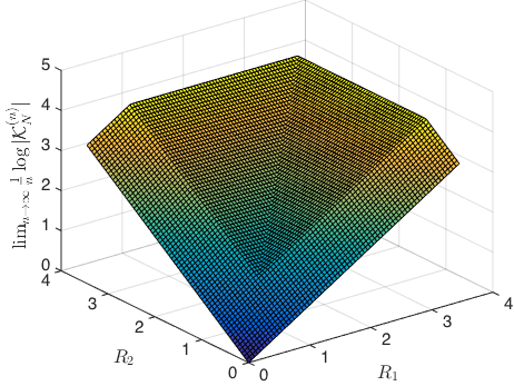
Figure 1: The asymptotic size of the typical sumset $\lim_{n\rightarrow\infty}\frac{1}{n}\log|\mathcal{K}_{N}|$ in (13) as a function of $R_{1},R_{2}$ (In this plot we set $q=11$).

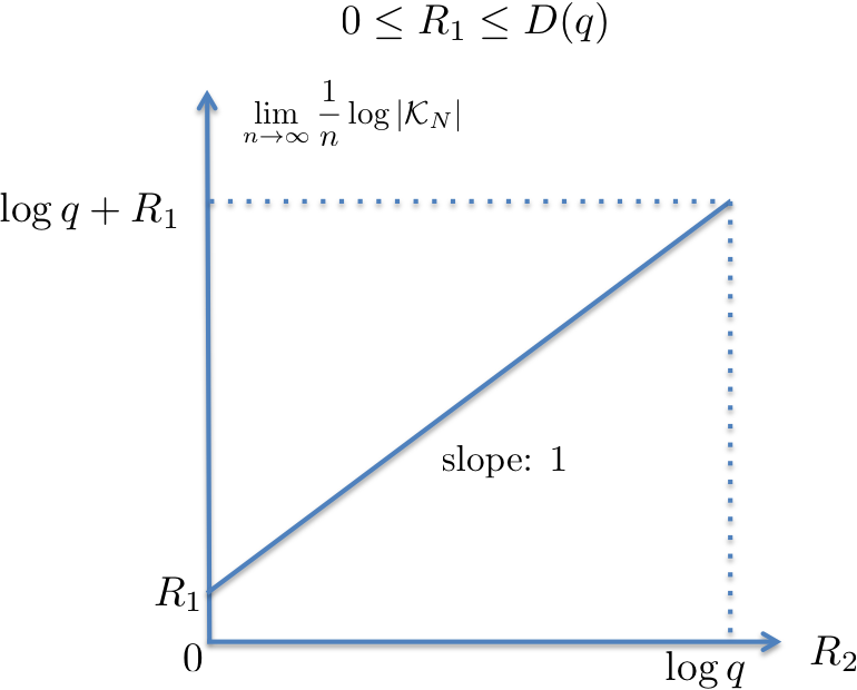
(a) For a fixed $R_{1}$ in the range $0\leq R_{1}\leq D(q)$, the normalized size of the typical sumset takes the form $\lim_{n\rightarrow\infty}\log|\mathcal{K}_{N}|/n=R_{1}+R_{2}$ as a function of $R_{2}$.

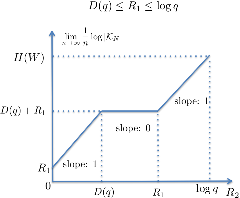
(b) For a fixed $R_{1}$ in the range $D(q)\leq R_{1}\leq\log q$, we can identify three regimes of the growth of the typical sumset. The piece-wise linear function $\lim_{n\rightarrow\infty}\frac{1}{n}\log|\mathcal{K}_{N}|$ is equal to $R_{1}+R_{2}$ for $0\leq R_{2}<D(q)$, to $D(q)+R_{1}$ for $D(q)\leq R_{2}<R_{1}$ and to $R_{2}+D(q)$ for $R_{1}\leq R_{2}\leq\log q$, as a function of $R_{2}$.

Figure 2: For a fixed $R_{1}$, the asymptotic size of the normal typical sumset $\lim_{n\rightarrow\infty}\frac{1}{n}\log|\mathcal{K}_{N}|$ as a function of $R_{2}$.

II-C The symmetric case

In the case when the two codebooks are the same, i.e., $\mathcal{C}_{1}=\mathcal{C}_{2}=\mathcal{C}$, the size of the typical sumset is easier to describe.

Corollary 1 (Normal typical sumsets–symmetric case)

Let $\mathcal{C}^{(n)}$ be a sequence linear codes indexed by their dimension in $\mathbb{F}_{q}^{n}$ with rate $R=\lim_{n\rightarrow\infty}\frac{1}{n}\log|\mathcal{C}^{(n)}|$ and let $\mathcal{C}^{\prime(n)}:=\mathcal{C}^{(n)}\oplus{\bf d}$ for any fixed ${\bf d}\in\mathbb{F}_{q}^{n}$. We assume $\mathcal{C}$ is generated as in (7) and each entry of the generator matrix ${\bf G}$ is independent and identically distributed according to the uniform distribution in $\mathbb{F}_{q}$. Then a.a.s. there exists a sequence of typical sumsets $\mathcal{K}^{(n)}_{N}\subseteq\mathcal{C}^{(n)}+\mathcal{C}^{\prime(n)}$ whose sizes satisfy

$$|\mathcal{K}_{N}^{(n)}| \doteq\begin{cases}2^{2nR}&R\leq D(q)\\ 2^{n(R+D(q))}&R>D(q)\end{cases}$$ (17)

$$D(q) :=H(U_{1}+U_{2})-\log q.$$ (18)

where $U_{1},U_{2}$ are independent variables with the distribution $P_{U}$ in (1). Furthermore for all ${\bf w}\in\mathcal{K}_{N}^{(n)}$, the induced distribution $P_{\mathcal{S}}$ defined in Definition 1 satisfies

$$P_{\mathcal{S}}({\bf w})\doteq\begin{cases}2^{-2nR}&R\leq D(q)\\ 2^{-n(R+D(q))}&R>D(q)\end{cases}$$ (19)

Proof:

This is a consequence of Theorem 1 by setting $R_{1}=R_{2}=R$. This gives

$$|\mathcal{K}_{N}^{(n)}|\doteq\min\left\{2^{2nR},2^{n(R+D(q))}\right\}.$$ (20)

It is also instructive to rewrite it in the formulation stated in the corollary. ∎

For the symmetric case, Figure 3 provides a generic plot showing the code rate $R$ vs. normalized size $\lim_{n\rightarrow\infty}\frac{1}{n}\log|\mathcal{K}_{N}^{(n)}|$ of the normal typical sumset size. We see there exists a threshold $D(q)$ on the rate $R$ of the code, above or below which the normal typical sumset $\mathcal{K}_{N}$ behaves differently. For the low rate regime $R<D(q)$, almost every codeword pair $T_{1}^{n},T_{2}^{n}$ gives a distinct sum codeword, hence the sumset size $|\mathcal{K}_{N}|$ is essentially $|\mathcal{C}|^{2}$. For the medium to high rate regime $R\geq D(q)$, due to the linear structure of the code, there are (exponentially) many different codeword pairs $T_{1}^{n},T_{2}^{n}$ which give the same sum codeword, and the normal typical sumset size $|\mathcal{K}_{N}|$ grows only as $2^{nD(q)}|\mathcal{C}|$ where $D(q)$ does not depend on $R$. In this regime the code $\mathcal{C}$ has a typical sumset which is exponentially smaller than $\mathcal{C}+\mathcal{C}^{\prime}$. In contrast to the low dimensional case where the sum of two uniformly distributed random variables is not uniformly distributed, the sum codewords are uniformly distributed in the typical sumset $\mathcal{K}_{N}$ as the dimension $n$ tends to infinity, as shown by (15) in Theorem 1. This is reminiscent of the classical typical sequences with asymptotic equipartition property (AEP), i.e., the typical sumset occurs a.a.s. but is uniformly filled up with only a small subset of sequences. We also give a pictorial description of the sum codewords $T_{1}^{n}+T_{2}^{n}$ in Figure 4.

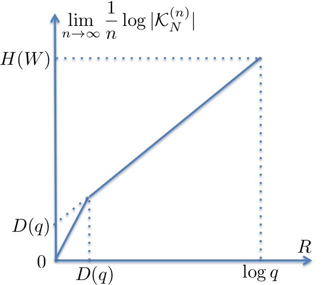
Figure 3: An illustration of the size of normal typical sumsets of linear codes in the symmetric case. $H(W)$ and $D(q)$ are given in (3) and (14), respectively. The piece-wise linear function has slope $2$ for low rate regime and slope $1$ for medium-to-high rate regime.

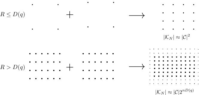
Figure 4: An illustration of the sum codewords $T_{1}^{n}+T_{2}^{n}$ in the symmetric case $\mathcal{C}_{1}=\mathcal{C}_{2}=\mathcal{C}$. For the rate $R\leq D(q)$, each pair $(T_{1}^{n},T_{2}^{n})$ will give a different sum and typical sumset $\mathcal{K}_{N}$ is essentially the same as $\mathcal{C}+\mathcal{C}$. For rate $R>D(q)$, many pairs $(T_{1}^{n},T_{2}^{n})$ give the same sum codeword and the typical sumset $\mathcal{K}_{N}$ is much smaller than $\mathcal{C}+\mathcal{C}$. Interestingly in the $n$-dimensional space with $n\rightarrow\infty$, the sum codewords $T_{1}^{n}+T_{2}^{n}$ is always uniformly distributed in the typical sumset $\mathcal{K}_{N}$ (represented by thick dots in the plot). The other sum codewords in $(\mathcal{C}+\mathcal{C})\setminus\mathcal{K}_{N}$ (represented by the small dots) have only negligible probability.

II-D Comparison with $|\mathcal{C}_{1}+\mathcal{C}_{2}|$

In Section I we emphasized the distinction between the classical sumset theory and our study of typical sumsets in a probabilistic setting. Now we compare the size of a normal typical sumset $\mathcal{K}_{N}$ of $\mathcal{C}_{1},\mathcal{C}_{2}$ with the size of the exact sumset $\mathcal{C}_{1}+\mathcal{C}_{2}$. Before doing this, we first introduce a useful result relating the sumsets of general linear codes with that of systematic linear codes.

Lemma 2 (Equivalence between systematic and non-systematic codes)

Given any linear codes $\mathcal{C}_{1},\mathcal{C}_{2}$ such that $\mathcal{C}_{2}\subseteq\mathcal{C}_{1}$, there exist systematic linear codes $\mathcal{C}_{1}^{\prime},\mathcal{C}_{2}^{\prime}$ with a one-to-one mapping $\phi:\mathcal{C}_{1}\longrightarrow\mathcal{C}_{1}^{\prime},\phi:\mathcal{C}_{2}\longrightarrow\mathcal{C}_{2}^{\prime}$ such that for any pair ${\bf t}\in\mathcal{C}_{1},{\bf v}\in\mathcal{C}_{2}$ satisfying ${\bf t}+{\bf v}={\bf s}$, we have $\phi({\bf t})+\phi({\bf v})=\phi({\bf s})$.

Proof:

A code $\mathcal{C}$ is said to be equivalent ([14, Ch. 4] ) to another code $\mathcal{C}^{\prime}$, if there exists a permutation $\pi$ over the set $\{1,\ldots,n\}$, such that every codeword ${\bf t}^{\prime}$ in $\mathcal{C}^{\prime}$ satisfies

$${\bf t}^{\prime}:=({\bf t}^{\prime}_{1},{\bf t}^{\prime}_{2},\ldots,{\bf t}^{\prime}_{n})=({\bf t}_{\pi(1)},{\bf t}_{\pi(2)},\ldots,{\bf t}_{\pi(n)})$$ (21)

for some ${\bf t}:=({\bf t}_{1},{\bf t}_{2},\ldots,{\bf t}_{n})\in\mathcal{C}$. It is known that any linear code $\mathcal{C}$ is equivalent to some systematic linear code (see [14, Ch. 4.3] for example). If we assume without loss of generality that $\mathcal{C}_{2}\subseteq\mathcal{C}_{1}$, define the mapping $\phi$ to be the permutation needed to transform the given linear code $\mathcal{C}_{1}$ to its systematic counterpart $\mathcal{C}_{1}^{\prime}$. Clearly it also gives the permutation on code $\mathcal{C}_{2}$ which transforms $\mathcal{C}_{2}$ to its systematic counterpart $\mathcal{C}_{2}^{\prime}$. Furthermore this permutation is a one-to-one mapping.

For two different pairs $({\bf t},{\bf v})$ and $(\tilde{{\bf t}},\tilde{{\bf v}})$ where ${\bf t},\tilde{{\bf t}}\in\mathcal{C}_{1},{\bf v},\tilde{{\bf v}}\in\mathcal{C}_{2}$ such that ${\bf t}+{\bf v}=\tilde{{\bf t}}+\tilde{{\bf v}}={\bf s}$, it holds that

$$\phi({\bf t})+\phi({\bf v}) =({\bf t}_{\pi(1)}+{\bf v}_{\pi(1)},{\bf t}_{\pi(2)}+{\bf v}_{\pi(2)},\ldots,{\bf t}_{\pi(n)}+{\bf v}_{\pi(n)})$$ (22)

$$=(\tilde{{\bf t}}_{\pi(1)}+\tilde{{\bf v}}_{\pi(1)},\tilde{{\bf t}}_{\pi(2)}+\tilde{{\bf v}}_{\pi(2)},\ldots,\tilde{{\bf t}}_{\pi(n)}+\tilde{{\bf v}}_{\pi(n)})$$ (23)

$$=\phi(\tilde{{\bf t}})+\phi(\tilde{{\bf v}})=\phi({\bf s})$$ (24)

where the second equality holds because of the assumption ${\bf t}+{\bf v}=\tilde{{\bf t}}+\tilde{{\bf v}}$ and the last equality holds because permutation is distributive with respect to entry-wise addition. ∎

This lemma shows that for any linear codes $\mathcal{C}_{1},\mathcal{C}_{2}$ which are nested, there exists corresponding systematic codes $\mathcal{C}_{1}^{\prime},\mathcal{C}_{2}^{\prime}$ whose sumset structure is exactly the same as the former. Now we can show the following simple bounds on the size of the sumset $\mathcal{C}_{1}+\mathcal{C}_{2}$.

Lemma 3 (Simple sumset estimates)

Let $\mathcal{C}_{1}$ be an $(n,k_{1})$-linear code and $\mathcal{C}_{2}$ an $(n,k_{2})$-linear code over $\mathbb{F}_{q}$ such that either $\mathcal{C}_{1}\subseteq\mathcal{C}_{2}$ or $\mathcal{C}_{2}\subseteq\mathcal{C}_{1}$. The size of the sumset $\mathcal{C}_{1}+\mathcal{C}_{2}$ is upper bounded as

$$|\mathcal{C}_{1}+\mathcal{C}_{2}|\leq q^{k_{1}+k_{2}}$$ (25)

and lower bounded as

$$|\mathcal{C}_{1}+\mathcal{C}_{2}|\geq(2q-2)^{\min(k_{1},k_{2})}$$ (26)

Proof:

The upper bound follows simply from the fact that $|\mathcal{C}_{1}+\mathcal{C}_{2}|\leq|\mathcal{C}_{1}||\mathcal{C}_{2}|$ for any set $\mathcal{C}_{1},\mathcal{C}_{2}$. To establish the lower bound, Lemma 2 shows that for any nested linear code $\mathcal{C}_{1},\mathcal{C}_{2}$, we can find corresponding systematic linear codes $\mathcal{C}_{1}^{\prime},\mathcal{C}_{2}^{\prime}$ whose sumset size $|\mathcal{C}_{1}^{\prime}+\mathcal{C}_{2}^{\prime}|$ equals to $|\mathcal{C}_{1}+\mathcal{C}_{2}|$. The lower bound follows by noticing that for any systematic linear codes, the sum of the message part of the codewords already take at least $(2q-2)^{\min(k_{1},k_{2})}$ different values. ∎

Notice $|\mathcal{K}_{N}|$ can be smaller than the simple lower bound given in (26) for certain rate range. The reason is clear: some of the sum codewords $T_{1}^{n}+T_{2}^{n}$ occurs very rarely if $T_{1}^{n}$ and $T_{2}^{n}$ are chosen uniformly. Those sum codewords will be counted in the sumset $\mathcal{C}_{1}+\mathcal{C}_{2}$ but are probabilistically negligible. For a comparison, we consider the simple case when $k_{1}=k_{2}$ hence $\mathcal{C}_{1}$ and $\mathcal{C}_{2}$ are identical. we see the lower bound in (26) states that

$$|\mathcal{C}_{1}+\mathcal{C}_{2}|\geq 2^{nR_{1}\log(2q-2)/\log q}.$$ (27)

Then Eq. (13) implies that $|\mathcal{K}_{N}|$ is smaller than $|\mathcal{C}_{1}+\mathcal{C}_{2}|$ for the rate range

$$R>\frac{D(q)}{\log(2q-2)/\log q-1},$$ (28)

(Notice that the RHS is always larger than $D(q)$ for $q\geq 2$ but is only meaningful if it is smaller than $\log q$). For example $|\mathcal{K}_{N}|$ is smaller than the lower bound in (26) for $R>2.85$ bits with $q=11$ and for $R>4.87$ bits for $q=101$.

II-E Entropy of sumsets

Often we are interested in inequalities relating the entropy of two random variables $X_{1},X_{2}$ and the entropy of their sum $X_{1}+X_{2}$. One classical result is the entropy power inequality involving differential entropy. Recent works including [11] [12] have established several fundamental results on this topic. For our problem, if codes $\mathcal{C}_{1},\mathcal{C}_{2}$ have a normal typical sumset and $T_{1}^{n},T_{2}^{n}$ are random variables uniformly distributed in $\mathcal{C}_{1},\mathcal{C}_{2}$ respectively, we are able to give an asymptotic relationship between $H(T_{1}^{n}),H(T_{2}^{n})$ and $H(T_{1}^{n}+T_{2}^{n})$.

Theorem 2 (Entropy of sumsets)

Let $\mathcal{C}_{1}^{(n)},\mathcal{C}_{2}^{(n)}$ be two sequences of linear codes in $\mathbb{F}_{q}^{n}$ with normal typical sumsets $\mathcal{K}_{N}^{(n)}$ as in Theorem 1. Let $T_{1}^{n},T_{2}^{n}$ be independent random $n$-length vectors uniformly distributed in the code $\mathcal{C}_{1}^{(n)},\mathcal{C}_{2}^{(n)}$, respectively. In the limit $n\rightarrow\infty$ we have

$$\lim_{n\rightarrow\infty}\frac{H(T_{1}^{n}+T_{2}^{n})}{n} =\min\left\{\frac{H(T^{n}_{1})+H(T^{n}_{2})}{n},\frac{\max\{H(T^{n}_{1}),H(T^{n}_{2})\}}{n}+D(q)\right\}$$ (29)

$$=\min\{R_{1}+R_{2},\max\{R_{1},R_{2}\}+D(q)\}$$ (30)

where as before, $D(q):=H(W)-\log q$ with $W$ distributed according to $P_{W}$ in (2).

Proof:

As $T_{j}^{n},j=1,2$ is uniformly distributed in the $(n,k_{j})$-linear code $\mathcal{C}_{j}$ with rate $R_{j}$, we have $H(T_{j}^{n})=nR_{j}$. Theorem 1 shows that the distribution of the random variable $T_{1}^{n}+T_{2}^{n}$ depends on the values $R_{1}+R_{2}$ and $\max\{R_{1},R_{2}\}+D(q)$. We first consider the case when the $R_{1}+R_{2}$ is smaller than the latter value. Recall that $P_{\mathcal{S}}$ denotes the distribution on $\mathcal{C}_{1}+\mathcal{C}_{2}$ induced by $T_{1}^{n},T_{2}^{n}$ as in Definition 1, we have

$$H(T_{1}^{n}+T_{2}^{n}) =-\sum_{{\bf w}\in\mathcal{C}_{1}+\mathcal{C}_{2}}P_{\mathcal{S}}({\bf w})\log P_{\mathcal{S}}({\bf w})$$ (31)

$$\geq-\sum_{{\bf w}\in\mathcal{K}_{N}}P_{\mathcal{S}}({\bf w})\log P_{\mathcal{S}}({\bf w})$$ (32)

Theorem 1 shows that in this case for ${\bf w}\in\mathcal{K}_{N}$ it holds that $P_{\mathcal{S}}({\bf w})\leq 2^{-n(R_{1}+R_{2}-\epsilon_{n})}$, hence

$$H(T_{1}^{n}+T_{2}^{n}) \geq-\log 2^{-n(R_{1}+R_{2}-\epsilon_{n})}\sum_{{\bf w}\in\mathcal{K}_{N}}P_{\mathcal{S}}({\bf w})$$ (33)

$$=n(R_{1}+R_{2}-\epsilon_{n})(1-\delta_{n})$$ (34)

with $\delta_{n}\rightarrow 0$ because $\mathcal{K}_{N}$ is a typical sumset. It follows that

$$\lim_{n\rightarrow\infty}H(T_{1}^{n}+T_{2}^{n})/n \geq\lim_{n\rightarrow\infty}(R_{1}+R_{2}-\epsilon_{n})(1-\delta_{n})$$ (35)

$$=R_{1}+R_{2}=(H(T_{1})+H(T_{2}))/n$$ (36)

as both $\delta_{n},\epsilon_{n}\rightarrow 0$.

On the other hand, we have

$$H(T_{1}^{n}+T_{2}^{n}) =-\sum_{{\bf w}\in\mathcal{K}_{N}}P_{\mathcal{S}}({\bf w})\log P_{\mathcal{S}}({\bf w})-\sum_{{\bf w}\notin\mathcal{K}_{N}}P_{\mathcal{S}}({\bf w})\log P_{\mathcal{S}}({\bf w})$$ (37)

For ${\bf w}\in\mathcal{K}_{N}$ it holds $P_{\mathcal{S}}({\bf w})\geq 2^{-n(R_{1}+R_{2}+\epsilon_{n})}$ in this case, implied by Theorem 1. Hence the first term above is bounded as

$$-\sum_{{\bf w}\in\mathcal{K}_{N}}P_{\mathcal{S}}({\bf w})\log P_{\mathcal{S}}({\bf w}) \leq-\log 2^{-n(R_{1}+R_{2}+\epsilon_{n})}\sum_{{\bf w}\in\mathcal{K}_{N}}P_{\mathcal{S}}({\bf w})$$ (38)

$$\leq n(R_{1}+R_{2}+\epsilon_{n})$$ (39)

To bound the second term, using log sum inequatliy [13, Lemma 3.1] gives

$$-\sum_{{\bf w}\notin\mathcal{K}_{N}}P_{\mathcal{S}}({\bf w})\log P_{\mathcal{S}}({\bf w}) \leq-\left(\sum_{{\bf w}\notin\mathcal{K}_{N}}P_{\mathcal{S}}({\bf w})\right)\log\frac{\sum_{{\bf w}\notin\mathcal{K}_{N}}P_{\mathcal{S}}({\bf w})}{|\overline{\mathcal{K}_{N}}|}$$ (40)

$$=-P_{\mathcal{S}}(\overline{\mathcal{K}_{N}})\log P_{\mathcal{S}}(\overline{\mathcal{K}_{N}})+P_{\mathcal{S}}(\overline{\mathcal{K}_{N}})\log|\overline{\mathcal{K}_{N}}|$$ (41)

where $\overline{\mathcal{K}_{N}}$ denotes the complementary set $(\mathcal{C}_{1}+\mathcal{C}_{2})\backslash\mathcal{K}_{N}$. Later in Lemma 4 Eq. (57) we show that

$$P_{\mathcal{S}}(\overline{\mathcal{K}_{N}})\leq 4qe^{-n\delta^{2}\min\{R_{1},R_{2}\}/\log q}$$ (42)

For $n\rightarrow\infty$, the first term in (41) approaches zero as $P_{\mathcal{S}}(\overline{\mathcal{K}_{N}})\rightarrow 0$. The second term is bounded as

$$P_{\mathcal{S}}(\overline{\mathcal{K}_{N}})\log|\overline{\mathcal{K}_{N}}| \leq 4qe^{-n\delta^{2}\min\{R_{1},R_{2}\}/\log q}\log 2^{n(R_{1}+R_{2})}$$ (43)

$$=4n(R_{1}+R_{2})qe^{-n\delta^{2}\min\{R_{1},R_{2}\}/\log q}$$ (44)

approaches zero as well for large enough $n$. Hence overall we have

$$\lim_{n\rightarrow\infty}H(T_{1}^{n}+T_{2}^{n}) \leq\lim_{n\rightarrow\infty}(R_{1}+R_{2}+\epsilon_{n})+o_{n}(1)$$ (45)

$$=n(R_{1}+R_{2})=(H(T_{1}^{n})+H(T_{2}^{n}))/n$$ (46)

This shows in the limit we have $H(T_{1}^{n}+T_{2}^{n})/n\rightarrow(H(T_{1}^{n})+H(T_{2}^{n}))/n$ for the case $R_{1}+R_{2}\leq\max\{R_{1},R_{2}\}+D(q)$. The other case can be proved in the same way.∎

III Proof of Theorem 1

We prove Theorem 1 in a few steps. Lemma 2 already shows that for any linear codes $\mathcal{C}_{1},\mathcal{C}_{2}$, there exist corresponding systematic linear codes whose sumset structure is the same as the former. Hence we first focus on systematic linear codes and establish a similar result. Given two matrices ${\bf Q}\in\mathbb{F}_{q}^{(n-k_{1})\times k_{1}}$ and ${\bf H}\in\mathbb{F}_{q}^{(k_{1}-k_{2})\times k_{2}}$ with $k_{1}\geq k_{2}$, we consider two codes of the form

$$\mathcal{C}_{1} =\left\{{\bf t}:{\bf t}=\begin{bmatrix}{\bf I}_{k_{1}\times k_{1}}\\ {\bf Q}\end{bmatrix}{\bf m},\mbox{ for all }{\bf m}\in\mathbb{F}_{q}^{k_{1}}\right\}$$ (47a)

$$\mathcal{C}_{2} =\left\{{\bf v}:{\bf v}=\begin{bmatrix}{\bf I}_{k_{1}\times k_{1}}\\ {\bf Q}\end{bmatrix}{\bf n}=\begin{bmatrix}{\bf I}_{k_{1}\times k_{1}}\\ {\bf Q}\end{bmatrix}\begin{bmatrix}{\bf n}^{\prime}\\ {\bf H}{\bf n}^{\prime}\end{bmatrix},\mbox{ for all }{\bf n}^{\prime}\in\mathbb{F}_{q}^{k_{2}}\right\}$$ (47b)

where we defined ${\bf n}:=\begin{bmatrix}{\bf n}^{\prime}\\ {\bf H}{\bf n}^{\prime}\end{bmatrix}$. It is easy to see that we have $\mathcal{C}_{2}\subseteq\mathcal{C}_{1}$ in this case. Also notice that it is in general insufficient to set ${\bf H}$ to be the zero matrix. For example for the case $k_{1}=n$, letting ${\bf H}$ to be the zero matrix will result in a $\mathcal{C}_{2}$ whose codewords do not have parity part.

Theorem 3 (Normal typical sumset - systematic linear codes)

Let $\mathcal{C}_{1}^{(n)},\mathcal{C}_{2}^{(n)}$ be two sequences of systematic linear codes in the form (47) indexed by their dimension. The rates of the two codes are given by $R_{j}=\lim_{n\rightarrow\infty}\frac{1}{n}\log|\mathcal{C}_{j}^{(n)}|$ for $j=1,2$. For any fixed vector ${\bf d}\in\mathbb{F}_{q}^{n}$ define $\mathcal{C}_{1}^{\prime(n)}:=\mathcal{C}_{1}^{(n)}\oplus{\bf d}$ as in (12). If each entry of the matrices ${\bf Q},{\bf H}$ is independent and identically distributed according to the uniform distribution in $\mathbb{F}_{q}$, then asymptotically almost surely there exists a sequence of typical sumsets $\mathcal{K}_{N}^{(n)}\subseteq\mathcal{C}_{1}^{\prime(n)}+\mathcal{C}_{2}^{(n)}$ with sizes given in (13). Furthermore, the induced probability distribution $P_{\mathcal{S}}$ on $\mathcal{C}_{1}^{\prime(n)}+\mathcal{C}_{2}^{(n)}$ satisfies (15).

Remark 2

There exist linear codes with a smaller typical sumset than $|\mathcal{K}_{N}|$. As an extreme example consider the sumset $\mathcal{C}+\mathcal{C}$ where a systematic $(n,k)$-linear codes $\mathcal{C}$ is generated with the generator matrix $[{\bf I};{\bf 0}]$, i.e., the ${\bf Q}$ matrix is the zero matrix. Since the sum codewords are essentially $k$-length sequences with each entry i.i.d. with distribution $P_{W}$, it is easy to see that the set of typical sequences $\mathcal{A}_{[W]}^{k}$ is actually a typical sumset for this code with size $2^{kH(W)}=2^{nRH(W)/\log q}$ where $W$ has the distribution in (2). This code has a typical sumset which is smaller than the normal typical sumset as demonstrated in Figure 5. However this kind of codes are rare and the above theorem states that a randomly picked systematic linear code has a normal typical sumset a.a.s..

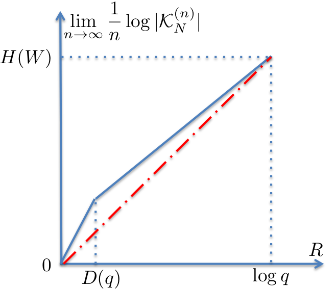
Figure 5: A linear code with a typical sumset which is not normal: the solid line shows the size of the normal typical sumset and the dot-dashed line shows the size of a typical sumset of the example in Remark 2. This code has a small typical sumset with size $2^{nRH(W)/\log q}$ but is uninteresting for the purpose of error corrections.

We first prove Theorem 3. In the following we will always assume without loss of generality that $k_{1}\geq k_{2}$. Let $\mathcal{C}_{1}$ be an $(n,k_{1})$-systematic linear code and $\mathcal{C}_{2}$ be an $(n,k_{2})$-systematic linear code generated using the same generator matrix $[{\bf I};{\bf Q}]$ as in (47). We fix a vector ${\bf d}$ and let $\mathcal{C}_{1}^{\prime}=\mathcal{C}_{1}\oplus{\bf d}$ as in (12). We use ${\bf d}_{1}$ to denote the first $k_{1}$ entries of ${\bf d}$, ${\bf d}_{2}$ to denote the entries from $k_{1}-k_{2}$ to $k_{1}$ and ${\bf d}_{3}$ the last $n-k_{1}$ entries of ${\bf d}$. Assume two messages ${\bf m},{\bf n}^{\prime}$ are independently and uniformly chosen from $\mathbb{F}_{q}^{k_{1}},\mathbb{F}_{q}^{k_{2}}$, respectively, and two codewords ${\bf t}\in\mathcal{C}_{1}$, ${\bf v}\in\mathcal{C}_{2}$ are formed using ${\bf m},{\bf n}^{\prime}$ as in (47). The sum codeword of $\mathcal{C}_{1}^{\prime}+\mathcal{C}_{2}$ can be written as

$$({\bf t}\oplus{\bf d})+{\bf v}=\begin{bmatrix}({\bf m}_{1}\oplus{\bf d}_{1})+{\bf n}^{\prime}\\ ({\bf m}_{2}\oplus{\bf d}_{2})+{\bf H}{\bf n}^{\prime}\\ ({\bf Q}{\bf m}\oplus{\bf d}_{3})+{\bf Q}{\bf n}\end{bmatrix}:=\begin{bmatrix}\sf s({\bf m},{\bf n}^{\prime})\\ \sf p_{1}({\bf m},{\bf n}^{\prime})\\ \sf p_{2}({\bf m},{\bf n}^{\prime})\end{bmatrix}$$ (48)

where we use ${\bf m}_{1}$ to denote the first $k_{2}$ entries of ${\bf m}$ and ${\bf m}_{2}$ to denote its remaining entries. We use $\sf s({\bf m},{\bf n}^{\prime})$ to denote the first $k_{2}$ entries of the sum codewords. We also use $\sf p_{1}({\bf m},{\bf n}^{\prime})$ and $\sf p_{2}({\bf m},{\bf n}^{\prime})$ to denote the entries of the sum codewords with indices ranging from $k_{2}$ to $k_{1}$, and with indices ranging from $k_{1}$ to $n$, respectively. In the sequel we will refer to $\sf s({\bf m},{\bf n}^{\prime})$ and $\sf p_{1}({\bf m},{\bf n}^{\prime}),\sf p_{2}({\bf m},{\bf n}^{\prime})$ defined above as the information-sum and parity-sum, respectively. We shall omit their dependence on ${\bf m},{\bf n}^{\prime}$ and use $\sf s,\sf p_{1},\sf p_{2}$ if it is clear in the context.

We choose $\mathcal{K}_{N}$ to be the set which contains sum codewords whose information-sum ${\bf s}$ is typical, that is

$$\mathcal{K}_{N}:=\left\{({\bf t}\oplus{\bf d})+{\bf v}\middle|({\bf t}\oplus{\bf d})+{\bf v}=\begin{bmatrix}\sf s\\ {\sf p}_{1}\\ {\sf p}_{2}\end{bmatrix}\text{ where }{\sf s}\in\mathcal{A}^{(k_{2})}_{[W]}\right\}$$ (49)

with ${\sf s},{\sf p}_{1},{\sf p}_{2}$ defined in (48) and $W$ defined in (2). For all pairs of codewords $({\bf t},{\bf v})$ whose information-sum equals to a common value ${\bf s}$, we define the set of all possible parity-sums as

$$\mathcal{P}_{{\bf Q},{\bf H}}({\bf s}):=\left\{\begin{bmatrix}({\bf m}_{2}\oplus{\bf d}_{2})+{\bf H}{\bf n}^{\prime}\\ ({\bf Q}{\bf m}\oplus{\bf d}_{3})+{\bf Q}{\bf n}\end{bmatrix}:{\bf m}\in\mathbb{F}_{q}^{k_{1}},{\bf n}^{\prime}\in\mathbb{F}_{q}^{k_{2}}\mbox{ such that }\sf s({\bf m},{\bf n}^{\prime})={\bf s}\right\}.$$ (50)

with ${\bf n}:=\begin{bmatrix}{\bf n}^{\prime}\\ {\bf H}{\bf n}^{\prime}\end{bmatrix}$. To facilitate our analysis, we further decompose the above set in the following way. When the information-sum is fixed to be $\sf s({\bf m},{\bf n}^{\prime})={\bf s}$, we define the set of possible parity-sums $\sf p_{1}$ as

$$\mathcal{P}_{1,{\bf H}}({\bf s}):=\left\{({\bf m}_{2}\oplus{\bf d}_{2})+{\bf H}{\bf n}^{\prime}:{\bf m}\in\mathbb{F}_{q}^{k_{1}},{\bf n}^{\prime}\in\mathbb{F}_{q}^{k_{2}}\mbox{ such that }\sf s({\bf m},{\bf n}^{\prime})={\bf s}\right\}.$$ (51)

When the information-sum $\sf s$ is fixed to be $\sf s({\bf m},{\bf n}^{\prime})={\bf s}$ and the parity-sum $\sf p_{1}$ is fixed to be ${\sf p}_{1}({\bf m},{\bf n}^{\prime})={\bf p}_{1}$, we also define the set of possible parity-sums ${\sf p}_{2}$ as

$$\mathcal{P}_{2,{\bf Q},{\bf H}}({\bf s},{\bf p}_{1}):=\left\{({\bf Q}{\bf m}\oplus{\bf d}_{3})+{\bf Q}{\bf n}:{\bf m}\in\mathbb{F}_{q}^{k_{1}},{\bf n}^{\prime}\in\mathbb{F}_{q}^{k_{2}}\mbox{ such that }{\sf s}({\bf m},{\bf n}^{\prime})={\bf s},{\sf p}_{1}({\bf m},{\bf n}^{\prime})={\bf p}_{1}\right\}.$$ (52)

Notice we have the following relationship between the cardinality of the above three sets

$$|\mathcal{P}_{{\bf Q},{\bf H}}({\bf s})|=\sum_{{\bf p}_{1}\in\mathcal{P}_{1,{\bf H}}({\bf s})}|\mathcal{P}_{2,{\bf Q},{\bf H}}({\bf s},{\bf p}_{1})|$$ (53)

In the following lemma we show that the set $|\mathcal{K}_{N}|$ defined in (49) is indeed a typical sumset. We also give a simple estimate on its size.

Lemma 4 (The typical sumset $|\mathcal{K}_{N}|$)

Let $\mathcal{C}_{1}$ be an $(n,k_{1})$-systematic linear code and $\mathcal{C}_{2}$ an $(n,k_{2})$-systematic linear code ($k_{1}\geq k_{2}$) which are generated as in (47). Let $\mathcal{C}_{1}^{\prime}=\mathcal{C}_{1}\oplus{\bf d}$ for any fixed ${\bf d}$ and $T_{1}^{n},T_{2}^{n}$ be two random variables uniformly distributed in $\mathcal{C}_{1}^{\prime},\mathcal{C}_{2}$, respectively. We have

$$\mathbb{P}\left\{T_{1}^{n}+T_{2}^{n}\in\mathcal{K}_{N}\right\}\rightarrow 1\mbox{ as }n\rightarrow\infty$$ (54)

with $\mathcal{K}_{N}$ defined in (49). Furthermore we have

$$|\mathcal{K}_{N}|=\sum_{{\bf s}\in\mathcal{A}^{(k_{2})}_{[W]}}|\mathcal{P}_{{\bf Q},{\bf H}}({\bf s})|$$

with $W$ defined in (2).

Proof:

Recall that we defined $\mathcal{K}_{N}$ in (49) to be the set containing all sum codewords whose information-sum $\sf s$ satisfies the property that $\sf s$ is a typical sequence in $\mathcal{A}^{(k_{2})}_{[W]}$. As shown in (48) $\sf s={\bf m}_{1}\oplus{\bf d}_{1}+{\bf n}^{\prime}$ where ${\bf m}_{1}$ and ${\bf u}^{\prime}$ are independent vectors and are uniformly distributed in $\mathcal{U}^{k_{2}}$, then for any fixed ${\bf d}$, the first $k_{2}$ entries of $T_{1}^{n}+T_{2}^{n}$ is in fact an i.i.d. sequence distributed according to $P_{W}$, thanks to the systematic form of the codes.

Let $S^{k_{2}}$ denote a $k_{2}$-length random vector with each entry i.i.d. according to $P_{W}$. We have

$$\mathbb{P}\left\{T_{1}^{n}+T_{2}^{n}\in\mathcal{K}_{N}\right\} =\mathbb{P}\left\{S^{k_{2}}\in\mathcal{A}^{(k_{2})}_{[W]}\right\}$$ (55)

$$\geq(1-2|\mathcal{W}|e^{-2k_{2}\delta^{2}})$$ (56)

$$>1-4qe^{-n(2\delta^{2}R_{2}/\log q)}$$ (57)

where the first inequality follows from the property of typical sequences in Lemma 1. Choose $\delta$ such that $n\delta^{2}\rightarrow\infty$, we have that $T_{1}^{n}+T_{2}^{n}\in\mathcal{K}_{N}$ a.a.s. for $n$ large enough and $R_{2}>0$. This shows $\mathcal{K}_{N}$ is indeed a typical sumset. The claim on the size of $\mathcal{K}_{N}$ follows by the definition of $\mathcal{K}_{N}$ and $\mathcal{P}_{{\bf Q},{\bf H}}({\bf s})$. ∎

The above lemma shows that we only need to focus on the message pairs $({\bf m},{\bf n}^{\prime})$ if the information-sum ${\sf s}({\bf m},{\bf n}^{\prime})$ is a typical sequence ${\bf s}\in\mathcal{A}_{[W]}^{(k_{2})}$ as shown in (49). For a given information-sum ${\bf s}$, we have the following characterization.

Lemma 5 (Message pairs with given $\sf s$)

Let ${\bf m},{\bf n}^{\prime}$ be two vectors in $\mathbb{F}_{q}^{k_{1}}$ and $\mathbb{F}_{q}^{k_{2}}$ respectively. Two codes $\mathcal{C}_{1},\mathcal{C}_{2}$ with rate $R_{1},R_{2}$ are generated as in (47) and their sum codewords are of the form in (48). There are $L$ pairs of $({\bf m},{\bf n}^{\prime})$ satisfying $\sf s({\bf m},{\bf n}^{\prime})={\bf s}$ for some ${\bf s}\in\mathcal{A}_{[W]}^{(k_{2})}$ with

$$L\doteq 2^{n(R_{1}+R_{2}-R_{2}H(W)/\log q)}$$

Proof:

Recall that for any fixed ${\bf d}$, we defined ${\sf s}({\bf m},{\bf n}^{\prime}):=({\bf m}_{1}\oplus{\bf d}_{1})+{\bf n}^{\prime}$ where ${\bf m}_{1},{\bf d}_{1}$ is given in (48). For a given value ${\bf s}_{i}\in\mathcal{W}$, we can write out all possible $({\bf m}_{1,i}\oplus{\bf d}_{1,i},{\bf n}_{i})$ summing up to ${\bf s}_{i}$ explicitly:

$${\bf s}_{i}: ({\bf m}_{1,i}\oplus{\bf d}_{1,i},{\bf n}^{\prime}_{i})\mbox{ such that }{\bf m}_{1,i}\oplus{\bf d}_{1,i}+{\bf n}^{\prime}_{i}={\bf s}_{i},i=1,\ldots,k_{2}$$

$$0: (0,0)$$

$$1: (0,1),(1,0)$$

$$2: (1,1),(2,0),(0,2)$$

$$3: (0,3),(3,0),(1,2),(2,1)$$

$$\vdots$$

$$q-1: (0,q-1),(q-1,0),(1,q-2),(q-2,1),\ldots,((q-1)/2,(q-1)/2)$$

$$\vdots$$

$$2q-3: (q-1,q-2),(q-2,q-1)$$

$$2q-2: (q-1,q-1)$$

We can show that the number of different pairs $({\bf m}_{1}\oplus{\bf d}_{1},{\bf n}^{\prime})$ satisfying ${\bf m}_{1}\oplus{\bf d}_{1}+{\bf n}^{\prime}={\bf s}$ is

$$2^{(2/q^{2}+o(1))k_{2}}3^{(3/q^{2}+o(1))k_{2}}\ldots q^{(q/q^{2}+o(1))k_{2}}(q-1)^{((q-1)/q^{2}+o(1))k_{2}}\ldots 2^{(2/q^{2}+o(1))k_{2}}$$ (58)

$$=\prod_{a=1}^{q}a^{(a/q^{2}+o(1))k_{2}}\prod_{a=1}^{q-1}a^{(a/q^{2}+o(1))k_{2}}$$ (59)

$$=2^{k_{2}(\log q-D(q)+o(1))}$$ (60)

To see why this is the case, recall that since ${\bf s}$ is a typical sequence in $\mathcal{A}_{[W]}^{(k_{2})}$, there are for example $(2/q^{2}+o(1))k_{2}$ entries in ${\bf s}$ taking value $1$, as implied by the definition of typical sequences in (4) and the distribution $P_{W}$. The pair $({\bf m}_{1,i}\oplus{\bf d}_{1,i},{\bf n}^{\prime}_{i})$ can take value $(1,0)$ or $(0,1)$ in these entries. Hence there are $2^{(2/q^{2}+o(1))k_{2}}$ different choices on the pair $({\bf m}_{1}\oplus{\bf d}_{1},{\bf n}^{\prime})$ for those entries. The same argument goes for other entries taking values $2,\ldots,2q-2$ using the number of possible values of $({\bf m}_{1,i}\oplus{\bf d}_{1,i},{\bf n}^{\prime}_{i})$ shown in the above list. Furthermore since there are $q^{k_{1}-k_{2}}$ possible ${\bf m}_{2}$ for each of the $({\bf m}_{1}\oplus{\bf d}_{1},{\bf n}^{\prime})$, the number of $({\bf m},{\bf n}^{\prime})$ giving ${\sf s}({\bf m},{\bf n}^{\prime})={\bf s}$ is

$$L=2^{k_{2}(\log q-D(q)+o(1))}\cdot q^{k_{1}-k_{2}}\doteq 2^{n(R_{1}+R_{2}-R_{2}H(W)/\log q)}$$

which proves the claim. ∎

In the following lemmas we will give the estimates on the size of parity-sums.

Lemma 6 (Estimates of $|\mathcal{P}_{1}|$)

Let ${\bf m},{\bf n}^{\prime}$ be two independent random vectors which are uniformly distributed in $\mathbb{F}_{q}^{k_{1}}$ and $\mathbb{F}_{q}^{k_{2}}$, respectively. For the pairs $({\bf m},{\bf n}^{\prime})$ satisfying ${\sf s}({\bf m},{\bf n}^{\prime})={\bf s}$ for some ${\bf s}\in\mathcal{A}_{[W]}^{(k_{2})}$, let $\mathcal{P}_{1}({\bf s})$ denote the random set formed in (51), where each entry of ${\bf H}$ is i.i.d. according to the uniform distribution in $\mathbb{F}_{q}$. Then asymptotically almost surely it holds that

$$|\mathcal{P}_{1}({\bf s})|\doteq 2^{n(R_{1}+R_{2}-R_{2}H(W)/\log q)}$$

if $R_{2}\leq R_{1}D(q)/\log q$, and

$$|\mathcal{P}_{1}({\bf s})|\doteq 2^{n(R_{1}-R_{2})H(W)/\log q}$$

if $R_{2}\geq R_{1}D(q)/\log q$.

Proof:

We will bound the possible number of different parity-sum ${\sf p}_{1}$ given the condition that ${\sf s}({\bf m},{\bf n}^{\prime})={\bf s}$ for some ${\bf s}\in\mathcal{A}_{[W]}^{(k_{2})}$. It is shown in Appendix D, Lemma 10 that each entry of the parity sum ${\sf p}_{1}$ is i.i.d. according to $P_{W}$ hence the probability that the parity-sum ${\sf p}_{1}$ being atypical is negligible. For a given typical vector ${\bf p}\in\mathcal{A}^{(k_{1}-k_{2})}_{[W]}$, define the random variable $Z_{1}({\bf p})$ to be the number of pairs $({\bf m},{\bf n}^{\prime})$ whose parity sum $\sf p_{1}$ is equal to ${\bf p}$. In other words, define the random set

$$\mathcal{Z}_{1}({\bf p}):=\{({\bf m},{\bf n}^{\prime}):{\bf m}_{2}\oplus{\bf d}_{2}+{\bf H}{\bf n}^{\prime}={\bf p}\}$$

where each entry of ${\bf H}$ is chosen uniformly at random from $\mathbb{F}_{q}$, the random variable $Z_{1}({\bf p})$ is defined as $Z_{1}({\bf p}):=|\mathcal{Z}_{1}({\bf p})|$. In Appendix B we show that if $\sf s({\bf m},{\bf n}^{\prime})={\bf s}$ for some ${\bf s}\in\mathcal{A}_{[W]}^{(k_{2})}$ and with randomly chosen ${\bf H}$, the conditional expectation and variance of $Z_{1}({\bf p})$ for a typical sequence ${\bf p}\in\mathcal{A}^{(k_{1}-k_{2})}_{[W]}$ is bounded as

$$2^{n\left(R_{2}-R_{1}D(q)/\log q-\epsilon_{n}\right)}\leq{\rm I\kern-3.00003ptE}\left[Z_{1}({\bf p})|\sf s({\bf m},{\bf n}^{\prime})={\bf s}\right]\leq 2^{n\left(R_{2}-R_{1}D(q)/\log q+\epsilon_{n}\right)}$$ (61)

for some $\epsilon_{n}\rightarrow 0$. For any fixed ${\bf p}\in\mathcal{A}^{(k_{1}-k_{2})}_{[W]}$, Markov inequality shows that

$$\mathbb{P}\left\{Z_{1}({\bf p})>1)|\sf s({\bf m},{\bf n}^{\prime})={\bf s}\right\} \leq{\rm I\kern-3.00003ptE}\left[Z_{1}({\bf p})|\sf s({\bf m},{\bf n}^{\prime})={\bf s}\right]\leq 2^{n\left(R_{2}-R_{1}D(q)/\log q+\epsilon_{n}\right)}$$ (62)

In the case when $R_{2}\leq R_{1}D(q)/\log q-2\epsilon_{n}$, we have $\mathbb{P}\left\{Z_{1}({\bf p})>1|{\sf s}({\bf m},{\bf n}^{\prime})={\bf s}\right\}\leq 2^{-n\epsilon_{n}}$ which can be made arbitrarily small for large enough $n$ if choose $\epsilon_{n}$ such that $n\epsilon_{n}\rightarrow\infty$. As $Z_{1}({\bf p})$ denotes the number of pairs $({\bf m},{\bf n}^{\prime})$ which give a parity-sum as $\sf p_{1}({\bf m},{\bf n}^{\prime})={\bf p}$, this means a.a.s. any typical sequence ${\bf p}$ can be formed by at most one pair $({\bf m},{\bf n}^{\prime})$. In other words, every pair will form a distinct $\sf p_{1}({\bf m},{\bf n}^{\prime})$ a.a.s. hence the number of distinct ${\sf p}_{1}$ equals to the number of pairs $({\bf m},{\bf n}^{\prime})$ satisfying ${\sf s}({\bf m},{\bf n}^{\prime})={\bf s}$, which is given by $L$ in Lemma 5. This proves the first claim by letting $\epsilon_{n}$ go to zero.

In the case when $R_{2}\geq R_{1}D(q)/\log q$, we show that the number of different $\sf p_{1}$ is concentrated around $2^{n(R_{1}-R_{2})H(W)/\log q}$. For some $\epsilon^{\prime}_{n}>0$ depending on $n$, by conditional Chebyshev inequality (see [15, Ch. 23.4] for example) we have

$$\mathbb{P}\left\{|Z_{1}({\bf p})-{\rm I\kern-3.00003ptE}\left[Z_{1}({\bf p})\right]|\geq 2^{\frac{n}{2}\left(R_{2}-R_{1}D(q)/\log q+\epsilon^{\prime}_{n}\right)}|{\sf s}({\bf m},{\bf n}^{\prime})={\bf s}\right\} \leq\frac{\mbox{Var}\left[Z_{1}({\bf p})|{\sf s}({\bf m},{\bf n}^{\prime})={\bf s}\right]}{2^{2\cdot\frac{n}{2}\left(R_{2}-R_{1}D(q)/\log q+\epsilon^{\prime}_{n}\right)}}$$ (63)

$$\leq\frac{{\rm I\kern-3.00003ptE}\left[Z_{1}({\bf p})|{\sf s}({\bf m},{\bf n}^{\prime})={\bf s}\right]}{2^{2\cdot\frac{n}{2}\left(R_{2}-R_{1}D(q)/\log q+\epsilon^{\prime}_{n}\right)}}$$ (64)

$$\leq 2^{-n(\epsilon^{\prime}_{n}-\epsilon_{n})}$$ (65)

where we used the inequality $\mbox{Var}\left[Z_{1}({\bf p})|{\sf s}({\bf m},{\bf n}^{\prime})={\bf s}\right]\leq{\rm I\kern-3.00003ptE}\left[Z_{1}({\bf p})|{\sf s}({\bf m},{\bf n}^{\prime})={\bf s}\right]$ proved in Appendix B. If we choose $\epsilon^{\prime}_{n}>\epsilon_{n}$ and $n$ such that $n(\epsilon^{\prime}_{n}-\epsilon_{n})\rightarrow\infty$ and $\epsilon^{\prime}_{n}\rightarrow 0$ (this is possible because $\epsilon_{n}\rightarrow 0$), then under the condition that ${\sf s}({\bf m},{\bf n}^{\prime})={\bf s}$, $Z_{1}({\bf p})$ a.a.s. satisfies

$${\rm I\kern-3.00003ptE}\left[Z_{1}({\bf p})|\sf s({\bf m},{\bf n}^{\prime})={\bf s}\right]-2^{\frac{n}{2}(R_{2}-R_{1}D(q)/\log q+\epsilon^{\prime}_{n})}\leq Z_{1}({\bf p})\leq{\rm I\kern-3.00003ptE}\left[Z_{1}({\bf p})|\sf s({\bf m},{\bf n}^{\prime})={\bf s}\right]+2^{\frac{n}{2}(R_{2}-R_{1}D(q)/\log q+\epsilon^{\prime}_{n})}$$ (66)

Furthermore we have the following identity regarding the total number of pairs $({\bf m},{\bf n}^{\prime})$ satisfying ${\sf s}({\bf m},{\bf n}^{\prime})={\bf s}$:

$$\sum_{{\bf p}\in\mathcal{P}_{1}({\bf s})}Z_{1}({\bf p})=L$$ (67)

where $L$ is given in Lemma 5. Combining (66) and (67), the following estimates hold a.a.s.

$$\frac{L}{{\rm I\kern-3.00003ptE}\left[Z_{1}({\bf p})\right]+2^{\frac{n}{2}(R_{2}-R_{1}D(q)/\log q+\epsilon^{\prime}_{n})}}\leq|\mathcal{P}_{1}({\bf s})|\leq\frac{L}{{\rm I\kern-3.00003ptE}\left[Z_{1}({\bf p})\right]-2^{\frac{n}{2}(R_{2}-R_{1}D(q)/\log q+\epsilon^{\prime}_{n})}}$$ (68)

Using the bounds on ${\rm I\kern-3.00003ptE}\left[Z_{1}({\bf p})|\sf s({\bf m},{\bf n}^{\prime})={\bf s}\right]$ in (61) and Lemma 5, $\mathcal{P}_{1}({\bf s})$ can be further bounded a.a.s. as

$$\frac{2^{n((R_{1}-R_{2})H(W)/\log q+o(1))}}{1+2^{-\frac{n}{2}(R_{2}-R_{1}D(q)/\log q+2\epsilon_{n}-\epsilon_{n}^{\prime})}}\leq|\mathcal{P}_{1}({\bf s})|\leq\frac{2^{n((R_{1}-R_{2})H(W)/\log q+o(1))}}{1-2^{-\frac{n}{2}(R_{2}-R_{1}D(q)/\log q-2\epsilon_{n}-\epsilon_{n}^{\prime})}}$$ (69)

By the assumption that $R_{2}\geq R_{1}D(q)/\log q$, we can let $R_{2}=R_{1}D(q)/\log q+\sigma_{n}$ for some $\sigma_{n}\rightarrow 0$. The two terms in the denumerators of the above expression can be written as

$$2^{-\frac{n}{2}(R_{2}-R_{1}D(q)/\log q+2\epsilon_{n}-\epsilon_{n}^{\prime})} =2^{-\frac{n}{2}(\sigma+2\epsilon_{n}-\epsilon^{\prime})}$$ (70)

$$2^{-\frac{n}{2}(R_{2}-R_{1}D(q)/\log q-2\epsilon_{n}-\epsilon_{n}^{\prime})} =2^{-\frac{n}{2}(\sigma-2\epsilon_{n}-\epsilon_{n}^{\prime})}$$ (71)

and both terms approaches $0$ if $\sigma_{n}>2\epsilon_{n}+\epsilon_{n}^{\prime}$. Since both $\epsilon_{n}$ and $\epsilon_{n}^{\prime}$ are chosen to approach $0$, we can also let $\sigma_{n}$ approach $0$. This proves that for $R_{2}\geq R_{1}D(q)/\log q$ and $n$ large enough we have a.a.s.

$$\frac{2^{n((R_{1}-R_{2})H(W)/\log q+o(1))}}{1+o_{n}(1)}\leq|\mathcal{P}_{1}({\bf s})|\leq\frac{2^{n((R_{1}-R_{2})H(W)/\log q+o(1))}}{1-o_{n}(1)}$$ (72)

or equivalently $\mathcal{P}_{1}({\bf s})\doteq 2^{n((R_{1}-R_{2})H(W)/\log q)}$ a.a.s. if $n$ is sufficiently large. ∎

Now we will determine the size of the parity-sums $\mathcal{P}_{2}$. The following lemma gives the key property of the parity-sum $\sf p_{2}$.

Lemma 7

(Key property of parity-sum ${\sf p}_{2}$) Let ${\bf m},{\bf n}^{\prime}$ be two independent random vectors which are uniformly distributed in $\mathbb{F}_{q}^{k_{1}}$ and $\mathbb{F}_{q}^{k_{2}}$, respectively. Let ${\bf H}\in\mathbb{F}_{q}^{(k_{1}-k_{2})\times k_{2}}$ and ${\bf Q}\in\mathbb{F}_{q}^{k_{1}\times n}$ be two matrices and ${\bf d}_{1}\in\mathbb{F}_{q}^{k_{2}},{\bf d}_{2}\in\mathbb{F}_{q}^{k_{1}-k_{2}},{\bf d}_{3}\in\mathbb{F}_{q}^{n-k_{1}}$ some fixed vectors. We consider all pairs $({\bf m},{\bf n}^{\prime})$ which satisfy the condition

$${\sf s}({\bf m},{\bf n}^{\prime}) ={\bf m}_{1}\oplus{\bf d}_{1}+{\bf n}^{\prime}={\bf s}$$ (73a)

$${\sf p}_{1}({\bf m},{\bf n}^{\prime}) ={\bf m}_{2}\oplus{\bf d}_{2}+{\bf H}{\bf n}^{\prime}={\bf p}_{1}$$ (73b)

for some ${\bf s}\in\mathcal{W}^{k_{2}}$ and ${\bf p}_{1}\in\mathcal{W}^{k_{1}-k_{2}}$. Furthermore, let ${\sf p}_{2,i}$ denote the $i$-th entry of the parity sum ${\sf p}_{2}({\bf m},{\bf n}^{\prime}):={\bf Q}{\bf m}\oplus{\bf d}_{3}+{\bf Q}{\bf n}$ with ${\bf n}:=\begin{bmatrix}{\bf n}^{\prime}\\ {\bf H}{\bf n}^{\prime}\end{bmatrix}$. Then for all pairs $({\bf m},{\bf n}^{\prime})$ satisfying (73) and any matrices ${\bf Q},{\bf H}$, we have

$${\sf p}_{2,i}({\bf m},{\bf n}^{\prime})\in\{a,a+q\}\mbox{ with some }a\in[0:q-1]\mbox{ for all }i\in[1:n-k_{1}]$$

Equivalently, define a subset $\mathcal{F}({\bf a})$ in $\mathcal{W}^{n-k_{1}}$ with a vector ${\bf a}\in\mathcal{U}^{n-k_{1}}$ as

$$\mathcal{F}({\bf a}):=\{{\bf p}:{\bf p}_{i}\in\{a_{i},a_{i}+q\},i\in[1:n-k_{1}]\},$$ (74)

we always have

$$\mathcal{P}_{2,{\bf Q},{\bf H}}({\bf s},{\bf p}_{1})\subseteq\mathcal{F}({\bf a})$$ (75)

with $\mathcal{P}_{2,{\bf Q},{\bf H}}({\bf s},{\bf p}_{1})$ defined in (52) for some ${\bf a}\in\mathcal{U}^{n-k_{1}}$ depending on ${\bf s},{\bf p}_{1},{\bf d},{\bf H}$ and ${\bf Q}$.

Proof:

We rewrite the sum

$${\bf m}_{1}\oplus{\bf d}_{1}+{\bf n}^{\prime} ={\bf m}_{1}+{\bf d}_{1}+f_{q}({\bf m}_{1},{\bf d}_{1})+{\bf n}^{\prime}$$ (76)

$${\bf m}_{2}\oplus{\bf d}_{2}+{\bf H}{\bf n}^{\prime} ={\bf m}_{2}+{\bf d}_{2}+f_{q}({\bf m}_{2},{\bf d}_{2})+{\bf H}{\bf n}^{\prime}$$ (77)

where the function $f_{q}:\mathcal{U}^{k}\times\mathcal{U}^{k}\rightarrow\mathcal{U}^{k}$ returns a vector of the same length as inputs, and its $i$-th entry is given as

$$f_{q}({\bf a},{\bf b})_{i}=\begin{cases}q&\text{if }{\bf a}_{i}+{\bf b}_{i}\geq q\\ 0&\text{otherwise}\end{cases}$$ (78)

Also notice that we can always write the product ${\bf a}^{T}{\bf b}$ in the finite field $\mathbb{F}_{q}^{k}$ as ${\bf a}^{T}{\bf b}=\langle{\bf a},{\bf b}\rangle+qn$ for some integer $n$ where $\langle{\bf a},{\bf b}\rangle$ denotes the inner product of two vectors in $\mathbb{R}^{k}$. Use ${\bf Q}_{i}$ to denote the $i$-th column of ${\bf Q}$, and use $\hat{{\bf Q}}_{i}$ to denote the first $k_{2}$ entries of ${\bf Q}_{i}$ and $\check{{\bf Q}}_{i}$ to denote the remaining $k_{1}-k_{2}$ entries of ${\bf Q}_{i}$, we can rewrite the $i$-th entry of parity sum ${\sf p}_{2}$ as

$${\sf p}_{2,i}({\bf m},{\bf n}^{\prime}) ={\bf Q}_{i}^{T}{\bf m}\oplus{\bf d}_{3,i}+{\bf Q}_{i}^{T}{\bf n}$$ (79)

$$=\langle{\bf Q}_{i},{\bf m}\rangle+qn_{1}+{\bf d}_{3,i}+f_{q}({\bf Q}_{i}^{T}{\bf m},{\bf d}_{3,i})+\langle{\bf Q}_{i},{\bf n}\rangle+qn_{2}$$ (80)

$$=\langle\hat{{\bf Q}}_{i},{\bf m}_{1}\rangle+\langle\check{{\bf Q}}_{i},{\bf m}_{2}\rangle+qn_{1}+{\bf d}_{3,i}+f_{q}({\bf Q}_{i}^{T}{\bf m},{\bf d}_{3,i})+\langle\hat{{\bf Q}}_{i},{\bf n}^{\prime}\rangle+\langle\check{{\bf Q}}_{i},{\bf H}{\bf n}^{\prime}\rangle+qn_{2}$$ (81)

$$=\langle\hat{{\bf Q}}_{i},{\bf m}_{1}+{\bf n}^{\prime}\rangle+\langle\check{{\bf Q}}_{i},{\bf m}_{2}+{\bf H}{\bf n}^{\prime}\rangle+f_{q}({\bf Q}_{i}^{T}{\bf m},{\bf d}_{3,i})+{\bf d}_{3,i}+q(n_{1}+n_{2})$$ (82)

$$\stackrel{{\scriptstyle(a)}}{{=}}\langle\hat{{\bf Q}}_{i},{\bf s}-{\bf d}_{1}-f_{q}({\bf m}_{1},{\bf d}_{1})\rangle+\langle\check{{\bf Q}}_{i},{\bf p}_{1}-{\bf d}_{2}-f_{q}({\bf m}_{2},{\bf d}_{2})\rangle+{\bf d}_{3,i}+f_{q}({\bf Q}^{T}_{i}{\bf m},{\bf d}_{3,i})+q(n_{1}+n_{2})$$ (83)

$$=\langle\hat{{\bf Q}}_{i},{\bf s}-{\bf d}_{1}\rangle-\langle\hat{{\bf Q}}_{i},f_{q}({\bf m}_{1},{\bf d}_{1})\rangle+\langle\check{{\bf Q}}_{i},{\bf p}_{1}-{\bf d}_{2}\rangle-\langle\check{{\bf Q}}_{i},f_{q}({\bf m}_{2},{\bf d}_{2})\rangle+{\bf d}_{3,i}$$ (84)

$$+f_{q}({\bf Q}^{T}_{i}{\bf m},{\bf d}_{3,i})+q(n_{1}+n_{2})$$ (85)

In step $(a)$ we used the assumption that

$${\bf m}_{1}+{\bf d}_{1}+{\bf n}^{\prime}+f_{q}({\bf m}_{1},{\bf d}_{1}) ={\bf s}$$

$${\bf m}_{2}+{\bf d}_{2}+{\bf H}{\bf n}^{\prime}+f_{q}({\bf m}_{2},{\bf d}_{2}) ={\bf p}_{1}$$

Furthermore $\langle\hat{{\bf Q}}_{i},f_{q}({\bf m}_{1},{\bf d}_{1})\rangle=\sum_{j=1}^{n}\hat{{\bf Q}}_{i,j}f_{q}({\bf m}_{1},{\bf d}_{1})_{j}$ and since $f_{q}({\bf m}_{1},{\bf d}_{1})_{j}$ is either $q$ or $0$, we have $\langle\hat{{\bf Q}}_{i},f_{q}({\bf m}_{1},{\bf d}_{1})\rangle=n_{3}q$ for some integer $n_{3}$. Similarly we have $\langle\check{{\bf Q}}_{i},f_{q}({\bf m}_{2},{\bf d}_{2})\rangle=qn_{4}$ for some integer $n_{4}$ and $f_{q}({\bf Q}^{T}_{i}{\bf m},{\bf d}_{3,i})=n_{5}q$ where $n_{5}$ is either $0$ or $1$. This leads to the observation that

$${\sf p}_{2,i}({\bf m},{\bf n}^{\prime}) =\langle\hat{{\bf Q}}_{i},{\bf s}-{\bf d}_{1}\rangle+\langle\check{{\bf Q}}_{i},{\bf p}_{1}-{\bf d}_{2}\rangle+{\bf d}_{3,i}+q(n_{1}+n_{2}-n_{3}-n_{4}+n_{5})$$ (86)

$$=a+q(n_{1}+n_{2}-n_{3}+n_{4}+n_{5}+n_{6})$$ (87)

$$:=a+qn^{\prime}$$ (88)

where in the penultimate step we write $\langle\hat{{\bf Q}}_{i},{\bf s}-{\bf d}_{1}\rangle+\langle\check{{\bf Q}}_{i},{\bf p}_{1}-{\bf d}_{2}\rangle+{\bf d}_{3,i}=a+qn_{6}$ for some $a\in[0:q-1]$ and integer $n_{5}$. On the other hand we know ${\sf p}_{2,i}({\bf m},{\bf n}^{\prime})$ only takes value in $[0:2q-2]$, the above expression implies ${\sf p}_{2,i}({\bf m},{\bf n}^{\prime})$ can only equal to $a$ or $a+q$ for some $a\in[0,q-1]$, namely $n^{\prime}$ can only equal to $0$ or $1$, irrespective of which pair $({\bf m},{\bf n}^{\prime})$ is considered. In particular if $a=q-1$, we must have $n^{\prime}=0$ and ${\bf p}_{i}=q-1$. We can use the same argument for all entries ${\sf p}_{2,i}({\bf m},{\bf n}^{\prime}),i=1,\ldots,n-k_{1}$ and show that the entry ${\sf p}_{2,i}({\bf m},{\bf n}^{\prime})$ can take at most two different values for any pair $({\bf m},{\bf n}^{\prime})$ satisfying (73). Since there are $q^{n-k_{1}}$ different choices of ${\bf a}$, we can partition the whole space $\mathcal{W}^{n-k_{1}}$ into $q^{n-k_{1}}$ disjoint subsets $\mathcal{F}({\bf a})$. For any ${\bf Q},{\bf H}$, fix the information sum $\sf s$ to be ${\bf s}$ and parity sum $\sf p_{1}$ to be ${\bf p}_{1}$, all parity-sums $\mathcal{P}_{2,{\bf Q},{\bf H}}({\bf s},{\bf p}_{1})$ defined in (52) are confined in a subset $\mathcal{F}({\bf a})$. ∎

To lighten the notation, for given ${\bf s},{\bf p}_{1}$ we define

$$F({\bf a}):=\{\mathcal{P}_{2,{\bf Q},{\bf H}}({\bf s},{\bf p}_{1})\subseteq\mathcal{F}({\bf a})\}$$ (89)

to denote the event when all parity-sums are contained in the set $\mathcal{F}({\bf a})$.

Lemma 8 (Estimates of $|\mathcal{P}_{2}|$)

Let ${\bf m},{\bf n}^{\prime}$ be two independent random vectors which are uniformly distributed in $\mathbb{F}_{q}^{k_{1}}$ and $\mathbb{F}_{q}^{k_{2}}$, respectively. For the pairs $({\bf m},{\bf n}^{\prime})$ satisfying ${\sf s}({\bf m},{\bf n}^{\prime})={\bf s}$ and ${\sf p}_{1}({\bf m},{\bf n}^{\prime})={\bf p}_{1}$ for some ${\bf s}\in\mathcal{A}_{[W]}^{(k_{2})}$ and ${\bf p}_{1}\in\mathcal{A}_{[W]}^{(k_{1}-k_{2})}$, let $\mathcal{P}_{2}({\bf s},{\bf p}_{1})$ denote the random set of parity-sum ${\sf p}_{2}$ formed in (52), where each entry of ${\bf H}$ and ${\bf Q}$ is chosen i.i.d. uniformly at random in $\mathbb{F}_{q}$.

• If $R_{2}<R_{1}D(q)/\log q$, it holds a.a.s. that

  $$|\mathcal{P}_{2}({\bf s},{\bf p}_{1})|=1.$$

• If $R_{1}D(q)/\log q\leq R_{2}\leq D(q)$, it holds a.a.s. that

  $$|\mathcal{P}_{2}({\bf s},{\bf p}_{1})|\doteq 2^{n(R_{2}-R_{1}D(q)/\log q)}.$$

• If $R_{2}\geq D(q)$, it holds a.a.s. that

  $$|\mathcal{P}_{2}({\bf s},{\bf p}_{1})|\doteq 2^{n(D(q)-R_{1}D(q)/\log q)}.$$

Proof:

We first consider the case when $R_{2}<R_{1}D(q)/\log q$. Recall in Lemma 5 we show that for an information-sum ${\bf s}\in\mathcal{A}^{(k_{2})}_{[W]}$, there are $L$ pairs of $({\bf m},{\bf n}^{\prime})$ satisfying $\sf s({\bf m},{\bf n}^{\prime})={\bf s}$. In Lemma 6 we show that in the case $R_{2}<R_{1}D(q)/\log q$, all $L$ pair will give different parity-sum $\sf p_{1}$ asymptotically almost surely. In other words for one parity-sum ${\sf p}_{1}$, there is only one pair $({\bf m},{\bf n}^{\prime})$ which gives ${\sf p}_{1}({\bf m},{\bf n}^{\prime})={\bf p}_{1}$, consequently there can be only one possible parity-sum ${\sf p}_{2}$ which results from this pair $({\bf m},{\bf n}^{\prime})$, namely $|\mathcal{P}_{2}({\bf s},{\bf p}_{1})|=1$. This proves the first claim.

Now we consider the remaining two cases. It is shown in Appendix D, Lemma 10 that each entry of the parity sum ${\sf p}_{2}$ is i.i.d. according to $P_{W}$ hence the probability that the parity-sum ${\sf p}_{2}$ being atypical is negligible. For a given typical vector ${\bf p}\in\mathcal{A}^{(n-k_{1})}_{[W]}$, we define the random variable $Z_{2}({\bf p})$ to be the number of different pairs $({\bf m},{\bf n}^{\prime})$, which give the parity-sum $\sf p_{2}$ equal to ${\bf p}$. In other words, define the random set

$$\mathcal{Z}_{2}({\bf p}):=\{({\bf m},{\bf n}^{\prime}):\sf p_{2}({\bf m},{\bf n}^{\prime})={\bf p}\}$$

where each entry of ${\bf H},{\bf Q}$ is chosen uniformly at random from $\mathbb{F}_{q}$, the random variable $Z_{2}({\bf p})$ is defined as $Z_{2}({\bf p}):=|\mathcal{Z}_{2}({\bf p})|$. Now we study $Z_{2}({\bf p})$ for all pairs $({\bf m},{\bf n}^{\prime})$ which satisfy $\sf s({\bf m},{\bf n}^{\prime})={\bf s}$ and $\sf p_{1}({\bf m},{\bf n}^{\prime})={\bf p}_{1}$ for some ${\bf s}$ and ${\bf p}_{1}$. Recall that in the proof of Lemma 6, we have shown in (66) that if $\sf s({\bf m},{\bf n}^{\prime})={\bf s}$ for some ${\bf s}$ and if $R_{2}>R_{1}D(q)/\log q$, then the number of pairs $({\bf m},{\bf n}^{\prime})$ satisfying $\sf p_{1}({\bf m},{\bf n}^{\prime})={\bf p}_{1}$ for some ${\bf p}_{1}$ is bounded as

$$L^{\prime}\leq 2^{n(R_{2}-R_{1}D(q)/\log q+\epsilon_{n})}+2^{\frac{n}{2}(R_{2}-R_{1}D(q)/\log q+\epsilon_{n}^{\prime})}$$ (90a)

$$L^{\prime}\geq 2^{n(R_{2}-R_{1}D(q)/\log q-\epsilon_{n})}-2^{\frac{n}{2}(R_{2}-R_{1}D(q)/\log q+\epsilon_{n}^{\prime})}$$ (90b)

Since it holds that $2^{\frac{n}{2}(R_{2}-R_{1}D(q)/\log q+\epsilon_{n}^{\prime})}\leq 2^{n(R_{2}-R_{1}D(q)/\log q+\epsilon_{n}^{\prime})}$ and $2^{\frac{n}{2}(R_{2}-R_{1}D(q)/\log q+\epsilon_{n}^{\prime})}\leq\frac{1}{2}\cdot 2^{n(R_{2}-R_{1}D(q)/\log q+\epsilon_{n}^{\prime})}$ for large enough $n$, we can conclude that

$$L^{\prime}\doteq 2^{n(R_{2}-R_{1}D(q)/\log q)}$$ (91)

Also recall Lemma 7 that under the condition that $\sf s({\bf m},{\bf n}^{\prime})={\bf s},{\sf p}_{1}({\bf m},{\bf n}^{\prime})={\bf p}_{1}$ for some ${\bf s},{\bf p}_{1}$, the possible parity sum ${\sf p}_{2}$ are constrained and we have

$$\mathbb{P}\left\{Z_{2}({\bf p})>1|\sf s({\bf m},{\bf n}^{\prime})={\bf s},\sf p_{1}({\bf m},{\bf n}^{\prime})={\bf p}_{1}\right\} =\mathbb{P}\left\{Z_{2}({\bf p})>1|F({\bf a})\right\}$$ (92)

for some ${\bf a}$ depending only on ${\bf s},{\bf p}_{1},{\bf H}$ and ${\bf Q}$.

For the case $R_{1}D(q)/\log q\leq R_{2}\leq D(q)$, in Appendix C, we show that for a typical sequence ${\bf p}\in\mathcal{F}({\bf a})$, the expectation and variance of $Z_{2}({\bf p})$ conditioned on the event $F({\bf a})$ have the form

$$2^{n(R_{2}-D(q)-\epsilon_{n})}\leq{\rm I\kern-3.00003ptE}\left[Z_{2}({\bf p})|F({\bf a})\right]\leq 2^{n(R_{2}-D(q)+\epsilon_{n})}$$ (93)

for some $\epsilon_{n}\rightarrow 0$. Markov inequality implies that

$$\mathbb{P}\left\{Z_{2}({\bf p})>1)|F({\bf a})\right\} \leq{\rm I\kern-3.00003ptE}\left[Z_{2}({\bf p})|F({\bf a})\right]$$ (94)

$$\leq 2^{n(R_{2}-D(q)+\epsilon_{n})}$$ (95)

which can be arbitrarily small with sufficiently large $n$ provided that $R_{2}\leq D(q)-2\epsilon_{n}$ and $n\epsilon_{n}\rightarrow\infty$. As $Z_{2}({\bf p})$ denotes the number of pairs $({\bf m},{\bf n}^{\prime})$ which give a parity-sum part $\sf p_{2}$ equal to some vector ${\bf p}$, this means a.a.s. any party sum $\sf p_{2}$ can be formed by at most one pair $({\bf m},{\bf n}^{\prime})$. In other words, every pair gives a distinct ${\bf p}$ a.a.s. hence the size of $\mathcal{P}_{2}({\bf s},{\bf p}_{1})$ equals the total number of pairs $L^{\prime}$ in (91). This proves the first claim by letting $\epsilon_{n}\rightarrow 0$.

We then show that for the case $R_{2}\geq D(q)$ and conditioned on the event $F({\bf a})$, the random variable $Z_{2}({\bf p})$ concentrates around ${\rm I\kern-3.00003ptE}\left[Z_{2}({\bf p})|F({\bf a})\right]$ for some typical sequence ${\bf p}\in\mathcal{F}({\bf a})$. For some $\epsilon^{\prime}_{n}>0$ depending on $n$, by conditional Chebyshev inequality (see [15, Ch. 23.4] for example) we have

$$\mathbb{P}\left\{|Z_{2}({\bf p})-{\rm I\kern-3.00003ptE}\left[Z_{2}({\bf p})|F({\bf a})\right]\geq 2^{\frac{n}{2}(R_{2}-D(q)+\epsilon^{\prime}_{n})}|F({\bf a})\right\} \leq\frac{\mbox{Var}\left[Z_{2}({\bf p})|F({\bf a})\right]}{2^{2\cdot\frac{n}{2}(R_{2}-D(q)\epsilon^{\prime}_{n})}}$$ (96)

$$<\frac{{\rm I\kern-3.00003ptE}\left[Z_{2}({\bf p})|F({\bf a})\right]}{2^{n(R_{2}-D(q)+\epsilon^{\prime}_{n})}}$$ (97)

$$\leq 2^{-n(\epsilon^{\prime}_{n}-\epsilon_{n})}$$ (98)

where we used the inequality $\mbox{Var}\left[Z_{2}({\bf p})|F({\bf a})\right]\leq{\rm I\kern-3.00003ptE}\left[Z_{2}({\bf p})|F({\bf a})\right]$ proved in Appendix C. If we choose $\epsilon^{\prime}_{n}>\epsilon_{n}$ and $n$ such that $n(\epsilon^{\prime}_{n}-\epsilon_{n})\rightarrow\infty$ and $\epsilon^{\prime}_{n}\rightarrow 0$ (this is possible because $\epsilon_{n}\searrow 0$), then a.a.s. $Z_{2}({\bf p})$ satisfies

$${\rm I\kern-3.00003ptE}\left[Z_{2}({\bf p})|F({\bf a})\right]-2^{\frac{n}{2}(R_{2}-D(q)+\epsilon^{\prime}_{n})}\leq Z_{2}({\bf p})\leq{\rm I\kern-3.00003ptE}\left[Z_{2}({\bf p})|F({\bf a})\right]+2^{\frac{n}{2}(R_{2}-D(q)+\epsilon^{\prime}_{n})}$$ (99)

conditioned on the event $F({\bf a})$. Furthermore we have the following identity regarding the total number of pairs $({\bf m},{\bf n}^{\prime})$ satisfying $\sf s({\bf m},{\bf n}^{\prime})={\bf s}$ and $\sf p_{1}({\bf m},{\bf n}^{\prime})={\bf p}_{1}$ for some ${\bf s},{\bf p}_{1}$:

$$\sum_{{\bf p}\in\mathcal{P}_{2}({\bf s},{\bf p}_{1})}Z_{2}({\bf p})=L^{\prime}$$ (100)

Combining (99) and (100), the following estimates hold a.a.s.

$$\frac{L^{\prime}}{{\rm I\kern-3.00003ptE}\left[Z_{2}({\bf p})|F({\bf a})\right]+2^{\frac{n}{2}(R_{2}-D(q)+\epsilon_{n}^{\prime})}}\leq|\mathcal{P}_{2}({\bf s},{\bf p}_{1})|\leq\frac{L^{\prime}}{{\rm I\kern-3.00003ptE}\left[Z_{2}({\bf p})|F({\bf a})\right]-2^{\frac{n}{2}(R_{2}-D(q)+\epsilon_{n}^{\prime})}}$$ (101)

Using $L^{\prime}$ from (90), Eq. (93) and the above expression, $\mathcal{P}_{2}({\bf s},{\bf p}_{1})$ is bounded a.a.s. as

$$|\mathcal{P}_{2}({\bf s},{\bf p}_{1})| \geq\frac{2^{n(D(q)-R_{1}D(q)/\log q+o(1)))}-2^{\frac{n}{2}(-R_{2}+2D(q)-R_{1}D(q)/\log q+o(1))}}{1+2^{-\frac{n}{2}(R_{2}-D(q)+2\epsilon_{n}-\epsilon_{n}^{\prime})}}$$ (102)

$$|\mathcal{P}_{2}({\bf s},{\bf p}_{1})| \leq\frac{2^{n(D(q)-R_{1}D(q)/\log q+o(1)))}+2^{\frac{n}{2}(-R_{2}+2D(q)-R_{1}D(q)/\log q+o(1))}}{1-2^{-\frac{n}{2}(R_{2}-D(q)-2\epsilon_{n}-\epsilon_{n}^{\prime})}}$$ (103)

By the assumption that $R_{2}\geq D(q)$, we can let $R_{2}=D(q)+\sigma_{n}$ for some $\sigma_{n}\rightarrow 0$, the two terms in the denumerators are

$$2^{-\frac{n}{2}(R_{2}-D(q)+2\epsilon_{n}-\epsilon_{n}^{\prime})} =2^{-\frac{n}{2}(\sigma_{n}+2\epsilon_{n}-\epsilon^{\prime})}$$ (104)

$$2^{-\frac{n}{2}(R_{2}-D(q)-2\epsilon_{n}-\epsilon_{n}^{\prime})} =2^{-\frac{n}{2}(\sigma_{n}-2\epsilon_{n}-\epsilon_{n}^{\prime})}$$ (105)

and both terms approaches $0$ if $\sigma_{n}>2\epsilon_{n}+\epsilon_{n}^{\prime}$. Since both $\epsilon_{n}$ and $\epsilon_{n}^{\prime}$ are chosen to approach $0$, we can let $\sigma_{n}$ approach $0$ as well. Furthermore we have

$$2^{\frac{n}{2}(-R_{2}+2D(q)-R_{1}D(q)/\log q+o(1))}=2^{\frac{n}{2}(D(q)-R_{1}D(q)/\log q+\sigma_{n}+o(1))}$$

We can conclude that for $R_{2}\geq D(q)$ and $n$ large enough we have a.a.s.

$$|\mathcal{P}_{2}({\bf s},{\bf p}_{1})| \leq\frac{2^{n(D(q)-R_{1}D(q)/\log q+o(1)))}+2^{\frac{n}{2}(D(q)-R_{1}D(q)/\log q+\sigma_{n}+o(1))}}{1-o_{n}(1)}$$

$$\leq\frac{2\cdot 2^{n(D(q)-R_{1}D(q)/\log q+o(1))}}{1-o_{n}(1)}$$

and

$$|\mathcal{P}_{2}({\bf s},{\bf p}_{1})| \geq\frac{2^{n(D(q)-R_{1}D(q)/\log q+o(1)))}-2^{\frac{n}{2}(D(q)-R_{1}D(q)/\log q+\sigma_{n}+o(1))}}{1+o_{n}(1)}$$

$$\geq\frac{\frac{1}{2}\cdot 2^{n(D(q)-R_{1}D(q)/\log q+o(1)))}}{1+o_{n}(1)}$$

since we have

$$2^{\frac{n}{2}(D(q)-R_{1}D(q)/\log q+\sigma_{n}+o(1))}\leq\frac{1}{2}\cdot 2^{n(D(q)-R_{1}D(q)/\log q+o(1))}$$

for $n$ large enough. Hence we can conclude that

$$\frac{2^{n(D(q)-R_{1}D(q)/\log q+o(1))}}{1+o_{n}(1)}\leq|\mathcal{P}_{2}({\bf s},{\bf p}_{1})|\leq\frac{2^{n(D(q)-R_{1}D(q)/\log q+o(1))}}{1-o_{n}(1)}$$ (106)

or equivalently $\mathcal{P}_{2}({\bf s},{\bf p}_{1})\doteq 2^{n(D(q)-R_{1}D(q)/\log q)}$ a.a.s. if $n$ is sufficiently large. ∎

Use the previous lemmas we can give the estimates on the size of the parity-sums $\mathcal{P}({\bf s})$.

Lemma 9 (Estimates of $|\mathcal{P}({\bf s})|$)

Let ${\bf m},{\bf n}^{\prime}$ be two independent random vectors which are uniformly distributed in $\mathbb{F}_{q}^{k_{1}}$ and $\mathbb{F}_{q}^{k_{2}}$, respectively. For the pairs $({\bf m},{\bf n}^{\prime})$ satisfying ${\sf s}({\bf m},{\bf n}^{\prime})={\bf s}$ for some ${\bf s}\in\mathcal{A}_{[W]}^{(k_{2})}$, let $\mathcal{P}({\bf s})$ denote the random set formed in (50), where each entry of ${\bf H}$ and ${\bf Q}$ is chosen i.i.d. uniformly at random in $\mathbb{F}_{q}$. Then asymptotically almost surely it holds that

$$|\mathcal{P}({\bf s})|\doteq 2^{n(R_{1}+R_{2}-R_{2}H(W)/\log q)}$$

for $R_{2}\leq D(q)$ and

$$|\mathcal{P}({\bf s})|\doteq 2^{n(R_{1}+D(q)-R_{2}H(W)/\log q)}$$

for $R_{2}\geq D(q)$

Proof:

When matrices ${\bf H},{\bf Q}$ are generated randomly in the code construction, the relationship in (53) implies

$$|\mathcal{P}({\bf s})|=\sum_{{\bf p}_{1}\in\mathcal{P}_{1}({\bf s})}|\mathcal{P}_{2}({\bf s},{\bf p}_{1})|$$

where the cardinality of sets are random variables.

We first consider the case when $R_{2}<R_{1}D(q)/\log q$. Lemma 6 shows that for all $L$ pairs of $({\bf m},{\bf n}^{\prime})$ satisfying ${\sf s}({\bf m},{\bf n}^{\prime})={\bf s}$, each of them gives a different parity-sum ${\sf p}_{1}$. In Lemma 8 we also showed that $|\mathcal{P}_{2}({\bf s},{\bf p}_{1})|=1$ in this case, hence a.a.s. we have

$$|\mathcal{P}({\bf s})|=|\mathcal{P}_{1}({\bf s})|\doteq 2^{n(R_{1}+R_{2}-R_{2}H(W)/\log q)}.$$

where we use the result on $|\mathcal{P}_{1}({\bf s})|$ in Lemma 6.

For the case when $R_{2}\geq R_{1}D(q)/\log q$, Lemma 6 shows that among $L$ pairs of $({\bf m},{\bf n}^{\prime})$ satisfying ${\sf s}({\bf m},{\bf n}^{\prime})={\bf s}$, some of them give the same parity-sum ${\sf p}_{1}$. Using Lemma 6 and Lemma 8 we conclude that if $R_{1}D(q)/\log q\leq R_{2}<D(q)$, we have a.a.s.

$$|\mathcal{P}({\bf s})| =\sum_{{\bf p}_{1}\in\mathcal{P}_{1}({\bf s})}|\mathcal{P}_{2}({\bf s},{\bf p}_{1})|$$

$$\doteq\sum_{{\bf p}_{1}\in\mathcal{P}_{1}({\bf s})}2^{n(R_{2}-R_{1}D(q)/\log q)}$$

$$\doteq 2^{n(R_{1}-R_{2})H(W)/\log q}\cdot 2^{n(R_{2}-R_{1}D(q)/\log q)}$$

$$=2^{n(R_{1}+R_{2}-R_{2}H(W)/\log q)}$$

and if $R_{2}\geq D(q)$, we have a.a.s.

$$|\mathcal{P}({\bf s})| =\sum_{{\bf p}_{1}\in\mathcal{P}_{1}({\bf s})}|\mathcal{P}_{2}({\bf s},{\bf p}_{1})|$$

$$\doteq\sum_{{\bf p}_{1}\in\mathcal{P}_{1}({\bf s})}2^{n(D(q)-R_{1}D(q)/\log q)}$$

$$\doteq 2^{n(R_{1}-R_{2})H(W)/\log q}\cdot 2^{n(D(q)-R_{1}D(q)/\log q)}$$

$$=2^{n(R_{1}+D(q)-R_{2}H(W)/\log q)}$$

which proves the claim. ∎

With the foregoing lemmas we can finalize the proof of Theorem 3.

Proof:

We have assumed $R_{1}\geq R_{2}$ in all preceding proofs. Notice that the asymptotic estimates on $\mathcal{P}({\bf s})$ in Lemma 9 hold for all typical information-sum ${\bf s}$ in (49). Hence combining Lemma 4 and Lemma 9, we conclude that for $R_{2}\leq D(q)$ we have a.a.s.

$$|\mathcal{K}_{N}| =\sum_{{\bf s}\in\mathcal{A}^{(k_{2})}_{[W]}}|\mathcal{P}({\bf s})|$$ (107)

$$\doteq 2^{k_{2}H(W)}\cdot 2^{n(R_{1}+R_{2}-R_{2}H(W)/\log q)}$$ (108)

$$=2^{n(R_{1}+R_{2})}.$$ (109)

where we have used the fact that $\left|\mathcal{A}^{(k_{2})}_{[W]}\right|=2^{k_{2}(H(W)+o(1))}$ from Lemma 1. For $R_{2}\geq D(q)$ we have a.a.s.

$$|\mathcal{K}_{N}| \doteq 2^{k_{2}H(W)}\cdot 2^{n(R_{1}+D(q)-R_{2}H(W)/\log q)}$$ (110)

$$=2^{n(R_{1}+D(q))}.$$ (111)

In the case when $R_{1}\leq R_{2}$, similar results is obtained by simply switching $R_{1},R_{2}$. Namely in this case we have

$$|\mathcal{K}_{N}| \doteq\begin{cases}2^{n(R_{1}+R_{2})}&\text{if }R_{1}\leq D(q)\\ 2^{n(R_{2}+D(q))}&\text{if }R_{1}>D(q)\end{cases}$$ (112)

Lastly it can be verified straightforwardly that for any $R_{1},R_{2}\in[0,\log q]$ we can combine the expressions above into one compact formulation as

$$|\mathcal{K}_{N}|\doteq\min\left\{2^{n(R_{1}+R_{2})},2^{n\left(\max\{R_{1},R_{2}\}+D(q)\right)}\right\}$$ (113)

Now we prove the asymptotic equipartion property (AEP) of the normal typical sumset $\mathcal{K}_{N}$ in (15). Let $M^{k_{1}}$ denote a $k_{1}$-length random vector uniformly distributed in $\mathcal{U}^{k_{1}}$ and $N^{k_{2}}$ a $k_{2}$-length random vector uniformly distributed on $\mathcal{U}^{k_{2}}$. If we view $M^{k_{1}},N^{k_{2}}$ as two independent messages and let $T_{1}^{n},T_{2}^{n}$ be two codewords generated using $M^{k_{1}},N^{k_{2}}$, then $T_{1}^{n},T_{2}^{n}$ are two independent random variables uniformly distributed on $\mathcal{C}^{\prime}_{1}:=\mathcal{C}_{1}\oplus{\bf d}_{1},\mathcal{C}_{2}$ respectively. We assume that with the chosen ${\bf Q},{\bf H}$, $\mathcal{C}_{1}^{\prime}\oplus\mathcal{C}_{2}$ has a normal typical sumsets $\mathcal{K}_{N}$. Recall that $P_{\mathcal{S}}$ denotes the probability distribution on the sumset $\mathcal{C}_{1}^{\prime}+\mathcal{C}_{2}$ induced by $T_{1}^{n},T_{2}^{n}$ as in Definition 1.

Again assume $R_{1}\geq R_{2}$, we first consider the rate regime when $R_{2}\leq D(q)$. In this case Lemma 9 shows that the number of possible parity-sum $\sf p$ is equal to the number of pairs $({\bf m},{\bf n}^{\prime})$ satisfying $\sf s({\bf m},{\bf n}^{\prime})={\bf s}$. In other words any sum codewords ${\bf w}\in\mathcal{K}_{N}$ is formed by a unique pair, say, $({\bf m}_{0},{\bf n}_{0})$. Hence

$$P_{\mathcal{S}}({\bf w}) =\mathbb{P}\left\{M^{k_{1}}={\bf m}_{0},N^{k_{2}}={\bf n}_{0}\right\}$$ (114)

$$=\mathbb{P}\left\{M^{k_{1}}={\bf m}_{0}\right\}\mathbb{P}\left\{N^{k_{2}}={\bf n}_{0}\right\}$$ (115)

$$=q^{-k_{1}}\cdot q^{-k_{2}}=2^{-n(R_{1}+R_{2})}$$ (116)

Now consider the case when $R_{2}\geq D(q)$. Lemma 9 shows that among all $L$ pairs of $({\bf m},{\bf n}^{\prime})$ satisfying $\sf s({\bf m},{\bf n}^{\prime})={\bf s}$ for some ${\bf s}$, many pairs give the same parity-sum ${\bf p}$. More precisely, let $Z({\bf s},{\bf p})$ denote the number of pairs $({\bf m},{\bf n}^{\prime})$ sum up to a particular parity-sum ${\bf p}:=(^{{\bf p}_{1}}_{{\bf p}_{2}})$ given $\sf s({\bf m},{\bf n}^{\prime})={\bf s}$. We have shown in (99) that given the constraints that $\sf s({\bf m},{\bf n}^{\prime})={\bf s}$ and ${\sf p}_{1}({\bf m},{\bf n}^{\prime})={\bf p}_{1}$, then the number of $({\bf m},{\bf n}^{\prime})$ satisfying ${\sf p}_{2}({\bf m},{\bf n}^{\prime})={\bf p}_{2}$ for some ${\bf p}_{2}$ is bounded as

$$Z_{2}({\bf p}) \geq 2^{n(R_{2}-D(q)-\epsilon_{n})}-2^{\frac{n}{2}(R_{2}-D(q)+\epsilon^{\prime}_{n})}$$

$$Z_{2}({\bf p}) \leq 2^{n(R_{2}-D(q)+\epsilon_{n})}+2^{\frac{n}{2}(R_{2}-D(q)+\epsilon^{\prime}_{n})}$$

Notice this is also the number of pairs $({\bf m},{\bf n}^{\prime})$ sum up to a particular parity-sum ${\bf p}:=(^{{\bf p}_{1}}_{{\bf p}_{2}})$ given $\sf s({\bf m},{\bf n}^{\prime})={\bf s}$. Hence we have

$$Z({\bf s},{\bf p})\doteq 2^{n(R_{2}-D(q))}$$

Hence for a sum codeword ${\bf w}=(^{{\bf s}}_{{\bf p}})\in\mathcal{K}_{N}$, we have

$$P_{\mathcal{S}}({\bf w}) =\sum_{\stackrel{{\scriptstyle({\bf m},{\bf n})}}{{\sf s({\bf m},{\bf n}^{\prime})={\bf s},\sf p({\bf m},{\bf n}^{\prime})={\bf p}}}}\mathbb{P}\left\{M^{k_{1}}={\bf m},N^{k_{1}}={\bf n}\right\}$$ (117)

$$=\sum_{\stackrel{{\scriptstyle({\bf m},{\bf n})}}{{\sf s({\bf m},{\bf n}^{\prime})={\bf s},\sf p({\bf m},{\bf n}^{\prime})={\bf p}}}}q^{-(k_{1}+k_{2})}$$ (118)

$$\doteq 2^{n(R_{2}-D(q))}\cdot 2^{-n(R_{1}+R_{2})}$$ (119)

$$=2^{-n(R_{1}+D(q))}$$ (120)

The exact arguments hold for the case when $R_{1}\leq R_{2}$, and this concludes the proof of the AEP and Theorem 3. ∎

With the results established for systematic linear codes, we can finally prove the results for general linear codes.

Proof:

Assume $k_{1}\geq k_{2}$. We first fix $\mathcal{C}_{1}$ and consider the construction of $\mathcal{C}_{2}$. In the construction (9), the code ensemble $\mathcal{C}_{2}$ is constructed using $k_{2}$ linearly independent basis of $\mathcal{C}_{1}$. In (9) we used the first $k_{2}$ columns of ${\bf G}$, however since each entry of ${\bf G}$ is chosen i.i.d. uniformly, by symmetry we will have the same ensemble if we choose any $k_{2}$ linearly independent basis of the code $\mathcal{C}_{1}$. Now consider the construction of $\mathcal{C}_{2}$ in (47). In Theorem 3 we considered the ensemble of codes generated as in (47) where each entry of ${\bf Q}$ and ${\bf H}$ is chosen i.i.d. according to the uniform distribution in $\mathbb{F}_{q}$. We first show that the ensemble of $\mathcal{C}_{2}$ generated in (47) can be equivalently rewritten in the following way

$$\mathcal{C}_{2}=\left\{{\bf v}:{\bf v}=\begin{bmatrix}{\bf I}_{k_{2}\times k_{2}}\\ {\bf Q}^{\prime}\end{bmatrix}{\bf n}^{\prime},\mbox{ for all }{\bf n}^{\prime}\in\mathbb{F}_{q}^{k_{2}}\right\}$$ (121)

for some ${\bf Q}^{\prime}\in\mathbb{F}_{q}^{(n-k_{2})\times k_{2}}$. To see what is the matrix ${\bf Q}^{\prime}$, using ${\bf g}_{i}$ to denote the $i$-th column of the matrix $\begin{bmatrix}{\bf I}_{k_{1}\times k_{1}}\\ {\bf Q}\end{bmatrix}$, using ${\bf H}_{i,j}$ to denote the $(i,j)$ entry of ${\bf H}$ and ${\bf n}^{\prime}_{i}$ the $i$-th entry of ${\bf n}^{\prime}$, we can rewrite ${\bf v}$ in (47) as

$${\bf v} ={\bf g}_{1}{\bf n}^{\prime}_{1}\oplus\ldots\oplus{\bf g}_{k_{2}}{\bf n}_{k_{2}}^{\prime}\oplus{\bf g}_{k_{2}+1}\sum_{i=1}^{k_{2}}{\bf H}_{1i}{\bf n}^{\prime}_{i}\oplus\ldots\oplus{\bf g}_{k_{1}}\sum_{i=1}^{k_{2}}{\bf H}_{k_{1}-k_{2},i}{\bf n}^{\prime}_{i}$$

$$=\left({\bf g}_{1}\oplus\sum_{i=1}^{k_{1}-k_{2}}{\bf H}_{i1}{\bf g}_{k_{2}+i}\right){\bf n}^{\prime}_{1}\oplus\left({\bf g}_{2}\oplus\sum_{i=1}^{k_{1}-k_{2}}{\bf H}_{i2}{\bf g}_{k_{2}+i}\right){\bf n}^{\prime}_{2}\oplus\ldots\oplus\left({\bf g}_{k_{2}}\oplus\sum_{i=1}^{k_{1}-k_{2}}{\bf H}_{ik_{2}}{\bf g}_{k_{2}+i}\right){\bf n}^{\prime}_{k_{2}}$$

This shows that the $j$-th column of $\begin{bmatrix}{\bf I}_{k_{2}\times k_{2}}\\ {\bf Q}^{\prime}\end{bmatrix}$ is given by ${\bf g}_{j}\oplus\sum_{i=1}^{k_{1}-k_{2}}{\bf H}_{ij}{\bf g}_{k_{2}+i}$. Notice that ${\bf g}_{i},i=1,\ldots,k_{1}$ is a vector whose first $k_{1}$ entries are all zero except that its $i$-th position is $1$, and the remaining entries are chosen i.i.d. uniformly from $\mathbb{F}_{q}$. Then the vector $\sum_{i=1}^{k_{1}-k_{2}}{\bf H}_{ij}{\bf g}_{k_{2}+i}$, for $j=1,\ldots,k_{2}$ has zero entries for the first $k_{2}$ positions. Hence indeed ${\bf g}_{j}\oplus\sum_{i=1}^{k_{1}-k_{2}}{\bf H}_{ij}{\bf g}_{k_{2}+i}$ has zero entries for the first $k_{2}$ entries except that it has $1$ at the $j$-th position, and the last $k_{1}-k_{2}$ entries given by ${\bf H}$ and ${\bf g}_{i},i=1,\ldots,k_{1}-k_{2}$. This proves that $\mathcal{C}_{2}$ can be generated equivalently as in (121). Furthermore, since each entry of ${\bf H}$ is chosen i.i.d. uniformly, it follows that each entry of ${\bf Q}^{\prime}$ is also chosen i.i.d. according to the uniform distribution in $\mathbb{F}_{q}$. This also shows that in the construction (47), $\mathcal{C}_{2}$ is generated using $k_{2}$ linearly independent basis of $\mathcal{C}_{1}$.

It is known that the systematic generator matrix for a systematic linear code is unique. Furthermore, as we can identify an $(n,k_{1})$-linear code with the $k_{1}$-dimensional subspace spanned by its generator matrix, each systematic generator matrix thus gives a unique $k_{1}$-dimensional subspace. It is also known that the total number of $k_{1}$-dimensional subspaces in $\mathbb{F}_{q}^{n}$ is given by the so-called Gaussian binomial coefficient (see [16] for example):

$${n\choose k_{1}}_{q}:=\frac{(q^{n}-1)(q^{n}-q)\cdots(q^{n}-q^{k_{1}-1})}{(q^{k}_{1}-1)(q^{k}_{1}-q)\cdots(q^{k_{1}}-q^{k_{1}-1})}$$ (122)

Let $\mathcal{C}^{\prime}_{j},j=1,2$ be the corresponding systematic linear code of an arbitrary $(n,k_{j})$-linear code by permuting the entries and assume that $\mathcal{C}_{2}\subseteq\mathcal{C}_{1}$. Lemma 2 shows that there is a one-to-one mapping between $\mathcal{C}_{1}+\mathcal{C}_{2}$ and $\mathcal{C}_{1}^{\prime}+\mathcal{C}_{2}^{\prime}$. Hence if codes $\mathcal{C}_{1},\mathcal{C}_{2}$ are equivalent to some systematic linear codes $\mathcal{C}^{\prime}_{1},\mathcal{C}_{2}^{\prime}$ with a normal typical sumset $\mathcal{K}_{N}$, the codes $\mathcal{C}_{1},\mathcal{C}_{2}$ also have a normal typical sumset. By identifying a codebook with its corresponding subspace, Theorem 3 shows that almost all of the $k_{1}$-dimensional subspaces (with a $k_{2}$-dimensional subspace within it generated by choosing any $k_{2}$ linearly independent basis) have a normal typical sumset, since every linear code is equivalent to some systematic linear code. Formally the number of codes $\mathcal{C}_{1}$ (with $\mathcal{C}_{2}$ generated with $k_{2}$ linearly independent basis of $\mathcal{C}_{1}$) which have a normal typical sumset is $(1-o(1)){n\choose k_{1}}_{q}$.

Now consider the codes ensemble in Theorem 1 where we choose all possible $q^{nk_{1}}$ generator matrices with equal probability. Clearly some of the generator matrices give the same code if they span the same $k_{1}$-dimensional subspace. We now show most of these generator matrices will give codes which have a normal typical sumsets. Notice that each distinct $k_{1}$-dimensional subspace can be generated by $(q^{k_{1}}-1)(q^{k_{1}}-q)\cdots(q^{k_{1}}-q^{k_{1}-1})$ different generator matrices (because there are this many different choices of basis in a $k_{1}$-dimensional subspace). Hence the fraction of the generator matrices with a normal typical sumset is

$$\rho:=\frac{(1-o(1)){n\choose k_{1}}_{q}\cdot(q^{k_{1}}-1)(q^{k_{1}}-q)\cdots(q^{k_{1}}-q^{k_{1}-1})}{q^{nk_{1}}} =(1-o(1))\frac{(q^{n}-1)(q^{n}-q)\cdots(q^{n}-q^{k_{1}-1})}{q^{nk_{1}}}$$

$$=(1-o(1))(1-q^{-n})(1-q^{-n+1})\cdots(1-q^{-n+k_{1}-1})$$

$$>(1-o(1))(1-q^{-n+k_{1}})^{k_{1}}$$

Assume $k_{1}=\beta n$ for some $\beta\in[0,1)$, L’Hôpital’s rule shows the logarithm of the term $(1-q^{-n+k_{1}})^{k_{1}}$ has limit

$$\lim_{n\rightarrow\infty}\beta n\ln(1-q^{-n(1+\beta)}) =\lim_{n\rightarrow\infty}\frac{\ln(1-q^{-n(1+\beta)})}{1/\beta n}$$ (123)

$$=\lim_{n\rightarrow\infty}\frac{-\beta n^{2}}{1-q^{-n(1+\beta)}}q^{-n(1+\beta)}(1+\beta)\ln q$$ (124)

$$=0$$ (125)

Hence the fraction $\rho$ of codes with a normal typical sumset is arbitrarily close to $1$ for sufficiently large $n$. This proves that the code ensemble considered in Theorem 1 have a normal typical sumset a.a.s..

The proof of AEP property of the normal typical sumset is the same as in the proof of Theorem 3 by using the fact that every linear code is equivalent to some systematic linear code, and we shall not repeat it. ∎

IV Application to computation over multiple access channels

In this section we study a computation problem over noisy multiple access channels. We consider a general two-user discrete memoryless multiple access channel described by a conditional probability distribution $P_{Y|X_{1}X_{2}}$ with input and output alphabets $\mathcal{X}_{1},\mathcal{X}_{2}$ and $\mathcal{Y}$, respectively. Unlike the usual coding schemes, we always assume that codebooks $\mathcal{C}_{1},\mathcal{C}_{2}$ are subsets of $\mathbb{F}_{q}^{n}$ (or $\mathcal{U}^{n}$), such that the (entry-wise) addition of codewords is well-defined.

A $(2^{nR_{1}},2^{nR_{2}},n)$ computation code in $\mathcal{U}^{n}$ for a two-user MAC consists of

• two message sets $[1:2^{nR_{1}}]$ and $[1:2^{nR_{2}}]$,

• two encoders, where encoder $1$ first assigns a codeword ${\bf t}({\bf m})\in\mathcal{U}^{n}$ to each message ${\bf m}\in[1:2^{nR_{1}}]$ and then map the codeword ${\bf t}$ to a channel input ${\bf x}\in\mathcal{X}_{1}^{n}$. The operation of encoder $2$ is the same.

• a decoder $\mathcal{D}$ which assigns an estimated sum of codewords $\hat{{\bf w}}\in\mathcal{W}^{n}$ for each channel output ${\bf y}\in\mathcal{Y}^{n}$.

We assume that the messages $M,N$ from two users are uniformly chosen from the message sets. The average sum-decoding error probability as

$$P_{e}^{(n)}:=\sum_{{\bf m},{\bf n}}\mathbb{P}\left\{M={\bf m},N={\bf n}\right\}\lambda({\bf m},{\bf n})$$ (126)

where $\lambda({\bf m},{\bf n})$ to denote the conditional sum-decoding error probability of this code if ${\bf t}({\bf m})+{\bf v}({\bf n})$ is the true sum codeword, i.e.

$$\lambda({\bf m},{\bf n}):=\mathbb{P}\left\{\mathcal{D}(Y^{n})\neq{\bf t}({\bf m})+{\bf v}({\bf n})|M={\bf m},N={\bf n}\right\}$$ (127)

A computation rate pair $(R_{1},R_{2})$ is said to be achievable if there exists a sequence of $(2^{nR_{1}},2^{nR_{2}},n)$ computation codes in $\mathcal{U}^{n}$ such that $\lim_{n\rightarrow\infty}P_{e}^{(n)}=0$.

Similar problem has been studied using the compute-and-forward scheme [7] and nested linear codes ([8][17][18]) where the modulo sum ${\bf t}\oplus{\bf v}$ is to be decoded. Here we study the problem of decoding the integer sum ${\bf t}+{\bf v}$ directly. First notice that the integer sum ${\bf t}+{\bf v}$ always allow us to recover the modulo sum ${\bf t}\oplus{\bf v}$. Another reason for insisting on decoding the integer sum is that it could be more useful than a modulo sum in some scenario. For example, consider an additive interference network with multiple transmitter-receiver pairs where all transmitted signals are added up at receivers. Because of the additivity of the channel, each receiver experiences interference which is the sum of signals of all other transmitters. In this case it is of interest to be able to decode the sum of the codewords because this is exactly the total interference each receiver suffers.

Theorem 4 (Achievable computation rate pairs)

A computation rate pair $(R_{1},R_{2})$ is achievable in the two-user multiple access channel if it satisfies

$$\max\{R_{1},R_{2}\} <I(U_{1}+U_{2};Y)-D(q)$$ (128)

where $U_{1},U_{2}$ are independent random variables with distribution $P_{U}$ defined in (1) and the joint distribution $P_{U_{1}U_{2}Y}$ is given by $P_{U_{1}U_{2}Y}(u_{1},u_{2},y)=\sum_{x_{1},x_{2}}P_{U}(u_{1})P_{U}(u_{2})P_{X_{1}|U}(x_{1}|u_{1})P_{X_{2}|U}(x_{2}|u_{2})P_{Y|X_{1}X_{2}}(y|x_{1},x_{2})$. Let $P_{X_{1}|U},P_{X_{2}|U}$ be two arbitrary conditional probability distribution functions where $U$ and $X_{1}$ (resp. $X_{2}$) take values in $\mathcal{U}$ and $\mathcal{X}_{1}$ (resp. $\mathcal{X}_{2}$). The function $D(q)$ is defined in (14).

Proof:

We provide the details of the proof by starting with the coding scheme:

• Codebook generation. Let $k_{j}=\lfloor nR_{j}/\log q\rfloor,j=1,2$ and represent messages from user $j$ using all $k_{j}$-length vectors in $\mathcal{U}^{k_{j}}$. Assume $k_{1}\geq k_{2}$, for messages ${\bf m}$ from user 1 and $\tilde{{\bf n}}$ from user 2 we generate nested linear codes as

  $$\mathcal{C}_{1} :=\left\{{\bf t}:{\bf t}={\bf G}{\bf m}\oplus{\bf d}_{1},\mbox{ for all }{\bf m}\in\mathbb{F}_{q}^{k_{1}}\right\}$$ (129a)

  $$\mathcal{C}_{2} :=\left\{{\bf v}:{\bf v}={\bf G}{\bf n}={\bf G}\begin{bmatrix}\tilde{{\bf n}}\\ {\bf 0}\end{bmatrix}\oplus{\bf d}_{2},\mbox{ for all }\tilde{{\bf n}}\in\mathbb{F}_{q}^{k_{2}}\right\}$$ (129b)

  for some generator matrix ${\bf G}$ and two $n$-length vectors ${\bf d}_{1},{\bf d}_{2}$. We use $\mathcal{K}_{N}$ to denote a normal typical sumset of $\mathcal{C}_{1}+\mathcal{C}_{2}$, if it exists.

• Encoding. Fix two arbitrary conditional probability distribution functions $P_{X_{1}|U},P_{X_{2}|U}$ where $U$ takes values in $\mathcal{U}$ and $X_{1},X_{2}$ takes value in $\mathcal{X}_{1},\mathcal{X}_{2}$, respectively. Given a chosen message ${\bf m}$, user 1 picks the corresponding codeword ${\bf t}({\bf m})$ generated above, and transmit ${\bf x}_{1,i}({\bf t}_{i})$ at time $i$ where ${\bf x}_{1,i}$ is generated according to $P_{X_{1}|U}({\bf x}_{1,i}|{\bf t}_{i})$ independently for all $i=1,\ldots,n$. User 2 carries out the same encoding steps.

• Decoding. Upon receiving the channel output ${\bf y}$, the decoder declares the sum codeword to be $\hat{{\bf w}}$ if it can find a unique $\hat{{\bf w}}$ satisfying the following

  $$(\hat{{\bf w}},{\bf y})\in\mathcal{A}_{[WY]}^{(n)}\mbox{ with }\hat{{\bf w}}\in\mathcal{K}_{N}\backslash\mathcal{L}$$ (130)

  where the joint distribution $P_{WY}$ is defined as $P_{WY}(w,y):=\sum_{u_{1},u_{2}}P_{U_{1}U_{2}Y}(u_{1},u_{2},y)\cdot{\bf 1}_{w=u_{1}+u_{2}}$ and the set $\mathcal{L}$ is defined as

  $$\mathcal{L}=\{{\bf G}{\bf m}\oplus{\bf d}_{1}+{\bf G}{\bf n}\oplus{\bf d}_{2},{\bf m}=c{\bf n}\mbox{ for some }c\in\mathbb{F}_{q}\}$$ (131)

  Namely $\mathcal{L}$ contains the sum codewords resulting from two messages ${\bf m},{\bf n}$ which are linearly dependent. Otherwise an error is declared for the decoding process.

Analysis of the probability of error. We analyze the average error probability over an ensemble of codes, namely the ensemble where the each entry of the generator matrix ${\bf G}$ and dither vectors ${\bf d}_{1},{\bf d}_{2}$ are generated independently and uniformly from $\mathbb{F}_{q}$. First notice that we can assume that two linearly independent messages ${\bf m}_{1},{\bf n}_{1}$ are chosen and the corresponding channel inputs are used. To see this, we rewrite the average sum-decoding error probability in (126) for some $c\in\mathbb{F}_{q}$ as

$$P_{e}^{(n)} \leq\sum_{({\bf m},{\bf n}):{\bf m}\neq c{\bf n}}\mathbb{P}\left\{M={\bf m},N={\bf n}\right\}\lambda({\bf m},{\bf n})+\mathbb{P}\left\{M=c\cdot N\right\}$$

$$\leq\sum_{({\bf m},{\bf n}):{\bf m}\neq c{\bf n}}\mathbb{P}\left\{M={\bf m},N={\bf n}\right\}\lambda({\bf m},{\bf n})+q\cdot 2^{-n\min(R_{1},R_{2})}$$

and the last term vanish for positive rates $R_{1},R_{2}$ and large enough $n$.

In the following we use $W^{n}({\bf m},{\bf n})$ to denote $G{\bf m}\oplus d_{1}+G{\bf n}\oplus d_{2}$ with randomly chosen $G,d_{1},d_{2}$ and the true sum is $W_{1}^{n}:=G{\bf m}_{1}\oplus d_{1}+G{\bf n}_{1}\oplus d_{2}$ where the chosen message ${\bf m}_{1},{\bf n}_{1}$ are linearly independent. When consider the conditional error probability $\lambda({\bf m}_{1},{\bf n}_{1})$, there are three kinds of errors:

$$\mathcal{E}_{1} :=\{\text{the codes generated by }G,d_{1},d_{2}\text{ does not have a normal typical sumset }\mathcal{K}_{N}\}$$

$$\mathcal{E}_{2} :=\{W_{1}\notin\mathcal{K}_{N}\backslash\mathcal{L}\}\cap\overline{\mathcal{E}_{1}}$$

$$\mathcal{E}_{3} :=\{(\tilde{W}^{n},Y^{n})\in\mathcal{A}_{[WY]}^{(n)}\text{ for some }\tilde{W}^{n}\in\mathcal{K}_{N}\backslash\mathcal{L},\tilde{W}^{n}\neq W_{1}^{n}\}\cap\overline{\mathcal{E}_{1}}.$$

To lighten the notation we define the event $\mathcal{M}:=\{M={\bf m}_{1},N={\bf n}_{1}\}$. Using the union bound we can upper bound the conditional sum-decoding error probability as

$$\lambda({\bf m}_{1},{\bf n}_{1})\leq\mathbb{P}\left\{\mathcal{E}_{1}|\mathcal{M}\right\}+\mathbb{P}\left\{\mathcal{E}_{2}|\mathcal{M}\right\}+\mathbb{P}\left\{\mathcal{E}_{3}|\mathcal{M}\right\}$$ (132)

It holds for the error event $\mathcal{E}_{1}$ that

$$\mathbb{P}\left\{\mathcal{E}_{1}|\mathcal{M}\right\}=\mathbb{P}\left\{\mathcal{E}_{1}\right\}\leq o(1).$$ (133)

Indeed, it is easy to see that the sumset of $\mathcal{C}_{1},\mathcal{C}_{2}$ generated in (129) has the same size as the sumset of $\mathcal{C}_{1}\oplus{\bf d}_{1},\mathcal{C}_{2}\oplus{\bf d}_{1}$. But Theorem 1 shows that a.a.s., the codes $\mathcal{C}_{1}\oplus{\bf d}_{1},\mathcal{C}_{2}\oplus{\bf d}_{1}$ generated by a randomly chosen $G$ and any $d_{1},d_{2}$ has a normal typical sumset $\mathcal{K}_{N}$. It also holds for the error event $\mathcal{E}_{2}$ that

$$\mathbb{P}\left\{\mathcal{E}_{2}|\mathcal{M}\right\}=\mathbb{P}\left\{W_{1}^{n}({\bf m}_{1},{\bf n}_{1})\notin\mathcal{K}_{N}\backslash\mathcal{L}|\mathcal{M}\right\}\leq o(1)$$ (134)

because by the definition of the typical sumset, the true sum codeword $W_{1}^{n}=G{\bf m}_{1}+G{\bf n}_{1}$ should fall into $\mathcal{K}_{N}$ a.a.s.. Also by the assumption that ${\bf m}_{1},{\bf n}_{1}$ are linearly independent, the true sum $W^{n}_{1}$ does not belong to $\mathcal{L}$.

To investigate the error event $\mathcal{E}_{3}$, we further divide the set of $\tilde{W}^{n}$ satisfying the condition in event $\mathcal{E}_{3}$ into the following three subclasses:

$$\mathcal{B}_{1} :=\{\tilde{W}^{n}({\bf m}^{\prime},{\bf n}^{\prime})\in\mathcal{K}_{N}\backslash\mathcal{L}:(\tilde{W}^{n}({\bf m}^{\prime},{\bf n}^{\prime}),Y^{n})\in\mathcal{A}_{[WY]}^{(n)},\tilde{W}^{n}\neq W_{1}^{n},{\bf m}^{\prime}\neq{\bf m}_{1},{\bf m}^{\prime}\neq{\bf n}_{1},{\bf n}^{\prime}\neq{\bf n}_{1},{\bf n}^{\prime}\neq{\bf m}_{1}\}$$

$$\mathcal{B}_{2} :=\{\tilde{W}^{n}({\bf m}_{1},{\bf n}^{\prime})\in\mathcal{K}_{N}\backslash\mathcal{L}:(\tilde{W}^{n}({\bf m}_{1},{\bf n}^{\prime}),Y^{n})\in\mathcal{A}_{[WY]}^{(n)},\tilde{W}^{n}\neq W_{1}^{n},{\bf n}^{\prime}\neq{\bf n}_{1}\}$$

$$\mathcal{B}_{3} :=\{\tilde{W}^{n}({\bf m}^{\prime},{\bf n}_{1})\in\mathcal{K}_{N}\backslash\mathcal{L}:(\tilde{W}^{n}({\bf m}^{\prime},{\bf n}_{1}),Y^{n})\in\mathcal{A}_{[WY]}^{(n)},\tilde{W}^{n}\neq W_{1}^{n},{\bf m}^{\prime}\neq{\bf m}_{1}\}$$

Based on the decoding rule (130) and the above classification, we can express the last term in (132) as

$$\mathbb{P}\left\{\mathcal{E}_{3}|\mathcal{M}\right\} \leq\mathbb{P}\left\{(\tilde{W}^{n},Y^{n})\in\mathcal{A}_{[WY]}^{(n)}\text{ for some }\tilde{W}^{n}\in\mathcal{K}_{N}\backslash\mathcal{L},\tilde{W}^{n}\neq W_{1}^{n}|\mathcal{M}\right\}$$ (135)

$$\leq\sum_{j=1}^{3}\mathbb{P}\left\{\bigcup_{\tilde{W}^{n}\in\mathcal{B}_{j}}(\tilde{W}^{n},Y^{n})\in\mathcal{A}_{[WY]}^{(n)}\mid\mathcal{M}\right\}$$ (136)

and analyze each term separately. For all $j=1,2,3$, we can rewrite the term $\mathbb{P}\left\{\cup_{\tilde{W}^{n}\in\mathcal{B}_{j}}(\tilde{W}^{n},Y^{n})\in\mathcal{A}^{(n)}_{[WY]}|\mathcal{M}\right\}$ in the following way

$$\mathbb{P}\left\{\bigcup_{\tilde{W}^{n}\in\mathcal{B}_{j}}(\tilde{W}^{n},Y^{n})\in\mathcal{A}_{[WY]}^{(n)}\mid\mathcal{M}\right\}\leq\sum_{\tilde{W}^{n}\in\mathcal{B}_{j}}\mathbb{P}\left\{\tilde{W}^{n},Y^{n})\in\mathcal{A}_{[WY]}^{{(n)}}\middle|\mathcal{M}\right\}$$ (137)

$$=\sum_{\tilde{W}^{n}\in\mathcal{B}_{j}}\mathbb{P}\left\{Y^{n}\in\mathcal{A}_{[Y]}^{(n)}|\mathcal{M}\right\}\mathbb{P}\left\{\tilde{W}^{n},Y^{n})\in\mathcal{A}_{[W|Y]}^{(n)}({\bf y})|Y^{n}\in\mathcal{A}_{[WY]}^{(n)},\mathcal{M}\right\}$$ (138)

$$=\sum_{\tilde{W}^{n}\in\mathcal{B}_{j}}\sum_{{\bf y}\in\mathcal{A}_{[Y]}^{(n)}}\mathbb{P}\left\{Y^{n}={\bf y}|\mathcal{M}\right\}\sum_{{\bf w}_{0}\in\mathcal{A}_{[W|Y]}^{(n)}({\bf y})}\mathbb{P}\left\{\tilde{W}^{n}={\bf w}_{0}|Y^{n}={\bf y},\mathcal{M}\right\}$$ (139)

We show in Appendix E that for $\tilde{W}^{n}({\bf m}^{\prime},{\bf n}^{\prime})\in\mathcal{B}_{1}$ we have

$$\mathbb{P}\left\{\tilde{W}^{n}({\bf m}^{\prime},{\bf n}^{\prime})={\bf w}_{0}|Y^{n}={\bf y},\mathcal{M}\right\}=\mathbb{P}\left\{\tilde{W}^{n}({\bf m}^{\prime},{\bf n}^{\prime})={\bf w}_{0}|\mathcal{M}\right\}$$ (140)

Namely, $\tilde{W}^{n}({\bf m}^{\prime},{\bf n}^{\prime})\in\mathcal{B}_{1}$ are (conditionally) independent from $Y^{n}$. Hence we can continue (139) as

$$\mathbb{P}\left\{\bigcup_{\tilde{W}^{n}\in\mathcal{B}_{1}}(\tilde{W}^{n},Y^{n})\in\mathcal{A}_{[WY]}^{(n)}\mid\mathcal{M}\right\} \leq\sum_{\tilde{W}^{n}({\bf m}^{\prime},{\bf n}^{\prime})\in\mathcal{B}_{1}}\sum_{{\bf y}\in\mathcal{A}_{[Y]}^{(n)}}\mathbb{P}\left\{Y^{n}={\bf y}|\mathcal{M}\right\}\sum_{{\bf w}_{0}\in\mathcal{A}_{[W|Y]}^{(n)}({\bf y})}\mathbb{P}\left\{\tilde{W}^{n}({\bf m}^{\prime},{\bf n}^{\prime})={\bf w}_{0}|\mathcal{M}\right\}$$ (141)

$$=\sum_{\tilde{W}^{n}({\bf m}^{\prime},{\bf n}^{\prime})\in\mathcal{B}_{1}}\mathbb{P}\left\{Y^{n}\in\mathcal{A}_{[Y]}^{(n)}|\mathcal{M}\right\}\mathbb{P}\left\{\tilde{W}^{n}({\bf m}^{\prime},{\bf n}^{\prime}),Y^{n})\in\mathcal{A}_{[W|Y]}^{(n)}({\bf y})|\mathcal{M}\right\}$$ (142)

$$=\sum_{\tilde{W}^{n}({\bf m}^{\prime},{\bf n}^{\prime})\in\mathcal{B}_{1}}\mathbb{P}\left\{(\tilde{W}^{n}({\bf m}^{\prime},{\bf n}^{\prime}),Y^{n})\in\mathcal{A}_{[W,Y]}^{(n)}|\mathcal{M}\right\}$$ (143)

$$\leq|\mathcal{K}_{N}|2^{-n(I(W;Y)-\epsilon_{n})}$$ (144)

where the last inequality follows as for independent $\tilde{W}^{n},Y^{n}$ we have (see e.g. [19, Ch. 2.5])

$$\mathbb{P}\left\{(\tilde{W}^{n}({\bf m}^{\prime},{\bf n}^{\prime}),Y^{n})\in\mathcal{A}_{[W,Y]}^{(n)}|\mathcal{M}\right\}\leq 2^{-n(I(W;Y)-\epsilon_{n})}$$ (145)

and the fact that $|\mathcal{B}_{1}|\leq|\mathcal{K}_{N}|$.

In Appendix E we also show that for $\tilde{W}^{n}({\bf m}_{1},{\bf n}^{\prime})\in\mathcal{B}_{2}$ we have

$$\mathbb{P}\left\{\tilde{W}^{n}({\bf m}_{1},{\bf n}^{\prime})={\bf w}_{0}|Y^{n}={\bf y},\mathcal{M}\right\}=q^{-n}$$ (146)

and the same for $\tilde{W}^{n}({\bf m}^{\prime},{\bf n}_{1})\in\mathcal{B}_{3}$.

To bound $\mathbb{P}\left\{\cup_{\tilde{W}^{n}\in\mathcal{B}_{2}}(\tilde{W}^{n},Y^{n})\in\mathcal{A}|\mathcal{M}\right\}$, we continue with (139) as

$$\mathbb{P}\left\{\bigcup_{\tilde{W}^{n}\in\mathcal{B}_{2}}(\tilde{W}^{n},Y^{n})\in\mathcal{A}_{[WY]}^{(n)}\mid\mathcal{M}\right\}$$ (147)

$$\leq\sum_{\tilde{W}^{n}({\bf m}_{1},{\bf n}^{\prime})\in\mathcal{B}_{2}}\sum_{{\bf y}\in\mathcal{A}_{[Y]}^{(n)}}\mathbb{P}\left\{Y^{n}={\bf y}|\mathcal{M}\right\}\sum_{{\bf w}_{0}\in\mathcal{A}_{[W|Y]}^{(n)}({\bf y})}\mathbb{P}\left\{\tilde{W}^{n}({\bf m}_{1},{\bf n}^{\prime})={\bf w}_{0}|Y^{n}={\bf y},\mathcal{M}\right\}$$ (148)

$$=\sum_{\tilde{W}^{n}({\bf m}_{1},{\bf n}^{\prime})\in\mathcal{B}_{2}}\sum_{{\bf y}\in\mathcal{A}_{[Y]}^{(n)}}\mathbb{P}\left\{Y^{n}={\bf y}|\mathcal{M}\right\}\sum_{{\bf w}_{0}\in\mathcal{A}_{[W|Y]}^{(n)}({\bf y})}q^{-n}$$ (149)

$$\leq\sum_{\tilde{W}^{n}({\bf m}_{1},{\bf n}^{\prime})\in\mathcal{B}_{2}}\sum_{{\bf w}_{0}\in\mathcal{A}_{[W|Y]}^{(n)}({\bf y})}q^{-n}$$ (150)

$$\leq 2^{nR_{2}}\cdot 2^{n(H(W|Y)+\delta_{n})}2^{-n\log q}$$ (151)

$$=2^{-n(R_{2}+H(W|Y)-\log q+\delta_{n})}$$ (152)

where we have used the fact the cardinality of the conditional typical set $\mathcal{A}^{(n)}_{[W|Y]}({\bf y})$ is upper bounded by $2^{n(H(W|U)+\delta_{n})}$ for some $\delta_{n}\rightarrow 0$ and the fact that the number of sums of the form $\tilde{W}^{n}({\bf m}_{1},{\bf n}^{\prime})$ is upper bounded by $2^{nR_{2}}$ because ${\bf n}^{\prime}$ can only take $2^{nR_{2}}$ many values. Using a similar argument we can show that

$$\mathbb{P}\left\{\bigcup_{\tilde{W}^{n}({\bf m}^{\prime},{\bf n}_{1})\in\mathcal{B}_{3}}(\tilde{W}^{n}({\bf m}^{\prime},{\bf n}_{1}),Y^{n})\in\mathcal{A}_{[W,Y]}^{(n)}|\mathcal{M}\right\}\leq 2^{-n(R_{1}+H(W|Y)-\log q+\delta_{n})}$$ (153)

Combing (126), (132), (133), (134), (136), (144), (152) and (153), we can finally upper bound the average sum-decoding error probability over the ensemble as

$$P_{e}^{(n)} \leq|\mathcal{K}_{N}|2^{-n(I(W;Y)-\epsilon_{n})}+2^{-n(R_{2}+H(W|Y)-\log q+\delta_{n})}+2^{-n(R_{1}+H(W|Y)-\log q+\delta_{n})}+o(1)$$ (154)

To obtain a vanishing error probability, the second and third term in the above expression impose the constraints

$$R_{1} <\log q-H(W|Y)=H(W)-H(W|Y)-H(W)+\log q=I(W;Y)-D(q)$$ (155a)

$$R_{2} <\log q-H(W|Y)=H(W)-H(W|Y)-H(W)+\log q=I(W;Y)-D(q)$$ (155b)

Using the result of Theorem 1 on the size of $|\mathcal{K}_{N}|$, the following bounds are obtained.

$$|\mathcal{K}_{N}|2^{-n(I(W;Y)-\epsilon_{n})} \leq\min\left\{2^{n(R_{1}+R_{2})},2^{n\left(\max\{R_{1},R_{2}\}+D(q)\right)}\right\}2^{-n(I(W;Y)-\epsilon_{n})}$$ (156)

$$=\min\left\{2^{-n(I(W;Y)-R_{1}-R_{2}-\epsilon_{n})},2^{-n\left(I(W;Y)-\max\{R_{1},R_{2}\}-D(q)-\epsilon_{n}\right)}\right\}$$ (157)

The above quantity can be made arbitrarily small if we have either

$$R_{1}+R_{2}<I(W;Y)-\epsilon_{n}$$ (158)

or

$$\max\{R_{1},R_{2}\}<I(Y;W)-D(q)-\epsilon_{n}$$ (159)

To conclude, in order to make the sum-decoding error probability in (154) arbitrarily small, we need the individual rate $R_{1},R_{2}$ to satisfy the condition in (155), and the sum rate $R_{1}+R_{2}$ to satisfy either $(\ref{eq:bound_low})$ or $(\ref{eq:bound_high})$. The intersection of all these constraints gives the claimed result. ∎

Appendix A Some properties of $D(q)$

The fact that $D(q)$ is increasing with $q$ can be shown straightforwardly by checking $D(q+1)\geq D(q)$ for all $q\in\mathbb{N}^{+}$. The sum $\sum_{i=1}^{q}i\log i$ can be bounded as

$$\int_{1}^{q}x\log xdx+1\cdot\log 1\leq\sum_{i=1}^{q}i\log i\leq\int_{1}^{q}x\log xdx+q\cdot\log q$$ (160)

which evaluates to

$$\frac{q^{2}}{2}\log q-\log e(q^{2}/4+1/4)\leq\sum_{i=1}^{q}i\log i\leq\frac{q^{2}}{2}\log q-\log e(q^{2}/4+1/4)+q\log q$$

Using the expression in (3) we have

$$\log q+\log\sqrt{e}-\frac{1+q\log q}{q^{2}}\leq H(U_{1}+U_{2})\leq\log q+\log\sqrt{e}-\frac{1-q\log q}{q^{2}}.$$

This shows that for $q\rightarrow\infty$ we have $H(U_{1}+U_{2})\rightarrow\log q+\log\sqrt{e}$ hence $D(q)\rightarrow\log\sqrt{e}$.

Appendix B Conditional expectation and variance of $Z_{1}$

Here we prove the claim used in the proof of Lemma 6 on the conditional expectation and variance of $Z_{1}$.

Recall that in the proof of Lemma 6 we defined $Z_{1}({\bf p})$ to be the number of message pairs $({\bf m},{\bf n}^{\prime})$ such that ${\sf p}_{1}({\bf m},{\bf n}^{\prime})={\bf p}$ for some ${\bf p}\in\mathcal{A}$. Furthermore, we will only consider the pairs $({\bf m},{\bf n}^{\prime})$ such that $\sf s({\bf m},{\bf n}^{\prime})={\bf s}$ for some ${\bf s}$. In Lemma 5 we have shown that there are $L$ pairs of such $({\bf m},{\bf n}^{\prime})$. We use ${\sf p}_{1}(\ell)$ to denote the parity sum ${\sf p}_{1}$ of the $\ell$-th pair $({\bf m},{\bf n}^{\prime})$, for $\ell=1,\ldots,L$.

For the analysis in this section, we have the following local definitions. For a given vector ${\bf p}\in\mathcal{W}^{(k_{1}-k_{2})}$, define the random variables $Z_{\ell,i}({\bf p}),i\in[1:n-k_{1}]$ to be the indicator function

$$Z_{\ell,i}({\bf p}):={\bf 1}\{{\sf p}_{1,i}(\ell)={\bf p}_{i}\}$$ (161)

i.e., $Z_{\ell,i}({\bf p})$ equals $1$ when the $i$-th entry of the parity-sum ${\sf p}_{1}(\ell)$ is equal to the entry ${\bf p}_{i}$. Furthermore we define

$$Z_{\ell}({\bf p}) :=\prod_{i=1}^{k_{1}-k_{2}}Z_{\ell,i}({\bf p})$$ (162)

hence $Z_{\ell}({\bf p})$ is also an indicator function and is equal to $1$ if the $\ell$-th pair sums up to the parity-sum ${\bf p}$. Then we can define $Z_{1}({\bf p})$ as

$$Z_{1}({\bf p}) :=\sum_{\ell=1}^{L}Z_{\ell}({\bf p}).$$

which indeed counts the number of different pairs $({\bf m},{\bf n}^{\prime})$ satisfying $\sf s({\bf m},{\bf n}^{\prime})={\bf s}$ and ${\sf p}_{1}({\bf m},{\bf n})={\bf p}$. With this notation the event $\{\sf p_{1}(\ell)={\bf p}\}$ is equivalent to the event $\left\{Z_{\ell}({\bf p})=1\right\}$ and the following event

$$\{{\bf p}\in\mathcal{P}_{1}({\bf s})\}=\{{\sf p}_{1}(\ell)={\bf p}\mbox{ for some }\ell\in[1:L]\}$$ (163)

is equivalent to the event $\left\{Z_{1}({\bf p})\geq 1\right\}$. Notice that the dependence on the information-sum $\sf s$ is omitted in above notations.

We calculate the conditional expectation ${\rm I\kern-3.00003ptE}\left[Z_{1}({\bf p})|\sf s({\bf m},{\bf n}^{\prime})={\bf s}\right]$ and conditional variance $\mbox{Var}\left[Z_{1}({\bf p})|\sf s({\bf m},{\bf n}^{\prime})={\bf s}\right]$ for a typical sequence ${\bf p}\in\mathcal{A}$. Now for a sequence ${\bf p}\in\mathcal{A}$, by definition we have

$${\rm I\kern-3.00003ptE}\left[Z_{1}({\bf p})|\sf s({\bf m},{\bf n}^{\prime})={\bf s}\right] =\sum_{\ell=1}^{L}{\rm I\kern-3.00003ptE}\left[\prod_{i=1}^{k_{1}-k_{2}}Z_{\ell,i}({\bf p})\middle|\sf s({\bf m},{\bf n}^{\prime})={\bf s}\right]$$ (164)

$$\stackrel{{\scriptstyle(a)}}{{=}}\sum_{\ell=1}^{L}\prod_{i=1}^{k_{1}-k_{2}}{\rm I\kern-3.00003ptE}\left[Z_{\ell,i}({\bf p})\middle|\sf s({\bf m},{\bf n}^{\prime})={\bf s}\right]$$ (165)

$$=\sum_{\ell=1}^{L}\prod_{i=1}^{k_{1}-k_{2}}\mathbb{P}\left\{{\sf p}_{1,i}(\ell)={\bf p}_{i}\middle|{\sf s}({\bf m},{\bf n}^{\prime})={\bf s}\right\}$$ (166)

where step $(a)$ follows because $Z_{\ell,i}$ are also independent for different $i$. To see this, notice that $i$-th row of of the parity-sum $\sf p_{1}$ is of the form ${\bf m}_{2,i}\oplus{\bf d}_{2,i}+{\bf H}_{i}^{T}{\bf n}^{\prime}$. Since ${\bf m}_{2,i}$ is independent for each $i$ and each row ${\bf H}_{i}$ is chosen independently from the other rows, $Z_{\ell,i}$ is also independent for different $i$.

Now we use the set $I({\bf p},a)$ to denote all indices of entries of ${\bf p}$ taking value the $a\in\mathcal{W}$. For a given ${\bf p}\in\mathcal{A}$, we can rewrite the product term as:

$$\prod_{i}^{k_{1}-k_{2}}\mathbb{P}\left\{{\sf p}_{1,i}(\ell)={\bf p}_{i}|\sf s({\bf m},{\bf n}^{\prime})={\bf s}\right\} =\prod_{a=0}^{2q-2}\prod_{i\in I({\bf p},a)}\mathbb{P}\left\{{\sf p}_{1,i}(\ell)=a|\sf s({\bf m},{\bf n}^{\prime})={\bf s}\right\}$$ (167)

Recall that $\sf s({\bf m},{\bf n}^{\prime})={\bf m}_{1}\oplus{\bf d}_{1}+{\bf n}^{\prime}$. Since each entry of ${\bf H}$ is chosen i.i.d. uniformly at random from $\mathbf{F}_{q}$, and ${\bf m}_{1}$ are independent from ${\bf m}_{2}$, then $\sf s({\bf m},{\bf n}^{\prime})$ is also independent from ${\sf p}_{1}({\bf m},{\bf n}^{\prime})$. Hence we have

$$\mathbb{P}\left\{{\sf p}_{1,i}(\ell)=a|\sf s({\bf m},{\bf n}^{\prime})={\bf s}\right\} =\mathbb{P}\left\{{\sf p}_{1,i}(\ell)=a\right\}$$

$$=P_{W}(a)$$

The last step follows from the fact that ${\sf p}_{1,i}(\ell)$ has distribution $P_{W}$ (established in Lemma 10). We are concerned with the case when ${\bf p}$ is a typical sequence in $\mathcal{A}^{(k_{1}-k_{2})}_{[W]}$ hence $|I({\bf p},a)|=(k_{1}-k_{2})(P_{W}(a)+o(1))$. We can continue as

$$E(Z_{\ell}({\bf p})|\sf s({\bf m},{\bf n}^{\prime})={\bf s}) =\prod_{i=1}^{k_{1}-k_{2}}\mathbb{P}\left\{{\sf p}_{1,i}(\ell)={\bf p}_{i}|\sf s({\bf m},{\bf n}^{\prime})={\bf s}\right\}$$ (168)

$$=\prod_{a=0}^{2q-2}\mathbb{P}\left\{{\sf p}_{1,i}(\ell)=a|\sf s({\bf m},{\bf n}^{\prime})={\bf s}\right\}^{|I({\bf p},a)|}$$ (169)

$$=\prod_{a=0}^{2q-2}(P_{W}(a))^{|I({\bf p},a)|}$$ (170)

$$=\prod_{a=0}^{2q-2}P_{W}(a)^{(k_{1}-k_{2})(P_{W}(a)+o(1))}$$ (171)

$$=2^{-(k_{1}-k_{2})(H(W)+o(1))}$$ (172)

Notice that ${\rm I\kern-3.00003ptE}\left[Z_{\ell}({\bf p})|\sf s({\bf m},{\bf n}^{\prime})={\bf s}\right]$ does not depend on $\ell$ asymptotically. Using Lemma 5 we have:

$${\rm I\kern-3.00003ptE}\left[Z_{1}({\bf p})|\sf s({\bf m},{\bf n}^{\prime})={\bf s}\right] =\sum_{\ell=1}^{L}{\rm I\kern-3.00003ptE}\left[Z_{\ell}({\bf p})|\sf s({\bf m},{\bf n}^{\prime})={\bf s}\right]$$ (173)

$$=L2^{-(k_{1}-k_{2})(H(W)+o(1))}$$ (174)

$$=2^{R_{1}+R_{2}-R_{2}H(W)/\log q-(R_{1}-R_{2})H(W)/\log q+o(1)}$$ (175)

$$=2^{n(R_{2}-R_{1}D(q)/\log q+o(1))}$$ (176)

To evaluate the variance, we first observe that (here we drop ${\bf p}$ for simplicity)

$$Z_{1}^{2} =\left(\sum_{\ell=1}^{L}Z_{\ell}\right)^{2}$$ (177)

$$=\sum_{\ell=1}^{L}Z_{\ell}^{2}+\sum_{\ell\neq j}Z_{\ell}Z_{j}$$ (178)

$$=\sum_{\ell=1}^{L}Z_{\ell}+\sum_{\ell\neq j}Z_{\ell}Z_{j}$$ (179)

$$=Z_{1}+\sum_{\ell\neq j}Z_{\ell}Z_{j}$$ (180)

as $Z_{\ell}^{2}=\prod_{i}Z_{\ell,i}^{2}=\prod_{i}Z_{\ell,i}=Z_{\ell}$ for indicator functions. Furthermore, using the fact that ${\sf p}_{1}({\bf m},{\bf n}^{\prime})$ and $\sf s({\bf m},{\bf n}^{\prime})$ are independent, we have

$${\rm I\kern-3.00003ptE}\left[Z_{1}^{2}|\sf s({\bf m},{\bf n}^{\prime})={\bf s}\right] ={\rm I\kern-3.00003ptE}\left[Z_{1}^{2}\right]$$ (181)

$$={\rm I\kern-3.00003ptE}\left[Z_{1}\right]+\sum_{\ell\neq j}{\rm I\kern-3.00003ptE}\left[Z_{\ell}Z_{j}\right]$$ (182)

$$\stackrel{{\scriptstyle(a)}}{{=}}{\rm I\kern-3.00003ptE}\left[Z_{1}\right]+\sum_{\ell\neq j}{\rm I\kern-3.00003ptE}\left[Z_{\ell}\right]{\rm I\kern-3.00003ptE}\left[Z_{j}\right]$$ (183)

$$\leq{\rm I\kern-3.00003ptE}\left[Z_{1}\right]+{\rm I\kern-3.00003ptE}\left[Z_{1}\right]^{2}$$ (184)

$$={\rm I\kern-3.00003ptE}\left[Z_{1}|\sf s({\bf m},{\bf n}^{\prime})={\bf s}\right]+{\rm I\kern-3.00003ptE}\left[Z_{1}|\sf s({\bf m},{\bf n}^{\prime})={\bf s}\right]^{2}$$ (185)

where step $(a)$ follows because $Z_{\ell},Z_{j}$ are independent for $\ell\neq j$. Hence we have

$$\mbox{Var}\left[Z_{1}|\sf s({\bf m},{\bf n}^{\prime})={\bf s}\right] ={\rm I\kern-3.00003ptE}\left[(Z_{1}-{\rm I\kern-3.00003ptE}\left[Z_{1}|\sf s({\bf m},{\bf n}^{\prime})={\bf s}\right])^{2}|\sf s({\bf m},{\bf n}^{\prime})={\bf s}\right]$$ (186)

$$={\rm I\kern-3.00003ptE}\left[Z_{1}^{2}|\sf s({\bf m},{\bf n}^{\prime})={\bf s}\right]-{\rm I\kern-3.00003ptE}\left[Z_{1}|\sf s({\bf m},{\bf n}^{\prime})={\bf s}\right]^{2}$$ (187)

$$\leq{\rm I\kern-3.00003ptE}\left[Z_{1}|\sf s({\bf m},{\bf n}^{\prime})={\bf s}\right]+{\rm I\kern-3.00003ptE}\left[Z_{1}|\sf s({\bf m},{\bf n}^{\prime})={\bf s}\right]^{2}-{\rm I\kern-3.00003ptE}\left[Z_{1}|\sf s({\bf m},{\bf n}^{\prime})={\bf s}\right]^{2}$$ (188)

$$={\rm I\kern-3.00003ptE}\left[Z_{1}|\sf s({\bf m},{\bf n}^{\prime})={\bf s}\right]$$ (189)

Appendix C Conditional expectation and variance of $Z_{2}$

Here we prove the claim used in the proof of Lemma 8 on the conditional expectation and variance of $Z_{2}$. The proof is similar to that in Appendix B.

Recall that in the proof of Lemma 8 we defined $Z_{2}({\bf p})$ to be the number of message pairs $({\bf m},{\bf n}^{\prime})$ such that ${\sf p}_{2}({\bf m},{\bf n}^{\prime})={\bf p}$ for some ${\bf p}\in\mathcal{A}^{(n-k_{1})}_{[W]}$. Furthermore, we are only concerned with the pairs $({\bf m},{\bf n}^{\prime})$ such that $\sf s({\bf m},{\bf n}^{\prime})={\bf s}$ and ${\sf p}_{1}({\bf m},{\bf n}^{\prime})={\bf p}_{1}$ for some ${\bf s}$ and ${\bf p}_{1}$. We also showed in (91) that there are $L^{\prime}$ pairs of such $({\bf m},{\bf n}^{\prime})$. We use ${\sf p}_{2}(\ell)$ to denote the parity sum ${\sf p}_{2}$ of the $\ell$-th pair $({\bf m},{\bf n}^{\prime})$, for $\ell=1,\ldots,L^{\prime}$.

For the analysis in this section, we have the following local definitions, which are similar to the definitions in Appendix B. For a given vector ${\bf p}\in\mathcal{W}^{(n-k_{1})}$, we define random variables $Z_{\ell,i}({\bf h}),i\in[1:n-k_{1}]$ to be the indicator function

$$Z_{\ell,i}({\bf p}):={\bf 1}\{{\sf p}_{2,i}(\ell)={\bf p}_{i}\}$$ (190)

i.e., $Z_{\ell,i}({\bf p})$ equals $1$ when the $i$-th entry of the parity-sum ${\sf p}_{2}(\ell)$ is equal to the entry ${\bf p}_{i}$. Furthermore we define

$$Z_{\ell}({\bf p}) :=\prod_{i=1}^{n-k_{1}}Z_{\ell,i}({\bf p})$$ (191)

hence $Z_{\ell}({\bf p})$ is also an indicator function and is equal to $1$ if the $\ell$-th pair sums up to the parity-sum ${\bf p}$. Then we can define $Z_{2}({\bf p})$ as

$$Z_{2}({\bf p}):=\sum_{\ell=1}^{L^{\prime}}Z_{\ell}({\bf p}).$$ (192)

which indeed counts the number of different pairs $({\bf m},{\bf n}^{\prime})$ satisfying $\sf s({\bf m},{\bf n}^{\prime})={\bf s}$, ${\sf p}_{1}({\bf m},{\bf n})={\bf p}_{1}$ and ${\sf p}_{2}({\bf m},{\bf n}^{\prime})={\bf p}$. With this notation the event $\{{\sf p}_{2}(\ell)={\bf p}\}$ is equivalent to the event $\left\{Z_{\ell}({\bf p})=1\right\}$ and the following event

$$\{{\bf p}\in\mathcal{P}_{2}({\bf s},{\bf p}_{1})\}=\{{\sf p}_{2}(\ell)={\bf p}\mbox{ for some }\ell\in[1:L^{\prime}]\}$$ (193)

is equivalent to the event $\left\{Z_{2}({\bf p})\geq 1\right\}$. Notice that the dependence on the sum ${\bf s}$ and ${\bf p}_{1}$ is omitted in above notations.

We calculate the conditional expectation ${\rm I\kern-3.00003ptE}\left[Z_{2}({\bf p})|F({\bf a})\right]$ and conditional variance $\mbox{Var}\left[Z_{2}({\bf p})|F({\bf a})\right]$ for typical sequence ${\bf p}\in\mathcal{F}({\bf a})$. Notice we have ${\bf p}_{i}\in\{{\bf a}_{i},{\bf a}_{i}+q\}$ conditioned on the event $F({\bf a})$ for some ${\bf a}_{i}\in[0:q-1]$. Now for a sequence ${\bf p}\in\mathcal{F}({\bf a})$, by definition we have

$${\rm I\kern-3.00003ptE}\left[Z_{2}({\bf p})|F({\bf a})\right] =\sum_{\ell=1}^{L^{\prime}}{\rm I\kern-3.00003ptE}\left[\prod_{i=1}^{n-k_{1}}Z_{\ell,i}({\bf p})\middle|F({\bf a})\right]$$ (194)

$$\stackrel{{\scriptstyle(a)}}{{=}}\sum_{\ell=1}^{L^{\prime}}\prod_{i=1}^{n-k_{1}}{\rm I\kern-3.00003ptE}\left[Z_{\ell,i}({\bf p})\middle|F({\bf a})\right]$$ (195)

$$=\sum_{\ell=1}^{L^{\prime}}\prod_{i=1}^{n-k_{1}}\mathbb{P}\left\{{\sf p}_{2,i}(\ell)={\bf p}_{i}\middle|F({\bf a})\right\}$$ (196)

where step $(a)$ follows since each row ${\bf Q}_{i}$ is picked independently, hence $Z_{\ell,i}$ are also independent for different $i$.

We again use the set $I({\bf p},a)$ to denote all indices of entries of ${\bf p}$ taking the value $a\in\mathcal{W}$. For a given ${\bf p}$, we can rewrite the product term as:

$$\prod_{i}^{n-k_{1}}\mathbb{P}\left\{{\sf p}_{2,i}(\ell)={\bf p}_{i}|F({\bf a})\right\} =\prod_{a=0}^{2q-2}\prod_{i\in I({\bf p},a)}\mathbb{P}\left\{{\sf p}_{2,i}(\ell)=a|F({\bf a})\right\}$$ (197)

For any $i\in I({\bf p},a)$ and any $\ell\in[1:L^{\prime}]$, we have

$$\mathbb{P}\left\{{\sf p}_{2,i}(\ell)=a|F({\bf a})\right\} =\frac{\mathbb{P}\left\{{\sf p}_{2,i}(\ell)=a,F({\bf a})\right\}}{\mathbb{P}\left\{F({\bf a})\right\}}$$

$$=\frac{\mathbb{P}\left\{{\sf p}_{2,i}(\ell)=a,{\sf p}_{2,j}(\ell)\in\{{\bf a}_{j},{\bf a}_{j}+q\}\mbox{ for all }j\in[1:n-k_{1}]\right\}}{\mathbb{P}\left\{{\sf p}_{2,j}(\ell)\in\{{\bf a}_{j},{\bf a}_{j}+q\}\mbox{ for all }j\in[1:n-k_{1}]\right\}}$$

$$\stackrel{{\scriptstyle(a)}}{{=}}\frac{\mathbb{P}\left\{{\sf p}_{2,i}(\ell)=a,{\sf p}_{2,i}(\ell)\in\{{\bf a}_{i}=a,{\bf a}_{i}+q=a+q\}\right\}}{\mathbb{P}\left\{{\sf p}_{2,i}(\ell)\in\{{\bf a}_{i},{\bf a}_{i}+q\}\right\}}\cdot\frac{\mathbb{P}\left\{{\sf p}_{2,j}(\ell)\in\{{\bf a}_{j},{\bf a}_{j}+q\}\mbox{ for all }j\neq i\right\}}{\mathbb{P}\left\{{\sf p}_{2,j}(\ell)\in\{{\bf a}_{j},{\bf a}_{j}+q\}\mbox{ for all }j\neq i\right\}}$$

$$=\frac{\mathbb{P}\left\{{\sf p}_{2,i}(\ell)=a\right\}}{\mathbb{P}\left\{{\sf p}_{2,i}(\ell)\in\{a,a+q\}\right\}}$$

$$=P_{W}(a)\cdot q$$

where step $(a)$ follows from the fact that ${\bf p}\in\mathcal{F}({\bf a})$ and $Z_{\ell,i}$ are independent for different $i$. The last step follows from the fact that ${\sf p}_{2,i}(\ell)$ has distribution $P_{W}$ (established in Lemma 10) and it is easy to see that $\mathbb{P}\left\{{\sf p}_{2,i}(\ell)\in\{a,a+q\}\right\}=1/q$ for all $a\in[0:q-1]$.

We are concern with the case when ${\bf p}$ is a typical sequence in $\mathcal{A}^{(n-k_{1})}_{[W]}$ hence $|I({\bf p},a)|=(n-k)(P_{W}(a)+o(1))$. We can continue as

$$E(Z_{\ell}({\bf p})|F({\bf a})) =\prod_{i=1}^{n-k_{1}}\mathbb{P}\left\{{\sf p}_{2,i}(\ell)={\bf p}_{i}|F({\bf a})\right\}$$ (198)

$$=\prod_{a=0}^{2q-2}\mathbb{P}\left\{{\sf p}_{2,i}(\ell)=a|F({\bf a})\right\}^{|I({\bf p},a)|}$$ (199)

$$=\prod_{a=0}^{2q-2}(P_{W}(a)\cdot q)^{|I({\bf p},a)|}$$ (200)

$$=q^{\sum_{a=0}^{2q-2}|I({\bf p},a)|}\prod_{a=0}^{2q-2}P_{W}(a)^{(n-k+1)(P_{W}(a)+o(1))}$$ (201)

$$=q^{n-k_{1}}\cdot 2^{(n-k_{1})(-H(W)+o(1))}$$ (202)

$$=2^{(n-k_{1})(\log q-H(W)+o(1))}$$ (203)

Notice that ${\rm I\kern-3.00003ptE}\left[Z_{\ell}({\bf p})|F({\bf a})\right]$ does not depend on $\ell$ asymptotically. Using $L^{\prime}$ given in (91) we have:

$${\rm I\kern-3.00003ptE}\left[Z_{2}({\bf p})|F({\bf a})\right] =\sum_{\ell=1}^{L^{\prime}}{\rm I\kern-3.00003ptE}\left[Z_{\ell}({\bf p})|F({\bf a})\right]$$ (204)

$$=L^{\prime}2^{(n-k_{1})(\log q-H(W)+o(1))}$$ (205)

$$=2^{n(R_{2}-R_{1}D(q)/\log q)}2^{n(R_{1}D(q)/\log q-D(q)+o(1))}$$ (206)

$$=2^{n(R_{2}-D(q)+o(1))}$$ (207)

To evaluate the variance, by the same argument in the proof in Appendix B we have

$${\rm I\kern-3.00003ptE}\left[Z_{2}^{2}\middle|F({\bf a})\right] ={\rm I\kern-3.00003ptE}\left[Z_{2}\middle|F({\bf a})\right]+\sum_{\ell\neq j}{\rm I\kern-3.00003ptE}\left[Z_{\ell}Z_{j}\middle|F({\bf a})\right]$$ (208)

$$\stackrel{{\scriptstyle(a)}}{{=}}{\rm I\kern-3.00003ptE}\left[Z_{2}|F({\bf a})\right]+\sum_{\ell\neq j}{\rm I\kern-3.00003ptE}\left[Z_{\ell}\middle|F({\bf a})\right]{\rm I\kern-3.00003ptE}\left[Z_{j}\middle|F({\bf a})\right]$$ (209)

$$\leq{\rm I\kern-3.00003ptE}\left[Z_{2}|F({\bf a})\right]+{\rm I\kern-3.00003ptE}\left[Z_{2}|F({\bf a})\right]^{2}$$ (210)

where step $(a)$ follows because $Z_{\ell},Z_{j}$ are conditionally independent for $\ell\neq j$, conditioned on the event $F({\bf a})$. Hence we have

$${\rm I\kern-3.00003ptE}\left[(Z_{2}-{\rm I\kern-3.00003ptE}\left[Z_{2}|F({\bf a})\right])^{2}|F({\bf a})\right] ={\rm I\kern-3.00003ptE}\left[Z_{2}^{2}|F({\bf a})\right]-{\rm I\kern-3.00003ptE}\left[Z_{2}|F({\bf a})\right]^{2}$$ (211)

$$<{\rm I\kern-3.00003ptE}\left[Z_{2}|F({\bf a})\right]+{\rm I\kern-3.00003ptE}\left[Z_{2}|F({\bf a})\right]^{2}-{\rm I\kern-3.00003ptE}\left[Z_{2}|F({\bf a})\right]^{2}$$ (212)

$$={\rm I\kern-3.00003ptE}\left[Z_{2}|F({\bf a})\right]$$ (213)

Appendix D On the distribution of parity-sums

Given randomly chosen message pairs $({\bf m},{\bf n}^{\prime})$, we analyze the distribution of the parity-sum ${\sf p}_{1}$ and ${\sf p}_{2}$ when the matrices ${\bf Q},{\bf H}$ are chosen randomly.

Lemma 10 (Distribution of parity-sum)

Let $({\bf m},{\bf n}^{\prime})$ be two messages which are independently and uniformly chosen at random from $\mathbb{F}_{q}^{k_{1}}$ and $\mathbb{F}_{q}^{k_{2}}$ respectively. As in (48), define the parity-sum ${\sf p}_{1}({\bf m},{\bf n}^{\prime}):={\bf m}_{2}\oplus{\bf d}_{2}+{\bf H}{\bf n}^{\prime}$ and ${\sf p}_{2}({\bf m},{\bf n}^{\prime}):={\bf Q}{\bf m}\oplus{\bf d}_{3}+{\bf Q}{\bf n}$ with ${\bf n}:=\begin{bmatrix}{\bf n}^{\prime}\\ {\bf H}{\bf n}^{\prime}\end{bmatrix}$ for any fixed ${\bf d}_{2},{\bf d}_{3}$. We assume that each entry of ${\bf Q},{\bf H}$ are chosen independently and uniformly from $\mathbb{F}_{q}$. Then each entry of ${\sf p}_{1}$ and ${\sf p}_{2}$ is independent and has the distribution $p_{W}$ defined in (2).

Proof:

We first consider the parity-sum ${\sf p_{1}}$. Since ${\bf m}$ are chosen uniformly from $\mathbb{F}_{q}^{k_{1}}$ and each row ${\bf H}$ is independently chosen, each entry of ${\sf p_{1}}$ is also independent. The $i$-th entry of ${\bf H}{\bf n}^{\prime}$ is of the form

$${\bf H}_{i1}{\bf n}_{1}^{\prime}\oplus{\bf H}_{i2}{\bf n}^{\prime}_{2}\oplus\ldots\oplus{\bf H}_{ik_{2}}{\bf n}^{\prime}_{k_{2}}$$

which is uniformly distributed in $\mathbb{F}_{q}$ for large $k_{2}$ since each $H_{ij}$ is chosen independently uniformly from $\mathbb{F}_{q}$. Furthermore since each entry of ${\bf m}_{2}$ is i.i.d. in $\mathbb{F}_{q}$, then each entry of ${\sf p}_{1}$ is i.i.d. according to $p_{W}$.

For each entry of the parity-sum ${\sf p_{2}}$, we write out its $i$-th entry explicitly as ${\bf Q}_{i}^{T}{\bf m}\oplus{\bf d}_{3,i}+{\bf Q}_{i}^{T}{\bf n}$ where

$${\bf Q}_{i}^{T}{\bf m}\oplus{\bf d}_{3,i} ={\bf Q}_{i1}{\bf m}_{1}\oplus\cdots\oplus{\bf Q}_{ik_{1}}{\bf m}_{k_{1}}\oplus{\bf d}_{3,i}$$ (214)

$${\bf Q}_{i}^{T}{\bf n} ={\bf Q}_{i1}{\bf n}_{1}\oplus\cdots\oplus{\bf Q}_{ik_{1}}{\bf n}_{k_{1}}$$ (215)

Since each row ${\bf Q}_{i}$ is independently chosen and both ${\bf Q}_{i}^{T}{\bf m}$ and ${\bf Q}_{i}^{T}{\bf n}$ has the uniform distribution in $\mathbb{F}_{q}$ for large $k_{1}$, we also conclude that each entry of ${\sf p}_{2}$ is i.i.d. according to $p_{W}$. ∎

Appendix E Derivations in the proof of Theorem 4

Here we prove the statement in the proof of Theorem 4. Recall that $M={\bf m}_{1}$, $N={\bf n}_{1}$ are two different chosen messages and $\tilde{W}^{n}({\bf m}^{\prime},{\bf n}^{\prime}):=G{\bf m}^{\prime}\oplus d_{1}+G{\bf n}^{\prime}\oplus d_{2}\neq G{\bf m}_{1}\oplus d_{1}+G{\bf n}_{1}\oplus d_{2}$ where $G$ and $d_{1},d_{2}$ are the randomly chosen generator matrix and dither vectors. To lighten the notation, in this section we define $U_{1}({\bf m}):=G{\bf m}\oplus d_{1}$ and $U_{2}({\bf n}):=G{\bf n}\oplus d_{2}$.

We first prove that for $\tilde{W}({\bf m}^{\prime},{\bf n}^{\prime})\in\mathcal{B}_{1}$, we have

$$\mathbb{P}\left\{\tilde{W}^{n}({\bf m}^{\prime},{\bf n}^{\prime})={\bf w}_{0}|Y^{n}={\bf y},\mathcal{M}\right\}=\mathbb{P}\left\{\tilde{W}^{n}({\bf m}^{\prime},{\bf n}^{\prime})={\bf w}_{0}\mid\mathcal{M}\right\}.$$ (216)

which is equivalent to

$$\mathbb{P}\left\{\tilde{W}^{n}({\bf m}^{\prime},{\bf n}^{\prime})={\bf w}_{0},Y^{n}={\bf y}|\mathcal{M}\right\}=\mathbb{P}\left\{\tilde{W}^{n}({\bf m}^{\prime},{\bf n}^{\prime})={\bf w}_{0}|\mathcal{M}\right\}\mathbb{P}\left\{Y^{n}={\bf y}|\mathcal{M}\right\}$$ (217)

This is shown straightforwardly as

$$\mathbb{P}\left\{\tilde{W}^{n}({\bf m}^{\prime},{\bf n}^{\prime})={\bf w}_{0},Y^{n}={\bf y}|\mathcal{M}\right\}$$ (218)

$$=\sum_{{\bf t},{\bf v}}\mathbb{P}\left\{\tilde{W}^{n}({\bf m}^{\prime},{\bf n}^{\prime})={\bf w}_{0},Y^{n}={\bf y},U_{1}({\bf m}_{1})={\bf t},U_{2}({\bf n}_{1})={\bf v}|\mathcal{M}\right\}$$ (219)

$$=\sum_{{\bf t},{\bf v}}\mathbb{P}\left\{\tilde{W}^{n}({\bf m}^{\prime},{\bf n}^{\prime})={\bf w}_{0},U_{1}({\bf m}_{1})={\bf t},U_{2}({\bf n}_{1})={\bf v}|\mathcal{M}\right\}\mathbb{P}\left\{Y^{n}={\bf y}|\tilde{W}^{n}({\bf m}^{\prime},{\bf n}^{\prime})={\bf w}_{0},U_{1}({\bf m}_{1})={\bf t},U_{2}({\bf n}_{1})={\bf v},\mathcal{M}\right\}$$ (220)

$$=\sum_{{\bf t},{\bf v}}\mathbb{P}\left\{W^{\prime}({\bf m}^{\prime},{\bf n}^{\prime})={\bf w}_{0},U_{1}({\bf m}_{1})={\bf t},U_{2}({\bf n}_{1})={\bf v}|\mathcal{M}\right\}\mathbb{P}\left\{Y^{n}={\bf y}|U_{1}({\bf m}_{1})={\bf t},U_{2}({\bf n}_{1})={\bf v},\mathcal{M}\right\}$$ (221)

$$=\sum_{{\bf t},{\bf v}}\sum_{\stackrel{{\scriptstyle{\bf t}^{\prime},{\bf v}^{\prime}}}{{{\bf t}^{\prime}+{\bf v}^{\prime}={\bf w}_{0}}}}\mathbb{P}\left\{U_{1}({\bf m}^{\prime})={\bf t}^{\prime},U_{2}({\bf n}^{\prime})={\bf v}^{\prime},U_{1}({\bf m}_{1})={\bf t},U_{2}({\bf n}_{1})={\bf v}|\mathcal{M}\right\}\mathbb{P}\left\{Y^{n}={\bf y}|U_{1}({\bf m}_{1})={\bf t},U_{2}({\bf n}_{1})={\bf v}|\mathcal{M}\right\}$$ (222)

In this case we have

$$\sum_{\stackrel{{\scriptstyle{\bf t}^{\prime},{\bf v}^{\prime}}}{{{\bf t}^{\prime}+{\bf v}^{\prime}={\bf w}_{0}}}}\mathbb{P}\left\{G{\bf m}^{\prime}\oplus d_{1}={\bf t}^{\prime},G{\bf n}^{\prime}\oplus d_{2}={\bf v}^{\prime},G{\bf m}_{1}\oplus d_{1}={\bf t},G{\bf n}_{1}\oplus d_{2}={\bf v}|\mathcal{M}\right\}$$ (223)

$$\stackrel{{\scriptstyle(a)}}{{=}}\sum_{\stackrel{{\scriptstyle{\bf t}^{\prime},{\bf v}^{\prime}}}{{{\bf t}^{\prime}+{\bf v}^{\prime}={\bf w}_{0}}}}\mathbb{P}\left\{G{\bf m}^{\prime}\oplus d_{1}={\bf t}^{\prime},G{\bf n}^{\prime}\oplus d_{2}={\bf v}^{\prime}\right\}\mathbb{P}\left\{G{\bf m}_{1}\oplus d_{1}={\bf t},G{\bf n}_{1}\oplus d_{2}={\bf v}\right\}$$ (224)

$$=\mathbb{P}\left\{U_{1}({\bf m}^{\prime})+U_{2}({\bf n}^{\prime})={\bf w}_{0}|\mathcal{M}\right\}\mathbb{P}\left\{U_{1}({\bf m}_{1})={\bf t},U_{2}({\bf n}_{1})={\bf v}|\mathcal{M}\right\}$$ (225)

where $(a)$ holds because for randomly chosen $G,d_{1},d_{2}$ and the assumption that ${\bf m}^{\prime},{\bf n}^{\prime}$ are different from ${\bf m}_{1},{\bf n}_{1}$ and linearly independent, the random variables $(U_{1}({\bf m}^{\prime}),U_{2}({\bf n}^{\prime}))$ are independent from $(U_{1}({\bf m}_{1}),U_{2}({\bf n}_{1}))$. Substituting it back to (222) we have

$$\mathbb{P}\left\{W^{\prime}({\bf m}^{\prime},{\bf n}^{\prime})={\bf w}_{0},Y^{n}={\bf y}|\mathcal{M}\right\}$$

$$=\sum_{{\bf t},{\bf v}}\mathbb{P}\left\{W^{\prime}({\bf m}^{\prime},{\bf n}^{\prime})={\bf w}_{0}|\mathcal{M}\right\}\mathbb{P}\left\{U_{1}({\bf m}_{1})={\bf t},U_{2}({\bf n}_{1})={\bf v}|\mathcal{M}\right\}\mathbb{P}\left\{Y^{n}={\bf y}|U_{1}({\bf m}_{1})={\bf t},U_{2}({\bf n}_{1})={\bf v},\mathcal{M}\right\}$$

$$=\mathbb{P}\left\{W^{\prime}({\bf m}^{\prime},{\bf n}^{\prime})={\bf w}_{0}|\mathcal{M}\right\}\mathbb{P}\left\{Y^{n}={\bf y}|\mathcal{M}\right\}$$

which proves the claim in (217).

We prove that for $\tilde{W}^{n}({\bf m}_{1},{\bf n}^{\prime})\in\mathcal{B}_{2}$, we have

$$\mathbb{P}\left\{\tilde{W}^{n}({\bf m}_{1},{\bf n}^{\prime})={\bf w}_{0}|Y^{n}={\bf y},\mathcal{M}\right\}=q^{-n}$$ (226)

Using the same derivation as above, we arrive at

$$\mathbb{P}\left\{\tilde{W}^{n}({\bf m}_{1},{\bf n}^{\prime})={\bf w}_{0},Y^{n}={\bf y}|\mathcal{M}\right\}$$ (227)

$$=\sum_{{\bf t},{\bf v}}\sum_{\stackrel{{\scriptstyle{\bf v}^{\prime}}}{{{\bf t}+{\bf v}^{\prime}={\bf w}_{0}}}}\mathbb{P}\left\{U_{2}({\bf n}^{\prime})={\bf v}^{\prime},U_{1}({\bf m}_{1})={\bf t},U_{2}({\bf n}_{1})={\bf v}|\mathcal{M}\right\}\mathbb{P}\left\{Y^{n}={\bf y}|U_{1}({\bf m}_{1})={\bf t},U_{2}({\bf n}_{1})={\bf v},\mathcal{M}\right\}$$ (228)

Furthermore we have

$$\mathbb{P}\left\{G{\bf n}^{\prime}\oplus d_{2}={\bf v}^{\prime},G{\bf m}_{1}\oplus d_{1}={\bf t},G{\bf n}_{1}\oplus d_{2}={\bf v}|\mathcal{M}\right\}$$ (229)

$$=\mathbb{P}\left\{G{\bf m}_{1}\oplus d_{1}={\bf t},G{\bf n}_{1}\oplus d_{2}={\bf v}\right\}\mathbb{P}\left\{G{\bf n}^{\prime}\oplus d_{2}={\bf v}^{\prime}|G{\bf m}_{1}\oplus d_{1}={\bf t},G{\bf n}_{1}\oplus d_{2}={\bf v}\right\}$$ (230)

$$=\mathbb{P}\left\{G{\bf m}_{1}\oplus d_{1}={\bf t},G{\bf n}_{1}\oplus d_{2}={\bf v}\right\}\mathbb{P}\left\{G{\bf n}^{\prime}\oplus d_{2}={\bf v}^{\prime}\right\}$$ (231)

The last equality holds because for ${\bf n}^{\prime}$ different from ${\bf n}_{1}$ and ${\bf m}_{1}$ (we assume $\tilde{W}^{n}\notin\mathcal{L}$ hence ${\bf n}^{\prime}$ cannot be equal to ${\bf m}_{1}$), $U_{2}({\bf n}^{\prime})$ is independent from $U_{1}({\bf m}_{1}),U_{2}({\bf n}_{1})$ if $G,d_{1},d_{2}$ are chosen randomly. Using the fact that $\mathbb{P}\left\{G{\bf n}^{\prime}\oplus d_{2}={\bf v}^{\prime}\right\}=q^{-n}$, we have

$$\mathbb{P}\left\{\tilde{W}^{n}({\bf m}_{1},{\bf n}^{\prime})={\bf w}_{0},Y^{n}={\bf y}|\mathcal{M}\right\} =\sum_{{\bf t},{\bf v}}\sum_{\stackrel{{\scriptstyle{\bf v}^{\prime}}}{{{\bf t}+{\bf v}^{\prime}={\bf w}_{0}}}}q^{-n}\mathbb{P}\left\{Y^{n}={\bf y},U_{1}({\bf m}_{1})={\bf t},U_{2}({\bf n}_{1})={\bf v}|\mathcal{M}\right\}$$ (232)

$$=q^{-n}\mathbb{P}\left\{Y^{n}={\bf y}|\mathcal{M}\right\}$$ (233)

Finally we conclude that

$$\mathbb{P}\left\{\tilde{W}^{n}({\bf m}_{1},{\bf n}^{\prime})={\bf w}_{0}|Y^{n}={\bf y},\mathcal{M}\right\}=q^{-n}$$ (234)

References

- [1] U. Erez, S. Litsyn, and R. Zamir, “Lattices which are good for (almost) everything,” IEEE Trans. Inf. Theory, vol. 51, pp. 3401–3416, 2005.
- [2] H.-A. Loeliger, “Averaging bounds for lattices and linear codes,” IEEE Transactions on Information Theory, vol. 43, no. 6, pp. 1767–1773, Nov. 1997.
- [3] R. Urbanke and B. Rimoldi, “Lattice codes can achieve capacity on the AWGN channel,” IEEE Transactions on Information Theory, vol. 44, no. 1, pp. 273–278, Jan. 1998.
- [4] U. Erez and R. Zamir, “Achieving 1/2 log (1+ SNR) on the AWGN channel with lattice encoding and decoding,” IEEE Trans. Inf. Theory, vol. 50, pp. 2293–2314, 2004.
- [5] W. Nam, S.-Y. Chung, and Y. H. Lee, “Capacity of the Gaussian two-way relay channel to within 1/2 bit,” IEEE Trans. Inf. Theory, vol. 56, no. 11, pp. 5488–5494, 2010.
- [6] M. Wilson, K. Narayanan, H. Pfister, and A. Sprintson, “Joint physical layer coding and network coding for bidirectional relaying,” IEEE Trans. Inf. Theory, vol. 56, no. 11, 2010.
- [7] B. Nazer and M. Gastpar, “Compute-and-forward: Harnessing interference through structured codes,” IEEE Trans. Inf. Theory, vol. 57, 2011.
- [8] A. Padakandla and S. Pradhan, “Computing sum of sources over an arbitrary multiple access channel,” in ISIT, Jul. 2013.
- [9] S. Miyake, Coding Theorems for Point-to-Point Communication Systems using Sparse Matrix Codes. PhD thesis, 2010.
- [10] I. Z. Ruzsa, “Sumsets and structure,” Combinatorial number theory and additive group theory, pp. 87–210, 2009.
- [11] T. Tao, “Sumset and Inverse Sumset Theory for Shannon Entropy,” Combinatorics, Probability and Computing, vol. 19, no. 04, pp. 603–639, Jul. 2010.
- [12] I. Kontoyiannis and M. Madiman, “Sumset and Inverse Sumset Inequalities for Differential Entropy and Mutual Information,” IEEE Transactions on Information Theory, vol. 60, no. 8, pp. 4503–4514, Aug. 2014.
- [13] I. Csiszar and J. Körner, Information theory: coding theorems for discrete memoryless systems. Cambridge University Press, 2011.
- [14] D. Welsh, Codes and cryptography. Oxford University Press, 1988.
- [15] B. E. Fristedt and L. F. Gray, A Modern Approach to Probability Theory. Springer Science & Business Media, 1997.
- [16] S. Roman, Advanced linear algebra. Springer, 2005.
- [17] B. Nazer and M. Gastpar, “Compute-and-forward for discrete memoryless networks,” in Information Theory Workshop (ITW), 2014.
- [18] J. Zhu and M. Gastpar, “Compute-and-forward using nested linear codes for the Gaussian MAC,” in IEEE Information Theory Workshop (ITW), 2015.
- [19] A. El Gamal and Y. H. Kim, Network information theory. Cambridge University Press, 2011.