Scalar Dark Matter in Scale Invariant Standard Model

Abstract

We investigate single and two-component scalar dark matter scenarios in classically scale invariant standard model which is free of the hierarchy problem in the Higgs sector. We show that despite the very restricted space of parameters imposed by the scale invariance symmetry, both single and two-component scalar dark matter models overcome the direct and indirect constraints provided by the Planck/WMAP observational data and the LUX/Xenon100 experiment. We comment also on the radiative mass corrections of the classically massless scalon that plays a crucial role in our study.

1 Introduction

The Standard Model (SM) is the most successful theory of interacting fundamental particles known so far. Nevertheless, there are theoretical and observational shortcomings which are left unanswered up to now. Some important examples of such drawbacks are the hierarchy in the Higgs sector Weinberg:1975gm ; Gildener:1976ai and the problem of dark matter (DM) and dark energy (see Adam:2015rua ; Hinshaw:2012aka for the latest Planck/WMAP results). Therefore it seems that a theory beyond the standard model is inevitable. Among other extensions to the standard model, the minimal supersymmetry standard model (MSSM) has drawn a lot of attentions as it is capable in addressing the above mentioned problems (see e.g. Gondolo:2004sc ; Jungman:1995df for the DM issue in SUSY and see for instance Brax:2011bh and the references therein for the DE study in SUGRA). Despite the broad consensus on the fact that SUSY might be observed in the experiments but the latest results of the Large Hadron Collider (LHC) experiments, CMS and ATLAS Aad:2015baa ; Khachatryan:2015exa in run-I show no evidence for any s-particle. Although it is still soon to consider the MSSM theory excluded before the forthcoming results of the LHC run-II come up, however there is already enough motivation to think about the alternative theories.

In the SM scheme the natural is that the electroweak scale and the Planck scale be of the same order. We observe instead that the scale of the weak interactions is much smaller than the GUT or the Planck scale. What causes this problem is the introduction of a mass scale in the electroweak sector, that is the Higgs mass. From the quantum corrections the physical Higgs mass should be much bigger than what we observe in the experiments unless a delicate fine-tuning takes place in the theory. An example of such fine-tuning is the cancellation of the quantum corrections of the Higgs mass in the MSSM.

A different way to avoid the hierarchy problem is setting to zero the tree-level quadratic Higgs mass term in the standard model lagrangian Meissner:2006zh ; Foot:2007iy . The resulting theory is usually called the scale invariant standard model (SISM) or the conformal standard model (CSM). But if the Higgs particle is massless in the SM how the spontaneous symmetry breaking can occur without the Higgs mass term? The answer is that in the quantum level the Higgs scalar gains a small mass from the radiative corrections that is a conformal anomaly that breaks the scale invariance. This conformal anomaly is the means for spontaneously breaking the electroweak symmetry. It was demonstrated first by Coleman and E. Weinberg (CW) Coleman:1973jx that an abelian gauge theory possessing a massless scalar can undergo the spontaneous symmetry breakdown in the vacuum expectation value of the massless scalar through the radiative corrections.

This idea was implemented for the standard model by Gildener and S. Weinberg (GW) Gildener:1976ih who argued that the SISM with $n$ scalars consists a number of “heavy Higgs” and one light scalar named “scalon”. In order for the standard model to include the heavy Higgs boson with mass around $125$ GeV observed by the LHC in July 2012 the model must possess at least three scalars. For some recent work on dark matter in the framework of the scale invariant extension of the standard model see Guo:2014bha ; Karam:2015jta .

The goal of the current paper is to examine if the scale invariant standard model with a number of weakly coupled massless scalars can account for the WIMP candidate produced via the freeze-out mechanism. The two scalar extension to SISM, where both scalar bosons take non-zero vevs giving the correct values for Higgs mass, turn out to be not an appropriate DM freeze-out model as the light scalon is unstable in the lack of the $\mathbb{Z}_{2}$ symmetry. Nevertheless further scalar fields in the scale invariant lagrangian can play the role of the DM if we keep only the $\mathbb{Z}_{2}$ symmetric terms involving the DM candidates and require that the DM scalar takes zero vev.

In this paper we examine the SISM with one heavy Higgs, one light scalon as the mediator between SM and DM sectors, and additional one and two scalars as single DM and two-component DM candidates respectively. Both single scalar DM and two-component scalar DM are consistent with the direct and indirect constrains.

The paper is arranged as the following. In the next section we elaborate the scale invariant standard model and introduce the scalar dark matter extension to that. In particular we will see that the radiative correction to scalon mass given in eq. (15) is crucial in finding a consistent model of dark matter. In section 3 we test the DM scenarios with the WMAP and Planck observational data, and LUX and Xenon100 direct experiments. In two subsections 3.1 and 3.2 we study the validity of the single and two-component scalar models against such bounds. In the last section we summarize the results and discuss about the possible scale invariant fermionic extension and explain why it disparages the fermionic DM candidate in SISM.

2 Extending Scale Invariant Standard Model

Standard model is classically scale invariant provided that the Higgs mass term is absent. However it is possible for such a theory to gain mass through an anomaly. It was shown for the first time in the seminal work of Coleman and E. Weinberg (CW) Coleman:1973jx that the massless scalar electromagnetic theory is spontaneously broken through radiative corrections where both the gauge vector and the scalar field in the theory become massive. The scale invariant standard model with massless Higgs at the classical level can become massive by the same mechanism as worked out by Gildener and S .Weinberg (GW) Gildener:1976ih . In the version of the SM studied by GW there is no Higgs mass term. The only term remaining in the Higgs potential is the quartic term $\lambda_{H}\left(H^{\dagger}H\right)^{2}$. However, in the absence of the mass term $m_{H}^{2}H^{\dagger}H$, the theory can not admit a non-zero vacuum expectation value. To cure this problem they add instead a number of scalar fields in the quartic form $\lambda_{ijkl}\Phi_{i}\Phi_{j}\Phi_{k}\Phi_{l}$ to the classically massless SM. They show that through the radiative corrections in the GW theory there exist a number of “heavy” Higgs with a mass comparable to intermediate gauge bosons together with a “light” scalar which they dub scalon. We take this light scalar (scalon) as a mediator coupled both to the heavy Higgs in the SISM and to the dark sector. In the dark sector the additional scalars are such that the new terms preserve the scale invariance so they are in the quartic form as introduced by GW. Furthermore the DM scalars enjoy the $\mathbb{Z}_{2}$ to be stable. The lagrangian under the above circumstances takes the following form,

$$\mathcal{L}_{\text{SISM}}=\mathcal{L}^{\prime}_{\text{SM}}-V(H,s,\varphi_{i})\,,$$ (1)

where $\mathcal{L}^{\prime}_{\text{SM}}$ is the massless Higgs SM (standard model lagrangian without the usual Higgs potential term). The potential term $V(H,s,\varphi_{i})$ is defined as

$$V(H,s,\varphi)=\frac{\lambda_{H}}{4}(H^{\dagger}H)^{2}+\frac{\lambda}{2}s^{2}(H^{\dagger}H)+\frac{\lambda_{s}}{4}s^{4}+\frac{1}{2}s^{2}\sum_{i}{\lambda_{i}\varphi_{i}^{2}}+\frac{1}{4}\sum_{i}{\lambda_{\varphi_{i}}}\varphi_{i}^{4}\,,$$ (2)

where $H$, $s$, and $\varphi_{i}$ are respectively the doublet Higgs, the scalon and DM scalars. In the current work we consider only $i=1,2$ cases. At the minimum of the potential (2) the Higgs field $H$ and the scalar $s$ take non-vanishing vacuum expectation values $v_{H}$ and $v_{s}$ and the DM scalars $v_{\varphi_{i}}$ takes vanishing vev, $v_{\varphi_{i}}=0$.

To apply the same approach as GW Gildener:1976ih we need to find a flat direction in some RG scale $\Lambda$ in the scalar fields configuration along which the potential (2) vanishes. From now on we use only real singlet scalar $h$, the only component of the complex Higgs doublet which is left after the symmetry breaking. We can describe the configuration of the real scalar fields $h$ and $s$ in terms of the spherical coordinates of angles $\mathbf{n}\equiv\left({\hat{n}_{h}=\cos{\theta},\hat{n}_{s}=\sin{\theta}}\right)$ and a radial field $\phi$. Then $h=\hat{n}_{h}\phi$ and $s=\hat{n}_{s}\phi$. Let $\mathbf{\bar{n}}\equiv\left(\cos{\alpha},\sin{\alpha}\right)$ be along the flat direction for some RG scale $\mu=\Lambda$, then we have

$$V(\mathbf{\bar{n}}\phi)=0\Rightarrow\cos^{2}{\alpha}=\frac{\lambda_{H}-\lambda\pm\sqrt{\lambda^{2}-\lambda_{H}\lambda_{s}}}{\lambda_{H}-2\lambda+\lambda_{s}}\,,$$ (3)

therefore there are two flat directions for the potential (2). We could pick only one flat direction by choosing,

$$\lambda^{2}-\lambda_{H}\lambda_{s}=0\hskip 14.22636pt\Rightarrow\hskip 14.22636pt\cos^{2}{\alpha}=\frac{\lambda_{H}}{\lambda_{H}-\lambda}\,.$$ (4)

The local minimum of the tree-level potential along the flat direction occurs at the vevs $v_{H}$ and $v_{s}$ by setting the first derivative of the potential (2) to zero at the special $\alpha$ given in (4),

$$\frac{\partial V}{\partial x}\Big{\rvert}_{\mathbf{\bar{n}}\braket{\phi}}=0\Rightarrow\hskip 28.45274pt\lambda_{H}v_{H}^{2}=-\lambda v_{s}^{2}\hskip 28.45274pt\lambda_{s}v_{s}^{2}=-\lambda v_{H}^{2}\,,$$ (5)

where $x=h,s,\varphi_{i}$. Using eq. (5) the tree-level mass matrix is easily driven at the vevs,

$$\mathbf{M^{2}_{\text{tree}}}\equiv\frac{\partial^{2}V}{\partial x\partial y}\Big{\rvert}_{\mathbf{\bar{n}}\braket{\phi}}=\begin{pmatrix}\mathbf{M}_{\text{tree}}^{2}(h,s)&0\\ 0&\lambda_{i}v_{s}^{2}\\ \end{pmatrix}\,,$$ (6)

where $x,y=h,s,\varphi_{i}$. The mass matrix (6) is a diagonal $3\times 3$ matrix if $i=1$ and a diagonal $4\times 4$ matrix if $i=2$ with,

$$\mathbf{M}_{\text{tree}}^{2}(h,s)=2\lambda_{H}v_{H}^{2}\begin{pmatrix}1&-v_{H}/v_{s}\\ -v_{H}/v_{s}&v_{H}^{2}/v_{s}^{2}\\ \end{pmatrix}.$$ (7)

After diagonalizing the mass matrix (6) the tree-level mass eigenvalues for all scalars in the theory are obtained as the following,

$$m_{H}^{2}=2(\lambda_{H}-\lambda)v_{H}^{2},\hskip 28.45274ptm_{s}^{2}=0,\hskip 28.45274ptm_{\varphi_{i}}^{2}=-\frac{\lambda_{H}\lambda_{i}}{\lambda}v_{H}^{2}\,.$$ (8)

The masses $m_{H}$ and $m_{s}$ in eq. (8) become diagonal entries of the mass matrix (7) if we make a rotation in $(h,s)$ space,

$$\begin{pmatrix}h\\ s\\ \end{pmatrix}\rightarrow\begin{pmatrix}\cos\alpha&-\sin\alpha\\ \sin\alpha&\cos\alpha\\ \end{pmatrix}\begin{pmatrix}h\\ s\\ \end{pmatrix}\,,$$ (9)

with $\alpha$ being the angle given in eq. (4). As long as the scalon $s$ is massless it can be shown that the elastic scattering cross section of DM off nuclei becomes drastically large and the model is immediately excluded by the direct detection experiments. The singlet scalar $s$ however receives a small mass along the flat direction via the radiation corrections. The effective potential then reads Coleman:1973jx ,

$$\delta V(\bar{\mathbf{n}}\phi)\equiv V^{\text{1-loop}}_{\text{eff}}(\bar{\mathbf{n}}\phi)=A(\bar{\mathbf{n}})\phi^{4}+B(\bar{\mathbf{n}})\phi^{4}\log{\frac{\phi^{2}}{\Lambda^{2}}}\,,$$ (10)

where $A(\bar{\mathbf{n}})$ and $B(\bar{\mathbf{n}})$ are dimensionless coefficients,

$$\begin{split}A(\bar{\mathbf{n}})=\frac{1}{64\pi^{2}v_{\phi}^{2}}\bigg{[}m_{h}^{4}\left(-\frac{2}{3}+\log{\frac{m_{h}^{2}}{v_{\phi}^{2}}}\right)+m_{\varphi_{i}}^{4}\left(-\frac{2}{3}+\log{\frac{m_{\varphi_{i}}^{2}}{v_{\phi}^{2}}}\right)+6m_{W}^{4}\left(-\frac{5}{6}+\log{\frac{m_{W}^{2}}{v_{\phi}^{2}}}\right)\\ +3m_{Z}^{4}\left(-\frac{5}{6}+\log{\frac{m_{Z}^{2}}{v_{\phi}^{2}}}\right)-12m_{t}^{4}\left(-1+\log{\frac{m_{t}^{2}}{v_{\phi}^{2}}}\right)\bigg{]}\,,\end{split}$$ (11)

and

$$B(\bar{\mathbf{n}})=\frac{1}{64\pi^{2}v_{\phi}^{4}}\left(m_{h}^{4}+m_{\varphi_{i}}^{4}+6m_{W}^{4}+3m_{Z}^{4}-12m_{t}^{4}\right)\,.$$ (12)

In eqs. (11) and (12) $v_{\phi}$ stands for the vev of the radial field $\phi$, and the factors behind the quartic masses are the number of degrees of freedom for the fields appearing in the loop. It has been shown in Gildener:1976ih that the mass correction to the classically massless scalar $s$ is given by

$$\delta m_{s}^{2}=\frac{d^{2}\delta V(\bar{\mathbf{n}}\phi)}{d\phi^{2}}\Big{\rvert}_{\braket{\phi}}=12v_{\phi}^{2}\left(A+\frac{7}{6}B+B\log{\frac{v_{\phi}^{2}}{\Lambda^{2}}}\right)\,,$$ (13)

where the minimization condition of the effective potential (10) at the vev $v_{\phi}$,

$$\Lambda=v_{\phi}\exp{\left(\frac{A}{2B}+\frac{1}{4}\right)}\,,$$ (14)

leads to

$$\delta m_{s}^{2}=2Bv_{\phi}^{2}=-\frac{\lambda}{32\pi^{2}m_{H}^{2}}\left(m_{H}^{4}+m_{\varphi_{i}}^{4}+6m_{W}^{4}+3m_{Z}^{4}-12m_{t}^{4}\right)\,,$$ (15)

where eq. (5) and $v_{\phi}^{2}=v_{H}^{2}+v_{s}^{2}$ have been used. The tree-level potential in the flat direction can be expressed in terms of the couplings $\lambda_{H},\lambda$, $\lambda_{i}$, $\lambda_{\varphi_{i}}$ and the Higgs vev $v_{H}$,

$$\begin{split}V(h,s,\varphi_{i})=\frac{1}{2}m_{H}^{2}h^{2}+\frac{1}{2}m_{\varphi_{i}}^{2}\varphi_{i}^{2}+\left(\lambda_{H}+\lambda\right)\sqrt{1-\frac{\lambda}{\lambda_{H}}}v_{H}h^{3}+\frac{1}{4}\frac{\left(\lambda_{H}+\lambda\right)^{2}}{\lambda_{H}}h^{4}\\ +\left(\lambda_{H}+\lambda\right)\sqrt{-\frac{\lambda}{\lambda_{H}}}h^{3}s+2\sqrt{-\lambda\left(\lambda_{H}-\lambda\right)}v_{H}h^{2}s-\lambda h^{2}s^{2}\\ +\frac{\lambda_{H}\lambda_{i}v_{H}}{\sqrt{-\lambda(\lambda_{H}-\lambda)}}s\varphi_{i}^{2}-\frac{\lambda_{i}\lambda_{H}v_{H}}{\sqrt{\lambda_{H}(\lambda_{H}-\lambda)}}h\varphi_{i}^{2}+\frac{\sqrt{-\lambda\lambda_{H}}\lambda_{i}}{\lambda_{H}-\lambda}sh\varphi_{i}^{2}\\ +\frac{1}{2}\frac{\lambda_{H}\lambda_{i}}{\lambda_{H}-\lambda}s^{2}\varphi_{i}^{2}-\frac{1}{2}\frac{\lambda_{i}\lambda}{\lambda_{H}-\lambda}h^{2}\varphi_{i}^{2}+\frac{1}{4}\lambda_{\varphi_{i}}\varphi_{i}^{4}\,.\end{split}$$ (16)

where for the single DM $i=1$ and for the two-component DM $i=1,2$.

3 Direct and Indirect Probes

In this section we check the validity of the single and two-component scalar dark matter models introduced in section 2 against the direct experiments and the indirect observational data. We have utilized the package micrOMEGAs Belanger:2013oya ; Belanger:2014vza for numerically computing the relic density and the DM-nucleon elastic scattering cross section.

3.1 Single Dark Matter

The case of single scalar dark matter is the simplest dark matter scalar model in the scale invariant standard model. There are three types of scalars involved here. The SM Higgs scalar $h$, the mediator scalar $s$ which gives mass to the Higgs $h$ if taking non-zero expectation value $v_{s}$. The latter cannot be a DM candidate in the freeze-out scenario as it decays into other particles in SM. Now further scalars that we add to the theory provided that they take zero vev and interact only with the scalar $s$ will be stable and hence play the role of dark matter particles.

The parameters used in the theory (1) are the set $\{\lambda_{H},\lambda,\lambda_{s},\lambda_{1},\lambda_{\varphi_{1}},\alpha,v_{s}^{2}\}$. Evidently there is no mass parameter for the Higgs field due to the scale invariance. Taking into account the eqs. (4), (5) and (8) the free independent parameters reduce to $\{\lambda,\lambda_{1}\}$ and $\lambda_{\varphi_{1}}$ where the parameter $\lambda_{\varphi_{1}}$ do not enter into calculations at tree level in perturbation theory.

To evaluate the relic density for the single scalar DM scenario we need to solve the Boltzmann differential equation for the time evolution of number density $n_{\varphi_{1}}$,

$$\frac{dn_{\varphi_{1}}}{dt}+3Hn_{\varphi_{1}}=-\braket{\sigma_{\text{ann}}v_{\text{rel}}}\left[n_{\varphi_{1}}^{2}-\left(n^{\text{EQ}}_{\varphi_{1}}\right)^{2}\right]\,,$$ (17)

where $H$ is the Hubble expansion rate, the $\braket{}$ means thermal averaging, $\sigma_{\text{ann}}$ denotes the dark matter annihilation cross section and $v_{\text{rel}}$ is the relative velocity (for more details on Boltzmann equation see e.g. Dodelson:2003ft ; Ghorbani:2015baa ). The stability condition puts already some constraints on the space of parameters. From eqs. (5) and (8) we find that $v_{s}^{2}=-m_{H}^{2}/2\lambda-v_{H}^{2}$. Now fixing the Higgs mass to $m_{H}=125$ GeV and the Higgs vev, $v_{H}=246$ GeV and using the fact that $v_{s}^{2}>0$, it turns out that $-0.128<\lambda<0$. Then from $m_{H}^{2}=2(\lambda_{H}-\lambda)v_{H}^{2}$ in (8) we get $\lambda_{H}=\lambda+0.128$. Finally in eq. (8) we have $m_{\varphi_{i}}^{2}=-\lambda_{H}\lambda_{i}v_{H}^{2}/\lambda$. Substituting $m_{\varphi_{i}}^{4}$ into eq. (15) and putting the masses of $m_{H},m_{Z},m_{W}$ and $m_{t}$ we obtain from $\delta m_{s}^{2}>0$ that $\lambda_{i}>-1.65\lambda/\lambda_{H}$. We see that the scale symmetry not only decreases the number of independent parameters but also constrains quite strongly the parameter space. We have solved the Boltzmann equation (17) by scanning over the allowed values of the couplings $\lambda$ and $\lambda_{1}$ and kept only the couplings that give the correct relic abundance $0.1172<\Omega_{\text{DM}}h^{2}<0.1226$ for dark matter measured accurately by WMAP and Planck. Both the mediator mass given in (15) and the mass of the DM i.e. $m_{\text{DM}}\equiv m_{\varphi_{1}}$ in (8) are related directly to the couplings $\lambda$ and $\lambda_{1}$. In Fig. 1 the dependence of the $m_{\text{DM}}$ on the mediator mass $m_{s}$ for the constrained parameter space from the relic density is plotted. It is seen from the left plot in Fig. 1 that the DM mass grows for smaller coupling $\lambda$ which in turn leads to greater mediator mass $m_{s}$.

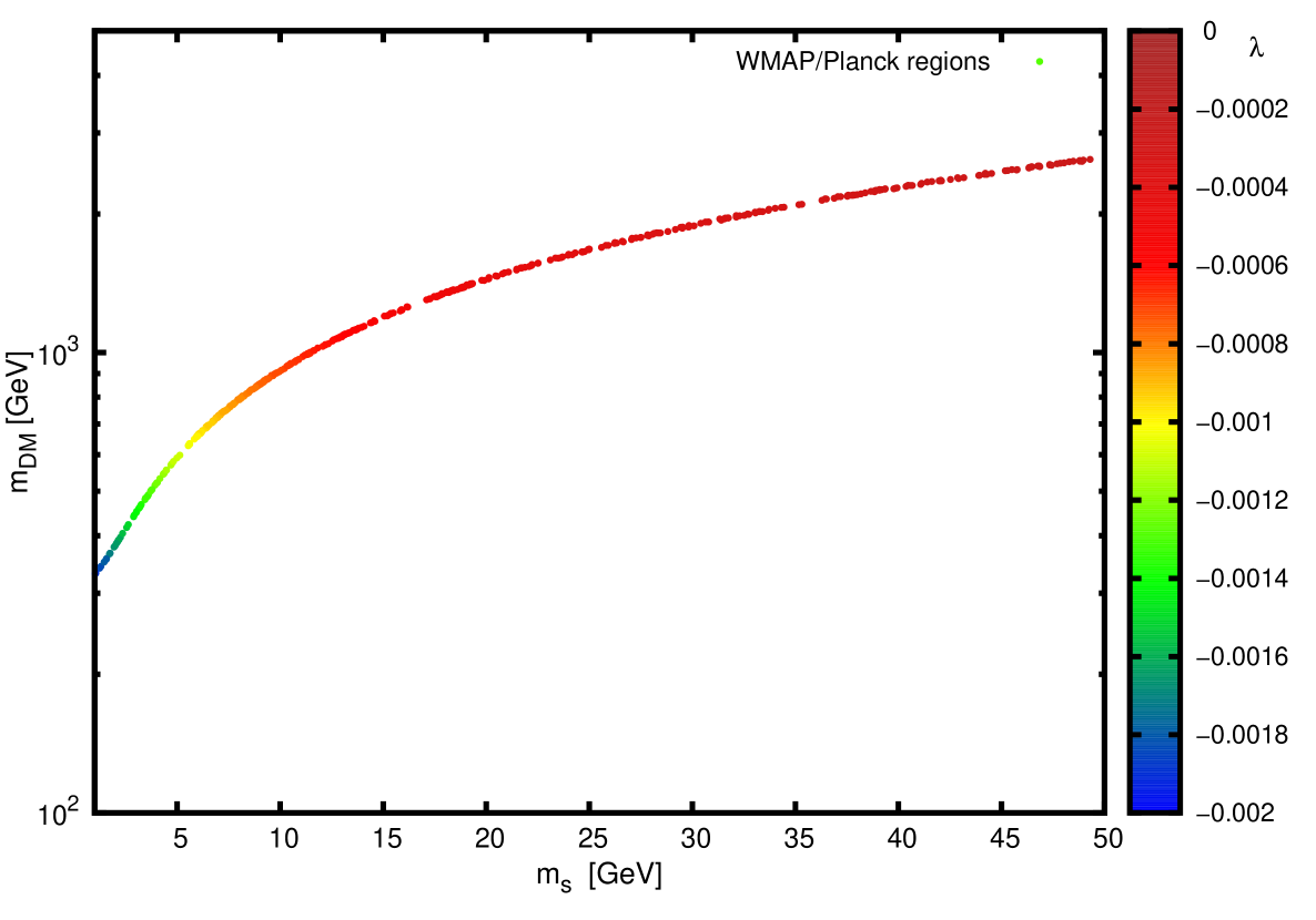
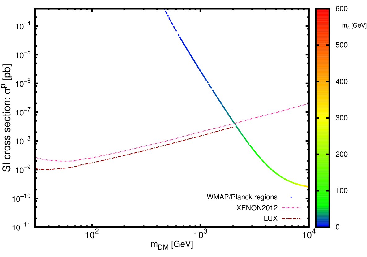
Figure 1: Direct and Indirect probes for single scalar DM in the SISM: Left) The allowed DM mass constrained from DM relic abundance measured by Planck/WMAP against the scalon mass, Right) The allowed DM mass constrained by Planck/WMAP for relic density and by Xenon100/LUX for the elastic scattering cross section of DM off the proton.

We can check our model as well with the direct detection measurements studying the elastic scattering cross section of the dark matter off the nuclei used in the experiments. The scalar DM in our model interacts with the quarks through only the Higgs portal which is a mixing of the scalars $s$ and $h$ here. The Feynman diagram describing the DM-quark interaction $\varphi_{1}q\rightarrow\varphi_{1}q$ is a tree-level diagram drawn in Fig. 5 in Ghorbani:2014gka . The effective potential for such an interaction is given by

$$\mathcal{L}_{\text{eff}}=\alpha_{q}\varphi_{1}\varphi_{1}\bar{q}q\,,$$ (18)

where the effective coupling $\alpha_{q}$ is

$$\alpha_{q}=m_{q}\frac{2\lambda_{H}\lambda_{1}}{\lambda_{H}-\lambda}(\frac{1}{m_{s}^{2}}+\frac{1}{m_{H}^{2}})\,.$$ (19)

It is a good approximation if we consider only the zero momentum transfer in the DM-nucleon scattering. In this limit the quark currents are replaced by the nucleonic currents and the spin-independent (SI) elastic scattering cross section reads

$$\sigma_{\text{SI}}^{\text{N}}=\frac{\alpha_{N}^{2}\mu_{N}^{2}}{\pi m_{\text{DM}}^{2}}\,,$$ (20)

where $\alpha_{N}$ is a factor depending on the effective coupling in eq. (18), the mass of the quarks, the quarks scalar form factors, and the mass of the nucleon which e.g. in the Xenon experiments is the xenon mass (see for instance Ellis:2008hf ; Belanger:2008sj ; Crivellin:2013ipa for more details). We have calculated such elastic scattering for the parameter space which is already restricted by the relic density bounds imposed by Planck and WMAP. Despite the very narrow parameter space we deal with in the current model we observe that still for dark matter masses heavier than around $2$ TeV we have a viable parameter space that respect both the Planck and the Xenon100 bounds. In fact for $m_{\text{DM}}\gtrsim 2$ TeV not only the the bounds by LUX and Xenon100 are respected but even the forthcoming bounds by Xenon1T might not exclude the model. This result is obvious from the right plot in Fig. 1. We should emphasize the role of the non-zero although small scalon mass, in obtaining acceptable results for an only 2-dimensional shrieked parameter space. It is clearly seen from the right panel in Fig. 1 that when the scalon mass goes to zero the scattering cross section grows very fast. A small change to scalon mass from e.g. $0$ to $1$ GeV reduces the cross section for about $15$ orders of magnitudes!

3.2 Two-component Dark Matter

Now in addition to scalars $h$ and $s$ we consider two scalars $\varphi_{1}$ and $\varphi_{2}$ as DM particles with again vanishing vev. This will be a two-component example of dark matter models. The set of parameters are enlarged compared to that of single scalar dark matter and is $\{\lambda_{H},\lambda,\lambda_{s},\lambda_{1},\lambda_{2},\lambda_{\varphi_{1}},\lambda_{\varphi_{2}},\alpha,v_{s}^{2}\}$. The independent parameters that inter in the calculations are the set $\{\lambda,\lambda_{1},\lambda_{2}\}$. Notice that both DM particles $\varphi_{1}$ and $\varphi_{2}$ are stable; non of them decays into the other or to SM particles. The time evolution of each DM scalar is evaluated by two independent Boltzmann equations,

$$\frac{dn_{\varphi_{1}}}{dt}=-3Hn_{\varphi_{1}}-\braket{\sigma^{11}_{\text{ann}}v^{11}_{\text{rel}}}\left[n_{\varphi_{1}}^{2}-\left(n^{\text{eq}}_{\varphi_{1}}\right)^{2}\right]\,,$$ (21)

$$\frac{dn_{\varphi_{2}}}{dt}=-3Hn_{\varphi_{2}}-\braket{\sigma^{22}_{\text{ann}}v^{22}_{\text{rel}}}\left[n_{\varphi_{2}}^{2}-\left(n^{\text{eq}}_{\varphi_{2}}\right)^{2}\right]\,,$$ (22)

where the superscripts $11$ and $22$ in annihilation cross sections mean the cross section for $\varphi_{i}\varphi_{i}\rightarrow SM$ for $i=1,2$ respectively. The allowed region of the space of parameters that must be used in solving the Boltzmann equations (21) and (22) are $-0.128<\lambda<0$, $\lambda_{H}=\lambda+0.128$ and $\lambda_{i}>-1.65\lambda/\lambda_{H}$ for $i=1,2$.

The results of the numerical computation for the relic density and the DM elastic scattering cross section for two-component scalar dark matter are shown in Fig. 2. In the right plot of Fig. 2 the allowed DM masses in the viable parameter space of the relic abundance measured by Planck is drawn against the mediator mass. The behavior observed in the single scalar DM case is not the same as the two-component DM model, i.e. growing the scalon mass does not leads necessarily to greater DM mass. In the right plot in Fig. 2 the viable parameter space which evades both relic and direct constraints are shown, We can see a big change in the range of the DM mass compared to that of the single DM case analyzed in subsection 3.1. The bound for the mass of each scalar DM now is lowered to $m_{\text{DM}}\gtrsim 300$ GeV. Again the non-vanishing scalon mass plays an important role in obtaining a viable parameter space. In Fig. 3 we have shown how the DM mass and the associated DM-nuclei cross sections constrained by the direct and indirect bounds change with respect to the coupling $\lambda_{1}$ instead of the coupling $\lambda$ in both single and two-component DM scenarios. In the two-component case, the dependency of the elastic scattering cross section on the coupling $\lambda_{2}$ is the same as the coupling $\lambda_{1}$, so we refrain drawing a separate plot for that.

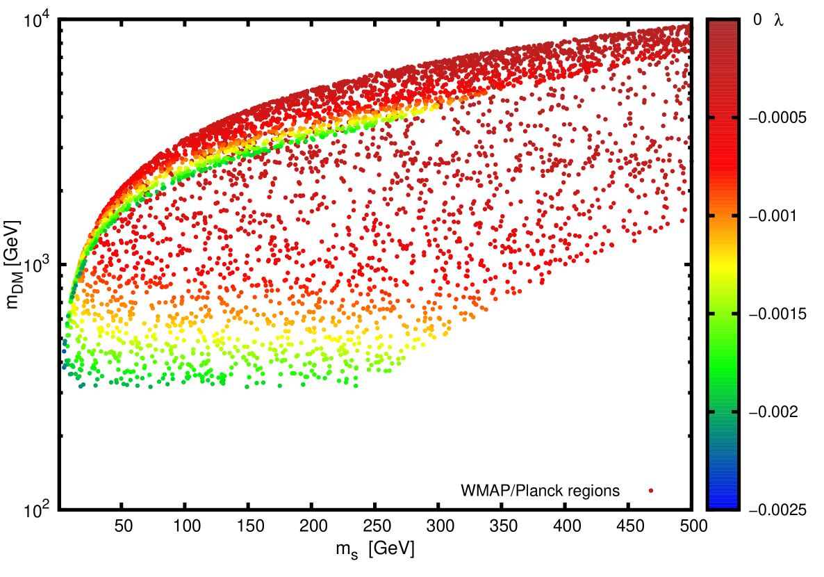
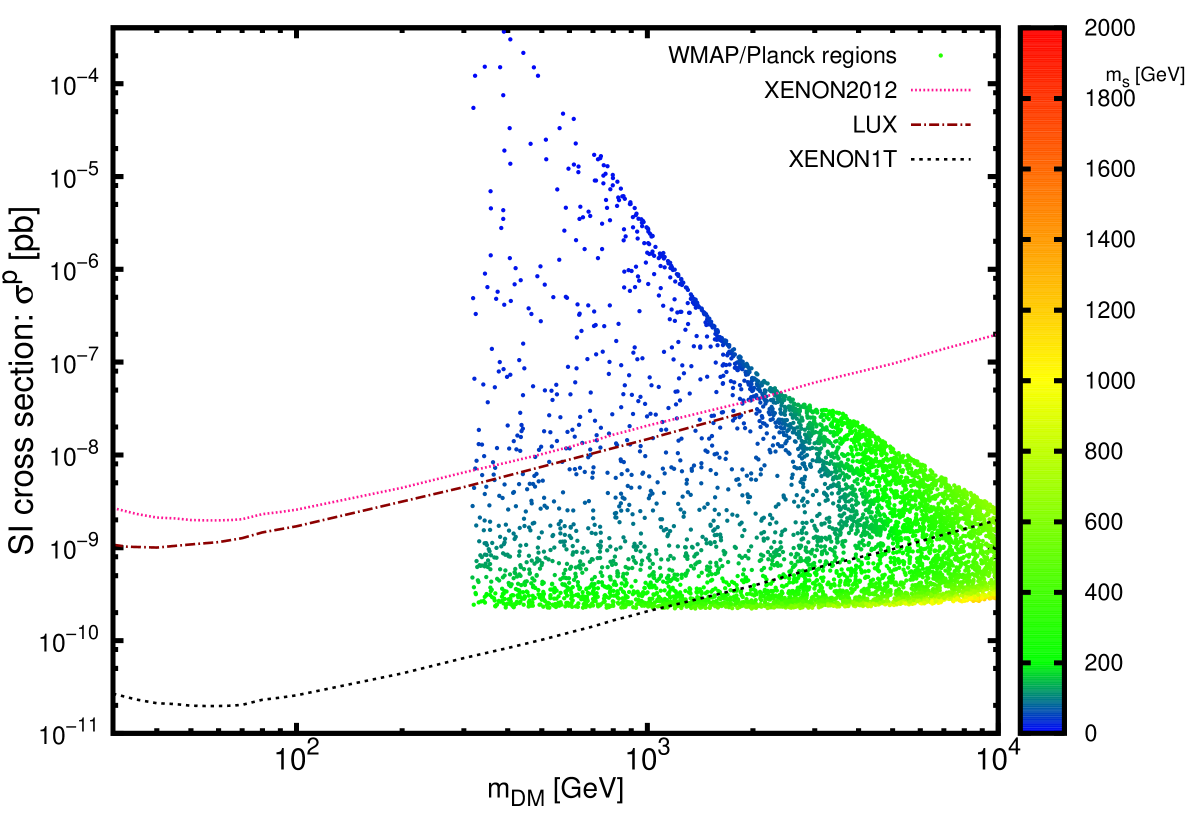
Figure 2: Direct and Indirect probes for two-component scalar DM in the SISM: Left) The allowed DM mass constrained from DM relic abundance measured by Planck/WMAP against the scalon mass, Right) The allowed DM mass constrained by Planck/WMAP for relic density and by Xenon100/LUX for the elastic scattering cross section of DM off the proton.

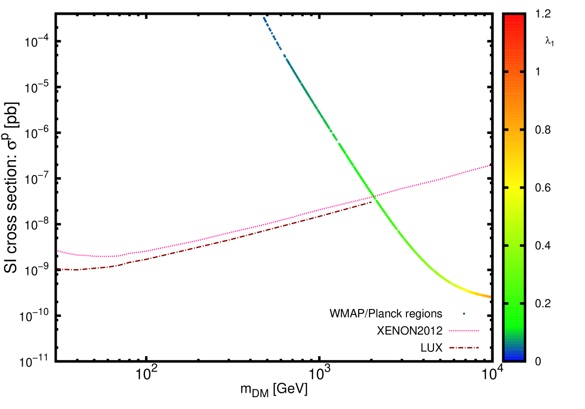
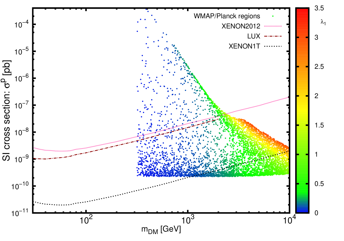
Figure 3: The $\lambda_{1}$ dependency of the allowed DM mass constrained by Planck/WMAP for relic density and by Xenon100/LUX for the elastic scattering cross section of DM off the proton. left) signle dark matter right) two-component dark matter.

3.3 Interacting Dark Matter Components

In the last section the two DM candidates did not have any interaction among themselves. Here we assume an interaction between DM components which respect the scale invariance in the potential (2),

$$V_{\text{int}}=\frac{1}{2}\lambda_{\text{int}}\varphi_{1}^{2}\varphi_{2}^{2}\,.$$ (23)

In our calculations we find out that the presence of the new interacting term (23) does not affect significantly the relic density. More precisely, to see the effect of the coupling $\lambda_{\text{int}}$ we fix all the couplings in the full lagrangian and change $\lambda_{\text{int}}$ in the interval $-3<\lambda_{\text{int}}<3$. We observe that the changes in the amount of relic density compared to when we set $\lambda_{\text{int}}=0$ is at most about $\%0.3$ in the Planck/WMAP region.

4 Discussion

The minimal supersymmetry standard model is capable of addressing some important drawbacks in the standard model such as the Higgs hierarchy problem and the issue of dark matter. However MSSM due to possessing many free parameters is very difficult to be detected experimentally as at LHC no evidence for such a theory has been recorded so far. Motivated by this fact we are interested in studying the scale invariant standard model (massless-Higgs standard model) which is free of hierarchy problem. In SISM the Higgs boson receives mass from the vacuum expectation value of another scalar called scalon which remains massless classically. However radiative corrections gives a small mass to the scalon that is crucial if we want to extend this theory to include DM candidates. More scalars in the theory then can play the role of DM particle(s). By adding once one scalar and then two scalars we have considered the case of single scalar dark matter and two component dark matter in SISM. In this paper we have examined the SISM whether it can accommodate the problem of dark matter as a WIPM in the freeze-out scenario. We observed remarkably that the SISM despite having a narrow parameter space already restricted due to the scale invariance is quite successful in overcoming the constraints dark matter relic abundance and the direct detection of dark matter elastic scattering of nuclei, far enough below the bounds put by Planck and Xenon100 as seen from Figs. 1 and 2.

In the following we discuss briefly the case in which the SISM is extended by a fermionic DM candidate. Suppose in addition to Higgs scalar $h$ and the scalon $s$ the theory possesses a Dirac fermion that is communicating with the SM sector through the Higgs portal by a Yukawa interaction,

$$\mathcal{L}_{\text{int}}=gs\bar{\psi}\psi+g_{5}s\bar{\psi}\gamma^{5}\psi\,,$$ (24)

where $g$ and $g_{5}$ are the Yukawa couplings. The coefficients in the effective potential (10) in the absence of any DM scalars gets contribution from the fermion DM in the loop,

$$\begin{split}A(\bar{\mathbf{n}})=\frac{1}{64\pi^{2}v_{\phi}^{2}}\bigg{[}m_{h}^{4}\left(-\frac{2}{3}+\log{\frac{m_{h}^{2}}{v_{\phi}^{2}}}\right)+6m_{W}^{4}\left(-\frac{5}{6}+\log{\frac{m_{W}^{2}}{v_{\phi}^{2}}}\right)+3m_{Z}^{4}\left(-\frac{5}{6}+\log{\frac{m_{Z}^{2}}{v_{\phi}^{2}}}\right)\\ -12m_{t}^{4}\left(-1+\log{\frac{m_{t}^{2}}{v_{\phi}^{2}}}\right)-4m_{\psi}^{4}\left(-1+\log{\frac{m_{\psi}^{2}}{v_{\phi}^{2}}}\right)\bigg{]}\,,\end{split}$$ (25)

and

$$B(\bar{\mathbf{n}})=\frac{1}{64\pi^{2}v_{\phi}^{4}}\left(m_{h}^{4}+6m_{W}^{4}+3m_{Z}^{4}-12m_{t}^{4}-4m_{\psi}^{4}\right)\,.$$ (26)

The mass of the scalon then takes the form

$$\delta m_{s}^{2}=2Bv_{\phi}^{2}=-\frac{\lambda}{32\pi^{2}m_{H}^{2}}\left(m_{H}^{4}+6m_{W}^{4}+3m_{Z}^{4}-12m_{t}^{4}-4m_{\psi}^{4}\right)\,.$$ (27)

The coupling $\lambda$ takes only negative values as pointed out in section 3. It should be noted first that even before adding the DM fermion the scalon mass correction becomes negative due to the existence of the heavy top quark in the loop. So the presence of the DM fermion deteriorates the situation. In addition to Higgs scalar and the scalon, it is therefore necessary to add more bosons (scalars or vector bosons) to the theory. In the presence of further bosons the issue of fermionic DM in SISM is at least consistent by construction (see Benic:2014aga for an example). However the positivity of the scalon mass restricts strongly the mass of the Dirac fermion $\psi$ and the scalon $s$ remains always very light, which in turn as discussed in subsection 3.1 the theory might be ruled out by constraints from direct detection tests.

References

- (1) S. Weinberg, Implications of Dynamical Symmetry Breaking, Phys. Rev. D13 (1976) 974–996.
- (2) E. Gildener, Gauge Symmetry Hierarchies, Phys. Rev. D14 (1976) 1667.
- (3) Planck collaboration, R. Adam et al., Planck 2015 results. I. Overview of products and scientific results, 1502.01582.
- (4) WMAP collaboration, G. Hinshaw et al., Nine-year wilkinson microwave anisotropy probe (wmap) observations: Cosmological parameter results, Astrophys.J.Suppl. 208 (2013) 19, [1212.5226].
- (5) P. Gondolo, J. Edsjo, P. Ullio, L. Bergstrom, M. Schelke and E. A. Baltz, DarkSUSY: Computing supersymmetric dark matter properties numerically, JCAP 0407 (2004) 008, [astro-ph/0406204].
- (6) G. Jungman, M. Kamionkowski and K. Griest, Supersymmetric dark matter, Phys. Rept. 267 (1996) 195–373, [hep-ph/9506380].
- (7) P. Brax, A.-C. Davis and H. A. Winther, Cosmological supersymmetric model of dark energy, Phys. Rev. D85 (2012) 083512, [1112.3676].
- (8) ATLAS collaboration, G. Aad et al., Summary of the ATLAS experiment’s sensitivity to supersymmetry after LHC Run 1 — interpreted in the phenomenological MSSM, JHEP 10 (2015) 134, [1508.06608].
- (9) CMS collaboration, V. Khachatryan et al., Search for supersymmetry with photons in pp collisions.., Phys. Rev. D92 (2015) 072006, [1507.02898].
- (10) K. A. Meissner and H. Nicolai, Conformal Symmetry and the Standard Model, Phys. Lett. B648 (2007) 312–317, [hep-th/0612165].
- (11) R. Foot, A. Kobakhidze, K. L. McDonald and R. R. Volkas, A Solution to the hierarchy problem from an almost decoupled hidden sector within a classically scale invariant theory, Phys. Rev. D77 (2008) 035006, [0709.2750].
- (12) S. R. Coleman and E. J. Weinberg, Radiative Corrections as the Origin of Spontaneous Symmetry Breaking, Phys. Rev. D7 (1973) 1888–1910.
- (13) E. Gildener and S. Weinberg, Symmetry Breaking and Scalar Bosons, Phys. Rev. D13 (1976) 3333.
- (14) J. Guo and Z. Kang, Higgs Naturalness and Dark Matter Stability by Scale Invariance, Nucl. Phys. B898 (2015) 415–430, [1401.5609].
- (15) A. Karam and K. Tamvakis, Dark matter and neutrino masses from a scale-invariant multi-Higgs portal, Phys. Rev. D92 (2015) 075010, [1508.03031].
- (16) G. Belanger, F. Boudjema, A. Pukhov and A. Semenov, micrOMEGAs3: A program for calculating dark matter observables, Comput. Phys. Commun. 185 (2014) 960–985, [1305.0237].
- (17) G. Bélanger, F. Boudjema, A. Pukhov and A. Semenov, micrOMEGAs4.1: two dark matter candidates, Comput. Phys. Commun. 192 (2015) 322–329, [1407.6129].
- (18) S. Dodelson, Modern Cosmology. Academic Press, Amsterdam, 2003.
- (19) K. Ghorbani and H. Ghorbani, Two-portal Dark Matter, Phys. Rev. D91 (2015) 123541, [1504.03610].
- (20) K. Ghorbani and H. Ghorbani, Scalar Split WIMPs in the Future Direct Detection Experiments, 1501.00206.
- (21) J. R. Ellis, K. A. Olive and C. Savage, Hadronic Uncertainties in the Elastic Scattering of Supersymmetric Dark Matter, Phys. Rev. D77 (2008) 065026, [0801.3656].
- (22) G. Belanger, F. Boudjema, A. Pukhov and A. Semenov, Dark matter direct detection rate in a generic model with micrOMEGAs 2.2, Comput. Phys. Commun. 180 (2009) 747–767, [0803.2360].
- (23) A. Crivellin, M. Hoferichter and M. Procura, Accurate evaluation of hadronic uncertainties in spin-independent WIMP-nucleon scattering: Disentangling two- and three-flavor effects, Phys. Rev. D89 (2014) 054021, [1312.4951].
- (24) S. Benic and B. Radovcic, Majorana dark matter in a classically scale invariant model, JHEP 01 (2015) 143, [1409.5776].