Footprints of Loop I on Cosmic Microwave Background Maps

Abstract

Cosmology has made enormous progress through studies of the cosmic microwave background, however the subtle signals being now sought such as $B$-mode polarisation due to primordial gravitational waves are increasingly hard to disentangle from residual Galactic foregrounds in the derived CMB maps. We revisit our finding that on large angular scales there are traces of the nearby old supernova remnant Loop I in the WMAP 9-year map of the CMB and confirm this with the new SMICA map from the Planck satellite.

1 Introduction

We have shown earlier [1] that there is a clear imprint of the Galactic ‘radio Loop I’ [2] on the internal linear combination (ILC) map of the cosmic microwave background (CMB) constructed using multi-frequency data obtained by the Wilkinson Microwave Anisotropy Probe (WMAP) [3]. We interpreted this anomaly [1] as possibly due to magnetic dipole emission (MDE) from magnetised dust grains [4, 5] which can mimic a thermal blackbody like the CMB over a restricted frequency range. However MDE is not an unique mechanism to explain the Loop I anomaly, rather it could be a more complex interplay between various Galactic foreground emissions (viz. free-free, thermal dust and synchrotron) which vary across the sky.

Subsequently it was claimed that our analysis had not correctly selected the hottest peaks in the simulated sky realisations and that it was sensitive to the map pixelization used, such that with a different pixel size, the peak-to-loop angular distance for the highest temperature bins is no longer unusual [6]. Consideration of these effects was stated to reduce the significance of the Loop I–CMB correlation such that the chance probability is as large as $\sim 1\%$ [6], rather than 0.018% [1].

In their recent study of low frequency Galactic foregrounds, the Planck Collaboration [7] add the further concern that the physical structure of Loop I may differ [8] from our modelling of it as a spherical shell of uniform emissivity [2, 9]. They also argue against the anomalous correlated signal being MDE on the grounds that since there should be many more such old supernova remnants (SNRs) in the Galactic plane [9] but no such signal is apparent in the WMAP ILC map.

We demonstrate here with a new statistic which measures the clustering of hot spots along Loop I that our previous significance estimate is in fact robust. We show in addition that the correlation between Loop I and inferred maps of the CMB holds also for the Planck SMICA map [10] and that this is not sensitive to any Galactic mask used. We address the second criticism by presenting additional analyses and explanations below.

2 Mean temperature around Loop I

As reported for the WMAP 9 yr ILC map [3], the average temperature around the Loop I ring is anomalously high and the probability of finding an average temperature at least as high in a $\Lambda$CDM random Gaussian field is $\sim 1\%$ [1]. We repeat the analysis for the 2015 Planck SMICA map [10] and investigate the effect of masking the Galactic plane. (Hereafter we refer to these maps simply as ILC9 and SMICA.)

Since we are interested in a rather diffuse structure, we apply a low–pass filter by limiting the analysis to multipoles $\ell\leq\ell_{\text{max}}=20$ (as justified in § 5). Throughout, we work at a HEALPix [11] resolution of $\text{Nside}=128$ (although the results are much the same at higher resolution because of our $\ell_{\text{max}}=20$ filter). We compute the average temperature $\overline{T}$ in a $\pm 2^{\circ}$ wide band around the Loop I ring — defined as a small circle of diameter $116^{\circ}$ centred at $(l,b)=(329^{\circ},17.5^{\circ})$ [2]. To evaluate the chance probability of an average temperature at least as high, we simulate $10^{4}$ maps with the WMAP 9 yr best–fit angular power spectrum [3]. Both the fraction of simulations with a more extreme average temperature, and the $p$–value of a Gaussian with the mean and standard deviation of the distribution of simulated $\overline{T}$ are determined. We also investigate the effect of applying the standard KQ85 and SMICA masks, having downgraded these to $\text{Nside}=128$.

map	mask	$\overline{T}[\mu\text{K}]$	$p$–value (from SD)	$p$–value (more extreme $\overline{T}$)
ILC9	none	23.9	0.01	0.01
ILC9	KQ85	15.4	0.09	0.09
SMICA	none	22.8	0.01	0.01
SMICA	SMICA	21.8	0.02	0.02

Table 1: The mean temperature around Loop I (and the chance probability) in various CMB maps.

The results are reported in Table 1. We find an anomalously high average temperature of around 20 $\mu$K, for both the ILC9 and SMICA maps. The $p$–values are of order $1\%$, when not applying a mask. For the SMICA map, the $p$–value increases to 2% when the SMICA mask is applied, but the average temperature remains virtually unchanged ($\overline{T}=21.8$ versus $22.8\mu\text{K}$). The increase in the $p$–value is therefore in part due to the increased sample variance when applying the mask, and not solely to masking of residual contamination from the Galactic plane. The agreement between the $p$–values estimated in two separate ways is just as expected for a Gaussian random field.

3 Cross-correlation between temperature and pixel-to-loop distance

Fig. 3 of our paper [1] shows that as the pixel temperature increases, the angular distance between the corresponding pixel and the centre of Loop I decreases, which is a global effect and not just determined by the 4 highest temperature bins. This can be quantified by the cross-correlation between $G(\text{p}_{j})$ and $T(\text{p}_{j})$, where $G(\text{p}_{j})$ is the angular distance (along great circles) between the $j$-th pixel and the centre of Loop I, and $T(\text{p}_{j})$ is the temperature of the $j$-th pixel—both computed with no binning. This cross-correlation coefficient is:

$$C(G,T)=\frac{\sum{(G-\mu_{G})(T-\mu_{T})}}{\sqrt{\sum{(G-\mu_{G})^{2}}\sum{(T-\mu_{T})^{2}}}},$$ (3.1)

where $\mu_{T}$ and $\mu_{G}$ are the sample average of $T$ and $G$ in the Loop I region. Using the low–pass filter with $\ell_{\text{max}}=20$ we find $C(G,T)=-0.22$ for the ILC9 map and $C(G,T)=-0.20$ for the SMICA map. As above, this result is insensitive to the map’s resolution. In addition, via its definition (3.1), the cross-correlation is affected only by relative deviations from the mean, and not the absolute amplitude. Both of these findings counter the criticism  [6] of our work, viz. the alleged sensitivity to the map pixelisation and the insensitivity of the method towards possibly hotter peaks in the simulations.

By generating $10^{4}$ simulations based on the best-fit $\Lambda$CDM model power spectrum, we estimate the significance of finding $C(G,T)=-0.22$ (for the ILC9 map) to be $\sim 4\times 10^{-4}$ and $C(G,T)=-0.20$ (for the SMICA map) to be $\sim 10^{-3}$. Again, the distribution of $C(G,T)$ is well-fitted by a Gaussian (see Fig. 1) and both $p$–values are comparable to our earlier result [1]. Hence our claim that there is a $\sim 24\mu$K anomalous signal from Loop I which has somehow evaded standard foreground cleaning techniques, does stand up to detailed scrutiny.

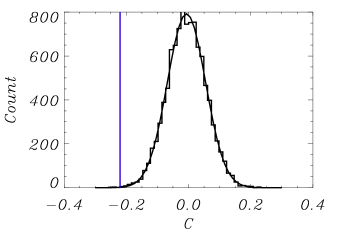
Figure 1: The histogram of $C(G,T)$ for $10^{4}$ simulations. The blue line indicates the value obtained from ILC9.

4 Can the Loop I anomaly be removed by masking?

It has been suggested [6, 7] that the anomaly in the Loop I region is not due to unsubtracted intrinsic emission from Loop I but rather contamination from other regions in the Galactic plane along the line-of-sight. However if this were so, one would not in general expect the hot spots inside the Galactic plane mask to correlate with the Loop I ring. If this happens by chance, the anti–correlation ($C(G,T)<0$) would be weaker when the Galactic mask is applied. However we find that $C(G,T)$ is unaffected by the masks.

To check the effect of masking we reexamine the hot spots in the SMICA map smoothed with $\ell_{\text{max}}=20$ using 4 different masks: SMICA, Commander, NILC and SEVEM [10]. In Fig. 2 we mark the boundary of the masks with black lines and indicate local maxima along Loop I in the CMB temperature with black circles. It can be seen that most of the local maxima lie outside the masks. Unsurprisingly, the value of $C(G,T)$ is nearly independent of the mask, or the resolution of the CMB map. This is exhibited in Table 2 along with the corresponding significances from $10^{4}$ simulations.

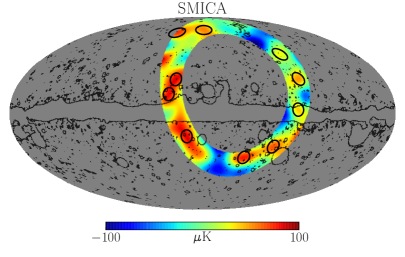
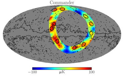
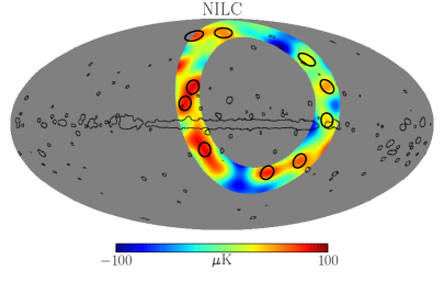
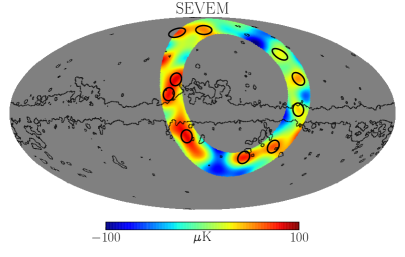
Figure 2: The positions of local maxima of the temperature (black circles) along Loop I relative to SMICA, Commander, NILC and SEVEM masks (black lines).

map	mask	$C(G,T)$	$p$–value (from std. dev.)	$p$–value (more extreme $C(G,T)$)
ILC9	none	-0.22	$3.9\times 10^{-4}$	$7.0\times 10^{-4}$
ILC9	KQ85	-0.17	$1.4\times 10^{-2}$	$1.5\times 10^{-2}$
SMICA	none	-0.20	$9.8\times 10^{-4}$	$1.4\times 10^{-3}$
SMICA	SMICA	-0.20	$2.0\times 10^{-3}$	$2.6\times 10^{-3}$
SMICA	Commander	-0.20	$2.8\times 10^{-3}$	$3.8\times 10^{-3}$
SMICA	NILC	-0.20	$1.2\times 10^{-3}$	$1.7\times 10^{-3}$
SMICA	SEVEM	-0.20	$2.1\times 10^{-3}$	$2.4\times 10^{-3}$

Table 2: The temperature-angular distance correlation at $\text{Nside}=128$. We quote the correlation coefficient $C(G,T)$, the $p$–value (assuming a Gaussian distribution of simulated $C(G,T)$’s) and the fraction of simulations with smaller $C(G,T)$’s for different CMB maps and masks.

5 Justification of the low-pass filter scale

We now explain the choice of $\ell_{\text{max}}=20$ for filtering the CMB map used in our previous [1] as well as this work, by comparing the angular width of Loop I with the characteristic correlation angle $\theta_{\text{c}}$ from the CMB maps. These ought to be comparable if we wish to find a correlated signal between the two. The correlation angle $\theta_{\text{c}}$ is defined using the two-point correlation function $C(\theta)$ as:

$$C(\theta)\simeq C(0)+\frac{1}{2}C^{\prime\prime}(0)\theta^{2}+\ldots\simeq C(0)\left(1-\frac{1}{2}\frac{\theta^{2}}{\theta_{\text{c}}^{2}}\right)$$ (5.1)

where the primes indicate differentiation with respect to $\theta$. Hence

$$\theta_{\text{c}}^{2}\equiv-\frac{C(0)}{C^{\prime\prime}(0)}=\frac{2\sum_{\ell=2}^{\ell_{\text{max}}}(2\ell+1)C_{\ell}}{\sum_{\ell=2}^{\ell_{\text{max}}}(2\ell+1)(\ell+1)\ell C_{\ell}}$$ (5.2)

clearly depends on the choice of $\ell_{\text{max}}$. In addition to a sharp cutoff at $\ell_{\text{max}}$ we also consider a smooth cutoff $\propto\exp(-\ell^{2}/\ell^{2}_{\text{max}})$ in the sums above and let $\widetilde{\theta}_{\text{c}}$ denote the corresponding correlation angle. We calculate these for different $\ell_{\text{max}}$ in the range 10–40 using the best-fit $\Lambda$CDM cosmology and power spectra from the SMICA and ILC9 maps as shown in Fig. 3. The correlation angles for $\ell_{\text{max}}=20$ all lie around $8^{\circ}$ (see Table 3).

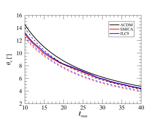
Figure 3: Correlation angles $\theta_{\text{c}}$ (solid) and $\widetilde{\theta}_{\text{c}}$ (dashed) versus $\ell_{\text{max}}$, for the SMICA and ILC9 maps.

	$\text{Nside}=512$		$\text{Nside}=16$
	$\theta_{c}$	$\widetilde{\theta_{c}}$	$\theta_{c}$	$\widetilde{\theta_{c}}$
$\Lambda\text{CDM}$	$8.77^{\circ}$	$8.26^{\circ}$	$8.77^{\circ}$	$8.35^{\circ}$
ILC9	$8.28^{\circ}$	$7.73^{\circ}$	$8.46^{\circ}$	$8.41^{\circ}$
SMICA	$8.19^{\circ}$	$7.59^{\circ}$	$8.33^{\circ}$	$8.22^{\circ}$

Table 3: Values of $\theta_{c}$ and $\widetilde{\theta_{c}}$ for $\ell_{\text{max}}=20$ at $\text{Nside}=512$ and $16$.

Observations [13] of Loop I are well-fitted by modelling it as a shell of uniform emissivity [9] as seen in the left panel of Fig. 4. We calculate the full width at half maximum (FWHM) and find this to be $\theta_{\text{FWHM}}=6.6^{\circ}$ if the zero-level is taken to be at the centre. However there is emission above the background even here — had we chosen the zero-level outside of the loop the resulting $\theta_{\text{FWHM}}$ would be $10.9^{\circ}$, marked in red in the left panel of Fig. 4. The angular width of Loop I is thus comparable to the correlation angle for $\ell_{\text{max}}=20$, justifying this as our choice [1] for smoothing the CMB maps.

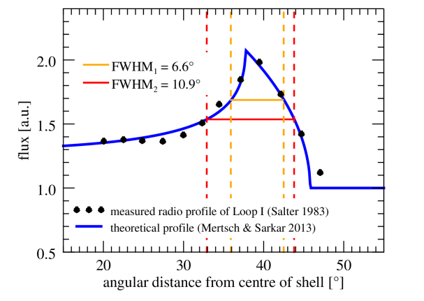
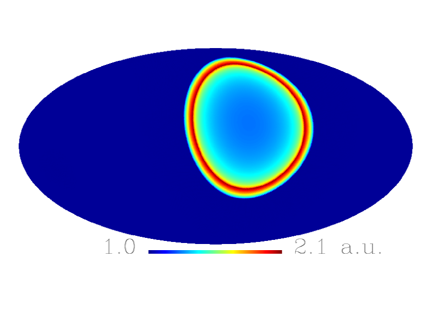
Figure 4: The modelled angular profile of Loop I [9] with the FWHM defined by two different measures (zero-level at centre or outside the loop) marked in orange and red, respectively, and its projection on the sky.

The power spectra used above were obtained from maps using $\text{Nside}=512$. We expect these results to hold for lower resolutions as well, as the angular power does not change much below the value for $\ell_{\text{max}}$ considered here. To illustrate this, we show in the same Table 3 values obtained from maps at $\text{Nside}=16$ which differ very little from the values obtained at higher resolution.

6 Should anomalous emission be seen from other loops?

The presence of a foreground residual that is morphologically correlated with a well known Galactic structure, viz. Loop I, demonstrates the limitations of conventional (frequency–based) foreground cleaning techniques. We had sugested [1] that this residual is harder than synchrotron but also softer than electric dipole emission from thermal dust, so may have a near blackbody spectrum as expected of magnetic dipole emission from magnetised dust [5]. Such a previously unrecognised (see however [4]) foreground would understandably pose a serious challenge for separating the CMB signal—in the absence of any tracer map of MDE.

As mentioned, the Planck Collaboration [7] have argued that if MDE is the cause of the contamination in the Loop I region, such emission should have been observed from the Galactic disk which harbours thousands of such old SNRs (‘all loops’) [9]. We have checked this by using our simulation of radio emission from the 4 known radio loops (including Loop I) and the Galactic population of old SNRs, using the same simulated maps as shown in the middle row of Fig. 11 of Ref. [9]. In Fig. 5 we show the latitudinal profiles of the column density through the Galactic population of all loops (both the average and the maximum) in the longitude intervals $[-180^{\circ},180^{\circ}]$ (left panel) and $[-60^{\circ},60^{\circ}]$ (right panel). These are compared with a slice through Loop I at longitude $=0^{\circ}$.

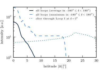
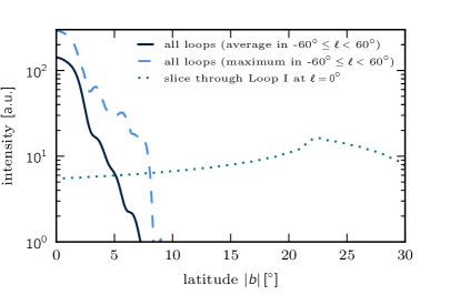
Figure 5: Latitudinal profiles of the column density through the Galactic population of all loops in the longitude intervals indicated, compared to a slice through Loop I.

It is seen that up to $|b|\sim 5^{\circ}$, the average contribution from all Galactic loops dominates over the contribution from Loop I. At higher latitude, however, the intensity of Loop I is higher and peaks at $b=-22^{\circ}$ (for the $l=0^{\circ}$ slice). The maximum of all Galactic loops in the longitude interval $[-180^{\circ},180^{\circ}]$ is almost constant for latitude $(8-18)^{\circ}$ where sight lines intersect with at most one loop. At larger distances, the line of sight does not cross any Galactic loops due to the excision in the simulation of heliocentric distances $<500$ pc (in order to avoid double counting of local shells). For the longitude interval $[-60^{\circ},60^{\circ}]$ this drop happens at even smaller latitude; due to the position of the Solar system with respect to the nearest spiral arm, the closest (and therefore spatially most extended) Galactic loops are in the second and third Galactic quadrant (i.e. outside the interval $[-60^{\circ},60^{\circ}]$).

In this analysis we have likely overestimated the column–depth for the Galactic loops (or underestimated that of Loop I). This is because we have worked directly from the simulated synchrotron maps and the synchrotron emissivity of the loops is higher in the inner Galaxy where cosmic ray electron density and the magnetic field strength are larger. Dust emission, on the other hand, does not depend on these variables hence the intensity from all loops close to the disk is likely smaller than shown in Fig. 5, making the band where it dominates over Loop I even narrower.

Thus we can conservatively conclude that the column density through Galactic loops dominates over that of Loop I only in a narrow band around the Galactic plane, $|b|\lesssim 5^{\circ}$ (possibly even smaller). It is our understanding that the presence of MDE in this region cannot be excluded since component separation methods are least effective here (cf. the Galactic masks shown in Fig. 2). Moreover in the disk this emission necessarily correlates with free–free emission: the distribution of SNRs closely follows the free electron density and therefore the map of the average column depth through old loops should be similar to the free–free map. Given this morphological similarity, in supposedly foreground–cleaned CMB maps like ILC or SMICA, part of the MDE may have been misidentified as free–free emission, and perhaps even labelled as the ‘anomalous microwave emission’ which is seen to correlate with free–free emission [7]. We shall present a study of such possibilities elsewhere.

7 Summary

We have revisited the issue of a $\sim 20\mu\text{K}$ excess in the Loop I region discovered [1] in the WMAP ILC9 map and have detected its presence in the 2015 Planck SMICA map as well. We have presented an improved test statistic for investigating the clustering of hot spots around Loop I, confirming such clustering for the ILC9 and SMICA map of the same order as was originally claimed. We have found that even when the usual temperature analysis masks are applied the anomaly still persists; for the SMICA map all four analysis masks (SMICA, Commander, NILC and SEVEM) lead to $p$–values of ${\cal O}(10^{-3})$. Additionally we provide a justification of the low-pass filter scale ($\ell_{\text{max}}=20$) used, based on the observed width of the radio profile of Loop I. Finally, we show that the similar anomalous emission that might be expected from other old supernova remnants in the Galaxy is confined to a narrow band along the Galactic plane and hence may not have been identified as such. Polarisation maps from Planck will be essential to make further progress in understanding this important foreground for the CMB, especially at high galactic latitude.

References

- [1] H. Liu, P. Mertsch and S. Sarkar, Astrophys. J. 789 (2014) L29 [arXiv:1404.1899 [astro-ph.CO]].
- [2] E. M. Berkhuijsen, C. G. T. Haslam and C. J. Salter, Astron. Astrophys. 14 (1971) 252
- [3] C. L. Bennett et al. [WMAP Collaboration], Astrophys. J. Suppl. 208 (2013) 20 [arXiv:1212.5225 [astro-ph.CO]].
- [4] B. T. Draine and B. Hensley, Astrophys. J. 757 (2012) 103 [arXiv:1205.6810 [astro-ph.GA]].
- [5] B. T. Draine and B. Hensley, Astrophys. J. 765 (2013) 159 [arXiv:1205.7021 [astro-ph.GA]].
- [6] R. W. Ogburn, arXiv:1409.7354 [astro-ph.CO].
- [7] P. A. R. Ade et al. [Planck Collaboration], arXiv:1506.06660 [astro-ph.GA].
- [8] M. Vidal, C. Dickinson, R. D. Davies and J. P. Leahy, Mon. Not. Roy. Astron. Soc. 452 (2015) 1, 656 [arXiv:1410.4438 [astro-ph.GA]].
- [9] P. Mertsch and S. Sarkar, JCAP 1306 (2013) 041 [arXiv:1304.1078 [astro-ph.GA]].
- [10] R. Adam et al. [Planck Collaboration], arXiv:1502.05956 [astro-ph.CO].
- [11] K. M. Gorski, E. Hivon, A. J. Banday, B. D. Wandelt, F. K. Hansen, M. Reinecke and M. Bartelman, Astrophys. J. 622 (2005) 759 [astro-ph/0409513]. http://healpix.sourceforge.net
- [12] http://lambda.gsfc.nasa.gov/product/map/dr5/ilc_map_info.cfm
- [13] C. J. Salter, Bull. Astron. Soc. India 11 (1983) 1
- [14] http://www.cosmos.esa.int/web/planck