Passive scalar mixing and decay at finite correlation times in the Batchelor regime

Abstract

An elegant model for passive scalar mixing and decay was given by Kraichnan (1968) assuming the velocity to be delta-correlated in time. For realistic random flows this assumption becomes invalid. We generalize the Kraichnan model to include the effects of a finite correlation time, $\tau$, using renewing flows. The generalized evolution equation for the 3-D passive scalar spectrum $\hat{M}(k,t)$ or its correlation function $M(r,t)$, gives the Kraichnan equation when $\tau\to 0$, and extends it to the next order in $\tau$. It involves third and fourth order derivatives of $M$ or $\hat{M}$ (in the high $k$ limit). For small-$\tau$ (or small Kubo number), it can be recast using the Landau-Lifshitz approach, to one with at most second derivatives of $\hat{M}$. We present both a scaling solution to this equation neglecting diffusion and a more exact solution including diffusive effects. To leading order in $\tau$, we first show that the steady state 1-D passive scalar spectrum, preserves the Batchelor (1959) form, $E_{\theta}(k)\propto k^{-1}$, in the viscous-convective limit, independent of $\tau$. This result can also be obtained in a general manner using Lagrangian methods. Interestingly, in the absence of sources, when passive scalar fluctuations decay, we show that the spectrum in the Batchelor regime and at late times, is of the form $E_{\theta}(k)\propto k^{1/2}$ and also independent of $\tau$. More generally, finite $\tau$ does not qualitatively change the shape of the spectrum during decay. The decay rate is however reduced for finite $\tau$. We also present results from high resolution ($1024^{3}$) direct numerical simulations of passive scalar mixing and decay. We find reasonable agreement with predictions of the Batchelor spectrum, during steady state. The scalar spectrum during decay is however dependent on initial conditions. It agrees qualitatively with analytic predictions when power is dominantly in wavenumbers corresponding to the Batchelor regime, but is shallower when box scale fluctuations dominate during decay.

1 Introduction

Understanding turbulent mixing and decay of passive scalars is important in a number of natural settings, for many practical applications and also as a means to get insight into turbulence itself (Shraiman & Siggia, 2000; Warhaft, 2000; Sreenivasan & Schumacher, 2010; Davidson et al., 2013). These settings and applications include atmospheric phenomena, oceanography, combustion, dispersion of pollutants, transport of heat and even metal mixing in the interstellar medium of galaxies. Progress in understanding passive scalar turbulence may also ultimately lead to a better understanding of fluid turbulence itself, as it offers a simpler setting wherein many of the issues of fluid turbulence can be examined.

The spectrum of passive scalar fluctuations advected by a turbulent or random flow has received attention right from the early days of turbulence research (Obukhov, 1949; Corrsin, 1951; Batchelor, 1959; Kraichnan, 1968). This spectrum depends on the relative importance of the viscous dissipation (as characterised by the kinematic viscosity $\nu$) compared to the scalar diffusivity ($\kappa$). If the fluid Reynolds number, $\mbox{\rm Re}=u/(k_{f}\nu)$ is large such that there is an extensive inertial range for the turbulent velocity, and the corresponding Peclet number $\mbox{\rm R}_{\kappa}=u/(k_{f}\kappa)$ is also comparable, the one dimensional scalar spectrum is expected to scale as, $E_{\theta}(k)\propto k^{-5/3}$, the same form as the Kolmogorov spectrum for the velocity (Obukhov, 1949; Corrsin, 1951; Batchelor, 1959). Here $u$ and $k_{f}$ are characteristic velocity and wavenumber where the fluid is driven in some random fashion. This range of wavenumbers is referred to as the inertial-convective range, where the velocity fluctuations belong to the inertial range and convect the passive scalar.

Another interesting regime, often referred to as the viscous-convective or the Batchelor regime, obtains when the Schmidt number $Sc=\nu/\kappa\gg 1$ (or the thermal Prandtl number when the passive scalar is temperature). In this case the viscous cut-off scale is much larger than that due to the scalar diffusion; or the corresponding viscous cut-off wavenumber $k_{\nu}\ll k_{\kappa}$, the cut-off wavenumber corresponding to the scalar fluctuations. The velocity field below the viscous scale is smooth and thus the scalar mixing in this regime is dominated by the random shearing by relatively smooth viscous scale eddies.

The resulting passive scalar spectrum was analysed by Batchelor (1959) (B59), based on the effect of linear shear flows on the scalar density. For an incompressible velocity ${\bf u}$, a given scalar blob is eventually stretched along one direction and compressed along the direction of the maximally negative strain. B59 assumed that the principal axes of the flow are random and isotropically distributed, but the magnitudes of the strains are fixed. On averaging over the directions of these principal axes, B59 then argued that the steady state 1-D scalar spectrum $E_{\theta}(k)\propto 1/k$, for $k_{\nu}\ll k\ll k_{\kappa}$. In the above analysis, the randomness in time of the velocity field, that it has a finite correlation time in a realistic turbulent flow, was not explicitly taken into account.

Kraichnan (1968) (K68) re-examined the problem of passive scalar mixing and decay in the opposite extreme case of a delta-correlated in time velocity field. This assumption of delta-correlation, allows one to convert the stochastic differential equation for the passive scalar, to a partial differential equation in real space for the time evolution of the scalar correlation function $M(r,t)$. In Fourier space, such an equation becomes an integro-differential equation for the 3-D scalar spectrum $\hat{M}(k,t)$. However, in the viscous-convective limit when, $k_{\nu}\ll k\ll k_{\kappa}$, one can make a small $r$ expansion, and the Fourier space evolution equation also becomes a differential equation. Kraichnan (1968) deduced that, a steady rate of transfer of the scalar variance from wavenumbers below $k$ to those above, requires $E_{\theta}(k)=4\pi k^{2}\hat{M}(k)\propto k^{-1}$, or the Batchelor spectrum. Such a steady state can be obtained when there is a source of scalar fluctuations at small $k$. The Kraichnan assumption also allows one to deduce many other interesting results on higher order correlations (Falkovich et al., 2001). The Batchelor spectrum was also argued for, in general terms by Gibson (1968). A useful review of the Batchelor spectrum in isotropic turbulence is given in Donzis et al. (2010) (see also the chapter by Gotoh & Yeung (2013)).

There has also been extensive work on general aspects of scalar mixing in the Lagrangian framework (Kraichnan, 1974; Chertkov et al., 1995, 1996; Balkovsky & Fouxon, 1999; Falkovich et al., 2001; Chaves et al., 2001; Fouxon & Lebedev, 2003; Vergeles, 2006; Chertkov et al., 2007). In the presence of a source for the scalar, one can relate the two-point spatial correlator of the passive scalar, to the probability $P$, of the two points having a separation $r_{0}$ at an earlier time $t_{0}$, given that they have a separation $r$ at time $t$. Once simplifying assumptions about the source correlator and the probability $P$ are made, the Batchelor spectrum or the corresponding two-point spatial correlator can be derived, in a manner which does not explicitly involve the correlation time $\tau$ (see Falkovich et al. (2001) for a review and Appendix A).

Another important aspect of passive scalar evolution in random flows is what happens in the absence of a source. The passive scalar fluctuations are expected to decay in such a case. The scalar spectrum and its properties during this decay phase are also of interest, especially when the velocity field has a finite correlation time. This aspect is more difficult to handle, and does not appear to have received as much attention as the steady state case. In the Lagrangian approach, it requires an explicit calculation of $P$ which is non-trivial. Studying finite $\tau$ effects on the passive scalar spectrum during decay, and the decay rate, also forms one of the motivations of the current work.

The analysis of Batchelor (1959) or the Lagrangian framework, by their very nature, do not yield a differential equation for the time evolution of the scalar spectrum (or correlation function), for any finite $\tau$. At the same time the assumption by Kraichnan (1968), of delta-correlated in time velocity field is not realistic in turbulent fluids. There the correlation time, $\tau$, is expected to be at least of the order of the smallest eddy turn over time. Thus, it is important to systematically extend the K68 analysis to take into account the effects of a finite correlation time, and derive a corresponding evolution equation which extends the Kraichnan equation to finite $\tau$. It would also be of interest to then examine quantitatively, how this alters the evolution of the scalar fluctuations. Firstly, if indeed the Batchelor spectrum arises as a steady state solution of this extended Kraichnan equation. Also importantly, in the case of decay due to absence of sources, how the scalar spectrum and decay rate change due to finite $\tau$ effects? These issues form the main motivation of the present work.

For this purpose, we use what are known as renewing (or renovating) flows, which are random flows where the velocity field is renewed after every time interval $\tau$. Such flows have been used by Zeldovich et al. (1988), to discuss both the diffusion of scalars, in limit of $\tau\to 0$, and the corresponding magnetic field generation problem; first worked out by Kazantsev (1967) also in the delta-correlated in time limit. They have also been used to study the effect of finite correlation time on mean field dynamos (Dittrich et al., 1984; Gilbert & Bayly, 1992; Kolekar et al., 2012), and fluctuation dynamos (Bhat & Subramanian, 2014, 2015). The work by Bhat & Subramanian (2014, 2015) in particular, extended the Kazantsev (1967) evolution equation for the magnetic field correlator, to finite correlation times. It also showed that, what is known as the Kazantsev spectrum for the magnetic field, (which obtains for delta-correlated in time flows), is preserved even at a small but finite $\tau$. We will use here some of the methods developed by Bhat & Subramanian (2015) (BS15) for the fluctuation dynamo problem and apply them to passive scalar mixing and decay.

In the next section, we formulate the analysis of passive scalar mixing and decay in renewing flows. The detailed derivation of the Kraichnan evolution equation for $M(r,t)$ and $E_{\theta}(k,t)$, and also its generalization to incorporate finite-$\tau$ effects to the leading order, is given in section 3. Analysis of this generalized Kraichnan evolution equation for both the steady state, and in terms of a Green’s function based solution for the decay, is done in section 4. A brief discussion of passive scalar mixing using Lagrangian methods is given in Appendix A. Results from direct numerical simulations to test the analytical predictions are presented in section 5. We end with a discussion of our results in the last section.

2 Passive scalar evolution in renewing flows

The evolution of a passive scalar field $\theta(\mbox{\boldmath$x$},t)$, advected by a fluid with velocity $u$, is given by,

$$\frac{\partial\theta}{\partial t}+\mbox{\boldmath$u$}\cdot{\bf\nabla}\theta=\frac{D\theta}{Dt}=\kappa\nabla^{2}\theta,$$ (1)

where we assume the motions to be incompressible with ${\bf\nabla}\cdot\mbox{\boldmath$u$}=0$. Also $D\theta/Dt$ is the Lagrangian time derivative of the passive scalar along the fluid trajectory. We adopt here a velocity field that is random and renews itself every time interval $\tau$ (Dittrich et al., 1984; Gilbert & Bayly, 1992). We take $u$ to be the form given by Gilbert & Bayly (1992)(GB),

$$\mbox{\boldmath$u$}(\mbox{\boldmath$x$})=\mbox{\boldmath$a$}\sin(\mbox{\boldmath$q$}\cdot\mbox{\boldmath$x$}+\psi).$$ (2)

The incompressibility condition puts an additional constraint $\mbox{\boldmath$a$}\cdot\mbox{\boldmath$q$}=0$. In each time interval $\left[(n-1)\tau,n\tau\right]$,
(i) $\psi$ is chosen uniformly random between 0 to $2\pi$,
(ii) $q$ is uniformly distributed on a sphere of radius $q=|\mbox{\boldmath$q$}|$, and
(iii) for every fixed $\hat{\mbox{\boldmath$q$}}=\mbox{\boldmath$q$}/q$, the direction of $a$ is uniformly distributed in the plane perpendicular to $q$.
Condition (i) on $\psi$ ensures statistical homogeneity, while (ii) and (iii) ensure statistical isotropy of the flow. Further, for ease of computations, we modify the GB ensemble and use (Bhat & Subramanian, 2014, 2015),

$$a_{i}=\tilde{P}_{ij}A_{j},~{}~{}\tilde{P}_{ij}(\hat{\mbox{\boldmath$q$}})=\delta_{ij}-\hat{q}_{i}\hat{q}_{j}$$ (3)

where $A$ is uniformly distributed on a sphere of radius $A$, and $\tilde{P}_{ij}$ projects $A$ to the plane perpendicular to $q$. Then on averaging over $a_{i}$ and using the fact that $A$ is independent of $q$, we have $\left\langle\mbox{\boldmath$u$}\right\rangle=0$ and,

$$\langle a_{i}a_{l}\rangle=\langle a^{2}\rangle\frac{\delta_{il}}{3}=\left\langle A_{j}A_{k}\tilde{P}_{ij}\tilde{P}_{lk}\right\rangle=A^{2}\frac{\delta_{jk}}{3}\left\langle\tilde{P}_{ij}\tilde{P}_{lk}\right\rangle=\frac{A^{2}}{3}\left\langle\tilde{P}_{il}\right\rangle=\frac{2A^{2}}{3}\frac{\delta_{il}}{3}$$ (4)

and so $\langle a^{2}\rangle=2A^{2}/3$. This modification in ensemble does not affect any result using the renewing flows.

Note that we could also add a random forcing term, $f_{\theta}(\mbox{\boldmath$x$},t)$, to Eq. (1) governing the evolution of the passive scalar, so as to provide a source to scalar fluctuations, at low wavenumbers (Shraiman & Siggia, 2000; Falkovich et al., 2001). In general $f_{\theta}$ is assumed to be statistically stationary, homogeneous, isotropic, and Gaussian random with zero mean. It is also often idealized to have short (or even delta) correlation in time, and with a prescribed Fourier space spectrum $F(k/k_{L})$, which is peaked around a sufficiently low wavenumber $k_{L}$, for example the wavenumber where velocity fluctuations are also injected. One useful case is when $f_{\theta}$ is also renewed randomly every time interval $\tau$ independent of $\theta$ during previous times. In Fourier space, such a term provides a source of fluctuations at small wavenumbers (Kraichnan, 1968; Shraiman & Siggia, 2000) outside the range of interest in this paper, but which is important if one wants to maintain a steady state. This is discussed further in Appendix A when reviewing a Lagrangian analysis of the steady state Batchelor spectrum. In the rest of the main text however, we do not explicitly consider the effect of $f_{\theta}$.

In any time interval $\left[(n-1)\tau,n\tau\right]$, the passive scalar evolution is given by

$$\theta(\mbox{\boldmath$x$},n\tau)\;=\;\int G(\mbox{\boldmath$x$},\mbox{$\mbox{\boldmath$x$}_{0}$},\tau)\theta(\mbox{$\mbox{\boldmath$x$}_{0}$},(n-1)\tau)\ d^{3}\mbox{$\mbox{\boldmath$x$}_{0}$}$$ (5)

where $G(\mbox{\boldmath$x$},\mbox{$\mbox{\boldmath$x$}_{0}$})$ is the Green’s function of Eq. (1). The passive scalar two-point spatial correlation function is defined as

$$\langle\theta(\mbox{\boldmath$x$},t)\theta(\mbox{\boldmath$y$},t)\rangle=M(r,t),\quad{\rm where}\quad r=|\mbox{\boldmath$r$}|=|(\mbox{\boldmath$x$}-\mbox{\boldmath$y$})|,$$ (6)

and $\left\langle.\right\rangle$ denotes an ensemble average. Here the passive scalar is assumed to be statistically homogeneous and isotropic. Note that this feature is preserved by renewing flow if initially the scalar field is statistically homogeneous and isotropic (see below). Then the evolution of the scalar fluctuations is governed by

$$M((\mbox{\boldmath$x$}-\mbox{\boldmath$y$}),n\tau)=\int\tilde{\mathcal{G}}(\mbox{\boldmath$x$},\mbox{$\mbox{\boldmath$x$}_{0}$},\mbox{\boldmath$y$},\mbox{$\mbox{\boldmath$y$}_{0}$},\tau)M((\mbox{$\mbox{\boldmath$x$}_{0}$}-\mbox{$\mbox{\boldmath$y$}_{0}$}),(n-1)\tau)\ d^{3}\mbox{$\mbox{\boldmath$x$}_{0}$}\ d^{3}\mbox{$\mbox{\boldmath$y$}_{0}$}.$$ (7)

Here $\tilde{\mathcal{G}}=\left\langle G(\mbox{\boldmath$x$},\mbox{$\mbox{\boldmath$x$}_{0}$},\tau)G(\mbox{\boldmath$y$},\mbox{$\mbox{\boldmath$y$}_{0}$},\tau)\right\rangle$. It is important to note that, we could split the averaging on the right side of equation between the Green’s function and the initial scalar correlator, because the renewing nature of flow implies that the Green’s function in the current interval is uncorrelated to the scalar correlator from the previous interval. The renewing nature of the flow also implies that $\tilde{\mathcal{G}}$ depends only on the time difference, $\tau$ and not separately on the initial and final times in the interval $[(n-1)\tau,n\tau]$.

We use the method of operator splitting introduced by GB in order to calculate $\tilde{\mathcal{G}}(\mbox{\boldmath$x$},\mbox{$\mbox{\boldmath$x$}_{0}$},\mbox{\boldmath$y$},\mbox{$\mbox{\boldmath$y$}_{0}$},\tau)$ in the renewing flow (see also Holden et al. (2010)). A more detailed discussion of this method, can also be found in Bhat & Subramanian (2015) (BS15). The renewal time, $\tau$, is split into two equal sub-intervals. In the first sub-interval $\tau/2$, we consider the scalar to be purely advected with twice the original velocity, neglecting the diffusive term, that is setting $\kappa=0$ in Eq. (1). In the second sub-interval, $u$ is neglected and the field is diffused with twice the value of the original diffusivity.

This operator splitting method, plausible in the small $\tau$ limit, has been used earlier to recover both the standard mean field dynamo and fluctuation dynamo evolution equations in renewing flows (Gilbert & Bayly, 1992; Kolekar et al., 2012; Bhat & Subramanian, 2014, 2015). It is also further discussed in the BS15, where it is shown that the above two operations commute for the magnetic correlator in the small diffusivity limit, which we shall assume here as well.

In the first sub-interval $\tau/2=t_{1}-t_{0}$, taking $\kappa=0$, the advective part of Eq. (1), is simply $D\theta/Dt=0$. Thus $\theta$ is constant along the Lagrangian trajectory of the fluid element or

$$\theta(\mbox{\boldmath$x$},t_{1})=\theta(\mbox{$\mbox{\boldmath$x$}_{0}$},t_{0}).$$ (8)

Here $\theta(\mbox{$\mbox{\boldmath$x$}_{0}$},t_{0})$ is the initial field, which is simply advected from $\mbox{\boldmath$x$}_{0}$ at time $t_{0}$, to $x$ at time $t_{1}=t_{0}+\tau/2$.

Note that the phase $\Phi=\mbox{\boldmath$q$}\cdot\mbox{\boldmath$x$}+\psi$ in Eq. (2), is constant in time as $d\Phi/dt=\mbox{\boldmath$q$}\cdot\mbox{\boldmath$u$}=0$, from the condition of incompressibility. Thus $d\mbox{\boldmath$x$}/dt=2\mbox{\boldmath$u$}$ can be integrated to obtain, at time $t_{1}=t_{0}+\tau/2$,

$$\mbox{\boldmath$x$}=\mbox{$\mbox{\boldmath$x$}_{0}$}+\tau\mbox{\boldmath$u$}=\mbox{$\mbox{\boldmath$x$}_{0}$}+\tau{\bf a}\sin(\mbox{\boldmath$q$}\cdot\mbox{$\mbox{\boldmath$x$}_{0}$}+\psi).$$ (9)

It will be more convenient to work with the resulting scalar field in Fourier space,

$$\hat{\theta}({\bf k},t_{1})=\int\theta(\mbox{\boldmath$x$},t_{1})e^{-i\mbox{\boldmath$k$}\cdot\mbox{\boldmath$x$}}d^{3}\mbox{\boldmath$x$}=\int\theta(\mbox{$\mbox{\boldmath$x$}_{0}$},t_{0})e^{-i\mbox{\boldmath$k$}\cdot\mbox{\boldmath$x$}}d^{3}\mbox{\boldmath$x$}.$$ (10)

Next, in the second sub-interval ($t_{1},t=t_{1}+\tau/2$), only diffusion operates with diffusivity $2\kappa$ to give,

$$\hat{\theta}(\mbox{\boldmath$k$},t)=G^{\kappa}(\mbox{\boldmath$k$},\tau)\hat{\theta}(\mbox{\boldmath$k$},t_{1})=e^{-(\kappa\tau\mbox{\boldmath$k$}^{2})}\hat{\theta}(\mbox{\boldmath$k$},t_{1}).$$ (11)

Here $G^{\kappa}$ is the diffusive Green’s function.

2.1 Evolution of passive scalar fluctuations

Let us assume that the mean scalar field vanishes. In order to derive the evolution equation for the scalar two point correlation function, we combine Eq. (10) and Eq. (11) to get,

$$\langle\hat{\theta}(\mbox{\boldmath$k$},t)\hat{\theta}^{*}(\mbox{\boldmath$p$},t)\rangle=e^{-\kappa\tau(\mbox{\boldmath$k$}^{2}+\mbox{\boldmath$p$}^{2})}\int\langle e^{-i(\mbox{\boldmath$k$}\cdot\mbox{\boldmath$x$}-\mbox{\boldmath$p$}\cdot\mbox{\boldmath$y$})}\rangle M(\mbox{$\mbox{\boldmath$r$}_{0}$},t_{0})d^{3}\mbox{\boldmath$x$}d^{3}\mbox{\boldmath$y$},$$ (12)

where we have defined $\mbox{$\mbox{\boldmath$r$}_{0}$}=\mbox{$\mbox{\boldmath$x$}_{0}$}-\mbox{$\mbox{\boldmath$y$}_{0}$}$. The statistical homogeneity of the field, allows us to write the two-point scalar correlator in Fourier space as,

$$\langle\hat{\theta}(\mbox{\boldmath$k$},t)\hat{\theta}^{*}(\mbox{\boldmath$p$},t)\rangle=(2\pi)^{3}\delta^{3}(\mbox{\boldmath$k$}-\mbox{\boldmath$p$})\hat{M}(\mbox{\boldmath$k$},t).$$ (13)

We now follow a method similar to that used in BS15. We can transform $(\mbox{\boldmath$x$},\mbox{\boldmath$y$})$ in Eq. (12) to $(\mbox{$\mbox{\boldmath$x$}_{0}$},\mbox{$\mbox{\boldmath$y$}_{0}$})$ using Eq. (9). The Jacobian of this transformation is unity due to incompressibility of the flow. Then we write $\mbox{\boldmath$k$}\cdot\mbox{$\mbox{\boldmath$x$}_{0}$}-\mbox{\boldmath$p$}\cdot\mbox{$\mbox{\boldmath$y$}_{0}$}=\mbox{\boldmath$k$}\cdot\mbox{$\mbox{\boldmath$r$}_{0}$}+\mbox{$\mbox{\boldmath$y$}_{0}$}\cdot(\mbox{\boldmath$k$}-\mbox{\boldmath$p$})$ in Eq. (12), transform from $(\mbox{$\mbox{\boldmath$x$}_{0}$},\mbox{$\mbox{\boldmath$y$}_{0}$})$ to a new set of variables $(\mbox{$\mbox{\boldmath$r$}_{0}$},\mbox{$\mbox{\boldmath$y$}_{0}$}^{\prime}=\mbox{$\mbox{\boldmath$y$}_{0}$})$, and integrate over $\mbox{$\mbox{\boldmath$y$}_{0}$}^{\prime}$. This leads to a delta function in $(\mbox{\boldmath$k$}-\mbox{\boldmath$p$})$ and Eq. (12) becomes,

$$\hat{M}(\mbox{\boldmath$k$},t)=e^{-2\kappa\tau\mbox{\boldmath$k$}^{2}}\int\langle R\rangle M(\mbox{$\mbox{\boldmath$r$}_{0}$},t_{0})e^{-i\mbox{\boldmath$k$}\cdot\mbox{$\mbox{\boldmath$r$}_{0}$}}d^{3}\mbox{$\mbox{\boldmath$r$}_{0}$}$$

$$\langle R\rangle=\left\langle e^{-i\tau(\mbox{\boldmath$a$}\cdot\mbox{\boldmath$k$})(\sin{\bar{A}}-\sin{\bar{B}})}\right\rangle$$ (14)

where, $\bar{A}=(\mbox{$\mbox{\boldmath$x$}_{0}$}\cdot\mbox{\boldmath$q$}+\psi)$ and $\bar{B}=(\mbox{$\mbox{\boldmath$y$}_{0}$}\cdot\mbox{\boldmath$q$}+\psi)$. Note that $\langle R\rangle$ is expected to be only a function of $\mbox{\boldmath$r$}_{0}$, due to statistical homogeneity of the renewing flow, as we also see explicitly in Sec. 3.

We are interested in the limit of large Peclet number, $\mbox{\rm R}_{\kappa}\gg 1$. In this limit, we can expand the exponential in the diffusive Green’s function and consider only leading order term in $\kappa$. Then we have

$$\hat{M}(\mbox{\boldmath$k$},t) = (1-2\kappa\tau\mbox{\boldmath$k$}^{2})\int\langle R\rangle M(\mbox{$\mbox{\boldmath$r$}_{0}$},t_{0})e^{-i\mbox{\boldmath$k$}\cdot\mbox{$\mbox{\boldmath$r$}_{0}$}}d^{3}\mbox{$\mbox{\boldmath$r$}_{0}$}$$ (15)

$$= \int\langle R\rangle\hat{M}(\mbox{\boldmath$p$},t_{0})e^{i(\mbox{\boldmath$p$}-\mbox{\boldmath$k$})\cdot\mbox{$\mbox{\boldmath$r$}_{0}$}}d^{3}\mbox{$\mbox{\boldmath$r$}_{0}$}\frac{d^{3}\mbox{\boldmath$p$}}{(2\pi)^{3}}-2\kappa\tau\mbox{\boldmath$k$}^{2}\hat{M}(\mbox{\boldmath$k$},t_{0})$$

In the diffusive term, we consider only the $\tau$ independent term of $\langle R\rangle$ to multiply with $2\kappa\tau\mbox{\boldmath$k$}^{2}$, as all the other terms will be of the order $\kappa\tau^{2}$ or higher. (Specifically, in the independent $\kappa\to 0$ limit, we neglect terms proportional to $\kappa\tau^{2}$, compared to those $\propto\tau^{3}$ and $\tau^{4}$.) We will use Eq. (15) when we generalize the Kraichnan evolution equation for the passive scalar, to incorporate finite $\tau$ effects.

We can also study the evolution of scalar fluctuations in terms of the real space correlation function. For this we take the inverse Fourier transform of $\hat{M}(\mbox{\boldmath$k$},t)$ and get,

$$M(\mbox{\boldmath$r$},t) = \int(1-2\kappa\tau\mbox{\boldmath$k$}^{2})\langle R\rangle M(\mbox{$\mbox{\boldmath$r$}_{0}$},t_{0})e^{i\mbox{\boldmath$k$}\cdot(\mbox{\boldmath$r$}-\mbox{$\mbox{\boldmath$r$}_{0}$})}d^{3}\mbox{$\mbox{\boldmath$r$}_{0}$}\frac{d^{3}\mbox{\boldmath$k$}}{(2\pi)^{3}}$$ (16)

$$= \int\left\langle R\right\rangle M(\mbox{$\mbox{\boldmath$r$}_{0}$},t_{0}))e^{i\mbox{\boldmath$k$}\cdot(\mbox{\boldmath$r$}-\mbox{$\mbox{\boldmath$r$}_{0}$})}d^{3}\mbox{$\mbox{\boldmath$r$}_{0}$}\frac{d^{3}\mbox{\boldmath$k$}}{(2\pi)^{3}}+2\kappa\tau\nabla^{2}M(\mbox{\boldmath$r$},t).$$

Here we again expanded the exponential in the diffusive Green’s function relevant in the independent small $\kappa$ (or $\mbox{\rm R}_{\kappa}\gg 1$) limit. And in the diffusive term of Eq. (16) consider only the $\tau$ independent term in $\langle R\rangle$ as above. Then we write $(-\mbox{\boldmath$k$}^{2})(e^{i\mbox{\boldmath$k$}\cdot\mbox{\boldmath$r$}})$ as $\nabla^{2}e^{i\mbox{\boldmath$k$}\cdot\mbox{\boldmath$r$}}$ and can take $\nabla^{2}$ out of the integral.

Both the Fourier space and real space approaches are useful in different contexts. We now turn to the evaluation of $\langle R\rangle$.

3 The generalized Kraichnan equation

The exact analytical evaluation of $\langle R\rangle$ turns out to be difficult. However, for small renewal times $\tau$ or dimensionless Kubo number defined as $K=q|\mbox{\boldmath$a$}|\tau=qa\tau$, we can motivate a perturbative, Taylor series expansion of the exponential in $\langle R\rangle$, as follows.

Firstly the exponent in $\langle R\rangle$ contains the term $2(\sin{\bar{A}}-\sin{\bar{B}})=\sin(\mbox{\boldmath$q$}\cdot\mbox{$\mbox{\boldmath$r$}_{0}$}/2)\cos(\psi+\mbox{\boldmath$q$}\cdot\mbox{\boldmath$R$}_{0})$, where $\mbox{\boldmath$R$}_{0}=(\mbox{$\mbox{\boldmath$x$}_{0}$}+\mbox{$\mbox{\boldmath$y$}_{0}$})/2$. Also note that $k$ and $\mbox{\boldmath$r$}_{0}$ are in general Fourier conjugate variables and will satisfy $kr_{0}\sim 1$, where $k=|\mbox{\boldmath$k$}|$ and $r_{0}=|\mbox{$\mbox{\boldmath$r$}_{0}$}|$. We can consider two cases. If $qr_{0}\ll 1$, then $\sin(\mbox{\boldmath$q$}\cdot\mbox{$\mbox{\boldmath$r$}_{0}$})\sim\mbox{\boldmath$q$}\cdot\mbox{$\mbox{\boldmath$r$}_{0}$}$. Consequently the phase of the exponential in Eq. (14) is of order $(ka\tau qr_{0})\sim qa\tau=K$. On the other hand when $qr_{0}\sim 1$, $ka\tau\sim a\tau/r_{0}\sim qa\tau=K$ again. (note that for $qr_{0}\gg 1$, modes with $k\sim 1/r_{0}$ will contribute to the correlator, and $ka\tau\sim a\tau/r_{0}\ll 1$ again for small enough $\tau$). Thus in all cases when $K\ll 1$, one can expand the exponential in Eq. (14) in powers of $\tau$. We do this retaining terms up to $\tau^{4}$ order. On keeping up to $\tau^{2}$ terms in Eq. (14), we recover the Kraichnan evolution equation for the passive scalar, while the $\tau^{4}$ terms give finite-$\tau$ corrections. On expansion we have,

$$\langle R\rangle=\left\langle\left[1-i\tau\sigma-\frac{\tau^{2}\sigma^{2}}{2!}+\frac{i\tau^{3}\sigma^{3}}{3!}+\frac{\tau^{4}\sigma^{4}}{4!}\right]\right\rangle,$$ (17)

where

$$\sigma=(\mbox{\boldmath$a$}\cdot\mbox{\boldmath$k$})(\sin{\bar{A}}-\sin{\bar{B}})=2(\mbox{\boldmath$a$}\cdot\mbox{\boldmath$k$})\sin\left(\frac{\mbox{\boldmath$q$}\cdot\mbox{$\mbox{\boldmath$r$}_{0}$}}{2}\right)\cos\left(\psi+\mbox{\boldmath$q$}\cdot{\bf R}_{0}\right)$$ (18)

3.1 Kraichnan passive scalar equation from terms up to order $\tau^{2}$

We first consider terms in Eq. (17) up to the order $\tau^{2}$ and average over $\psi$, $\hat{\bf a}$ and $\hat{\bf q}$. To begin with we note that $\langle\sigma\rangle=0$ as it is proportional to $\cos(\psi+...)$ and the integral over $\psi$ vanishes. In the third term of Eq. (17), we have

$$\sigma^{2}=4(\mbox{\boldmath$a$}\cdot\mbox{\boldmath$k$})^{2}\sin^{2}\left(\frac{\mbox{\boldmath$q$}\cdot\mbox{$\mbox{\boldmath$r$}_{0}$}}{2}\right)\cos^{2}\left(\psi+\mbox{\boldmath$q$}\cdot{\bf R}_{0}\right)=(\mbox{\boldmath$a$}\cdot\mbox{\boldmath$k$})^{2}(1-\cos\mbox{\boldmath$q$}\cdot\mbox{$\mbox{\boldmath$r$}_{0}$})(1+\cos(2\psi+2\mbox{\boldmath$q$}\cdot{\bf R}_{0}))$$ (19)

and on averaging over $\psi$, the term proportional to $\cos(2\psi+..)$ vanishes. Therefore we have for this term

$$\frac{\tau^{2}\langle\sigma^{2}\rangle}{2}=\frac{\tau^{2}}{2}k_{i}k_{j}\langle a_{i}a_{j}(1-\cos\mbox{\boldmath$q$}\cdot\mbox{$\mbox{\boldmath$r$}_{0}$})\rangle=2\tau k_{i}k_{j}[T_{ij}(0)-T_{ij}(r_{0})].$$ (20)

where we have defined the turbulent diffusion tensor, in terms of the two point velocity correlator, as

$$T_{ij}(\mbox{$\mbox{\boldmath$r$}_{0}$})=\frac{\tau}{2}\langle u_{i}(\mbox{$\mbox{\boldmath$x$}_{0}$})u_{j}(\mbox{$\mbox{\boldmath$y$}_{0}$})\rangle=\frac{\tau}{2}\langle a_{i}a_{j}\sin(\bar{A})\sin(\bar{B})\rangle=\frac{\tau}{4}\langle a_{i}a_{j}\cos(\mbox{\boldmath$q$}\cdot\mbox{$\mbox{\boldmath$r$}_{0}$})\rangle.$$ (21)

We have included a factor of $\tau$ in the above definition of $T_{ij}$, since in the limit of $\tau\to 0$, (as for delta-correlated in time flow) one still wants the turbulent diffusion to have a finite limit. Using Eq. (20), we then have up to order $\tau^{2}$,

$$\langle R\rangle=1-2\tau k_{i}k_{j}[T_{ij}(0)-T_{ij}(r_{0})].$$ (22)

We substitute Eq. (22) in Eq. (16) for the passive scalar correlation function. For the term multiplying unity, the integration in Eq. (16) over $k$ gives a delta function $\delta^{3}(\mbox{\boldmath$r$}-\mbox{$\mbox{\boldmath$r$}_{0}$})$, and thus the integration over $\mbox{\boldmath$r$}_{0}$ simply replaces it with $r$ in $M(\mbox{$\mbox{\boldmath$r$}_{0}$},t_{0})$. For the second term containing $p_{i}$, we can first write it as a derivative with respect to $r_{i}$, pull it out of the integral, and then again integrate over $k$ and $\mbox{\boldmath$r$}_{0}$ as above. We then get from Eq. (22) and Eq. (16),

$$M(r,t)=\int\left(1-2\tau k_{i}k_{j}[T_{ij}(0)-T_{ij}(r_{0})]\right)M(\mbox{$\mbox{\boldmath$r$}_{0}$},t_{0})~{}e^{i\mbox{\boldmath$k$}\cdot(\mbox{\boldmath$r$}-\mbox{$\mbox{\boldmath$r$}_{0}$})}~{}d^{3}\mbox{$\mbox{\boldmath$r$}_{0}$}\frac{d^{3}\mbox{\boldmath$k$}}{(2\pi)^{3}}$$ (23)

$$\hskip 216.81pt+\ 2\kappa\tau\nabla^{2}M(\mbox{\boldmath$r$},t)$$

$$= M(r,t_{0})+2\tau\partial_{i}\partial_{j}\int\left[T_{ij}(0)-T_{ij}(\mbox{$\mbox{\boldmath$r$}_{0}$})\right]M(\mbox{$\mbox{\boldmath$r$}_{0}$},t_{0})~{}e^{i\mbox{\boldmath$k$}\cdot(\mbox{\boldmath$r$}-\mbox{$\mbox{\boldmath$r$}_{0}$})}~{}d^{3}\mbox{$\mbox{\boldmath$r$}_{0}$}\frac{d^{3}\mbox{\boldmath$k$}}{(2\pi)^{3}}$$

$$\hskip 216.81pt+\ 2\kappa\tau\nabla^{2}M(\mbox{\boldmath$r$},t)$$

$$= M(r,t_{0})+2\tau~{}\partial_{i}\partial_{j}\left[(T_{ij}(0)-T_{ij}(\mbox{\boldmath$r$}))M(r,t_{0})\right]+2\kappa\tau\nabla^{2}M(r,t).$$

Here $\partial_{i}=\partial/\partial r_{i}$ and we have used the fact that for statistically isotropic scalar correlations $M(\mbox{\boldmath$r$},t)=M(r,t)$. Note that for a divergence free velocity, $\partial_{i}(T_{ij})=0$ and so the spatial derivatives can be taken through the $T_{ij}$ terms Eq. (23) to directly act on $M(r,t)$.

A differential equation for the time evolution of $M(r,t)$ can be derived from Eq. (23), by dividing throughout by $\tau$, and noting that in the limit $\tau\to 0$, $(M(r,t)-M(r,t_{0}))/\tau=\partial M/\partial t$. We get

$$\frac{\partial M(r,t)}{\partial t}=\left[T_{ij}(0)-T_{ij}(\mbox{\boldmath$r$})\right]\frac{\partial^{2}M}{\partial r^{i}\partial r^{j}}+2\kappa\nabla^{2}M(r,t)$$ (24)

This can be further simplified by first noting that

$$\frac{\partial^{2}M}{\partial r^{i}\partial r^{j}}=\left(\delta_{ij}-\hat{r}_{i}\hat{r}_{j}\right)\frac{1}{r}\frac{\partial M}{\partial r}+\hat{r}_{i}\hat{r}_{j}\frac{\partial^{2}M}{\partial r^{2}}.$$ (25)

Also for a statistically homogeneous, isotropic and non helical velocity field, the correlation function

$$T_{ij}=\left(\delta_{ij}-\hat{r}_{i}\hat{r}_{j}\right)T_{\rm N}(r,t)+\hat{r}_{i}\hat{r}_{j}T_{\rm L}(r,t).$$ (26)

Here $\hat{r_{i}}=r_{i}/r$, and $T_{ij}(0)=\delta_{ij}T_{L}(0)$, with

$$T_{L}(r,t)=\hat{r}_{i}\hat{r}_{j}T_{ij}\quad{\rm and}\quad T_{N}(r,t)=\frac{1}{2r}\frac{\partial(r^{2}T_{L})}{\partial r}$$ (27)

respectively being, the longitudinal and transversal correlation functions of the velocity field. Using Eqs (25) and (26) in Eq. (24), we then get

$$\frac{\partial M(r,t)}{\partial t}=\frac{2}{r^{2}}\frac{\partial}{\partial r}\left[r^{2}\left(\kappa+T_{L}(0)-T_{L}(r)\right)\frac{\partial M}{\partial r}\right]$$ (28)

This is the Kraichnan equation for the evolution of the passive scalar fluctuations in real-space. It has a very simple interpretation; at the lowest order in $\tau$ the effect of the random velocity is to add scale dependent turbulent diffusivity $[T_{L}(0)-T_{L}(r)]$ to the microscopic diffusivity $\kappa$. Although we derived Eq. (28) in the context of renewing flows, the only reflection of the velocity field is in $T_{ij}$. In fact the same equation obtains when one uses a delta correlated in time velocity field with the spatial part of the correlation being given by $T_{ij}$ (see also (Zeldovich et al., 1988)).

3.2 Kraichnan equation in Fourier space from up to $\tau^{2}$ terms

In order to derive the passive scalar spectrum (both for the steady state and the decaying case), in a transparent manner, it is more useful to directly work in Fourier space. In Fourier space, Eq. (28) becomes an integro-differential equation. However, the Batchelor regime is supposed to obtain only for wavenumber $k$, much larger than the viscous cut-off wavenumber (in the case of single scale renewing flow this corresponds to $q$) and much smaller than the wavenumber where scalar diffusion is important; or in the range $q\ll k\ll k_{\kappa}$. For $k\gg q$, one has $qr\ll 1$ and so we can make the small $qr$ approximation in evaluating $T_{ij}(r)$.

For this we expand $\cos(\mbox{\boldmath$q$}\cdot\mbox{\boldmath$r$})$ in Eq. (21) for small $qr$, use Eq. (3) to write $a_{i}$ in terms of $A_{i}$. We also use $\langle A_{i}A_{j}\rangle=A^{2}\delta_{ij}/3$, $\langle q_{i}q_{j}\rangle=q^{2}\delta_{ij}/3$ and $\langle q_{i}q_{j}q_{l}q_{m}\rangle=(4/15)[\delta_{ij}\delta_{lm}+\delta_{il}\delta_{jm}+\delta_{im}\delta_{lj}]$ to get $T_{ij}(0)=\delta_{ij}T_{L}(0)$, with $T_{L}(0)=\kappa_{t}=A^{2}\tau/18$ and

$$[T_{ij}(0)-T_{ij}(\mbox{\boldmath$r$})]=\frac{\tau}{4}\langle a_{i}a_{j}[1-\cos(\mbox{\boldmath$q$}\cdot\mbox{\boldmath$r$})]\rangle={\cal A}\left[2r^{2}\delta_{ij}-r_{i}r_{j}\right]$$ (29)

with ${\cal A}=A^{2}q^{2}\tau/90=\kappa_{t}q^{2}/5$. From Eq. (29) we then have for small $qr$, and up to order $\tau^{2}$,

$$\langle R\rangle=1-\tau k_{i}k_{j}{\cal A}(2r_{0}^{2}\delta_{ij}-r_{0i}r_{0j})\equiv 1-R_{2}$$ (30)

We use this in Eq. (15) to derive the Fourier space Kraichnan equation and passive scalar spectrum in the viscous-convective regime.

We substitute Eq. (30) in Eq. (15) for the passive scalar spectrum, in the limit $k\gg q$, and up to order $\tau^{2}$,

$$\hat{M}(\mbox{\boldmath$k$},t)=\int(1-R_{2})\hat{M}(\mbox{\boldmath$p$},t_{0})e^{i(\mbox{\boldmath$p$}-\mbox{\boldmath$k$})\cdot\mbox{$\mbox{\boldmath$r$}_{0}$}}d^{3}\mbox{$\mbox{\boldmath$r$}_{0}$}\frac{d^{3}\mbox{\boldmath$p$}}{(2\pi)^{3}}-2\kappa\tau\mbox{\boldmath$k$}^{2}\hat{M}(\mbox{\boldmath$k$},t_{0})$$ (31)

In the first term proportional to unity one can straightaway do the integration over $\mbox{\boldmath$r$}_{0}$ to get a delta-function $\delta^{3}(\mbox{\boldmath$p$}-\mbox{\boldmath$k$})$ and then the $p$ integral becomes trivial and gives $\hat{M}(\mbox{\boldmath$k$},t_{0})$. In the second term proportional to $R_{2}$, we convert each factor or $r_{0i}$ to a derivative with respect to $k_{i}$ and integrate by parts. The integral over $\mbox{\boldmath$r$}_{0}$ again gives $\delta^{3}(\mbox{\boldmath$p$}-\mbox{\boldmath$k$})$ and again the integral over $p$ can be done trivially. Then

$$-\int R_{2}\hat{M}(\mbox{\boldmath$p$},t_{0})e^{i(\mbox{\boldmath$p$}-\mbox{\boldmath$k$})\cdot\mbox{$\mbox{\boldmath$r$}_{0}$}}d^{3}\mbox{$\mbox{\boldmath$r$}_{0}$}\frac{d^{3}\mbox{\boldmath$p$}}{(2\pi)^{3}} = {\cal A}\tau k_{i}k_{j}\left[2\delta_{ij}\frac{\partial^{2}\hat{M}}{\partial k_{l}\partial k_{l}}-\frac{\partial^{2}\hat{M}}{\partial k_{i}\partial k_{j}}\right]$$ (32)

$$= {\cal A}\tau\left[k^{2}\frac{\partial^{2}\hat{M}}{\partial k^{2}}+4k\frac{\partial\hat{M}}{\partial k}\right].$$

Substituting Eq. (32) into Eq. (31), dividing throughout by $\tau$ and taking the $\tau\to 0$ limit we then get,

$$\frac{\partial\hat{M}(k,t)}{\partial t}=\frac{\kappa_{t}q^{2}}{5}\left[k^{2}\frac{\partial^{2}\hat{M}}{\partial k^{2}}+4k\frac{\partial\hat{M}}{\partial k}\right]-2\kappa k^{2}\hat{M}(k,t)$$ (33)

This is Kraichnan (1968) evolution equation for the passive scalar in Fourier space applicable to the viscous-convective regime, with the first term on the right hand side of Eq. (33) the same as $T(k,t)/4\pi k^{2}$ given in Eq. (3.6) of K68. We can also rewrite Eq. (33) in terms of an equation for the 1-D scalar spectrum $E_{\theta}(k)=4\pi k^{2}\tilde{M}(k)$. We get,

$$\frac{\partial E_{\theta}(k,t)}{\partial t}=\frac{\kappa_{t}q^{2}}{5}\frac{\partial}{\partial k}\left[k^{4}\frac{\partial}{\partial k}\left(\frac{E_{\theta}}{k^{2}}\right)\right]-2\kappa k^{2}E_{\theta}(k,t).$$ (34)

We look at its consequences for the passive scalar spectrum after also working out the finite $\tau$ corrections to Eq. (33).

3.3 Finite $\tau$ correction to Kraichnan equation from up to $\tau^{4}$ terms

Now let us consider the higher order terms up to $\tau^{4}$. Firstly, the $\tau^{3}$ term in Eq. (17), is proportional to $\langle\cos^{3}(\psi+\mbox{\boldmath$q$}\cdot{\bf R}_{0})\rangle$, always contain a $n\psi$ in the argument of a cosine. Thus it goes to zero on averaging over $\psi$. Now consider the term in Eq. (17) of order $\tau^{4}$. This is given by

$$R_{4}=\frac{\langle\tau^{4}\sigma^{4}\rangle}{24} = \frac{\tau^{4}}{24}\langle(\mbox{\boldmath$a$}\cdot\mbox{\boldmath$k$})^{4}\sin^{4}\left(\frac{\mbox{\boldmath$q$}\cdot\mbox{$\mbox{\boldmath$r$}_{0}$}}{2}\right)\cos^{4}\left(\psi+\mbox{\boldmath$q$}\cdot{\bf R}_{0}\right)\rangle$$ (35)

$$= \frac{\tau^{4}}{16}k_{m}k_{n}k_{r}k_{s}\left\langle a_{m}a_{n}a_{r}a_{s}\left(\frac{3}{2}-2\cos(\mbox{\boldmath$q$}\cdot\mbox{$\mbox{\boldmath$r$}_{0}$})+\frac{\cos(2\mbox{\boldmath$q$}\cdot\mbox{$\mbox{\boldmath$r$}_{0}$})}{2}\right)\right\rangle$$

$$= \tau^{2}k_{m}k_{n}k_{r}k_{s}\left[\frac{T_{mnrs}^{x^{2}y^{2}}}{4}-\frac{T_{mnrs}^{x^{3}y}}{3}+\frac{T_{mnrs}^{x^{4}}}{12}\right],$$

where we have carried out the averaging over $\psi$. Further, in the last line of Eq. (35), we have expressed $R_{4}$ in terms of the two point fourth order velocity correlators as defined by BS15. Note that three such velocity correlators can be defined,

$$T_{mnrs}^{x^{2}y^{2}} = \tau^{2}\langle u_{m}(\mbox{\boldmath$x$})u_{n}(\mbox{\boldmath$y$})u_{r}(\mbox{\boldmath$x$})u_{s}(\mbox{\boldmath$y$})\rangle=\frac{\tau^{2}}{4}\left\langle a_{m}a_{n}a_{r}a_{s}\left(1+\frac{\cos(2\mbox{\boldmath$q$}\cdot\mbox{$\mbox{\boldmath$r$}_{0}$})}{2}\right)\right\rangle,$$ (36)

$$T_{mnrs}^{x^{3}y} = \tau^{2}\langle u_{m}(\mbox{\boldmath$x$})u_{n}(\mbox{\boldmath$x$})u_{r}(\mbox{\boldmath$x$})u_{s}(\mbox{\boldmath$y$})\rangle=\frac{3\tau^{2}}{8}\left\langle a_{m}a_{n}a_{r}a_{s}\cos(\mbox{\boldmath$q$}\cdot\mbox{$\mbox{\boldmath$r$}_{0}$})\right\rangle,$$ (37)

$$T_{mnrs}^{x^{4}} = \tau^{2}\langle u_{m}(\mbox{\boldmath$x$})u_{n}(\mbox{\boldmath$x$})u_{r}(\mbox{\boldmath$x$})u_{s}(\mbox{\boldmath$x$})\rangle=\frac{3\tau^{2}}{8}\left\langle a_{m}a_{n}a_{r}a_{s}\right\rangle.$$ (38)

Where in the last parts of each equation, the $\psi$ averaged expressions are given. Further, we have also multiplied the fourth order velocity correlators by $\tau^{2}$, as we envisage that $T_{ijkl}$ will be finite even in the $\tau\to 0$ limit. Essentially, they behave like products of turbulent diffusion. Interestingly, the renewing flow is not Gaussian random, and therefore higher order correlators of $u$ are not just the product of two-point correlators.

We can now add the $R_{4}$ contribution to $\langle R\rangle$, substitute in to Eq. (16) for the scalar correlator. Again each $k_{i}$ can be converted to a derivative over $r_{i}$ and pulled out of the integral in Eq. (16). The resulting integrals over $k$ and $\mbox{\boldmath$r$}_{0}$, including the $R_{4}$ term can then be carried out as earlier in deriving Eq. (23). We then divide all contributions by $\tau$ and take the limit as $\tau\to 0$. For the $\tau^{4}$ term on division by $\tau$, a factor of $\tau$ remains as a small effective finite time parameter. We then get for the extended Kraichnan evolution equation,

$$\frac{\partial M(r,t)}{\partial t} = \left[T_{ij}(0)-T_{ij}(\mbox{\boldmath$r$})\right]\frac{\partial^{2}M}{\partial r^{i}\partial r^{j}}+2\kappa\tau\nabla^{2}M(r,t)$$ (39)

$$+ \tau\left[\frac{T_{mnrs}^{x^{2}y^{2}}}{4}-\frac{T_{mnrs}^{x^{3}y}}{3}+\frac{T_{mnrs}^{x^{4}}}{12}\right]M_{,mnrs}$$

The first line in Eq. (39) have the terms which give the standard Kraichnan equation Eq. (24) in real space, whereas the second line contains the finite correlation time corrections. This generalized Kraichnan equation can also be further simplified by using an explicit form for the fourth order correlators and the fourth derivative of $M$, following very similar algebra as in BS15. It can then be used to examine the finite correlation time modification to the passive scalar spectrum both in the steady state and decaying cases. However this is again derived in a more transparent manner in Fourier space, to which we now turn.

3.4 Generalized Kraichnan equation in Fourier space

For calculating the finite $\tau$ corrections to the Fourier space K68 equation Eq. (33) and the passive scalar spectrum in the Batchelor regime, we need only the small $qr_{0}$ expansion to the $R_{4}$ term. This is because, as we discussed earlier, an extended Batchelor regime obtains for large Schmidt numbers, in the range of wavenumbers when $k_{\kappa}\gg k\gg q$, From Eq. (35), in the $qr_{0}\ll 1$ limit we have

$$R_{4}=\frac{\tau^{4}}{64}\langle(\mbox{\boldmath$a$}\cdot\mbox{\boldmath$k$})^{4}(\mbox{\boldmath$q$}\cdot\mbox{$\mbox{\boldmath$r$}_{0}$})^{4}\rangle.$$ (40)

Substituting Eq. (40) into Eq. (15), the additional $\tau^{4}$ contribution of $R_{4}$ to $M(\mbox{\boldmath$k$},t)$ is given by

$$\hat{M}_{4}(k,t) = \frac{\tau^{4}}{64}\langle(\mbox{\boldmath$a$}\cdot\mbox{\boldmath$k$})^{4}(q_{a}q_{b}q_{c}q_{d})\rangle\int r_{0a}r_{0b}r_{0c}r_{0d}\hat{M}(\mbox{\boldmath$p$},t_{0})e^{i(\mbox{\boldmath$p$}-\mbox{\boldmath$k$})\cdot\mbox{$\mbox{\boldmath$r$}_{0}$}}d^{3}\mbox{$\mbox{\boldmath$r$}_{0}$}\frac{d^{3}\mbox{\boldmath$p$}}{(2\pi)^{3}}$$ (41)

$$= \frac{\tau^{4}}{64}\langle(\mbox{\boldmath$a$}\cdot\mbox{\boldmath$k$})^{4}(q_{a}q_{b}q_{c}q_{d})\rangle\frac{\partial^{4}\hat{M}(k,t_{0})}{\partial k_{a}\partial k_{b}\partial k_{c}\partial k_{d}}.$$

In the second step of Eq. (41), we have converted each $r_{0a}$ factor to a derivative of the exponential factor with respect to $p_{a}$ and integrated by parts to transfer these to derivatives of $\hat{M}$. The integral over $\mbox{\boldmath$r$}_{0}$ then gives a delta function $\delta^{3}(\mbox{\boldmath$k$}-\mbox{\boldmath$p$})$ and the integral over $p$ then simply replaces $p$ everywhere by $k$.

We can again write for each $\mbox{\boldmath$a$}\cdot\mbox{\boldmath$k$}=a_{i}k_{i}=[\delta_{ij}-\hat{q}_{i}\hat{q}_{j}]A_{j}k_{i}$, and average over the independent $A_{i}$. This leaves averaging over $q$. If one does this $q_{i}$ averaging naively, we would need to deal with averaging an eight-point $q_{i}$ correlator, which involves 105 terms. To avoid this we first evaluate the fourth derivative of $\hat{M}$ explicitly, which gives

$$\frac{\partial^{4}\hat{M}}{\partial k_{a}\partial k_{b}\partial k_{c}\partial k_{d}} = \frac{1}{k}\frac{\partial}{\partial k}\left(\frac{1}{k}\frac{\partial M}{\partial k}\right)\delta_{(ab}\delta_{cd)}+\frac{1}{k}\frac{\partial}{\partial k}\left[\frac{1}{k}\frac{\partial}{\partial k}\left(\frac{1}{k}\frac{\partial M}{\partial k}\right)\right]\delta_{(ab}k_{c}k_{d)}$$ (42)

$$+ \frac{1}{k}\frac{\partial}{\partial k}\left(\frac{1}{k}\frac{\partial}{\partial k}\left[\frac{1}{k}\frac{\partial}{\partial k}\left(\frac{1}{k}\frac{\partial M}{\partial k}\right)\right]\right)k_{a}k_{b}k_{c}k_{d}.$$

We have used the brackets $()$ in the subscripts of two second rank tensors, to denote addition of all terms from different permutations of the four indices considered in pairs. This brings out components of $k_{a}$, which can combine with corresponding $q_{a}$’s, and one only gets up to eighth power of the dot product $(\mbox{\boldmath$q$}\cdot\mbox{\boldmath$k$})=qk\mu$, where $\mu$ is uniformly random over the interval $(-1,1)$. Thus one only has to do integrations of the form $\int\mu^{n}d\mu$ for the $q_{i}$ averaging, which become trivial. Carrying out the above steps, a lengthy but straightforward calculation gives,

$$\frac{\hat{M}_{4}(k,t)}{\tau}=\frac{9}{350}\tau(\kappa_{t}q^{2})^{2}\left[k^{4}\frac{\partial^{4}\hat{M}}{\partial k^{4}}+12k^{3}\frac{\partial^{3}\hat{M}}{\partial k^{3}}+24k^{2}\frac{\partial^{2}\hat{M}}{\partial k^{2}}-24k\frac{\partial\hat{M}}{\partial k}\right]$$ (43)

We define a dimensionless time co-ordinate $\bar{t}=t\kappa_{t}q^{2}$ and $\bar{\tau}=\tau\kappa_{t}q^{2}$, dividing by a turbulent diffusion timescale $(\kappa_{t}q^{2})^{-1}$. Again taking the limit $\tau\to 0$, keeping $\kappa_{t}$ fixed, and adding in the contribution due to $\hat{M}_{4}$, we get for the generalized Kraichnan equation

$$\frac{\partial\hat{M}}{\partial\bar{t}} = \frac{1}{5}\left[k^{2}\frac{\partial^{2}\hat{M}}{\partial k^{2}}+4k\frac{\partial\hat{M}}{\partial k}\right]-2\frac{\kappa}{\kappa_{t}}\frac{k^{2}}{q^{2}}\hat{M}$$ (44)

$$+ \bar{\tau}\frac{9}{350}\left[k^{4}\frac{\partial^{4}\hat{M}}{\partial k^{4}}+12k^{3}\frac{\partial^{3}\hat{M}}{\partial k^{3}}+24k^{2}\frac{\partial^{2}\hat{M}}{\partial k^{2}}-24k\frac{\partial\hat{M}}{\partial k}\right]$$

Again the first line of Eq. (44) is the standard K68 equation in Fourier space, while the second line gives the leading order finite $\tau$ correction to the Kraichnan equation. The generalized Kraichnan equation allows eigen-solutions of the form $\hat{M}(k,t)=\tilde{M}(k)e^{-\gamma\bar{t}}$. We consider such solutions in the next section. Note that to get a steady state solution with $\gamma=0$, one would also need a source term at small $k$ as discussed earlier; if there is no source the scalar fluctuations would decay. We consider both the steady state and decaying cases below. The decaying case, which is more subtle, needs a different treatment, obtained by solving for the evolution of $\hat{M}$ as an initial value problem in terms of the Green function solution of Eq. (44). The eigen solutions are useful in providing basis eigenmodes and eigenvalues for deriving the Green’s function, and thus we keep $\gamma$ to be non-zero below.

4 The passive scalar spectrum at finite correlation time

For determining the passive scalar spectrum at finite $\tau$ in the viscous-convective scales, we analyze Eq. (44) in more detail. This evolution equation also has higher order (third and fourth) $k$-space derivatives when going to finite-$\tau$ case. However as in BS15, these higher derivative terms only appear as perturbative terms multiplied by the small parameter $\bar{\tau}$. It is then possible to follow the methodology of BS15 and use the Landau-Lifshitz type approximation, earlier used in treating the effect of radiation reaction force in electrodynamics (see Landau & Lifshitz (1975) section 75). In this approximation, the perturbative terms proportional to $\bar{\tau}$ are first neglected, which gives basically Kraichnan equation for the passive scalar spectrum $\tilde{M}(k)$, and uses this to express higher order derivatives, $(\partial^{3}\tilde{M}/\partial k^{3})$ $(\partial^{4}\tilde{M}/\partial k^{4})$ in terms of the lower order $k$-derivatives, $(\partial^{2}\tilde{M}/\partial k^{2})$ and $(\partial\tilde{M}/\partial k)$.

Further, for high $R_{\kappa}\gg 1$ and in the range of wavenumbers where the Batchelor regime obtains we can also neglect the diffusive terms in determining the higher order derivatives. In this limit, Eq. (44) gives at the zeroth order in $\bar{\tau}$,

$$k^{2}\tilde{M}^{\prime\prime}=-4k\tilde{M}^{\prime}+5\gamma_{0}\tilde{M},$$ (45)

where a prime denotes a $k$-derivative $d/dk$ and we have denoted by $\gamma_{0}$ the eigenvalue which obtains for the Kraichnan equation in the $\tau\to 0$ limit. We differentiate this expression first once and then twice to get,

$$k^{3}\tilde{M}^{\prime\prime\prime}=-4k^{2}\tilde{M}^{\prime\prime}+(4-5\gamma_{0})\tilde{M}^{\prime}+10\gamma_{0}\tilde{M},$$ (46)

$$k^{4}\tilde{M}^{\prime\prime\prime\prime}=(24-5\gamma_{0})k^{2}\tilde{M}^{\prime\prime}+(40\gamma_{0}-24)k\tilde{M}^{\prime}-70\gamma_{0}\tilde{M}.$$ (47)

Substituting now Eqs (46) and (47) back into Eq. (44), the generalized Kraichnan equation, to the leading order in $\bar{\tau}$, then becomes

$$k^{2}\tilde{M}^{\prime\prime}\left(\frac{1}{5}-\frac{9\gamma_{0}\bar{\tau}}{70}\right)+k\tilde{M}^{\prime}\left(\frac{4}{5}-\frac{36\gamma_{0}\bar{\tau}}{70}\right)+\left(\gamma+\frac{9}{7}\gamma_{0}\bar{\tau}\right)\tilde{M}-2\frac{\kappa}{\kappa_{t}}\frac{k^{2}}{q^{2}}\tilde{M}=0$$ (48)

Remarkably, the coefficients in the generalized Kraichnan equation Eq. (44) are such that all perturbative terms which do not depend on $\gamma_{0}$ cancel out in Eq. (48). Thus for steady state $\gamma_{0}=0=\gamma$, the Kraichnan equation for $\tilde{M}(k)$, for a finite correlation time $\tau$, remains the same as that derived under the delta-correlation in time approximation. This also means that the Batchelor spectrum is unchanged for a finite $\tau$ to leading order in $\tau$. We will also show below the equally important result that the passive scalar spectrum for the decaying case is also unchanged for finite $\tau$ to leading order. To see these results explicitly, we present below both a scaling solution to the eigenfunction, valid in the viscous-convective regime, and also a more exact treatment which takes into account the diffusive term.

4.1 The scalar spectrum from a scaling solution

Consider first the scalar spectrum in the viscous-convective regime, where $q\ll k\ll k_{\kappa}$. Thus Eq. (44) or Eq. (48) are applicable and the diffusive term can also be neglected. In this regime we see that Eq. (48), and in fact the original Eq. (44), are scale free, as scaling $k\to ck$ leaves them invariant. Therefore they admit power law solutions, of the form $\tilde{M}(k)=M_{0}k^{-\lambda}$, where from Eq. (48), $\lambda$ is determined by

$$\lambda^{2}-3\lambda+\frac{5[\gamma+(9/7)\gamma_{0}\bar{\tau}]}{1-(9/14)\gamma_{0}\bar{\tau}}=0;\quad\lambda=\frac{3}{2}\pm D;\quad D=\frac{3}{2}\left[1-\frac{(20/9)[\gamma+(9/7)\gamma_{0}\bar{\tau}]}{(1-(9/14)\gamma_{0}\bar{\tau})}\right]^{1/2}.$$ (49)

One can consider two cases:

4.1.1 The steady state solution

For a steady state situation, this reduces simply to $\lambda^{2}-3\lambda=0$ independent of $\tau$, whose solutions are $\lambda=3$ and $\lambda=0$. (In this case $D=3/2$). The case $\lambda=0$ corresponds to a case where there is no transfer of scalar variance from scale to scale (Kraichnan, 1968). Interestingly, Nazarenko & Laval (2000) point out that this case corresponds to a constant flux of what they term as pseudo energy, whose 1-D spectrum is given by $\tilde{M}(k)/k$. The case which is relevant for us is when $\lambda=3$, where the rate of transfer of scalar variance from wavenumbers smaller than $k$ to those larger is constant (see K68). (To regularize the small $k$ behaviour of this solution requires there be a source which changes the power law behaviour at some small $k_{0}$ as discussed earlier). Note that the 1-d scalar spectrum, say $E_{\theta}(k)=4\pi k^{2}\tilde{M}(k)$ and therefore for $\lambda=3$, we have $E_{\theta}(k)\propto 1/k$, or the Batchelor spectrum. Therefore, we obtain the Batchelor spectrum as the steady state solution, in the viscous-convective range, of even the generalized Kraichnan equation that takes into account, the leading order effects of a finite $\tau$. Such a result has also been obtained earlier in the perturbative limit and weak non-Gaussianity by Chertkov et al. (1996). And for arbitrary $\tau$ using a Lagrangian analysis with simplifying assumptions (Falkovich et al., 2001; Fouxon & Lebedev, 2003), as discussed also in Appendix A. Our approach above is complementary and has used a generalization of the Kraichnan differential equation which is applicable even to the strongly non-Gaussian renewing flow.

4.1.2 The case of finite eigenvalue $\gamma$

Now turn to the case when there is no source of scalar fluctuations, and so they necessarily decay with, possibly a superposition of eigenfunctions with finite $\gamma\neq 0$. An approximate value for the leading (smallest) eigenvalue $\gamma$, for $R_{\kappa}\gg 1$, can be got following an argument from Gruzinov et al. (1996), who looked at a similar power law solution of the small scale dynamo problem. In order to satisfy the boundary condition that the $k^{-\lambda}$ eigenmode is regular at both large and small $k$, they argued that the limiting eigenvalue $\gamma$ (or the growth rate in the dynamo problem) is given by $\gamma(\lambda_{m})$, with $\lambda_{m}$ the value of $\lambda$ where $d\gamma/d\lambda=0$. This leads to

$$\gamma_{0}\approx\frac{9}{20}=\bar{\gamma}_{0},\quad{\rm and}\quad\gamma\approx\frac{9}{20}\left(1-\frac{63}{40}\bar{\tau}\right)=\bar{\gamma}.$$ (50)

Note that Eq. (50) also implies that $D\approx 0$. We will see below that, a more exact treatment picks out a small imaginary value of $D$, so as to also satisfy the regularity condition on $\tilde{M}(k)$ at small $k$. The fact that $D$ is imaginary and small implies that the two roots of $\lambda$ in Eq. (49) are complex conjugate, with a small imaginary value of $\lambda$. More importantly, the real part is $\lambda_{R}=3/2$ independent of $\tau$, and independent of the value of the eigenvalue $\gamma$. The eigenfunctions (from the power law solution, $k^{-3/2\pm i|D|}=k^{-3/2}\exp(\pm i|D|\ln{k})$) are then of the form

$$\tilde{M}(k)=k^{-3/2}\sin(|D|\ln(k)+c_{1}),$$ (51)

where the only $\gamma$ and $\tau$ dependencies are in $D$ and the constant $c_{1}$ which are to be fixed from the boundary conditions at large and small $k$. However, due to the expected small value of $D$ and the fact that the phase of the sine function is only logarithmically dependent of $k$, we expect the dominant behaviour of the eigenfunctions to be independent of $\tau$. This implies that the spectrum, which would be superposition of such eigenfunctions (with different $\gamma$ or $D$) will also be independent of $\tau$. This is an important new result, that the passive scalar spectrum in the decaying case is also independent of $\tau$ to leading order in $\tau$. Further, one may also expect that the spectrum itself dominantly falls off as $\tilde{M}(k)\propto k^{-3/2}$ or $E_{\theta}\propto k^{1/2}$, independent of $\tau$. We will check this in more detail below, when solving the initial value problem for the decay. Further, from Eq. (50), we see that the the limiting decay rate $\gamma$ is of order of the turbulent diffusion rate at the forcing scale, since we normalised $t$ by $(\kappa_{t}q^{2})^{-1}$. We also see that a finite $\tau$ decreases this rate at which the passive scalar decays, and thus the Kraichnan model over estimates the decay rate. In the scaling solution, we neglected the diffusive term. We now consider the effect of including this term.

4.2 The scalar spectrum including diffusive effects

In fact one can get an exact solution of Eq. (48) which includes the diffusive term. For this let us substitute $\tilde{M}(k)=k^{-3/2}K(k)$ into Eq. (48). This leads to a Modified Bessel equation for $K(k)$ given by

$$x^{2}\frac{d^{2}K}{dx^{2}}+x\frac{dK}{dx}-[x^{2}+\nu^{2}]K=0,$$ (52)

where we have defined $\nu^{2}\equiv D^{2}$, and

$$x=\frac{k}{k_{d}},\quad k_{d}=q\left(\frac{\kappa_{t}}{10\kappa}\right)^{1/2},\quad\alpha=1-\frac{9}{14}\gamma_{0}\bar{\tau},\quad\nu^{2}=\frac{9}{4\alpha}\left[1-\frac{20}{9}\gamma-\frac{7}{2}\gamma_{0}\bar{\tau}\right].$$ (53)

We note that the Peclet number $R_{\kappa}\sim\kappa_{t}/\kappa$, and so $k_{d}\sim qR_{\kappa}^{1/2}=k_{\kappa}$, the diffusive wavenumber and $x\sim k/k_{d}$ is basically $k$ normalised by the diffusive wavenumber. Thus in the viscous-convective regime $x\ll 1$, while in the diffusive regime, $x>1$. Further, consistent with neglecting the effect of $\bar{\tau}$ on the diffusive term in the extended Kraichnan equation, for $R_{\kappa}\gg 1$, we have also neglected its effect on $k_{d}$ above. (We note in passing that even at $k=q$, $x\sim 1/R_{\kappa}^{1/2}\ll 1$, for large Peclet number $R_{\kappa}\gg 1$, although the small $qr$ approximation will become inaccurate).

4.2.1 Steady state solution

First consider the steady state solution with $\gamma=0=\gamma_{0}$. As we remarked earlier, this assumes that there is a source of scalar fluctuations which contributes at low wavenumbers, outside the viscous convective range, so that Eq. (48) or Eq. (52) are still valid. For the steady state case, we have $\nu^{2}=9/4$. Then the two independent solutions of Eq. (52) are the modified Bessel functions of the first kind, $I_{3/2}(x)$ and of the second kind $K_{3/2}(x)$. We also have to satisfy the boundary condition that as $x\to\infty$, $K(x)\to 0$. This rules out the solution proportional to $I_{3/2}$, and so we have

$$\tilde{M}(k)=k^{-3/2}K_{3/2}(k/k_{d})$$ (54)

Note that as $x\to\infty$, $K_{3/2}(x)\to x^{-1/2}e^{-x}$ and so $\tilde{M}(k)\to k^{-2}\exp(-k/k_{d})$. This then implies that $E_{\theta}(k)=4\pi k^{2}\tilde{M}(k)\to\exp(-k/k_{d})$, and so dies exponentially beyond the diffusive wavenumber. Such an exponential fall off for the steady state case has been shown earlier by K68 and Kraichnan (1974). And in the viscous-convective regime when $x\ll 1$, we have $K_{3/2}(x)\to\Gamma(3/2)2^{1/2}x^{-3/2}$, so $\tilde{M}(k)\propto k^{-3}$ which implies $E_{\theta}(k)\propto 1/k$, or the Batchelor spectrum. Thus as in the the scaling solution above, the more complete solution in Eq. (52) also shows that the Batchelor spectrum obtains in the viscous-convective range $q\ll k\ll k_{\kappa}$, even for a finite $\tau$, to the leading order in $\tau$. In addition Eq. (54) extrapolates the Batchelor spectrum smoothly to an exponential fall off in the diffusive regime, in agreement with K68 and Kraichnan (1974).

4.3 The scalar spectrum during decay

Now consider the case when there is no source for scalar fluctuations. We then expect that the passive scalar fluctuations will decay. We are interested in how the decay rate and the scalar power spectrum in this case are altered due to the effect of a finite $\tau$. For the Kraichnan problem itself, where one considers passive scalar decay with $\bar{\tau}\to 0$, a number of different approaches have been adopted, either by looking at the decaying eigenfunction (Kulsrud & Anderson, 1992; Schekochihin et al., 2004) or in terms of solving Eq. (44) as an initial value problem (Balkovsky & Fouxon, 1999; Chertkov & Lebedev, 2003). Here we solve for the evolution of $\hat{M}$ as an initial value problem in terms of the Green’s function solution of Eq. (44) in the Landau-Lifschitz approximation.

For finding this Green’s function, we seek eigenfunction solutions to Eq. (52) which vanish at $x\to\infty$ and are regular as $x\to 0$. Such eigensolutions need to have $\nu^{2}=-(\bar{\nu})^{2}<0$, and are given by the modified Bessel function of imaginary order $\bar{\nu}>0$. That is

$$\tilde{M}(k)=\tilde{M}_{\bar{\nu}}(k)=k^{-3/2}K_{i\bar{\nu}}(k/k_{d}),$$ (55)

where from Eq. (53), $\bar{\nu}$ is related to the eigenvalue $\gamma$,

$$\bar{\nu}^{2}=\frac{9}{4\alpha}\left[\frac{20}{9}\gamma+\frac{7}{2}\gamma_{0}\bar{\tau}-1\right]=\frac{9}{4}\frac{\left[20\gamma/9+7\gamma_{0}\bar{\tau}/2-1\right]}{(1-9\gamma_{0}\bar{\tau}/14)}.$$ (56)

In the limit $x\to\infty$, $\tilde{K}_{i\bar{\nu}}(x)\to x^{-1/2}e^{-x}$ still and the eigenfunction and hence the spectrum vanishes for $k\gg k_{d}$, again falling off exponentially with $k$. In the opposite limit of $x\to 0$, we have (Abramowitz & Stegun, 1972) (see also Chapter 10. by Olver and Maximon in (DLMF, 2016))

$$\tilde{M}_{\bar{\nu}}(k)\to-\left(\frac{\pi}{\bar{\nu}\sinh(\pi\bar{\nu})}\right)^{1/2}k^{-3/2}\sin\left(\bar{\nu}\ln(k/2k_{d})+c_{\bar{\nu}}\right).$$ (57)

Here $c_{\bar{\nu}}$ is a $\bar{\nu}$ dependent real constant defined by the relation,

$$\Gamma(1+i\bar{\nu})=\left(\frac{\pi\bar{\nu}}{\sinh(\pi\bar{\nu})}\right)^{1/2}\exp(-ic_{\bar{\nu}}),$$ (58)

and so $c_{\bar{\nu}}\to\bar{c}\bar{\nu}$ for $\bar{\nu}\ll 1$, where $\bar{c}$ is the Euler constant. Expectedly, the solution $\tilde{M}$ in small $k/k_{d}$ limit, given in Eq. (57) is the same as the scaling solution given by Eq. (51), with now the constants in that solution fixed by matching also to the diffusive range.

It is interesting to note that the differential operator, say ${\cal L}$, defined on the right hand side of the generalized Kraichnan equation Eq. (44) is self adjoint with respect to the inner product

$$\langle{\tilde{M}_{1}(k),\tilde{M}_{2}(k)}\rangle=\int_{0}^{\infty}k^{2}dk\tilde{M}_{1}^{*}(k)\tilde{M}_{2}(k).$$ (59)

The eigenfunctions of ${\cal L}$ are given by Eq. (55) (in the Landau-Lifschitz approximation), with a real eigenvalue $-\gamma$, where $\gamma$ is related to $\bar{\nu}^{2}=-\nu^{2}$ as in Eq. (56). They can then be labled by the value of $\bar{\nu}$, and under the inner product Eq. (59), also satisfy the orthogonality condition,

$$\langle{\tilde{M}_{\bar{\nu}},\tilde{M}_{\bar{\nu}^{\prime}}}\rangle=\int_{0}^{\infty}\frac{dk}{k}\ K_{i\bar{\nu}}(k/k_{d})K_{i\bar{\nu}^{\prime}}(k/k_{d})=\delta(\bar{\nu}-\bar{\nu}^{\prime})\left[\frac{\pi^{2}}{2\bar{\nu}\sinh(\pi\bar{\nu})}\right].$$ (60)

The latter orthogonality relation of the modified Bessel functions of imaginary order is discussed for example in Szmytkowski & Bielski (2010). Thus the eigenfunctions $\tilde{M}_{\bar{\nu}}(k)$ given in Eq. (55) are orthogonal under Eq. (59) and also delta-function normalizable, like the free particle eigenfunctions in quantum mechanics. This allows us to expand the scalar spectrum $\hat{M}(k,t)$ in terms of the orthogonal eigenfunctions of ${\cal L}$ as,

$$\hat{M}(k,\bar{t})=\int_{0}^{\infty}d\mu\ g(\mu,\bar{t})\ \tilde{M}_{\mu}=\int_{0}^{\infty}d\mu\ g(\mu,\bar{t})\ k^{-3/2}K_{i\mu}(k/k_{d}).$$ (61)

(The above transform without the $k^{-3/2}$ factor is called the Kontorovich-Lebedev transform (DLMF, 2016)). This transform can be inverted by multiplying Eq. (61) by $\tilde{M}_{\mu^{\prime}}(k)$, integrating over $k^{2}dk$ and using the orthogonality condition Eq. (60), to get

$$g(\mu,\bar{t})=\frac{2\mu\sinh(\pi\mu)}{\pi^{2}}\int_{0}^{\infty}dk\ k^{2}\ \tilde{M}_{\mu}(k)\hat{M}(k,\bar{t}).$$ (62)

We use the evolution equation Eq. (44) in Eq. (61), and note that the eigenfunctions of ${\cal L}$ are given by $\tilde{M}_{\mu}$ (in the Landau-Lifschitz approximation), with a real eigenvalue $-\gamma$. Then the function $g$ is given by

$$g(\mu,\bar{t})=g(\mu,0)e^{-\gamma(\mu)\bar{t}}=e^{-\gamma(\mu)\bar{t}}\frac{2\mu\sinh(\pi\mu)}{\pi^{2}}\int_{0}^{\infty}\frac{dk^{\prime}}{k^{\prime}}K_{i\mu}(k^{\prime}/k_{d}){k^{\prime}}^{3/2}\hat{M}(k^{\prime},0).$$ (63)

Here $g(\mu,0)$ is the initial value of $g$, and has itself been obtained by evaluating Eq. (62) at $\bar{t}=0$, and $\hat{M}(k,0)$ is the initial scalar spectrum. Substituting $g(\mu,\bar{t})$ from Eq. (63) in to Eq. (61), allows one to write down the Green’s function solution for the evolution of $\hat{M}(k,t)$ as

$$\hat{M}(k,t)=k^{-3/2}\int_{0}^{\infty}d\mu\ e^{-\gamma(\mu)\bar{t}}\ \frac{2\mu\sinh\pi\mu}{\pi^{2}}\int_{0}^{\infty}\frac{dk^{\prime}}{k^{\prime}}\ K_{i\mu}(k/k_{d})K_{i\mu}(k^{\prime}/k_{d})\ {k^{\prime}}^{3/2}\hat{M}(k^{\prime},0).$$ (64)

We note that this solution is identical to the solution got by Balkovsky & Fouxon (1999) in the $\tau\to 0$ limit, but now generalised to case of finite $\tau$.

To study this solution in greater detail, we need the explicit form of $\gamma(\mu)$. To obtain this relation, it is useful to replace $\gamma_{0}\tau$ by $\gamma\tau$ to leading order in $\tau$ before inverting Eq. (56). We get

$$\gamma(\mu)=\bar{\gamma}+\frac{4}{9}\mu^{2}\bar{\gamma}\ \frac{(1-9\bar{\gamma}\bar{\tau}/14)}{(1+2\mu^{2}\bar{\gamma}\bar{\tau}/7)}.$$ (65)

Note that $\gamma(\mu)$ increases monotonically with $\mu$ from a value $\gamma=\bar{\gamma}$, when $\mu=0$ to $\gamma\to\gamma_{u}=14/(9\bar{\tau})$ as $\mu\to\infty$. Thus $\alpha$ never becomes negative as required for the consistency of the solution. We also have $\gamma_{u}/\bar{\gamma}=280/81\bar{\tau}\gg 1$ for $\bar{\tau}\ll 1$. Substituting this $\gamma(\mu)$ into Eq. (64) we then have

$$\hat{M}(k,t) = k^{-3/2}e^{-\bar{\gamma}\bar{t}}\int_{0}^{\infty}d\mu\ \exp\left(-\frac{4}{9}\mu^{2}\bar{\gamma}\bar{t}\ \frac{(1-9\bar{\gamma}\bar{\tau}/14)}{(1+2\mu^{2}\bar{\gamma}\bar{\tau}/7)}\right)\ \frac{2\mu\sinh\pi\mu}{\pi^{2}}$$ (66)

$$\times \int_{0}^{\infty}\frac{dk^{\prime}}{k^{\prime}}\ K_{i\mu}(k/k_{d})K_{i\mu}(k^{\prime}/k_{d})\ {k^{\prime}}^{3/2}\hat{M}(k^{\prime},0).$$

We see that there is an overall $k^{-3/2}$ dependence of the spectrum independent of $\tau$, and also an overall exponential decay of the spectrum with a decay rate $\bar{\gamma}$ (as in the scaling solution). The remaining $k$ and $\bar{t}$ dependence will come from evaluating the integral in Eq. (66) over $\mu$.

Note that the $\exp(-\gamma(\mu)\bar{t})$ factor in this integral leads to a damping of the integral, which increases with $\mu$. For example, with $\bar{\tau}=0.1$, the extra damping factor over and above $e^{-\bar{\gamma}\bar{t}}$, as $\mu\to\infty$ goes as $e^{-15.6\bar{t}}$, while there is no extra damping at $\mu=0$. Meanwhile, from a power speries expansion of $K_{i\mu}(k/k_{d})$ about $k=0$ (Dunster, 1990), the combination $\sqrt{\mu\sinh(\pi\mu)}K_{i\mu}$ is bounded as $\mu$ increases. Then the effect of $\gamma(\mu)$ damping results in the integral over $\mu$, being very rapidly dominated by contributions from the lower range of $\mu$. In fact as time increases, the range of $\mu$ which contributes significantly to the integral decreases with time, and is limited to $\mu<\mu_{0}\approx 1/\sqrt{\bar{\gamma}\bar{t}}$, which at late times can become much smaller than unity. Further we have $K_{i\mu}(k/k_{d})\propto\sin(\mu\ln(k/2k_{d})+c_{\mu})$, for $k/k_{d}\ll 1$. Thus, due to the weak logarithimc dependence on $k$ compounded by the fact that $\mu<\mu_{0}\ll 1$ at late times, the integral has a weak $k$ dependence below the dissipative scales at late times. As a result, the $k$ dependence of the scalar spectrum coming from the integral can become sub dominant to the overall $k^{-3/2}$ dependence of the spectrum coming from outside the integral. This obtains for a generic initial spectrum and is also independent of $\bar{\tau}$. On general grounds, we see from Eq. (66), the scalar spectrum during decay in the Batchelor regime, has a dominant form $\tilde{M}\propto k^{-3/2}$ or $E_{\theta}(k)\propto k^{1/2}$ at late times, independent of $\bar{\tau}$. We will see these features more explicitly in the worked example below.

4.3.1 Numerical integration for scalar spectral evolution

One can integrate Eq. (66) numerically, to determine the scalar spectral evolution for a fixed $\bar{\tau}$ and any initial spectrum. In order to get some physical insight, we focus on a simple example of the initial spectrum, which nevertheless illustrates all the features of interest. We choose a case where we assume that the initial spectrum is very strongly peaked at some small $k_{0}/k_{d}\ll 1$; specifically that $\hat{M}(k,0)=\delta(k-k_{0})/(4\pi k^{2})$ such that the total initial scalar power $\int 4\pi k^{2}\hat{M}(k,0)=1$. We ask how this evolves in time? Substituting the above form of the initial spectrum allows one to do the $k^{\prime}$ integral in Eq. (66) trivially. In the small $k/k_{d}\ll 1$ limit, one can also do the $\mu$ integral analytically in an approximate manner, and we discuss that in Appendix B. Here we do not make any approximations and simply do the $\mu$ integration in Eq. (66) numerically using Mathematica.

In Fig. 1 we show the evolution of scalar spectrum multiplied by a $k^{3/2}$ factor, to compensate the overall $k^{-3/2}$ factor in Eq. (66). The left and right panels correspond to the cases of $\bar{\tau}=0.1$ and $\bar{\tau}=0$ respectively. The decay starts from the initial power peaked at $k_{0}/k_{d}=0.1$. A flat region of the curves in this figure would correspond to where the 3-D spectrum behaves as $\tilde{M}(k)\propto k^{-3/2}$ or a 1-D spectrum $E_{\theta}(k)\propto k^{1/2}$. The topmost curve shows the compensated spectrum at $\bar{t}=1$ or one turbulent diffusion time after the the decay began. Subsequent curves, from top to bottom, are shown for times $\bar{t}=2,4,6,8,...20$. We see from Fig. 1, that the compensated scalar power spreads with time, as it decays, to wavenumbers both smaller and larger than $k_{0}$. The initial delta function is already broadened significantly due to turbulent diffusion by $\bar{t}=1$. The spectrum cannot spread to large $k>k_{d}$ due to diffusion damping. However, it can spread to arbitrarily small $k/k_{d}\ll 1$ in the Batchelor regime, as time increases. We see that as this happens, the compensated power spectrum becomes flat for a range of wavenumbers at the low $k$ end, and this range keeps increasing secularly with time. At much smaller $k$ (beyond what has been plotted for) the spectrum is expected to be cut-off as the scalar power has not yet spread to those wavenumbers. And at large $k$ there is a faster cut off due to diffusion. It is for a set of intermediate range of wavenumbers, in the Batchelor regime, that one would see $E_{\theta}(k)\propto k^{1/2}$ behaviour of the scalar spectrum during decay. More generally, we note by comparing the left and right panels of the Fig. 1, that the qualitative form of the scalar spectrum is independent of $\bar{\tau}$. However, Fig. 1 also shows that scalar power spectrum for the $\bar{\tau}=0.1$ case decays slower than $\bar{\tau}=0$, as expected.

Note that although we started with a specific initial spectrum, the qualitative features of the scalar spectrum during decay for $k/k_{d}\ll 1$ is expected to be the same, for any peaked initial spectrum.

Figure 1: The left and right panels show the decaying scalar spectrum, multiplied by $k^{3/2}$ factor, for the cases of $\bar{\tau}=0.1$ and $\bar{\tau}=0$ respectively. The wavenumber $k$ here is measured in units of $k_{d}$. Initially power is peaked at $k_{0}/k_{d}=0.1$. The topmost curve in each case shows the spectrum at $\bar{t}=1$ or one turbulent diffusion time after the decay began. Subsequent curves, from top to bottom, are shown for times $\bar{t}=2,4,6,8....20$. A flat curve corresponds to the 3-D spectrum behaving as $\tilde{M}(k)\propto k^{-3/2}$ or a 1-D spectrum $E_{\theta}(k)\propto k^{1/2}$.

Once the scalar power spectrum has spread to scales larger than the forcing scale (to $k<q$), the slower decay of the larger scale modes by turbulent mixing, could influence the decay of scalar power even for $k>q$ (see Section 5.2). It could lead a more complicated behaviour of the decay phase (see Schekochihin et al. (2004) for a model problem), than what obtains in the purely Batchelor regime which is the focus of the present work. Further theoretical study, also taking into account the large-scale (small $k$) cut off of the velocity correlations, is important and will be useful to improve the understanding of the scalar decay, in both the Kraichnan limit and its finite $\tau$ extensions. We now consider to what extent our theoretical predictions are borne out in direct numerical simulations of passive scalar mixing and decay.

5 Direct numerical simulations of passive scalar evolution

To perform the direct numerical simulations (DNS) of the passive scalar mixing in forced turbulence, we have used Pencil Code (Brandenburg & Dobler, 2002; Brandenburg, 2003). The fluid is assumed to be isothermal, viscous and mildly compressible. We solve the continuity, Navier-Stokes and passive scalar equations given by,

$$\frac{{\rm D}{}}{{\rm D}{}t}\ln{\rho}=-\mbox{\boldmath$\nabla$}{}\cdot\mbox{\boldmath$u$},$$ (67)

$$\frac{{\rm D}{}}{{\rm D}{}t}\mbox{\boldmath$u$}=-c_{\rm s}^{2}\mbox{\boldmath$\nabla$}{}\ln{\rho}+\mbox{\boldmath$F$}{}_{\rm visc}+\mbox{\boldmath$f$}{},$$ (68)

$$\frac{\partial}{\partial t}(\rho\theta)=-{\bf\mbox{\boldmath$\nabla$}{}}\cdot\left[\rho\theta\mbox{\boldmath$u$}-\rho\kappa\mbox{\boldmath$\nabla$}{}\theta\right]$$ (69)

Here $\rho$ is the density related to the pressure by $P=\rho c_{s}^{2}$, where $c_{s}$ is speed of sound. The operator $D/Dt=\partial/\partial t+{\bf u}\cdot{\bf\nabla}$ is as before the Lagrangian derivative. The viscous force is given by,

$$\mbox{\boldmath$F$}{}_{visc}=\nu\left[\mbox{\boldmath$\nabla$}{}^{2}\mbox{\boldmath$u$}+\frac{1}{3}\mbox{\boldmath$\nabla$}{}\cdot\nabla\mbox{\boldmath$u$}+2S\cdot\mbox{\boldmath$\nabla$}{}ln\rho\right]$$ (70)

where,

$$S=\frac{1}{2}\left(\frac{\partial u_{i}}{\partial x_{j}}+\frac{\partial u_{j}}{\partial x_{i}}-\frac{2}{3}\delta_{ij}\mbox{\boldmath$\nabla$}{}\cdot\mbox{\boldmath$u$}\right),$$ (71)

is the traceless rate of strain tensor. To generate turbulent flow, a random force, $\mbox{\boldmath$f$}{}=\mbox{\boldmath$f$}{}({\bf x},t)$, is included manifestly in the momentum equation. In Fourier space, this driving force is transverse to the wave vector ${\bf k}$ and localized in wave-number space about a wave-number $k_{f}$, driving vortical motions in a wavelength range around $2\pi/k_{f}$, which will also be the energy carrying scales of the turbulent flow. The direction of the wave vector and and its phase are changed at every time step in the simulation making the force almost $\delta$-correlated in time (see Haugen et al. (2004) for details). These equations are solved in a Cartesian box of a size $l=2\pi$ on a cubic grid with $N^{3}$ mesh points, adopting periodic boundary conditions.

Run	$\;R_{\kappa}\!\!$	$Sc$	$u_{rms}$	$k_{f}$	$k_{0}$	$N^{3}\;\;$
A	4000	400	0.15	1.5	-	$1024^{3}$
B	275	100	0.11	4.0	-	$1024^{3}$
C	3730	400	0.14	1.5	30	$1024^{3}$

Table 1: Summary of runs discussed in this paper.

5.1 Steady state case

We have used a resolution of $N=1024$ for two simulations choosing $k_{f}=1.5$ (run A) and $k_{f}=4$ (run B) respectively. The basic parameters of the simulations are summarized in Table LABEL:Runtable. The initial velocity is zero and the form of initial passive scalar is Gaussian random noise, with an arbitrary amplitude of 0.5. In order to get a steady state for the passive scalar evolution, we impose a constant gradient of the passive scalar in an arbitrarily chosen direction which is along the diagonal of the box. This corresponds to a force $f_{\theta}=\mbox{\boldmath$u$}\cdot{\bf\Gamma}$ with a constant ${\bf\Gamma}$, and is a standard technique for achieving a steady state; it retains homogeneity but breaks isotropy at the largest scale.

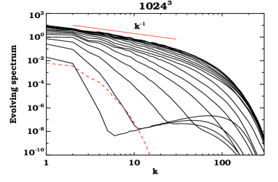
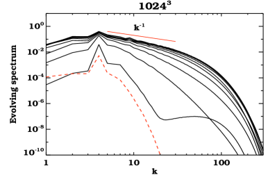
Figure 2: The left panel shows the growing scalar spectrum as solid lines for run A from times $t=5-80$ every $5$ time units. Time increases from the bottom to the top curve and the topmost curve shows the steady state scalar spectrum. The steady velocity spectrum is shown as a dashed line. Within $t=20$ the rms velocity rises to $u_{rms}\sim 0.15$ and varies between $0.13-0.17$, of the sound speed. The right panel shows the corresponding spectra for run B. The scalar spectra are shown from $t=5-45$ every $5$ time units. Within $t=10$ the rms velocity settles to $u_{rms}\sim 0.11$ in units of the sound speed.

In Fig. 2, we show as solid lines, the evolution of the passive scalar power spectrum, $E_{\theta}$, in equal time intervals. The steady state velocity spectrum is also shown, by a dashed line. The left panel is for run A with $k_{f}=1.5$ and the right panel is for run B with $k_{f}=4$. The rms velocities in units of the sound speed are $u_{rms}\sim 0.15$ and $u_{rms}\sim 0.11$ in runs A and B respectively, such that the incompressibility condition is well satisfied, and $\rho$ is nearly constant. The viscosity has been set high enough that the flow is almost single scale, and the diffusivity low enough that the Peclet and Schmidt numbers are high. We have $Sc=400$, $R_{\kappa}\sim 4000$ and $Sc=100$, $R_{\kappa}=250$ for the runs A and B respectively. Thus one would expect indeed to obtain a significant viscous-convective range of wavenumbers. the simulations are then suited to test if one obtains the Batchelor $E_{\theta}\propto 1/k$ spectrum, in steady state. The simulation were run for a sufficiently long time to obtain steady state in evolution of the passive scalar, as can be seen from the overlap of the spectrum at final times. As can be seen from both the panels in Fig. 2, $E_{\theta}$ reaches a steady state and exhibits a scale dependence of $k^{-1}$ to a reasonable degree in the viscous-convective range larger than $k_{f}$. While Kraichnan’s idealistic model of delta-correlation predicted $k^{-1}$ spectrum, the solution to our extended Kraichnan equation showed that to the leading order, finite time correlation does not change this scale dependence. This is also predicted by the Lagrangian analysis (Falkovich et al., 2001). We find that our DNS which explores Schmidt numbers up to $400$ bears this out. We note that earlier DNS, with higher Re than obtained here, but with $Sc$ up to 64, have also found evidence for the Batchelor spectrum in the viscous-convective range (see Donzis et al. (2010); Gotoh & Yeung (2013) and references therein). During the course of this work, we also came across some recent very high resolution hybrid simulations of passive scalar mixing with $Sc\sim 200-1000$ comparable to ours, which also reports reasonable agreement with the steady state Batchelor spectrum (Gotoh et al., 2014). There have been interesting predictions for the behaviour of higher order correlators in the steady state and the influence of the diffusive scale even on larger scales (Balkovsky et al., 1995; Chertkov et al., 2007). It would be of interest to check for such effects in future work.

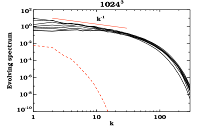
Figure 3: The left panel shows the decaying scalar spectrum (solid lines) from $t=80-140$ in steps of $10$ time units for run A. The corresponding decay phase for run B is shown on the right panel, from $t=40-105$ in steps of $5$ time units. Time now increases from the top to the bottom curves. The topmost curve again shows the steady state spectrum from which the decay began, once the scalar forcing is turned off. The dashed lines again show the steady state velocity spectrum.

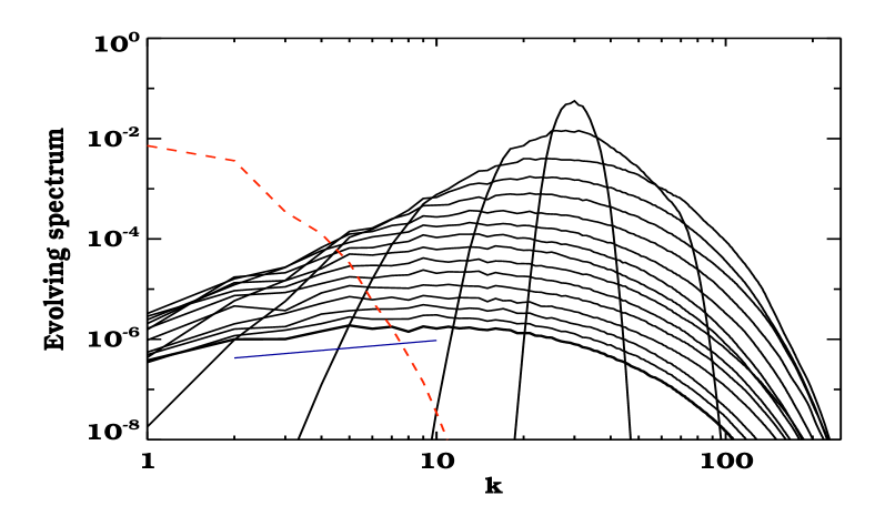
Figure 4: The figure shows the decaying scalar spectrum (solid lines) when one starts from initial power peaked at $k_{0}=30$. The topmost curve shows the spectrum at $t=5$ or after about 1 eddy turn over time after the the decay began, with the scalar forcing is turned off. Subsequent curves, from top to bottom, are shown for times $t=5,10,20,.......,150$. The blue solid straight line shown at the bottom is $E(k)\propto k^{1/2}$. The dashed line again shows the (almost) steady state velocity spectrum. Within $t=5$ the rms velocity rises to $u_{rms}\sim 0.1$ and varies between $0.11-0.15$, of the sound speed.

5.2 DNS of passive scalar decay

We next examine the decay of the passive scalar through our DNS. We carry out two types of DNS to explore this phase. In the first case, to obtain such a decay, we turn off the imposed constant gradient in the passive scalar equation. The passive scalar spectrum then decays from its initial steady state, as is shown in Fig. 3. We find that the spectrum flattens as it decays, but never becomes close to the $k^{1/2}$ form predicted by the analytic argument. This can be seen to obtain in both Run A (left panel of Fig. 3) and in Run B (right panel). It could be that the box scale mode decays slower due to turbulent diffusion, at a rate $\sim k_{box}^{2}\kappa_{t}$, with $k_{box}=1$ in our DNS, compared to the small scale modes. Our analytical considerations predict that they decay at the rate $\sim q^{2}\kappa_{t}$, with $q\sim k_{f}$. Some evidence for such an idea is seen in Run B, where there is a clear separation of scales. Then the box scale modes could act as a source for the small scale fluctuations, leading to a spectrum flatter than $k^{1/2}$ but not as steep as $k^{-1}$. A similar idea has been explored in Schekochihin et al. (2004).

In view of the above, we carry out a second type of DNS where we make sure that there is no large-scale power in the scalar fluctuations at the initial time. In particular, we start the decay with scalar power peaked initially at some wavenumber $k_{0}\gg k_{f}$ and let it decay due to the random motions driven at the forcing wavenumber $k_{f}$. This is analogous to the case of the solved example, presented in Section  4.3.1 and appendix B. In Fig. 4, we show the results from such a high resolution run ($N=1024$, Run C), where the initial scalar spectrum is a delta function at $k_{0}=30$ and $k_{f}=1.5$. The subsequent decay of the scalar spectrum is shown as a sequence of solid curves in Fig. 4. The curves from top to bottom correspond to times $t=5,10,20,30,......,150$. The blue straight line is the 1-D scalar spectrum which is predicted at the low k end in the Batchelor regime, $E_{\theta}(k)\propto k^{1/2}$.

The decay now is more in line with expectations. By $t=5$, which is roughly one eddy turn over time, the spectrum has spread to have almost a Gaussian shape, although still peaked at around $k\sim k_{0}=30$. As the decay proceeds, the scalar power spreads, with its half width increasing in time. The slope at low $k$ is always positive now, but steeper than the $k^{1/2}$ form because of the influence of the expected rise of power towards $k_{0}$, the Gaussian part in Eq. (88). Power reaches the diffusive cut-off scale $k_{d}\sim 90$, by $t=20$, after which it cannot spread further to larger $k$, but continues to spread to smaller and smaller $k<k_{0}$. The peak of the spectrum thus shifts to smaller and smaller $k<k_{0}$ as the scalar power decays. The power at $k=1$ increases till about $t=60$, stays roughly constant and later after $t=90$ starts decaying. In fact after about $t=90$ till $t=140$, the spectra shift down almost like an eigenfunction, preserving their shape. Towards the end of the simulation, the low-$k$ slope of the scalar spectrum approaches the $k^{1/2}$ form (see Figure 4), with the peak of the spectrum at $k\sim 10$. Eventually, the box scale modes are expected to decay slower than the modes with $k>k_{f}$ and one could see a further flattening of the spectrum. All in all this DNS shows that the theory of scalar decay developed for the Kraichnan model and its generalization, in Section 4.3, is borne out to a reasonable extent.

6 Discussion and Conclusions

The mixing and decay of a passive scalar by random or turbulent flows which are spatially smooth on scales where the scalar still has structure, is important in several contexts in nature and industry. This regime obtains when the Schmidt number (the ratio of viscosity to scalar diffusivity) is large; for example $Sc\sim 10$ for flow of heat in water and of order $1000$ for several organic liquids (Gotoh & Yeung, 2013). The passive scalars then develops finer scale structure than the velocity itself. Batchelor (1959) developed a theory for the steady state spectrum of fluctuations generated in such mixing, and argued that $E_{\theta}(k)\propto 1/k$, a spectral form known as the Batchelor spectrum. This spectrum was shown to obtain as a steady state solution to the evolution equation for $E_{\theta}$ by Kraichnan (1968).

Kraichnan’s theory of passive scalar mixing and decay in such flows assumed delta-correlation in time. However, the correlation time is expected to be finite in realistic random flows. We have extended here the study of passive scalar mixing and decay to finite correlation times, by using a model of random single scale velocity field that renews itself after every time interval $\tau$. In particular, we present a detailed derivation of the evolution equation for the power spectrum and the two-point correlation of the passive scalar in renewing flows. For this purpose, we used an ensemble average over the random flow, following one renewing step at a time. We arrived at the generalised Kraichnan equation which includes leading next order contributions in $\tau$ when compared to the original Kraichnan equation itself. As we explicitly point out above, this equation involves fourth order velocity correlators, which for our flow, are not just products of the two-point velocity correlator. We note that our differential equation approach to finite $\tau$ effects is essentially new, and complementary to the ’integral’ Lagrangian approaches to the same problem (Falkovich et al., 2001), reviewed in Appendix-A.

The generalised Kraichnan equation in Fourier space derived here, applicable to the viscous-convective range, contains new contributions which involve higher order (third and fourth) derivatives of the passive scalar power spectrum $\hat{M}(k,t)$. However, these higher order terms appear only perturbatively in $\bar{\tau}=\kappa_{t}q^{2}\tau$. As in BS15, one can then use the Landau-Lifshitz approach, earlier used to handle the radiation reaction force, to rewrite these terms, to involve those with at most second derivatives of $\hat{M}(k,t)$.

The resulting evolution equation is analyzed, in terms of eigenmodes, using both a scaling solution valid in the viscous-convective range, and also a more exact solution including diffusive effects. Two cases are considered. First, the steady state situation which one would obtain if there was also a source of passive scalar fluctuations at low wave numbers, that maintains the scalar fluctuations against decay. Second, the turbulent decay case, where there is no such source.

An important consequence of the generalized Kraichnan equation is that, its steady state solution for the passive scalar spectrum in the viscous-convective regime, still preserves the Batchelor form $E_{\theta}(k)\propto 1/k$, for a finite $\tau$ to leading order in $\tau$. In fact the generalized Kraichnan equation (48) for the steady state scalar spectrum $\tilde{M}(k)$, which takes into account the effect of a finite $\tau$, is exactly the same as that derived under the delta-correlation in time approximation by Kraichnan (1968). To some extent, this result is expected from both the work of B59 and the several subsequent works using a Lagrangian analysis of the general finite $\tau$ case (cf. Falkovich et al. (2001) and references therein; see also Appendix A). However, our approach in terms of the generalized Kraichnan equation is different and complementary to the earlier work. It also allows for a non-Gaussian velocity field.

A new result of our work, concerns the scalar spectrum for the decaying case, when there is no source. This is analyzed in terms of eigenmodes and the corresponding Green’s function solution to the initial value problem.We have shown here that at late times, the qualitative form of this spectrum is also independent of $\tau$ to leading order in $\tau$, and in the Batchelor regime, has a dominant form $E_{\theta}\propto k^{1/2}$. This result, is found by Vergeles (2006) in the Lagrangian approach for the Kraichnan problem with $\tau=0$. However, for a finite $\tau$, it is not apparent in Lagrangian approaches, as it requires an explicit evaluation of the probability function $P(X)$ at finite $\tau$, which is non trivial. It illustrates the usefulness of our complementary, differential equation approach to the finite $\tau$ passive scalar problem. We also showed that the scalar fluctuations seeded at some initial $k_{0}$ spread in time and in addition, have an overall exponential decay at the turbulent diffusion rate. An exponential decay of the scalar variance in the Batchelor limit of the Kraichnan equation has been pointed out earlier (Balkovsky & Fouxon, 1999; Son, 1999). The decay rates are however reduced for a finite $\tau$ compared to the delta-correlated flow. More work incorporating a large-scale cut-off in velocity correlations would be important to understand scalar decay, not only in the Kraichnan limit, but also its extensions to the finite $\tau$ case.

Further, to test the analytics we have carried out high resolution ($1024^{3}$) DNS of passive scalar mixing at high Schmidt number up to 400, and Peclet numbers 10 times larger. Such high Schmidt and Peclet numbers are comparable to the highest values realized so far, for examining the validity of the Batchelor steady state spectrum. Our DNS results lend reasonable support to the Batchelor $E_{\theta}\propto 1/k$ scaling when a steady state is maintained by a low wavenumber source.

Moreover, we have also used high resolution DNS to explore the turbulent decay case, when there are no sources of scalar fluctuations. We have examined decay from two types of initial conditions. In the first case, we start the decay from the steady state spectrum by turning of the scalar source. In this case, the passive scalar spectrum during decay, flattens from the Batchelor $E_{\theta}(k)\propto(1/k)$ form. However it does not become as steep as the $k^{1/2}$ spectrum predicted by both the Kraichnan model and its finite $\tau$ generalization presented here. This result which is new could arise due to the fact that lower wavenumber, box scale, scalar fluctuations decay at a smaller rate, $k_{box}^{2}\kappa_{t}$, compared to the small scale ones, which decay at the rate $\sim k_{f}^{2}\kappa_{t}$. They can then continue to source the small scale fluctuations, and lead to a shallower spectrum.

We have also carried out DNS of decay where the scalar spectrum is initially peaked at some wavenumber $k_{0}\gg k_{f}$, such that the box scale modes $k<k_{f}$ are grossly sub dominant. The decay behaviour from the DNS is now more in line with expectations from the analytics. The scalar power spreads as it decays, with the spectrum having a positive slope at low $k$ at all times. At late times, when the range over which the scalar spectrum extent becomes large enough, one sees the emergence of $E_{\theta}\propto k^{1/2}$ behaviour in the Batchelor regime, at $k>k_{f}$. At even later times, one would expect the box scale power (which decays slower) to become important, and a further flattening of the spectrum as described above.

We used the renewing flow to derive the generalized Kraichnan equation; however the resulting evolution equation can be written in terms of velocity correlators $T_{ij}$ and $T_{ijkl}$ in a general form. It also matches exactly with the corresponding real and Fourier space Kraichnan equations derived assuming delta-correlated flow in the appropriate limit of $\tau\to 0$. Thus they could have more general validity than the context of renewing flows, in which they are derived. An analysis of this finite $\tau$ equation incorporating both scale dependent velocity correlators and correlation times (cf. Chertkov et al. (1996); Eyink & Xin (2000); Adzhemyan et al. (2002); Chaves et al. (2003)) would be useful. It would also be of interest to try and extend our results to the non-perturbative regime, through both the current approach and a Lagrangian analysis. In addition, it will be fruitful to include the effects of shear and rotation, which are often present in realistic turbulent flows.

Appendix A Lagrangian analysis of Passive scalar mixing

We review here a Lagrangian analysis for passive scalar mixing following to some extent Falkovich et al. (2001). This will also clarify the conditions under which one can derive from such an analysis, the Batchelor spectrum or the scalar spectrum when its fluctuations decay, for a general renovation time $\tau$.

Adding a source term to Eq. (1) for the evolution of the passive scalar field $\theta(\mbox{\boldmath$x$},t)$ gives,

$$\frac{\partial\theta}{\partial t}+\mbox{\boldmath$u$}\cdot{\bf\nabla}\theta=\frac{D\theta}{Dt}=f_{\theta}(\mbox{\boldmath$x$},t)+\kappa\nabla^{2}\theta,$$ (72)

Suppose we consider scales where diffusion can be neglected. Then the formal solution to Eq. (72) is

$$\theta(\mbox{\boldmath$x$},t)=\theta_{0}(\mbox{$\mbox{\boldmath$x$}_{0}$},t_{0})+\int_{t_{0}}^{t}f_{\theta}(\mbox{\boldmath$x$}(t^{\prime}),t^{\prime})dt^{\prime}$$ (73)

where $\theta_{0}$ is the initial scalar field and the integration of the source is along the Lagrangian trajectory of a particle frozen to the flow. Further $\mbox{$\mbox{\boldmath$x$}_{0}$}=\mbox{\boldmath$x$}(t_{0})$ in $\theta_{0}$ is related to $\mbox{\boldmath$x$}(t)$ in $\theta$ by integrating back in time along the Lagrangian trajectory.

A.1 The steady state Batchelor spectrum

To begin with, let us assume that the initial scalar field fluctuations are either small or have decayed, and focus on those sustained by the source term. The two-point spatial correlation function of the passive scalar, as defined by Eq. (6), then evolves as,

$$M(r,t)=\left\langle\int_{t_{0}}^{t}dt^{\prime}\int_{t_{0}}^{t}dsf_{\theta}(\mbox{\boldmath$x$}(t^{\prime}),t^{\prime})f_{\theta}(\mbox{\boldmath$y$}(s),s)\right\rangle,$$ (74)

where the source is assumed to be uncorrelated with the initial scalar field $\theta_{0}$ and $r=|\mbox{\boldmath$x$}-\mbox{\boldmath$y$}|$ as before. The averages over $f_{\theta}$ involves both average over the source statistics and that over the random Lagrangian trajectories $\mbox{\boldmath$x$}(t^{\prime})$ and $\mbox{\boldmath$y$}(t^{\prime})$. It is generally assumed (Falkovich et al., 2001), that the source is statistically homogeneous, isotropic, Gaussian, of zero mean and variance which is delta-correlated in time, i.e

$$\langle f_{\theta}(\mbox{\boldmath$x$},t^{\prime})f_{\theta}(\mbox{\boldmath$y$},s)\rangle=\Psi\left(\frac{r}{L}\right)\delta(t^{\prime}-s).$$ (75)

Here $L$ is some fiducial length scale over which $\Psi$ varies. Using Eq. (75) in Eq. (74), we have

$$M(r,t)=\langle\int_{t_{0}}^{t}dt^{\prime}\ \Psi\left(\frac{r(t^{\prime})}{L}\right)\rangle=\int\int_{t_{0}}^{t}dt^{\prime}\ \Psi\left(\frac{r^{\prime}}{L}\right)P(r^{\prime},r;t,t^{\prime})dr^{\prime}.$$ (76)

The averaging in the first part of the equation is over the random Lagrangian trajectories of a pair of particles frozen to the flow, whose separation is $r(t^{\prime})$ at time $t^{\prime}$. In the latter part of the equation this has been written in terms of the two-particle pair probability $P(r^{\prime},r;t^{\prime},t)dr^{\prime}$, that for a given pair separation, $r=r(t)$ at time $t$, the pair separation is $r^{\prime}=r(t^{\prime})$ at an earlier time $t^{\prime}$. For finding this probability we have to follow a pair of particles, backward in time from $t$ to $t^{\prime}$. However, some general results can be obtained even without finding the exact form of $P$.

Suppose the flow has a correlation time $\tau$ much smaller than the time $T=t-t_{0}$. Then the Lagrangian trajectory will be comprised of many uncorrelated steps. For our renewing flow in particular, the frozen in pair of particle will take $N=T/\tau$ random steps. For a smooth flow, like the one we consider, in the Batchelor regime, with $1/k_{\kappa}\ll r\ll 1/q$, the mean pair separation is expected to increase exponentially fast, with $r_{0}/r=\exp(\bar{\lambda}T)$. Here $\bar{\lambda}>0$ (see below) and $-\bar{\lambda}$ is the Lyapunov exponent for the contracting direction, when going forward in time (cf. Eq. (138) of Falkovich et al. (2001)), and is negative for an incompressible flow. We will calculate $\bar{\lambda}$ explicitly below in the Kraichnan limit. For sufficiently large $N\gg 1$, the peak of the probability distribution $P$ then shifts to $r^{\prime}=r\exp(\bar{\lambda}T^{\prime})$ as $T^{\prime}=t-t^{\prime}$ increases backward in time. We can then approximate the integral in Eq. (76) as follows.

We note that significant contribution to the integral over $r^{\prime}$ will obtain only for $r^{\prime}<L$, corresponding to a time $T^{\prime}<T_{*}=\bar{\lambda}^{-1}\ln(L/r)$. Let us approximate the value of $\Psi(r)$ in this range by its value at the origin, $\Psi_{0}$. Then

$$M(r,t)\approx\Psi_{0}\int_{0}^{T_{*}}dT^{\prime}=\Psi_{0}T_{*}=\frac{\Psi_{0}}{\bar{\lambda}}\ln\left(\frac{L}{r}\right).$$ (77)

The logarithmic form of the two-point spatial correlator in Eq. (77) is equivalent to the $E_{\theta}(k)\propto 1/k$ form of the Batchelor spectrum. Thus the Batchelor spectrum arises in a fairly general manner independent of the value of the renewal time $\tau$. We emphasize that the above derivation involves some simplifying assumptions: (1) The source is delta-correlated in time; one could replace this with a sufficiently short correlation time compared to $T$, such that $N\gg 1$. (2) The spatial variation of $\Psi(r)$ can be neglected in the Batchelor regime. This is equivalent to assuming that in spectral space the source contributes only at low $k$ outside the viscous-convective range of $k$. (3) The width of the probability distribution $P$ is narrow enough that only the location of its peak is important in determining $T_{*}$.

In this context, we note that the derivation of the Batchelor spectrum given in the main text, using the extended Kraichnan differential equation Eq. (44), does involve making assumption (2) above, but not (1) and (3) in an explicit manner. Thus it offers a complementary approach to the problem, albeit an approach which can at present only recover the Batchelor spectrum for a finite $\tau$ in the perturbative limit.

A.2 The Lyapunov exponent for the renewing flow

Let us now turn to an explicit derivation of $\bar{\lambda}$ for renewing flows, in the case of a short renewal time $\tau$ and in the limit of a linearly varying velocity field. We expand Eq. (2) about $\mbox{\boldmath$x$}=0$ keeping only up to terms linear in $x$. Thus the velocity field is taken to be

$$\mbox{\boldmath$u$}=\mbox{\boldmath$a$}(\mbox{\boldmath$q$}\cdot\mbox{\boldmath$x$})\cos\psi+\mbox{\boldmath$a$}\sin\psi$$ (78)

in each renewing flow step, with $a$, $q$ and $\psi$ having the same statistical properties as before.

Suppose the time interval $T=t-t_{0}=N\tau$, corresponding to $N$ intervals of the renewing flow. Consider a pair of points frozen to the flow which at time $t$ have a separation $r=r(t)$ and at time $t_{0}$ a separation $r_{0}=r(t_{0})$. Here $r(t)=|\mbox{\boldmath$r$}|$ where as before $\mbox{\boldmath$r$}(t)=(\mbox{\boldmath$x$}(t)-\mbox{\boldmath$y$}(t))$. Let the pair separation at an intermediate time $t_{n}=t_{0}+n\tau$ be $r_{n}=r(t_{n})$. Thus $n=0$ corresponds to the time $t_{0}$ and $n=N$ to the time $t$. Then

$$\frac{r_{0}}{r}=\frac{r_{0}}{r_{1}}\frac{r_{1}}{r_{2}}.....\frac{r_{N-1}}{r}$$ (79)

Thus the ratio of the initial to final pair separation is a product of $N$ random variables. To work out its statistical properties, it is useful to take its logarithm and consider this as the sum of N random variables,

$$X=\ln\left(\frac{r_{0}}{r}\right)=\sum_{n=1}^{N}\ln\left(\frac{r_{n-1}}{r_{n}}\right)=\sum_{n=1}^{N}x_{n}$$ (80)

where $x_{n}=(r_{n-1}/r_{n})$. Note that the mean of each $x_{n}$, defined as $\langle x_{n}\rangle=\mu$, is identical as each renewing flow step has the same statistical properties. Then the mean of the random variable $X$ is $\langle X\rangle=N\mu$. This can be used to define the Lyapunov exponent

$$\bar{\lambda}=\lim_{t\to\infty}\frac{1}{t}\left\langle\ln\left(\frac{r_{0}}{r}\right)\right\rangle=\lim_{N\to\infty}\frac{\langle X\rangle}{N\tau}=\frac{\mu}{\tau}.$$ (81)

(For our renewing flow, as we show below, one gets the same Lyapunov exponent $\bar{\lambda}$ if we calculate the exponential increase in pair separation going forward in time). To calculate $\mu$, we need to relate the pair separation at time $t_{n}$ to that at time $t_{n-1}$. Now integrating $d\mbox{\boldmath$x$}/dt=\mbox{\boldmath$u$}$ backward in time for a time $\tau$, noting again that $\mbox{\boldmath$q$}\cdot\mbox{\boldmath$x$}$ is constant for an incompressible flow, the evolution of pair separation is given by,

$$\mbox{\boldmath$r$}_{n-1}=\mbox{\boldmath$r$}(t_{n-1})=\mbox{\boldmath$r$}_{n}-\tau\mbox{\boldmath$a$}(\mbox{\boldmath$q$}\cdot\mbox{\boldmath$r$}_{n})\cos\psi$$ (82)

for each step $\tau$ back in time. Taking the amplitude of the vectors on both sides of Eq. (82), gives

$$x_{n}=\frac{1}{2}\ln\left[1-2\tau\cos\psi(\mbox{\boldmath$a$}\cdot\hat{\mbox{\boldmath$r$}}_{n})(\mbox{\boldmath$q$}\cdot\hat{\mbox{\boldmath$r$}}_{n})+\tau^{2}\cos^{2}\psi(\mbox{\boldmath$q$}\cdot\hat{\mbox{\boldmath$r$}}_{n})^{2}\right]=\frac{1}{2}\ln[1+\tau\alpha+\tau^{2}\beta],$$ (83)

where we have defined $\alpha=-2\cos\psi(\mbox{\boldmath$a$}\cdot\hat{\mbox{\boldmath$r$}}_{n})(\mbox{\boldmath$q$}\cdot\hat{\mbox{\boldmath$r$}}_{n})$, $\beta=\cos^{2}\psi(\mbox{\boldmath$q$}\cdot\hat{\mbox{\boldmath$r$}}_{n})^{2}$ and $\hat{\mbox{\boldmath$r$}}_{n}$ is the unit vector $\mbox{\boldmath$r$}_{n}/r_{n}$.

Note that $\mu=\langle x_{n}\rangle$ is difficult to calculate analytically for a general $\tau$ because all the random variables over which averages have to be taken are inside a logarithm. This is the reason it is difficult to calculate $P$ exactly for a general $\tau$ and also hence the properties of the decaying scalar spectrum exactly (see below). Recall that estimating the form of the steady state spectrum did not require explicit calculation of $\bar{\lambda}$ or $\mu$. However, $\mu$ and various other statistical moments of $x_{n}$ can be calculated perturbatively for small $\tau$ by expanding the logarithm in Eq. (83) as a power series in $\tau$ about $\tau=0$.

It is also interesting to point out that powers of $\tau$ are always accompanied by the same powers of $\cos\psi$. As odd powers of $\cos\psi$ average to zero, all moments of $x_{n}$ depend only on even powers of $\tau$. Therefore the Lyapunov exponent defined by calculating the increase of pair separation going forward in time, is same as that defined going back in time. Together with the incompressibility condition, this also implies that the three Lyapunov exponents for the renewing flow are given by $(\bar{\lambda},0,-\bar{\lambda})$.

We calculate here just the lowest order contribution to $\mu$ which can be obtained by expanding the logarithm in Eq. (83) to up to $\tau^{2}$ terms. This gives,

$$\mu=\frac{1}{2}\tau^{2}\left\langle\left(\beta-\frac{\alpha^{2}}{2}\right)\right\rangle=\frac{A^{2}\tau^{2}q^{2}}{30}=\frac{3}{5}\kappa_{t}q^{2}\tau$$ (84)

Thus the Lyapunov exponent $\bar{\lambda}=\mu/\tau=(3/5)\kappa_{t}q^{2}$ is of the order the turbulent diffusion rate.

A.3 The passive scalar correlations during decay

We briefly comment on the case when the source is absent. We saw in the main text that the passive scalar fluctuations decay in this case, with a characteristic spectrum $E_{\theta}\propto k^{1/2}$ in the Kraichnan limit. We also showed that interestingly, the spectral form $E_{\theta}\propto k^{1/2}$ is preserved even at finite $\tau$ to leading order in $\tau$, although the decay rate decreases for a finite $\tau$. One may wonder if such results can and have been obtained in a Lagrangian analysis.

In the absence of a source, the two-point spatial correlation evolves as,

$$M(r,t)=\left\langle\theta(\mbox{$\mbox{\boldmath$x$}_{0}$},t_{0})\theta(\mbox{$\mbox{\boldmath$y$}_{0}$},t_{0})\right\rangle=\int dr_{0}\ P(r_{0},r;t_{0},t)\ M(r_{0},t_{0}).$$ (85)

Here we have assumed that the passive scalar at any time is statistically isotropic and homogeneous and again averaged over the random pairs of Lagrangian trajectories which reach a separation $r$ at time $t$ starting from a separation $r_{0}$ at time $t_{0}$. This is explicitly incorporated by weighting $M(r_{0},t_{0})$ by the pair probability density $P(r_{0},r;t_{0},t)$ and integrating over $r_{0}$.

Note that Eq. (85) gives an integral equation for the spatial correlation $M(r,t)$. Its solution depends on knowing the explicit form of the probability $P$. This is unlike the steady state case, when one only needed to know that particle trajectories separate exponentially fast in a smooth random flow. In order to calculate $P$ for a general $\tau$, one would need to know for example its moments and this in turn involves all the moments of $x_{n}$. As we noted above, calculating the moments of $x_{n}$ involves carrying out various statistical averages over $a$, $q$ and $\psi$, which are inside a logarithm. This cannot be done analytically for a general $\tau$, and hence the difficulty with going beyond the Kraichnan limit for the decaying case correlators. Indeed due to the logarithmic form of $x_{n}$, one expects its statistics and hence $P(x)$ to be strongly non-Gaussian as well.

The probability $P(x)$ however becomes Gaussian in $\ln(r_{0}/r)$ (or log-normal in $r_{0}$) in the Kraichnan limit (cf. Falkovich et al. (2001) and references therein). The mean value of $P(X)$ is given by $N\mu$ and dispersion by $N\sigma^{2}$, where $\sigma^{2}$ is the variance of $x_{n}$ calculated also perturbatively. In this case, the integral equation can be analysed to show that $M(r,t)\propto r^{-3/2}$, which corresponds to the $E_{\theta}\propto k^{1/2}$ spectrum (cf. Vergeles (2006)). However, the result shown in the main text, that the scalar spectrum in this case, is also left invariant for a finite $\tau$ to leading order, does not appear to have been shown using a Lagrangian analysis. This again illustrates the usefulness of the complementary, differential equation approach to the passive scalar problem, in terms of the extended Kraichnan equation, discussed in the main text. We plan to return to a more detailed discussion of the Lagrangian analysis for the decaying case in future work, also including the effects of scalar diffusion neglected above.

Appendix B A solved example of scalar spectral evolution

To get some further insight into the evolution of the scalar spectrum implied by Eq. (66), we consider an analytically solvable example. As in the main text, assume $\hat{M}(k,0)=\delta(k-k_{0})/(4\pi k^{2})$. We are particularly interested also in the small $k/k_{d}\ll 1$ behaviour of the spectrum, (as we expect the spectrum to decay at large $k/k_{d}\gg 1$; see below). In this limit, using Eq. (57), and carrying out trivially the $k^{\prime}$ integral of Eq. (66), the scalar spectral evolution is given by

$$\hat{M}(k,t) = \frac{2}{\pi}k^{-3/2}k_{0}^{-3/2}e^{-\bar{\gamma}\bar{t}}\int_{0}^{\infty}d\mu\ \exp\left(-\frac{4}{9}\mu^{2}\bar{\gamma}\bar{t}\ \frac{(1-9\bar{\gamma}\bar{\tau}/14)}{(1+2\mu^{2}\bar{\gamma}\bar{\tau}/7)}\right)$$ (86)

$$\times \sin\left(\mu\ln(k/2k_{d})+c_{\mu}\right)\sin\left(\mu\ln(k_{0}/2k_{d})+c_{\mu}\right).$$

As discussed above, due to the damping factor $\exp(-\gamma(\mu))\bar{t})$, which monotonically increases with $\mu$, the $\mu$ integral will be dominated by the contribution from the vicinity of small $\mu$. As time increases this range of $\mu$ decreases and will be confined to $\mu<\mu_{0}\approx 1/\sqrt{\bar{\gamma}\bar{t}}$.

We can then approximate $2\mu^{2}\bar{\gamma}\bar{\tau}/7\sim\bar{\tau}/\bar{t}\ll 1$, and $(1+2\mu^{2}\bar{\gamma}\bar{\tau}/7)\approx 1$. Moreover in Eq. (86), the product $2\sin(\mu\ln(k/2k_{d})+c_{\mu})\sin(\mu\ln(k_{0}/2k_{d})+c_{\mu})=\cos[\mu\ln(k/k_{0})]-\cos[\mu\ln(kk_{0}/4k_{d}^{2})+2c_{\mu}]$. Then Eq. (86) becomes,

$$\hat{M}(k,\bar{t})=\frac{1}{\pi}k^{-3/2}k_{0}^{-3/2}e^{-\bar{\gamma}\bar{t}}\int_{0}^{\infty}d\mu\ e^{-\beta\mu^{2}\bar{t}}\left[\cos\left(\mu\ln\left(\frac{k}{k_{0}}\right)\right)-\cos\left(\mu\ln\left(\frac{kk_{0}}{4k_{d}^{2}}\right)+2c_{\mu}\right)\right],$$ (87)

where we have defined $\beta=4\bar{\gamma}(1-9\bar{\gamma}\bar{\tau}/14)/9$. The integral over $\mu$ involving the first cosine term in Eq. (87) can be done exactly, while the presence of $c_{\mu}$ prevents one from an exact evaluation of the second cosine term. However, as $(kk_{0}/k_{d}^{2})/(k/k_{0})=k_{0}^{2}/k_{d}^{2}\ll 1$ and also $(kk_{0}/k_{d}^{2})\ll 1$, we will have for any $k$, $|\ln(kk_{0}/4k_{d}^{2})|\gg|\ln(k/k_{0})|$. The phase of the cosine in the second integral will then vary much more rapidly compared than the phase of the cosine in the first integral, as $\mu$ varies. Thus the second integral will suffer from much larger cancellations and hence is sub-dominant compared to the first. Then evaluating the first integral in Eq. (87), we get for the one-dimensional scalar spectrum

$$E_{\theta}(k,\bar{t})=4\pi k^{2}\tilde{M}(k,\bar{t})=e^{-\bar{\gamma}\bar{t}}\left(\frac{k}{k_{0}}\right)^{1/2}\frac{2}{k_{0}}\sqrt{\frac{\pi}{\beta\bar{t}}}\exp\left(-\frac{[\ln(k/k_{0})]^{2}}{4\beta\bar{t}}\right)$$ (88)

(We note in passing that the second integral can also be evaluated exactly at late times, as then the integral is dominated by $\mu<1/\sqrt{\bar{\gamma}\bar{t}}\ll 1$, and we can take $c_{\mu}\approx\bar{c}\mu$. Then the second integral gives a contribution with $\ln(k/k_{0})$ in Eq. (88) replaced by $\ln(kk_{0}/4k_{d}^{2})+2\bar{c}$. As discussed above, $(\ln(kk_{0}/4k_{d}^{2}))^{2}\gg(\ln(k/k_{0}))^{2}$, and thus the second term can be seen to be explicitly sub dominant compared to the first integral and hence its neglect above justified.)

We see from Eq. (88) that the evolution of the scalar spectrum seeded at $k_{0}$ is as expected earlier on qualitative grounds. It evolves in time with $E_{\theta}$ taking the form of a Gaussian in $\ln(k/k_{0})$, with the Gaussian width increasing as $\sqrt{\beta\bar{t}}$, and multiplied by an overall factor $\propto(k/k_{0})^{1/2}$. When the width becomes large enough, we expect the $k^{1/2}$ form of the spectrum to dominate near the maximum of the Gaussian. Apart from the spreading of the scalar power, there is also overall exponential decay at the rate $\bar{\gamma}$ (or of order the turbulent diffusion rate in dimensional units).

Note also that $\bar{\tau}$ appears only in $\bar{\gamma}$ and $\beta$, thus the qualitative form of the spectrum is independent of $\tau$. This is an important result that a finite $\tau$ does not qualitatively change the shape of the scalar spectrum during decay. Further, both $\bar{\gamma}$ and $\beta$ are smaller for $\tau\neq 0$ compared to the Kraichnan case of $\tau\to 0$. Thus the decay of scalar fluctuations is slowed down for a non zero $\tau$. The above analysis is valid provided $k/k_{d}\ll 1$. Once the spectrum has spread to diffusive scales with $k/k_{d}>1$, or for more general initial conditions, an analytic evaluation of the integrals in Eq. (66) is no longer possible, and we have to treat the problem numerically, as done in the main text.

References

- Abramowitz & Stegun (1972) Abramowitz, M. & Stegun, I. A. 1972 Handbook of Mathematical Functions.
- Adzhemyan et al. (2002) Adzhemyan, L. T., Antonov, N. V. & Honkonen, J. 2002 Anomalous scaling of a passive scalar advected by the turbulent velocity field with finite correlation time: Two-loop approximation. PRE 66 (3), 036313, arXiv: nlin/0204044.
- Balkovsky et al. (1995) Balkovsky, E., Chertkov, M., Kolokolov, I. & Lebedev, V. 1995 Fourth-order correlation function of a randomly advected passive scalar. Journal of Experimental and Theoretical Physics Letters 61, 1049.
- Balkovsky & Fouxon (1999) Balkovsky, E. & Fouxon, A. 1999 Universal long-time properties of Lagrangian statistics in the Batchelor regime and their application to the passive scalar problem. PRE 60, 4164–4174.
- Batchelor (1959) Batchelor, G. K. 1959 Small-scale variation of convected quantities like temperature in turbulent fluid. Part 1. General discussion and the case of small conductivity. Journal of Fluid Mechanics 5, 113–133.
- Bhat & Subramanian (2014) Bhat, P. & Subramanian, K. 2014 Fluctuation Dynamo at Finite Correlation Times and the Kazantsev Spectrum. ApJ 791, L34, arXiv: 1406.4250.
- Bhat & Subramanian (2015) Bhat, P. & Subramanian, K. 2015 Fluctuation dynamos at finite correlation times using renewing flows. Journal of Plasma Physics 81.
- Brandenburg (2003) Brandenburg, A. 2003 Computational aspects of astrophysical MHD and turbulence. In Advances in Nonlinear Dynamos (ed. A. Ferriz-Mas & M. Núñez), pp. 269–344. Taylor & Francis, London and New York.
- Brandenburg & Dobler (2002) Brandenburg, A. & Dobler, W. 2002 Hydromagnetic turbulence in computer simulations. Computer Physics Communications 147, 471–475, arXiv: arXiv:astro-ph/0111569.
- Chaves et al. (2001) Chaves, M., Eyink, G., Frisch, U. & Vergassola, M. 2001 Universal Decay of Scalar Turbulence. Physical Review Letters 86, 2305–2308, arXiv: nlin/0010011.
- Chaves et al. (2003) Chaves, Marta, Gawedzki, Krzysztof, Horvai, Peter, Kupiainen, Antti & Vergassola, Massimo 2003 Lagrangian dispersion in gaussian self-similar velocity ensembles. Journal of Statistical Physics 113 (5), 643–692.
- Chertkov et al. (1995) Chertkov, M., Falkovich, G., Kolokolov, I. & Lebedev, V. 1995 Statistics of a passive scalar advected by a large-scale two-dimensional velocity field: Analytic solution. PRE 51, 5609–5627, arXiv: cond-mat/9402062.
- Chertkov et al. (1996) Chertkov, M., Falkovich, G. & Lebedev, V. 1996 Nonuniversality of the Scaling Exponents of a Passive Scalar Convected by a Random Flow. Physical Review Letters 76, 3707–3710.
- Chertkov et al. (2007) Chertkov, M., Kolokolov, I. & Lebedev, V. 2007 Strong effect of weak diffusion on scalar turbulence at large scales. Physics of Fluids 19 (10), 101703–101703, arXiv: 0706.2928.
- Chertkov & Lebedev (2003) Chertkov, M. & Lebedev, V. 2003 Decay of Scalar Turbulence Revisited. Physical Review Letters 90 (3), 034501, arXiv: nlin/0209013.
- Corrsin (1951) Corrsin, S. 1951 On the Spectrum of Isotropic Temperature Fluctuations in an Isotropic Turbulence. Journal of Applied Physics 22, 469–473.
- Davidson et al. (2013) Davidson, P.A., Kaneda, Y. & Sreenivasan, K.R. 2013 Ten Chapters in Turbulence. Cambridge University Press.
- Dittrich et al. (1984) Dittrich, P., Molchanov, S. A., Sokolov, D. D. & Ruzmaikin, A. A. 1984 Mean magnetic field in renovating random flow. Astronomische Nachrichten 305, 119–125.
- DLMF (2016) DLMF 2016 NIST Digital Library of Mathematical Functions. http://dlmf.nist.gov/, Release 1.0.14 of 2016-12-21, f. W. J. Olver, A. B. Olde Daalhuis, D. W. Lozier, B. I. Schneider, R. F. Boisvert, C. W. Clark, B. R. Miller and B. V. Saunders, eds.
- Donzis et al. (2010) Donzis, Diego A, Sreenivasan, KR & Yeung, PK 2010 The batchelor spectrum for mixing of passive scalars in isotropic turbulence. Flow, turbulence and combustion 85 (3-4), 549–566.
- Dunster (1990) Dunster, T. M. 1990 Bessel functions of purely imaginary order, with an application to second-order linear differential equations having a large parameter. SIAM Journal on Mathematical Analysis 21 (4), 995–1018, arXiv: http://dx.doi.org/10.1137/0521055.
- Eyink & Xin (2000) Eyink, Gregory L. & Xin, Jack 2000 Self-similar decay in the kraichnan model of a passive scalar. Journal of Statistical Physics 100 (3), 679–741.
- Falkovich et al. (2001) Falkovich, G., Gawȩdzki, K. & Vergassola, M. 2001 Particles and fields in fluid turbulence. Reviews of Modern Physics 73, 913–975, arXiv: cond-mat/0105199.
- Fouxon & Lebedev (2003) Fouxon, A. & Lebedev, V. 2003 Spectra of turbulence in dilute polymer solutions. Physics of Fluids 15, 2060–2072, arXiv: nlin/0207008.
- Gibson (1968) Gibson, C. H. 1968 Fine Structure of Scalar Fields Mixed by Turbulence. II. Spectral Theory. Physics of Fluids 11, 2316–2327.
- Gilbert & Bayly (1992) Gilbert, A. D. & Bayly, B. J. 1992 Magnetic field intermittency and fast dynamo action in random helical flows. JFM 241, 199–214.
- Gotoh et al. (2014) Gotoh, Toshiyuki, Watanabe, Takeshi & Miura, Hideaki 2014 Spectrum of passive scalar at very high schmidt number in turbulence. Plasma and Fusion Research 9, 3401019–3401019.
- Gotoh & Yeung (2013) Gotoh, T. & Yeung, P. K. 2013 Passive scalar transport in turbulence. In Ten Chapters in Turbulence (ed. P.A. Davidson, Y. Kaneda & K.R. Sreenivasan). Cambridge University Press, Cambridge, UK.
- Gruzinov et al. (1996) Gruzinov, A., Cowley, S. & Sudan, R. 1996 Small-Scale-Field Dynamo. Physical Review Letters 77, 4342–4345, arXiv: astro-ph/9611194.
- Haugen et al. (2004) Haugen, N. E., Brandenburg, A. & Dobler, W. 2004 Simulations of nonhelical hydromagnetic turbulence. PRE 70 (1), 016308, arXiv: arXiv:astro-ph/0307059.
- Holden et al. (2010) Holden, H., Karlsen, Kenneth H., Li, Knut-Andreas & Risebro, Nils Henrik 2010 Splitting Methods for Partial Differential Equations with Rough Solutions: Analysis and MATLAB Programs. European Mathematical Society.
- Kazantsev (1967) Kazantsev, A. P. 1967 Enhancement of a Magnetic Field by a Conducting Fluid. JETP 53, 1807–1813, (English translation: Sov. Phys. JETP, 26, 1031–1034, 1968).
- Kolekar et al. (2012) Kolekar, S., Subramanian, K. & Sridhar, S. 2012 Mean-field dynamo action in renovating shearing flows. PRE 86 (2), 026303, arXiv: 1204.2714.
- Kraichnan (1968) Kraichnan, R. H. 1968 Small-Scale Structure of a Scalar Field Convected by Turbulence. Physics of Fluids 11, 945–953.
- Kraichnan (1974) Kraichnan, R. H. 1974 Convection of a passive scalar by a quasi-uniform random straining field. Journal of Fluid Mechanics 64, 737–762.
- Kulsrud & Anderson (1992) Kulsrud, R. M. & Anderson, S. W. 1992 The spectrum of random magnetic fields in the mean field dynamo theory of the Galactic magnetic field. ApJ 396, 606–630.
- Landau & Lifshitz (1975) Landau, L. D. & Lifshitz, E. M. 1975 The classical theory of fields. Oxford: Pergamon Press.
- Nazarenko & Laval (2000) Nazarenko, S. & Laval, J.-P. 2000 Non-local two-dimensional turbulence and Batchelor’s regime for passive scalars. Journal of Fluid Mechanics 408, 301–321.
- Obukhov (1949) Obukhov, S. M. 1949 Structure of the temperature field in a turbulent flow. Izv. Akad. Nauk. SSSR. Ser. Geogr. Geofiz. 13, 58–69.
- Schekochihin et al. (2004) Schekochihin, A. A., Haynes, P. H. & Cowley, S. C. 2004 Diffusion of passive scalar in a finite-scale random flow. PRE 70 (4), 046304, arXiv: nlin/0404016.
- Shraiman & Siggia (2000) Shraiman, B. I. & Siggia, E. D. 2000 Scalar turbulence. Natur 405, 639–646.
- Son (1999) Son, D. T. 1999 Turbulent decay of a passive scalar in the Batchelor limit: Exact results from a quantum-mechanical approach. PRE 59, R3811–R3814, arXiv: physics/9806047.
- Sreenivasan & Schumacher (2010) Sreenivasan, K. R. & Schumacher, J. 2010 Lagrangian views on turbulent mixing of passive scalars. Philosophical Transactions of the Royal Society of London Series A 368, 1561–1577, arXiv: 0904.0709.
- Szmytkowski & Bielski (2010) Szmytkowski, R. & Bielski, S. 2010 Comment on the orthogonality of the Macdonald functions of imaginary order. J. Math. Anal. Appl. 365, 195–197, arXiv: 0909.4232.
- Vergeles (2006) Vergeles, S. S. 2006 Spatial dependence of correlation functions in the decay problem for a passive scalar in a large-scale velocity field. Journal of Experimental and Theoretical Physics 102, 685–701.
- Warhaft (2000) Warhaft, Z. 2000 Passive Scalars in Turbulent Flows. Annual Review of Fluid Mechanics 32, 203–240.
- Zeldovich et al. (1988) Zeldovich, Ya. B., Molchanov, S. A., Ruzmaikin, A. A. & Sokoloff, D. D. 1988 Intermittency, Diffusion and Generation in a nonstationary random medium. Sov. Sci. Rev. C. Math. Phys. 7, 1–110.