Spatiotemporal chaos induces extreme events in an extended microcavity laser

Abstract

Extreme events such as rogue wave in optics and fluids are often associated with the merging dynamics of coherent structures. We present experimental and numerical results on the physics of extreme events appearance in a spatially extended semiconductor microcavity laser with intracavity saturable absorber. This system can display deterministic irregular dynamics only thanks to spatial coupling through diffraction of light. We have identified parameter regions where extreme events are encountered and established the origin of this dynamics in the emergence of deterministic spatiotemporal chaos, through the correspondence between the proportion of extreme events and the dimension of the strange attractor.

A record spawned by a natural system may consist of periods where a relevant variable undergoes small variations around a well-defined level provided by its long-time average, with the occasional occurrence of abrupt excursions to values that differ significantly from the average level, called extreme events Nicolis and Nicolis (2012). Extreme and rare events are ubiquitous in nature. In optics, an extreme event is characterized by a rare, intense optical pulse in a given intensity probability density distribution. The study of extreme events and extreme waves Onorato et al. (2013) has been motivated by the analogy with rogue waves in hydrodynamics Kharif and Pelinovsky (2003) that are giant waves recently observed in the ocean and whose formation mechanism is still not well understood. Physically, it is based on the fact that some conservative systems in optics and deep water waves in ocean can be described by the nonlinear Schrödinger equation Solli et al. (2007). Most of the studies in this context have taken place in optical fibers where the interplay of nonlinearity, dispersion and noise generates extreme events Dudley et al. (2008); Mussot et al. (2009); Kibler et al. (2010); Arecchi et al. (2011). Extreme events such as rogue wave in optics and fluids are often associated with the merging dynamics of coherent structures Lecaplain et al. (2012); Antikainen et al. (2012); Birkholz et al. (2013), with stochastically induced transition in multistable systems Pisarchik et al. (2011) or with chaotic dynamics in low dimensional systems Bonatto et al. (2011). Extreme events have been observed in optical cavity systems, such as an injected nonlinear optical cavity Montina et al. (2009), fiber lasers Randoux and Suret (2012); Lecaplain et al. (2012), solid-state lasers Kovalsky et al. (2011) and semiconductor lasers Bonatto et al. (2011); Bosco et al. (2013). The role of spatial coupling has not been studied until recently in a pattern forming optical system composed of a photorefractive crystal subjected to optical feedback Odent et al. (2010); Marsal et al. (2014) or low Fresnel number solide-state laserBonazzola et al. (2013), while most of the characterizations of extreme events were done from a statistical point of view, without establishing their origin from the dynamical systems point of view.

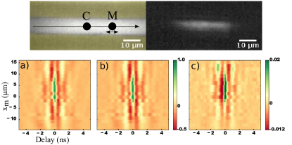
Figure 1: (Color online) Top panels: images of the surface of the extended microcavity laser with integrated saturable absorber below (left) and above (right) laser threshold. The dark (yellow) zone is the gold mask delimiting the pumping region. Bottom panels: a) temporal cross-correlation $X{}_{C,M}(t_{k},x_{m})$ (see text) between the detector responses in points C ($x_{m}=0$) and M at delays $t_{k}=k\Delta t$. b) Same as a) restricted to extreme events at point C. c) Average of the responses at point M and at times where an abnormal event has occurred in the center of the laser in C.

In this Letter, we report on experimental and numerical results on the physics of extreme events appearance in a spatially extended nonlinear dissipative system and establish the origin of this dynamics in the emergence of spatiotemporal chaos. Our system is a planar microcavity laser with integrated saturable absorber Barbay et al. (2005); Elsass et al. (2010a) pumped along a rectangular aperture, implementing a quasi 1D spatially extended nonlinear dissipative system (cf Fig.1). Besides the very different dynamical regimes that can be observed in it (e.g. laser cavity solitons Elsass et al. (2010b, a) or excitable regimes Barbay et al. (2011); Selmi et al. (2014)), a particularity of this system is that in absence of spatial coupling it does not display irregular or aperiodic dynamics and hence extreme events Dubbeldam and Krauskopf (1999). However, spatial coupling through diffraction and nonlinear effects can make the dynamics become more irregular, especially if the system has a large aspect ratio (or Fresnel number) as is the case here. Above the laser threshold, self-pulsing takes place and we study experimentally the impact of the pumping intensity on the intensity statistics and on the occurrence of extreme events. By recording the dynamics simultaneously in two different spatial points we are able to study whether the extreme events occur through a mechanism of coherent structure collision. Indeed, stationary and propagative laser coherent structures were predicted Perrini et al. (2005); Rosanov et al. (2005a, b); Prati, F. et al. (2010); Tissoni et al. (2012); Vladimirov et al. (2014) in this system and stationary structures were observed Elsass et al. (2010b, a) in some parameter regions. With the help of a mathematical model, linear stability and numerical analysis of the dynamics we unveil the dynamical origin of the extreme events found.

The microcavity structure used in this experiment is described in Elsass et al. (2010b, a). A gold mask is deposited onto the sample surface to define the pump geometry. We concentrate on an elongated shaped pump profile with an gold opening gold having 80$\mu$m length and $10\mu$m width. The linear microavity is pumped above threshold and the intensity in a point close to its center is recorded with a fast avalanche photodiode (5GHz bandwith). The temporal signal is amplified thanks to a low noise, high bandwidth amplifier and acquired with a 6GHz oscilloscope at 20GS/s ($\Delta t=50$ps). Up to $50\times 10^{6}$ points can be acquired in a single trace. Figure 1 shows the near field of the laser below and above threshold, respectively.

Time traces once acquired are treated to display the histogram of the intensity heights. Figure 2 displays histograms versus pump parameter. At normalized pump power $P/P_{th}=1.02$, where $P_{th}$ is the pump at laser threshold, they are characterized by a quadratic decay in the tails, and the probability density function (PDF) looks like a Rayleigh distribution for a positive valued Gaussian process. As the pump is increased, the statistics develops long tails with an initial exponential decay ($P/P_{th}=1.17$). For still higher pump values, the PDF becomes exponential ($P/P_{th}=1.20$) and then redisplays Gaussian tails ($P/P_{th}=1.25$). The global evolution of the mean amplitude versus pump intensity is reminiscent of the dynamics expected for a zero-dimensional laser with saturable absorber Tierno et al. (2011) : close to threshold, quite a regular amplitude pulse train sets in (see Figs.2c). For higher pump, the mean pulse period increases and, because of the spatial coupling, the amplitude becomes very irregular and displays a complex dynamics (Figs.2d,g,h). We have computed the threshold amplitude for extreme events adopting the traditional hydrodynamical criterion. We consider as extreme events those events having a height $H$ twice the significant height $H_{s}$ (mean of the highest tertile of the PDF), i.e. with an abnormality index $AI\equiv H/H_{s}>2$ Onorato et al. (2013). The height $H$ is extracted as the maximum of the left and right intensity heights $H=\max(H_{l},H_{r})$. Note that the results do not change significantly by considering either $H$, $H_{l}$ or $H_{r}$. To get rid of the large number of small peaks of noise at the left of the PDF, we compute the significant height $H_{s}$ only by considering events whose height is larger than the observed maximum peak dark noise amplitude which is about 5mV (note that the rms noise is only 0.9mV). This threshold introduces a more stringent criterion for the extreme events detection. Extreme events are depicted in red under the histograms presented in Fig.2. We observe, that the maximum number of extreme events is obtained in the PDF with a non-Gaussian tail, i.e. with a normalized pump of $1.17$.

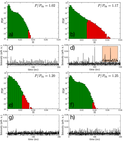
Figure 2: (Color online) a,b,e,f) : Logarithm of the PDF of the intensity height $H$ at position C for different normalized pump values. Extreme events ($AI>2$) are shown in red. c,d,g,h), are excerpts of the time evolution for the corresponding pumps. In d) is plotted a 20ns zoom on the central extreme event.

The statistics of times between two spikes with $AI>2$ displays a Kramers statistics with exponential behavior, marking that spikes appearance obeys a Poisson, memoryless process. We now study the spatiotemporal structure of the statistics of emitted pulses. We record the dynamics in two points, one at a fixed position at the center of the laser (represented by point C) and the other moving along the long line laser (point M). This is made by enlarging the laser surface image by optical magnification and placing the detectors in that plane. On bottom panels in Fig.1, we plot the normalized cross-correlation $X{}_{c,m}(k)$ of the $N=10^{5}$ first recorded points (5$\mu$s) between the signal recorded at the central detector $y_{c}$ at point $C$ and the one at the moving detector $y_{m}$ at location $M$, $1\leq m\leq 20$ such that

$$X{}_{c,m}(k)=\frac{1}{N\sigma_{y_{c}}\sigma_{y_{m}}}\sum_{i}(y_{c}(i)-\bar{y}_{c})(y_{m}(i+k)-\bar{y}_{m})$$

where the bar symbol and $\sigma$ indicate the mean value and the standard deviation. In the central part appears a zone with high positive (green) cross correlation followed and preceded by two bands of negative cross-correlation. The temporal band in which the cross-correlation is nonzero extends about 2ns from around zero delay. Therefore, we can infer the existence of a finite correlation length in the system which is smaller than the lasing system size (about 30$\mu$m). However, since the correlation bands are vertical at these timescales, we cannot evidence clearly propagation effects (at least with the temporal resolution of our setup) though there is a slight bending of the correlated band (in green). In Fig.1b) we restrict the cross-correlation around the points where $AI>2$, i.e. we consider only extreme events. Notice that there are no major differences between the two cross-correlations, hence there seems not to be any statistical marker of the appearance of an extreme event in this regime, and in particular no clear sign of propagation of a coherent structure either. These results indicate that extreme height intensity peaks appear in a spatial correlation zone and disappear almost immediately everywhere in this zone. Correlation is therefore maximum at zero delay for almost all positions detected. Figure 1c) depicts the average of the responses at position $M$ and at times where an abnormal event has occurred in the center of the laser in $C$. The average shows a clear time asymmetry around the correlated structure, every selected event begins with a large amplitude dip followed by a large positive peak. On the wings of the correlated zone we can see another dip. In this system extreme events thus appear and disappear almost simultaneously everywhere in a correlation window. There is no evidence, at least up to our temporal resolution, of clear collision of coherent structures leading to the observed behavior. Instead, we shall consider the complexity in the spatiotemporal dynamics itself as the dynamical origin of extreme events.

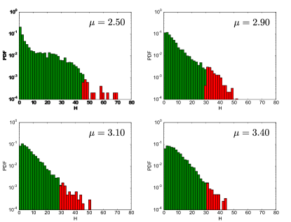
Figure 3: (Color online) Logarithm of the PDF of the theoretical height distribution for the 1D laser with saturable absorber, Eqs.(1), versus pump parameter $\mu$. Extreme events ($AI>2$) are shown in red.

To this aim, we compare our findings with numerical simulations of envelope equation of a one-dimensional spatially extended laser with saturable absorber Bache et al. (2005). The model consists in three coupled nonlinear partial differential equations

$$\frac{\partial E}{\partial t} = \left[(1-i\alpha)G+(1-i\beta)Q-1\right]E+i\frac{\partial^{2}E}{\partial x^{2}}$$

$$\frac{\partial G}{\partial t} = \gamma_{g}\left[\mu-G(1+|E|{}^{2})\right]$$ (1)

$$\frac{\partial Q}{\partial t} = \gamma_{q}\left[-\gamma-Q(1+s|E|^{2})\right]$$

for the intracavity electric-field envelope $E(x,t)$, the carrier density in the gain (resp. saturable absorber) section $G(x,t)$ (resp. $Q(x,t)$). The non-radiative carrier recombination rates are $\gamma_{g}$ and $\gamma_{q}$ with pumping $\mu$ and linear absorption $\gamma$. The Henry enhancement factors in both sections are $\alpha$ and $\beta$, respectively. Diffraction is included through the complex Laplacian term. Time has been rescaled to the field lifetime in the cavity which is calculated to be here $8.0ps$ given the cavity design parameters. Space is rescaled to the diffraction length $w_{d}$ which is $7.4\mu m$. We take parameters compatible with our semiconductor system : $\alpha=2$, $\beta=0$, $s=10$, $\gamma_{g}=\gamma_{q}=0.005$ and $\gamma=0.5$. The equations are simulated using the Xmds2 package Dennis et al. (2013) with a split operator method and an adaptative, fourth-order Runge-Kutta method for time integration. The width of the integration region $w$ is $w/w_{d}=24$ with a top-hat pumping of width $w_{p}/w_{d}=12$. Based on the results developed in Bache et al. (2005), we can describe the main properties of the plane-wave stationary solutions and of the linear stability analysis. The results are shown on Fig. 4 for the latter set of parameters. The plane-wave characteristic curve of the laser has a C-shape with a subcritical bifurcation at threshold for $\mu_{th}=1+\gamma$ provided $s>1+1/\gamma$. In a certain range of parameters, the system also exhibits an Andronov-Hopf bifurcation giving rise to self-pulsation (for $\mu<\mu_{H}\sim 3.08$). When including the spatial degree of freedom, a linear stability analysis reveals that the upper branch is usually Turing unstable everywhere (gray region), giving rise to a complex spatiotemporal dynamics. A Andronov-Hopf instability can also occur for small harmonic perturbations in space with a band of unstable wavevectors $k$ (blue region disconnected from the vertical axis).

The Logarithm of the PDF for the theoretical height distribution for Eqs.(1) is shown in Fig.3. For low pumping it displays a sub-exponential tail with a small number of extreme events. Then the tail of the PDF progressively becomes more and more exponential at the start of the distribution with a large deviation for large events giving rise to a maximum number of extreme events for $\mu=2.9$. The tail of the distribution becomes then quasi exponential at $\mu=3.1$ and then sub-exponential again at $\mu=3.4$ with a decrease of the number of extreme events. These observations reproduce qualitatively well what is found in the experiment. Moreover, the shape of the distribution seems to be strongly correlated to the presence or not of a Andronov-Hopf bifurcation : only when it is present can we observe a heavy tailed distribution. At the transition between the Hopf-Turing and Turing-only region we observe the maximum number of extreme events (for $\mu=2.9$).

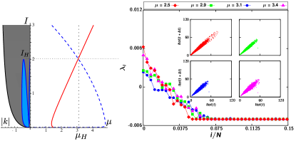
Figure 4: (Color online) Phase portrait of LSA model. Left panel stands for characteristic curve $\mu(I)$ (red) along with the unstable wavevector regions of the the linear stability analysis (Turing instability, grey; Andronov-Hopf instability, blue). Right axis is $\mu$ and left axis is the modulus $|k|$ of the unstable wavevectors. The plane-wave Hopf curve is shown in dashed, blue. Right panel shows the computed Lyapunov spectrum for different pump parameters and corresponding two-dimensional delay-embedding for the total intensity $I_{tot}(t)$.

A characterization of chaos and spatiotemporal chaos can be achieved by means of Lyapunov exponents Manneville (1990). These exponents measure the growth rate of generic small perturbations around of a given trajectory in a finite dimensional dynamical systems. There are as many exponents as the dimension of the system under study. Additional information about the complexity of the system can be obtained from the exponents, for instance the dimension of the strange attractor (spectral dimensionality) or measures of the dynamic disorder (entropy)Ott (2002) or characterization of bifurcations diagram Clerc and Verschueren (2013). The analytical study of Lyapunov exponents is a thorny endeavor and in practice inaccessible. Hence, a reasonable strategy is to derive the exponents numerically by discretizing the set of partial differential equations (1). Let $N$ be the number of discretization points, then the system has $N$ Lyapunov exponents $\lambda_{i}$. If the Lyapunov exponents are sorted in decreasing order and in the thermodynamic limit ($N\to\infty$), these exponents converge to a continuous spectrum as Ruelle conjectured Ruelle (1982). Therefore, if the system has spatiotemporal chaos in this limit, there exists an infinite number of positive Lyapunov exponents. The set of Lyapunov exponents provides an upper limit for the strange attractor dimension through the Kaplan-Yorke dimension Ott (2002) $D_{\mathrm{KY}}=p+\sum_{i-1}^{p}\lambda_{i}/\lambda_{p+1}$, where $p$ is the largest integer that satisfies $\sum_{i-1}^{p}\lambda_{i}>0$ . In the thermodynamic limit the Yorke-Kaplan dimension diverges with the size of the system as a consequence of the Lyapunov density Paul et al. (2007). We have calculated the Lyapunov spectrum (cf. Fig.4) corresponding to the total intensity integrated over x in the model (1). This figure clearly shows that when the system exhibits extreme events it is in a regime of spatiotemporal chaos with several non-zero Lyapunov exponents in the Lyapunov spectrum and an absence of structure in the delay embedding.

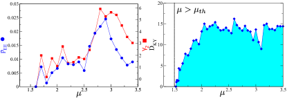
Figure 5: (Color online) Left panel : Proportion of extreme events ($p_{EE}$, blue circles), normed kurtosis ($\gamma_{2}$, red squares) versus pump $\mu$. Right panel : Kaplan-Yorke dimension ($D_{\mathrm{KY}}$, blue diamonds) versus pump $\mu$.

Moreover, we have computed the proportion of extreme events $p_{EE}$, the normed kurtosis $\gamma_{2}=\mathbb{E}\left[\left(\left(X-\mu\right)/\sigma\right)^{4}\right]-3$ and the Kaplan-Yorke dimension $D_{\mathrm{KY}}$ versus pump in Fig.5. $p_{EE}$ and $\gamma_{2}$ both display a maximum versus pump around $\mu\simeq 3$ with some correlated oscillations. $D_{\mathrm{KY}}$ increases steadily from zero at $\mu=1.525$ and then saturates after $\mu=2$. From these findings we infer that there is a smooth or supercritical transition of the system into spatiotemporal chaos and this behavior is concomitant with the increase of the number of extreme events. Note however that there is no reason why there should be a strict correlation between $D_{KY}$ and $p_{EE}$ since the latter is related to the structure of the attractor itself and not only to its dimension Lucarini et al. (2014).

In conclusion, we have shown experimental results of extreme events appearance in a quasi-1D broad area laser with saturable absorber. We have analyzed the physical origin of extreme events that occur because of the onset of deterministic spatiotemporal chaos in the system. Irregular dynamics is obviously a prerequisite for the observation of extreme events but we show in our work that the proportion of extreme events is not directly linked to the evolution of the Kaplan-Yorke dimension. A higher dimensional dynamics does not lead necessarily to a higher number of extreme events. The origin of extreme events in that case is thus to be found in the nature of the spatiotemporal complexity that takes place, and thus could offer interesting prospects for control through changing the system geometry or the nature of the coupling.

Acknowlegements

F.S., S.C., Z.L. and S.B. acknowledge partial support from the French network Renatech and the ANR Blanc project Optiroc. M.G.C. thanks for the financial support of FONDECYT projects 1150507.

References

- Nicolis and Nicolis (2012) G. Nicolis and C. Nicolis, Foundations of Complex Systems: Emergence, Information and Prediction, 2nd ed. (World Scientific Publishing Co., Inc., River Edge, NJ, USA, 2012).
- Onorato et al. (2013) M. Onorato, S. Residori, U. Bortolozzo, A. Montina, and F. Arecchi, Physics Reports 528, 47 (2013).
- Kharif and Pelinovsky (2003) C. Kharif and E. Pelinovsky, European Journal of Mechanics - B/Fluids 22, 603 (2003).
- Solli et al. (2007) D. R. Solli, C. Ropers, P. Koonath, and B. Jalali, Nature 450, 1054 (2007).
- Dudley et al. (2008) J. M. Dudley, G. Genty, and B. J. Eggleton, Opt. Express 16, 3644 (2008).
- Mussot et al. (2009) A. Mussot, A. Kudlinski, M. Kolobov, E. Louvergneaux, M. Douay, and M. Taki, Opt. Express 17, 17010 (2009).
- Kibler et al. (2010) B. Kibler, J. Fatome, C. Finot, G. Millot, F. Dias, G. Genty, N. Akhmediev, and J. M. Dudley, Nat Phys 6, 790 (2010).
- Arecchi et al. (2011) F. T. Arecchi, U. Bortolozzo, A. Montina, and S. Residori, Phys. Rev. Lett. 106, 153901 (2011).
- Lecaplain et al. (2012) C. Lecaplain, P. Grelu, J. M. Soto-Crespo, and N. Akhmediev, Phys. Rev. Lett. 108, 233901 (2012).
- Antikainen et al. (2012) A. Antikainen, M. Erkintalo, J. M. Dudley, and G. Genty, Nonlinearity 25, R73 (2012).
- Birkholz et al. (2013) S. Birkholz, E. T. J. Nibbering, C. Brée, S. Skupin, A. Demircan, G. Genty, and G. Steinmeyer, Phys. Rev. Lett. 111, 243903 (2013).
- Pisarchik et al. (2011) A. N. Pisarchik, R. Jaimes-Reátegui, R. Sevilla-Escoboza, G. Huerta-Cuellar, and M. Taki, Phys. Rev. Lett. 107, 274101 (2011).
- Bonatto et al. (2011) C. Bonatto, M. Feyereisen, S. Barland, M. Giudici, C. Masoller, J. R. R. Leite, and J. R. Tredicce, Phys. Rev. Lett. 107, 053901 (2011).
- Montina et al. (2009) A. Montina, U. Bortolozzo, S. Residori, and F. T. Arecchi, Phys. Rev. Lett. 103, 173901 (2009).
- Randoux and Suret (2012) S. Randoux and P. Suret, Opt. Lett. 37, 500 (2012).
- Kovalsky et al. (2011) M. G. Kovalsky, A. A. Hnilo, and J. R. Tredicce, Opt. Lett. 36, 4449 (2011).
- Bosco et al. (2013) A. K. D. Bosco, D. Wolfersberger, and M. Sciamanna, Opt. Lett. 38, 703 (2013).
- Odent et al. (2010) V. Odent, M. Taki, and E. Louvergneaux, Natural Hazards and Earth System Science (2010).
- Marsal et al. (2014) N. Marsal, V. Caullet, D. Wolfersberger, and M. Sciamanna, Opt. Lett. 39, 3690 (2014).
- Bonazzola et al. (2013) C. Bonazzola, A. Hnilo, M. Kovalsky, and J. R. Tredicce, Journal of Optics 15, 064004 (2013).
- Barbay et al. (2005) S. Barbay, Y. Ménesguen, I. Sagnes, and R. Kuszelewicz, Appl. Phys. Lett. 86, 151119 (2005).
- Elsass et al. (2010a) T. Elsass, K. Gauthron, G. Beaudoin, I. Sagnes, R. Kuszelewicz, and S. Barbay, Eur. Phys. J. D 59, 91 (2010a), 10.1140/epjd/e2010-00079-6.
- Elsass et al. (2010b) T. Elsass, K. Gauthron, G. Beaudoin, I. Sagnes, R. Kuszelewicz, and S. Barbay, Appl. Phys. B 98, 327 (2010b), 10.1007/s00340-009-3748-9.
- Barbay et al. (2011) S. Barbay, R. Kuszelewicz, and A. M. Yacomotti, Opt. Lett. 36, 4476 (2011).
- Selmi et al. (2014) F. Selmi, R. Braive, G. Beaudoin, I. Sagnes, R. Kuszelewicz, and S. Barbay, Phys. Rev. Lett. 112, 183902 (2014).
- Dubbeldam and Krauskopf (1999) J. L. A. Dubbeldam and B. Krauskopf, Opt. Commun. 159, 325 (1999).
- Perrini et al. (2005) I. Perrini, S. Barbay, T. Maggipinto, M. Brambilla, and R. Kuszelewicz, Appl. Phys. B: Lasers Opt. 81, 905 (2005), 10.1007/s00340-005-2030-z.
- Rosanov et al. (2005a) N. Rosanov, S. Fedorov, and A. Shatsev, Appl. Phys. B 81, 937 (2005a).
- Rosanov et al. (2005b) N. N. Rosanov, S. V. Fedorov, and A. N. Shatsev, Phys. Rev. Lett. 95, 053903 (2005b).
- Prati, F. et al. (2010) Prati, F., Tissoni, G., Lugiato, L. A., Aghdami, K. M., and Brambilla, M., Eur. Phys. J. D 59, 73 (2010).
- Tissoni et al. (2012) G. Tissoni, K. Aghdami, M. Brambilla, and F. Prati, The European Physical Journal Special Topics 203, 193 (2012).
- Vladimirov et al. (2014) A. G. Vladimirov, A. Pimenov, S. V. Gurevich, K. Panajotov, E. Averlant, and M. Tlidi, Philosophical Transactions of the Royal Society of London A: Mathematical, Physical and Engineering Sciences 372 (2014), 10.1098/rsta.2014.0013.
- Tierno et al. (2011) A. Tierno, N. Radwell, and T. Ackemann, Phys. Rev. A 84, 043828 (2011).
- Bache et al. (2005) M. Bache, F. Prati, G. Tissoni, R. Kheradmand, L. Lugiato, I. Protsenko, and M. Brambilla, Appl. Phys. B 81, 913 (2005).
- Dennis et al. (2013) G. R. Dennis, J. J. Hope, and M. T. Johnsson, Computer Physics Communications 184, 201 (2013).
- Manneville (1990) P. Manneville, in Dissipative Structures and Weak Turbulence, edited by P. Manneville (Academic Press, Boston, 1990).
- Ott (2002) E. Ott, Chaos in dynamical systems (Cambridge University Press, Cambridge, New York, 2002).
- Clerc and Verschueren (2013) M. G. Clerc and N. Verschueren, Phys. Rev. E 88, 052916 (2013).
- Ruelle (1982) D. Ruelle, Commun. Math. Phys 87, 287 (1982).
- Paul et al. (2007) M. R. Paul, M. I. Einarsson, P. F. Fischer, and M. C. Cross, Phys. Rev. E 75, 045203 (2007).
- Lucarini et al. (2014) V. Lucarini, D. Faranda, J. Wouters, and T. Kuna, Journal of Statistical Physics 154, 723 (2014).