Quasi-Newton Approach for an Atmospheric Tomography Problem

Abstract

This work studies the usage of well-known smoothed total variation regularization for solving an atmospheric tomography problem named as GPS-tomography in some quasi-Newton methods. That is we solve an unconstrained, convex, smooth minimization problem associated with a general type Tikhonov functional containing smoothed form of total variation penalty term by quasi-Newton methods. As a result of the conducted experiments, on the basis of error analysis i.e. convergence analysis, it is concluded that the limited memory BFGS algorithm with trust region is the most effective algorithm in terms obtaining a reasonable optimum solution.

Keywords. smooth total variation, GPS-Tomography, refractivity profile, limited memory BFGS, trust region

1 Introduction

One important predictor in meteorology is the humidity of the atmosphere. This is estimated by fan-beam measurements between satellite transmitters and land-based receivers. The measurements are sparse and fluctuate randomly with receiver availability. The task is to reconstruct from these measurements the 3-dimensional, spatially varying index of refraction of the atmosphere, from which the relative humidity can be inferred.

GPS-tomography involves the reconstruction of some quantity, pointwise within a volume (e.g. humidity) from geodesic X-ray measurements transmitted by nonuniformly distributed transducers (satellites). These measurements are collected by nonuniformly distributed receivers on the ground (ground stations). As with conventional tomography, the task here is the reconstruction of the density volume profile of a layer in the atmosphere from a set of line integrals. Function reconstruction from its measured line integrals was firstly proposed and solved in [36]. Profound mathematical and numerical aspects of the computerized tomography have been studied in [29, 31]. Measurement from the Radon transform is obtained by integrating some integrable function over the hyperplanes in $\mathbb{R}^{N}.$ The ray transform, on the other hand, produces measurement by integrating the function over straight lines. It is known that in the two dimensional tomography, general Radon and ray transformations coincide, [31, p. 17].

In the discretized form of the problem, it is assumed that each station receives equal number of signals transmitted by the satellites. Also for the sake of simplicity, we ignore any deviations from the shortest path between transmitters and receivers due to atmospheric refractivity. The received signal is then modelled as a line integral along the shortest path between the satellites and the ground stations.

Peculiar to this problem, reconstructions by Kalman filtering and ART have been widely applied, [4, 27, 35, 46]. Different from these conventional numerical reconstruction methods, we propose a quasi-Newton approach. One of the effective quasi-Newton methods is limited memory BFGS (L-BFGS) algorithm which is particularly suggested by this work. The L-BFGS algorithm has been also applied for atmospheric imaging wherby the forward problem has been modelled as a phase retrieval problem, see [43]. We, on the other hand, consider the forward model as a linear atmospheric transmission problem which is a straight line approximation. This means that despite the refractivity in the microwave signals while traversing the troposphere layer of the atmosphere, we ignore attenuation. The unknown function is denoted by $\varphi$ which is assumed to be in the class of some reflexive Banach space ${\mathcal{V}}={\mathcal{L}}^{p}(\Omega),$ for $1\leq p\leq d/(d-1)$ where $d=3$ since this work focuses on three dimensional reconstruction. The measured noisy data is assumed to be in the class of some Hilbert space ${\mathcal{H}}.$ We, then, seek the minimizer for some general Tikhonov objective functional given in the form of

$$F_{\alpha}(\varphi,f^{\delta}): {\mathcal{V}}\times{\mathcal{H}} \longrightarrow\mathbb{R}_{+}$$ (1.1)

$$(\varphi,f^{\delta}) \longmapsto F_{\alpha}(\varphi,f^{\delta}):=\frac{1}{2}||{\mathcal{T}}\varphi-f^{\delta}||_{{\mathcal{H}}}^{2}+\alpha J(\varphi),$$

where the forward operator ${\mathcal{T}}:{\mathcal{V}}\rightarrow{\mathcal{H}}$, as will be described soon, is a linear fan-beam projection operator. Here, the penalty term $J:{\mathcal{V}}\rightarrow\mathbb{R}_{+}$ is convex and Fréchet differentiable with the regularization parameter $\alpha>0$ before it.

We demonstrate our regularization on simulated data, employing a novel reverse-communication large-scale nonlinear optimization software SAMSARA which has been developed by D. R. Luke [25]. Comparison between the illustrated results from SAMSARA and the results from traditional lagged diffusivity fixed point iteration algorithm, LDFP in [44, 45], is also provided.

1.1 Physical Problem: From Propagation in Time to Propagation in Space

This is an inverse problem with incomplete data. It is well known that the incompleteness of data causes nonuniqueness issue in inverse problems, [31, p. 144]. Particularly in tomography, the assumption of compact support is essential in order for unique solvabilibility. In other words, problems characterizing incomplete data case are uniquely solvable if the unknown function $\varphi$ has compact support. In this subsection, although it does not completely overlap the reality, we will model the physical problem with the geometrical assumption of compact support. Firstly, just by the nature of the physical problem, $\varphi$ is not a constant function and contains smooth intensity. Formulation of the simulated profile is presented in Subsection 3.2. Since this work solely aims to provide empirical results for a large scale application problem by some well-known optimizatin and regularization strategies, we will not state any theoretical result. However, still as a duty of any inverse problem research work, formal assumptional statemens on compact support must be made that uniqueness principle is verifiable.

Let $(\rho_{s},\sigma_{s})$ be the polar angles of the station $\mathbf{s}$ as inclination and azimuth respectively. Then in spherical coordinates, the location of any station $\mathbf{s}$ is given by

$$\mathbf{s}=R\left(\begin{array}[]{cccccccccccccccccc}\cos(\rho_{s})\cos(\sigma_{s}),\cos(\rho_{s})\sin(\sigma_{s}),\sin(\rho_{s})\end{array}\right)^{T},$$

where $R=\sqrt{{x_{s}}^{2}+{y_{s}}^{2}+{z_{s}}^{2}}.$ Following [29, Ch. 2] and [33, p. 45], the signal path direction $\vec{\theta}$ is reparametrized by

$$\vec{\theta} = -\left(\begin{array}[]{cccccccccccccccccc}\cos(\rho_{r}+\rho_{s})\cos(\sigma_{r}+\sigma_{s}),\cos(\rho_{r}+\rho_{s})\sin(\sigma_{r}+\sigma_{s}),\sin(\rho_{r}+\rho_{s})\end{array}\right)^{T}$$ (1.3)

$$= -\left(\begin{array}[]{cccccccccccccccccc}\cos(\tilde{\rho})\cos(\tilde{\sigma}),\cos(\tilde{\rho})\sin(\tilde{\sigma}),\sin(\tilde{\rho})\end{array}\right)^{T},$$ (1.5)

where the inclination and the azimuth of the signal path according to the surface are denoted by $(\rho_{r}+\rho_{s},\sigma_{r}+\sigma_{s})=(\tilde{\rho},\tilde{\sigma}),$ see Figure 2 for this angular parameterization.

Let $g$ be some Lipschitz continuous function with its Lipschitz constant $L_{g}\in\mathbb{R}_{+}$ for the surface of the earth,

$$g:[0,S]\times[0,P]\rightarrow[0,h^{\infty}),$$ (1.6)

and denote by ${\mathcal{G}}$ the graph of the surface function $g$

$${\mathcal{G}}=\mathrm{graph}(g):=\{(x,y,z)\mbox{ }|\mbox{ }(x,y)\in[0,S]\times[0,P],z=g(x,y)\geq 0\}.$$ (1.7)

A ground station $\mathbf{s}$ is a set of points in $\mathbb{R}^{3}$ located on earth with the coordinate points $(x_{s},y_{s},z_{s}),$

$$\mathbf{s}:=(x_{s},y_{s},z_{s})\in{\mathcal{G}},$$ (1.8)

and likewise emitters $\mathbf{e}$ that are all located at the same altitude $h^{\infty}$ is also set of points in $\mathbb{R}^{3},$

$$\mathbf{e}:=\{(x_{e},y_{e},z_{e})\mbox{ }|\mbox{ }(x_{e},y_{e})\in[0,S]\times[0,P]\mbox{ and }z_{e}=h^{\infty}\}.$$ (1.9)

Our area of interest is a compact subdomain, i.e. $\Omega\subset\Omega_{o},$

$$\Omega_{o}:=\left\{(x,y,z)\in[0,S]\times[0,P]\times[0,h^{\infty}]\mbox{ }|\mbox{ }z\geq g(x,y)\right\}.$$ (1.10)

Obviously, the definitions in (1.7) and (1.10) both imply ${\mathcal{G}}\subset\Omega_{o}.$

Since we consider our network as straight line approximation, that is we do not include attenuation, we model each signal path as a ray in $\mathbb{R}^{3}.$ There can be formulated a linear parameter function $t:\mathbb{R}\rightarrow\mathbb{R},$ $t(\epsilon):=\frac{\epsilon}{\sin{(\tilde{\rho})}},$ such that a ray in $\mathbb{R}^{3}$ starting from the station $\mathbf{s}$ in the direction $\vec{\theta}\in\mathbb{S}^{2}$ is defined by

$$\gamma_{[\mathbf{s},\vec{\theta}]}(\epsilon):=\left\{\mathbf{s}+\frac{\epsilon}{\sin{(\tilde{\rho})}}\vec{\theta}\mbox{ }\Bigg{|}\mbox{ }\epsilon\in[z_{s},h^{\infty}]\right\}.$$ (1.11)

Here, in fact, $\gamma$ is the minimal path between any two points in $\mathbb{R}^{3}.$ So, a microwave signal takes the least time $T$ with speed $c$ along this path

$$T=\frac{1}{c}\int_{\bf{r}\in\gamma}{n(\bf{r})}d\bf{r},$$ (1.12)

where $n$ is index of refraction. The linear relation between the refractivity profile $N$ and the refractive index $n$ is expressed by $N=10^{6}(n-1),$ [4, 27, 46]. Thus, if one chooses the refractivity profile as the frame of reference, then (1.12) reads

$$T=\frac{1}{c}\int_{\bf{r}\in\gamma}(10^{-6}{N(\bf{r})}+1)d\bf{r}.$$ (1.13)

To obtain measurement $f,$ we apply fan-beam projection operator along the ray $\gamma_{[\mathbf{s},\vec{\theta}]}$ on some density profile defined by $\varphi:=\frac{1}{c}\left(10^{-6}N+1\right)=\frac{n}{c}.$ The unknown density function $\varphi:\Omega\rightarrow\mathbb{R}$ is assumed to be integrable and, by convention, vanishes outside the area of interest $\Omega.$ This is explained by introducing a step function as such

$$\tilde{\varphi}(x):=\left\{\begin{array}[]{rcl}\varphi(x)&\mbox{, for}&x\in\Omega\\ 0&\mbox{, for}&x\in\Omega_{o}\backslash\Omega.\end{array}\right.$$ (1.16)

Physically, there exist many rays in various directions $\vec{\theta}\in\mathbb{S}^{2}.$ However, the measured data can only be obtained through the rays which do not have empty intersection with the area of interest $\Omega.$ Let ${\mathcal{Z}}$ be the domain of the integrated measurement which is the function of station $\mathbf{s}$ and directional vector $\vec{\theta}.$ Denote by

$$\mathbb{S}_{\mathbf{s}}:=\{\vec{\theta}\in\mathbb{S}^{2}|(\mathbf{s},\vec{\theta})\in{\mathcal{Z}}\},$$ (1.17)

the set of intercepted directions where the domain of the integrated measurement through one ray $\gamma_{[\mathbf{s},\vec{\theta}]}$ can be presented by

$$f:{\mathcal{Z}}={\mathcal{D}}(f)\subset{\mathcal{G}}\times\mathbb{S}_{\mathbf{s}}\rightarrow\mathbb{R}_{+},$$ (1.18)

with

$${\mathcal{D}}(f):=\{(\mathbf{s},\vec{\theta})\mbox{ }|\mbox{ }\tilde{\rho}\geq|\arctan(L_{g})|,\pi-\tilde{\rho}>0\mbox{ , and }\gamma_{[\mathbf{s},\vec{\theta}]}\cap\Omega\neq\emptyset\}.$$ (1.19)

By (1.19), one must understand that the slope of the ray cannot be larger than the elevation angle $\tilde{\rho}.$ Furthermore, rays that are parallel to the surface are not taken into account for the measurement. There could also be rays that do not intersect with the area of interest $\Omega.$ Therefore, we are only interested in the rays that have no empty intersection with $\Omega,$

$$\gamma_{[\mathbf{s},\vec{\theta}]}\cap\Omega\neq\emptyset\mbox{, for }\theta\in\mathbb{S}_{\mathbf{s}}\subset\mathbb{S}^{2}\mbox{, }\mathbf{s}\in{\mathcal{G}}\subset\Omega_{o}.$$

Then, in fact, the measured data $f({\mathbf{s}},\vec{\theta})$ is obtained only for $\vec{\theta}\in\mathbb{S}_{\mathbf{s}}.$ Note that $\mathbb{S}_{\mathbf{s}}\subset\mathbb{S}^{2},$ which is the partial information case. Thus collection of the measurement operation, in light of fan-beam projection principle, is formulated by

$$f(\mathbf{s},\vec{\theta})={\mathcal{T}}_{\mathbf{s}}\varphi(\vec{\theta})=({\mathcal{T}}\varphi)(\mathbf{s},\vec{\theta})=\int_{\gamma_{[\mathbf{s},\vec{\theta}]}}\varphi(\mathbf{r})d\mathbf{r},\mbox{ for }\mathbf{r}\in\gamma_{[\mathbf{s},\vec{\theta}]}\subset\Omega_{o}.$$ (1.20)

Also, with the angular parameterization introduced above, we then have

$${\mathcal{T}}_{\mathbf{s}}\varphi(\vec{\theta})={\mathcal{T}}\varphi(\tilde{\rho},\tilde{\sigma}),\mbox{ for }(\tilde{\rho},\tilde{\sigma})\in(0,\pi)\times(0,2\pi).$$

According to [19, Theorems 5.1 - 5.6] and [31, Theorem 6.2] the linear transformation (1.20) is injective only under compact support assumption and in the presence of directional vectors from the set of intercepted directions, $\theta\in\mathbb{S}_{\mathbf{s}}.$ It is not possible to reconstruct the unknown function $\varphi$ exactly from finitely number of measurements. However, [19, Theorems 5.1 - 5.6] show that arbitrarily good approximation can be obtained.

The discretized integration from one point to the next one along the ray $\gamma$ is carried out via the parameter function $t(\epsilon)=\frac{\epsilon}{\sin{(\tilde{\rho})}},$ for any $\epsilon\in[z_{s},h^{\infty}],$ see Figure 2. In the continuum form, we use ray transform in the direction $\vec{\theta}(\tilde{\rho},\tilde{\sigma})\in\mathbb{S}_{\mathbf{s}}$ for any angle pairs $(\tilde{\rho},\tilde{\sigma}),$ on the density function $\varphi:\Omega\subset\mathbb{R}^{3}\rightarrow\mathbb{R}_{+}$ as such

$$f(\mathbf{s},\vec{\theta})={\mathcal{T}}_{\mathbf{s}}\varphi(\vec{\theta})=({\mathcal{T}}\varphi)(\mathbf{s},\vec{\theta})=\int_{\mathbf{r}\in\gamma_{[\mathbf{s},\vec{\theta}]}}\varphi({\mathbf{r}})d\mathbf{r}=\int_{z_{s}}^{h^{\infty}}\varphi(\gamma_{[\mathbf{s},\vec{\theta}]}(\epsilon))|\gamma^{\prime}_{[\mathbf{s},\vec{\theta}]}(\epsilon)|d\epsilon,$$ (1.21)

where

$$|\gamma^{\prime}_{[\mathbf{s},\vec{\theta}]}(\epsilon)|=\left|\frac{\vec{\theta}}{\sin{(\tilde{\rho})}}\right|,\mbox{ with }|\vec{\theta}|=1.$$ (1.22)

The representation (1.21) is comparable with its nonlinear counterpart in [40, Eq. (1.3)]. So as a linear operator equation, we have ${\mathcal{T}}\varphi=f$ where ${\mathcal{T}}$ represents the line integration operating on the density profile $\varphi$ to obtain measurement $f.$

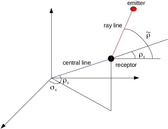
Figure 1: The sketch of angular parameterization. Intersection point between the central and the ray lines is the receptor with the angles $(\rho_{s},\sigma_{s}).$ Emitter is located at the highest altitude $h^{\infty}.$ Its elevation angle according to the surface is denoted by $\tilde{\rho}.$

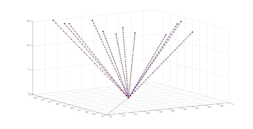
Figure 2: Finitely number of points denoted by blue stars along $12$ rays are illustrated. These points are found via the parameter function $t(\epsilon)=\frac{\epsilon}{\sin{(\tilde{\rho})}},$ for $\epsilon\in[z_{s},h^{\infty}]$ where $h^{\infty}$ is the upper bound of the line integral in (1.21).

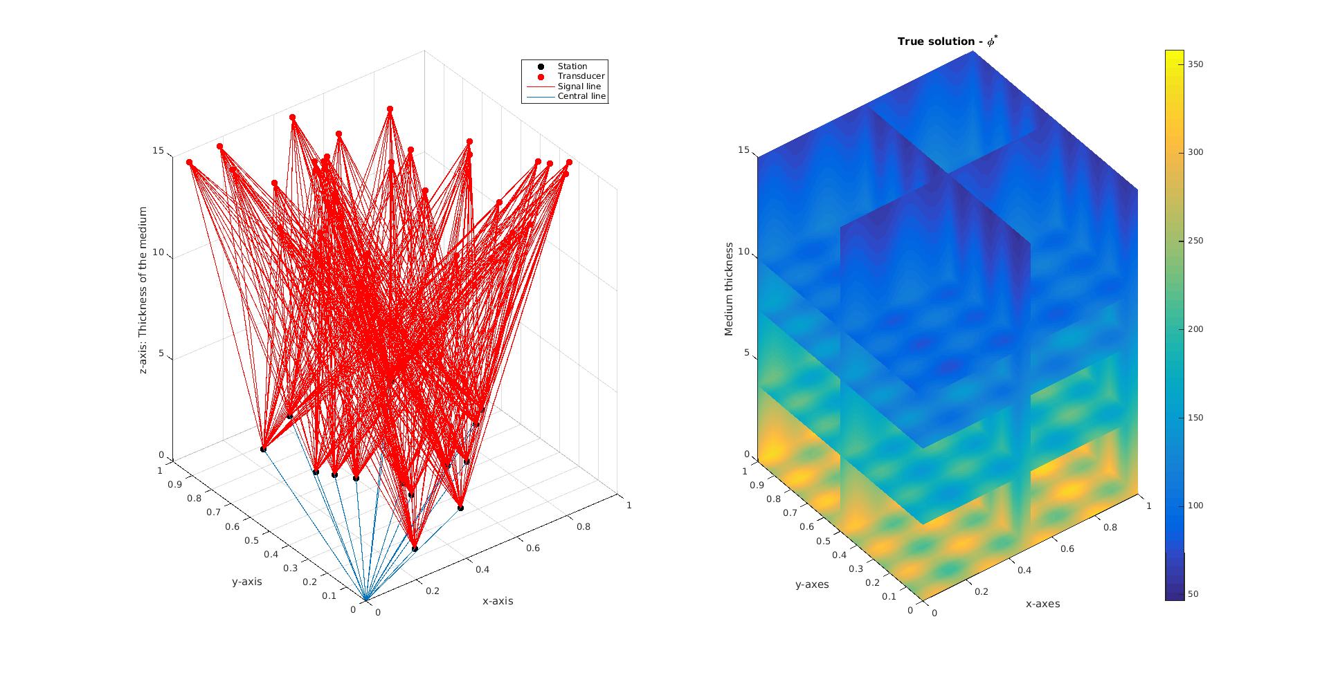
Figure 3: A 3-D network together with simulated data $\varphi,$ as the true solution $\varphi^{\dagger},$ is illustrated over a non-uniformly scaled domain. Black dots indicate stations whilst signals penetrate the area of interest through red dots. In this illustration, $15$ ground stations (receiver) intercept signals emitted by $30$ transducers and all are randomly distributed over $27000$ grid nodes.

2 Minimization Problem, Existence and Uniqueness of the Regularized Solution

It has been conveyed that the use of $TV$ promotes sparsity of the gradient, [5]. In our numerical illustrations, we have simulated a data with smooth intensity, see Subsection 3.2. The weak formulation of TV of some function $\varphi$ defined over the compact domain $\Omega$ is given below.

Definition 2.1.

[$TV(\varphi,\Omega)$][39, Definition 9.64] Over the compact domain $\Omega,$ total variation of a function $TV(\varphi,\Omega)$ is defined in the weak sense as follows ,

$$TV(\varphi,\Omega):=\sup_{\Phi\in{\mathcal{C}}_{c}^{1}(\Omega)}\left\{\int_{\Omega}\varphi(x){\rm div\;}\Phi(x)dx\mbox{ }:\mbox{ }||\Phi||_{\infty}\leq 1\right\}.$$ (2.1)

Total variation type regularization targets the reconstruction of bounded variation (BV) class of functions that are defined by

$$BV(\Omega):=\{\varphi\in{\mathcal{L}}^{1}(\Omega):TV(\varphi,\Omega)<\infty\},$$ (2.2)

endowed with the norm

$$||\varphi||_{BV}:=||\varphi||_{{\mathcal{L}}^{1}}+TV(\varphi,\Omega).$$ (2.3)

BV function spaces are Banach spaces, [44]. By the result in [1, Theorem 2.1], it is known that one can arrive, with a proper choice of $\Phi\in{\mathcal{C}}_{c}^{1}(\Omega),$ in the following from (2.1),

$$TV(\varphi)=\int_{\Omega}|\nabla\varphi(x)|dx\cong\int_{\Omega}\left(|\nabla\varphi(x)|^{2}+\beta\right)^{1/2}dx,$$ (2.4)

where $0<\beta<1$ is fixed and the classical Euclidean norm is denoted by $|\cdot|.$ We also refer [6, 8, 14, 37, 45] where the smoothed form of (2.4) has appeared.

With this theoretical motivation having stated, we are tasked with constructing the regularized solution $\varphi_{\alpha}^{\delta}$ over some compact and convex domain $\Omega\subset{\mathcal{R}}^{3}$ by solving the following smooth, unconstrained, minimization problem,

$$\varphi_{\alpha}^{\delta}\in{\rm arg\,min}_{\varphi\in{\mathcal{V}}}\left\{\frac{1}{2}||{\mathcal{T}}\varphi-f^{\delta}||_{{\mathcal{H}}}^{2}+\alpha J_{\beta}^{\mathrm{TV}}(\varphi)\right\},$$ (2.5)

with its regularization parameter $\alpha>0$ and for the penalty term $J_{\beta}^{\mathrm{TV}}:{\mathcal{V}}\rightarrow\mathbb{R}_{+},$ where in particular ${\mathcal{V}}={\mathcal{W}}^{1,p}$ for $1\leq p\leq d/(d-1)$ and $d=3,$ defined by

$$J_{\beta}^{\mathrm{TV}}(\varphi):=\int_{\Omega}\sqrt{|\nabla\varphi(x)|^{2}+\beta}d{\bf x}.$$ (2.6)

It is the obvious property of the chosen penalty term that $J_{\beta}^{\mathrm{TV}}\in C^{\infty}({\mathcal{V}}).$ Existence and uniqueness of the solution $\varphi_{\alpha}^{\delta}$ for the problem (2.5) has been studied extensively in [1]. By the given facts of our forward operator, one of which is that there could be rays with empty intersection, it can be stated that

$${\mathcal{T}}1\neq 0\mbox{, and }{\mathcal{T}}1\geq 0.$$ (2.7)

This implies the $BV$ coercivity of the objective functional $F_{\alpha}$ from which the existence of the regularized solution is guaranteed. Uniqueness of the solution is simply the consequence of the strict convexity $F_{\alpha}$ which is implied by the injectivity of the forward operator ${\mathcal{T}}.$

3 Discretized Form of the Minimization Problem and the Toy Model Setup

In the computerized environment we always work with finite dimensional setup, thus we only collect discrete data. So, we now introduce our tomographic application and the minimization problems with their components in the finite dimension. We consider the domain $\Omega=[0,1]\times[0,1]\times[0,15]$ and the meshsize $\Delta_{{\bf x}}=1/(N-1)$ with some determined mesh point number $N\in\mathbb{N}$ for any point ${\bf x}=(x,y,z)\in\Omega\subset\mathbb{R}^{3}.$ Note that, here $h^{\infty}=15$ according to (1.21). Within our compact domain $\Omega\subset\mathbb{R}^{3},$ we then generate a point-to-point discretization by starting from some point ${\bf x}_{i-1}\in\Omega\subset\mathbb{R}^{3}$ and iterating onward as such

$${\bf x}_{i}={\bf x}_{i-1}+\Delta_{{\bf x}},\mbox{ for each }i=2,\cdots,N.$$

In our experiments, we have developed $N_{x}=N_{y}=N_{z}=30$ nodes. In the toy model, the speed of light is taken as $c=1,$ see (1.12), in order to be able to measure the propagation of the light beams in space instead of in time. Recall from the Section 1.1 by (1.21) that the electromagnetic signals with the angles $(\rho_{r},\sigma_{r})$ arrive in any receiver $\mathbf{s}$ with the polar angles $(\rho_{s},\sigma_{s})$ in various directions $\mathbf{\theta}\in\mathbb{S}^{2}.$ So the ray path in $\mathbb{R}^{3}$ is the set

$$\gamma_{[\mathbf{s},\theta]}(\epsilon):=\left\{\mathbf{s}+\frac{\epsilon}{\sin{(\tilde{\rho})}}\theta\hskip 2.84544pt\Bigg{|}\hskip 2.84544pt\epsilon\in[z_{s},h^{\infty}]\right\},$$ (3.1)

and the integral transformation that is used for data collection

$$f(\mathbf{s},\theta)={\mathcal{T}}_{\mathbf{s}}\varphi(\theta)=({\mathcal{T}}\varphi)(\theta,\mathbf{s})=\int_{\mathbf{r}\in\gamma_{[\mathbf{s},\theta]}}\varphi({\bf{r}})d\mathbf{r}=\int_{z_{s}}^{h^{\infty}}\varphi(\gamma_{[\mathbf{s},\vec{\theta}]}(\epsilon))|\gamma^{\prime}_{[\mathbf{s},\vec{\theta}]}(\epsilon)|d\epsilon.$$

The full path of the signal is the sum of the paths in the intercepted grid nodes. The model can be interpreted as a system of linear equations. Let us denote the discretized integration by $T.$ With additive white Gaussian noise model vector $z_{j}\sim{\mathcal{N}}(0,1)$ (cf. [22]) and some known noise level $\delta,$ we produce measurement vector by

$$[T\varphi]_{j}=\sum_{i=1}^{N}\varphi_{i}w_{i,j}=f_{j}^{\dagger}+\delta z_{j}=f_{j}^{\delta},$$ (3.2)

where $j=1,2,\cdots S,$ $S$ is the total number of signal paths from all visible satellites in the network at a fixed time instant, $N$ is the total number of grid nodes, $w_{i,j}$ is the length of $j^{th}$ ray passing through the node $i,$ the $\varphi_{i}$ is interpreted as the density of the corresponding $i$th node, [27].

The parameter function $t(\epsilon)=\frac{\epsilon}{\sin{(\tilde{\rho})}}$ in (3.1) permits one to determine the points along each signal for any $\epsilon\in[z_{s},h^{\infty}]$ where $h^{\infty}$ is the upper boundary of the medium as well as the line integral in (1.21), see Figure 2.

Regarding the discretized form of our minimization problem (2.5) with its components, we are provided with the compact forward operator $T:\mathbb{R}^{N}\rightarrow\mathbb{R}^{M}$ and the measurement vector $f^{\delta}\in\mathbb{R}^{M}.$ With this information, our cost functional is then $F_{\alpha}(\varphi,f^{\delta}):\mathbb{R}^{M\times N}\rightarrow\mathbb{R}_{+},$ and we seek for the optimum solution to the problem

$$\varphi_{\alpha}^{\nu+1}\in{\rm arg\,min}_{\varphi^{\nu}\in\mathbb{R}^{N}}\left\{\frac{1}{2}||T\varphi^{\nu}-f^{\delta}||_{2}^{2}+\alpha J(\varphi^{\nu})\right\}.$$ (3.3)

Since we have focused on the smoothed form of the total variation regularization in our analysis, we then define the smooth-TV penalty by

$$J_{\beta}^{\mathrm{TV}}(\varphi^{\nu}):=\sum_{i=1}^{n_{x}}\sum_{j=1}^{n_{y}}\sum_{k=1}^{n_{z}}\Gamma_{\beta}\left((D_{ijk}^{x}\varphi^{\nu})^{2}+(D_{ijk}^{y}\varphi^{\nu})^{2}+(D_{ijk}^{z}\varphi^{\nu})^{2}\right)\Delta_{x}\Delta_{y}\Delta_{z},$$ (3.4)

where the smoothing functional $\Gamma_{\beta}(\Phi):=\sqrt{|\Phi|^{2}+\beta}$ for some fixed $\beta\in(0,1)$ and the discretized spatial derivatives according to the central difference form

$$D_{ijk}^{x}\varphi=\frac{\varphi_{i+1,j,k}^{\nu}-\varphi_{i-1,j,k}^{\nu}}{2\Delta_{x}},\hskip 8.5359ptD_{ijk}^{y}\varphi=\frac{\varphi_{i,j+1,k}^{\nu}-\varphi_{i,j-1,k}^{\nu}}{2\Delta_{y}},\hskip 8.5359ptD_{ijk}^{z}\varphi=\frac{\varphi_{i,j,k+1}^{\nu}-\varphi_{i,j,k-1}^{\nu}}{2\Delta_{z}}.$$ (3.5)

The optimum solution $\varphi_{\alpha}^{\nu}$ must satisfy the first optimality condition. That is

$$0=\nabla F_{\alpha}(\varphi_{\alpha}^{\nu},f^{\delta})=T^{\ast}(T\varphi_{\alpha}^{\nu}-f^{\delta})+\alpha\nabla J_{\beta}^{\mathrm{TV}}(\varphi_{\alpha}^{\nu}).$$

Here $\nabla J_{\beta}^{\mathrm{TV}}(\varphi)$ is calculated by $\frac{d}{dt}J_{\beta}^{\mathrm{TV}}(\varphi+t\Psi)|_{t=0}$ in the direction $\Psi\in{\mathcal{C}}_{c}^{1}(\Omega)$ such that $||\Psi||\leq 1.$ It can be observed that $\nabla J_{\beta}^{\mathrm{TV}}(\varphi)=L(\varphi)\varphi$ with the nonlinear term $L(\varphi),$

$$L(\varphi) = D_{x}^{T}diag(\Gamma^{{}^{\prime}}(\varphi))D_{x}+D_{y}^{T}diag(\Gamma^{{}^{\prime}}(\varphi))D_{y}+D_{z}^{T}diag(\Gamma^{{}^{\prime}}(\varphi))D_{z}$$ (3.13)

$$= \left(\begin{array}[]{cccccccccccccccccc}D_{x}^{T}&D_{y}^{T}&D_{z}^{T}\end{array}\right)\left(\begin{array}[]{cccccccccccccccccc}diag(\Gamma^{{}^{\prime}}(\varphi))&0&0\\ 0&diag(\Gamma^{{}^{\prime}}(\varphi))&0\\ 0&0&diag(\Gamma^{{}^{\prime}}(\varphi))\end{array}\right)\left(\begin{array}[]{cccccccccccccccccc}D_{x}\\ D_{y}\\ D_{z}\end{array}\right).$$

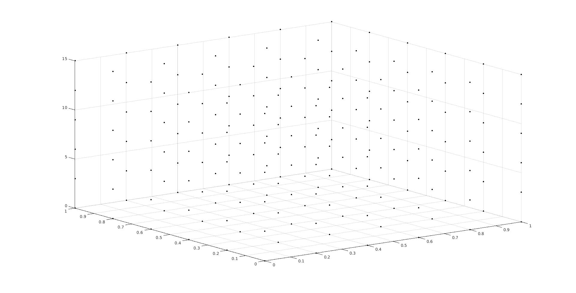
Figure 4: Discretization of our area of interest. For illustration purpose, we only present $6\times 6\times 6$ grid nodes.

3.1 Empirical convergence analysis

Recall that we aim to obtain approximate regularized solution by solving the unconstrained, smooth minimization problem

$$\varphi_{\alpha}^{\delta}\in{\rm arg\,min}_{\varphi\in{\mathcal{V}}}\frac{1}{2}||{\mathcal{T}}\varphi-f^{\delta}||_{{\mathcal{H}}}^{2}+\alpha J_{\beta}^{\mathrm{TV}}(\varphi),$$

with the smooth-TV penalty term

$$J_{\beta}^{\mathrm{TV}}(\varphi):=\int_{\Omega}\sqrt{|\nabla\varphi(x)|^{2}+\beta}dx.$$

Thus, we must observe sufficient decay in the following components that we can claim the optimum solution as a result of any algorithm;

• $F(\varphi_{\alpha}^{\nu},f^{\delta});$ the functional value at every updated point $\varphi_{\alpha}^{\nu},$

• $||\varphi_{\alpha}^{\nu}-\varphi_{\alpha}^{\nu-1}||;$ norm of the succesive iterations at each iteration step $\nu=1,2,\cdots,$

• $\frac{||\varphi_{\alpha}^{\nu}-\varphi^{\dagger}||}{||\varphi^{\dagger}||};$ the relative error value of the reconstruction against the true solution $\varphi^{\dagger},$

• $\|\nabla F(\varphi_{\alpha}^{\nu})\|;$ the norm of the gradient value of the functional at every updated point $\varphi_{\alpha}^{\nu},$

• $\|{\mathcal{T}}\varphi_{\alpha}^{\nu}-f^{\delta}\|;$ the discrepancy of the image of the solution against the given data $f^{\delta}.$

It is expected from the chosen regularization strategy that this strategy must produce a reliable regularized minimizer $\varphi_{\alpha}^{\delta}.$ This reliability is tested in the framework of convergence concept. In order to be able to speak about the convergence of the regularized minimizer (the solution) $\varphi_{\alpha}^{\delta},$ there must be some reference solution to which the regularized solution will approximately converge during the iteration. Likewise in many inverse problems research works, we choose our reference solution as the true solution $\varphi^{\dagger}.$ Convergence of the regularized solution $\varphi_{\alpha}^{\delta}$ to the true solution $\varphi^{\dagger}$ in the Hilbert norm sense $||\varphi_{\alpha}^{\delta}-\varphi^{\dagger}||_{{\mathcal{H}}}$ by some rule for the choice of regularization parameter has been studied and established well, see [15], [21], [23] for the details. This convergence is also known as the total error and is defined by

$$E(\varphi_{\alpha}^{\delta},\varphi^{\dagger}):=||\varphi_{\alpha}^{\delta}-\varphi^{\dagger}||_{{\mathcal{H}}}.$$

From this presentation, one must expect from the numerical experiments that the most reliable solution will be provided by the algorithm which gives the least total error value during the iteration. Aside from the convergence analysis in the pre-image space, we will also focus on the convergence in the image space by analysing the discrepancy between ${\mathcal{T}}\varphi_{\alpha}^{\delta}$ and the measured data $f^{\delta},$ i.e. $||{\mathcal{T}}\varphi_{\alpha}^{\delta}-f^{\delta}||_{{\mathcal{L}}^{2}({\mathcal{Z}})}.$ According to well-known Morozov’s discrepancy principle (MDP), one must define a rule for the choice of the regularization parameter in a way such that the following, with some fixed $1<\underline{\tau}\leq\overline{\tau}<\infty,$

$$\alpha(\delta,f^{\delta})\in\{\alpha>0\mbox{ }:\mbox{ }\underline{\tau}\delta\leq||{\mathcal{T}}\varphi_{\alpha(\delta,f^{\delta})}^{\delta}-f^{\delta}||_{{\mathcal{L}}^{2}({\mathcal{Z}})}\leq\overline{\tau}\delta\}\mbox{ for all given }(\delta,f^{\delta}),$$ (3.14)

must hold. Our tests do not involve any implementation of the discrepancy principle. However, it is still in the expectations of our tests that after some some number of iteration steps, the convergence rate $||{\mathcal{T}}\varphi_{\alpha}^{\delta}-f^{\delta}||_{{\mathcal{L}}^{2}({\mathcal{Z}})}$ in the image space is expected to remain constant.

The updated reconstruction $\varphi_{\alpha}^{\nu}$ will be produced by different gradient based algorithms, see Section 4.1 for the details. Thus, significant decay in the norm of the gradient of the functional is expected, i.e. $\|\nabla F(\varphi_{\alpha}^{\nu})\|\leq\|\nabla F(\varphi_{\alpha}^{\nu-1})\|$ at each iteration step $\nu=1,2,\cdots.$

3.2 The synthetic profile

The atmospheric physical facts behind the refractivity profile of humidity fields can be found in [24, 35]. The vertical profile of the refractivity $\varphi$ can be approximated by an exponential function, (cf. [35, Eq. (17)]), with the empirically determined scale height parameters $H_{1c}$ and $H_{2c},$

$$\varphi^{\dagger}(h)=\frac{N_{0}}{2}\left(\exp\left\{-\frac{h}{H_{1c}}\right\}+\exp\left\{-\frac{h}{H_{2c}}\right\}\right).$$ (3.15)

Linear functions of $x$ and $y$ would introduce gradients along these axes. Periodical variations are modelled to define horizontal profile,

$$\varphi^{\dagger}(x,y)=N_{0}+\frac{N_{x}x}{\Delta_{x}}+\frac{N_{y}y}{\Delta_{y}}+N_{1}\sin{\left(\frac{2\pi\mu_{x}x}{\Delta_{x}}\right)}+N_{2}\cos{\left(\frac{2\pi\mu_{y}y}{\Delta_{y}}\right)},$$ (3.16)

where $\Delta_{x}=x_{\mathrm{max}}-x_{\mathrm{min}}$ and $\Delta_{y}=y_{\mathrm{max}}-y_{\mathrm{min}},$ $N_{1}$ and $N_{2}$ are the amplitudes of the periodic variations, $\mu_{x}$ and $\mu_{x}$ are the corresponding frequencies which are normalized to the $x$ and $y$ intervals. Combining everything one gets a three dimensional refractivity field with number of parameters

$$\varphi^{\dagger}(x,y,h)=\frac{N_{0}}{2}\left[N_{0}+\frac{N_{x}x}{\Delta_{x}}+\frac{N_{y}y}{\Delta_{y}}+N_{1}\sin{\left(\frac{2\pi\mu_{x}x}{\Delta_{x}}\right)}+N_{2}\cos{\left(\frac{2\pi\mu_{y}y}{\Delta_{y}}\right)}\right]$$

$$\left(\exp\left\{-\frac{h}{H_{1c}}\right\}+\exp\left\{-\frac{h}{H_{2c}}\right\}\right).$$ (3.17)

For the parameters defined as $\mu_{x}=4,$ $\mu_{y}=6,$ $N_{0}=350,$ $H_{1c}=1,$ $H_{2c}=7,$ $N_{x}=30,$ $N_{y}=50,$ $N_{1}$ and $N_{2}$ can be chosen in a way $N_{0}-N_{1}-N_{2}\geq 200$ and $N_{0}+N_{1}+N_{2}\leq 400.$ Below in Figure 5, true and the noisy solutions can be seen for the numerical experiments.

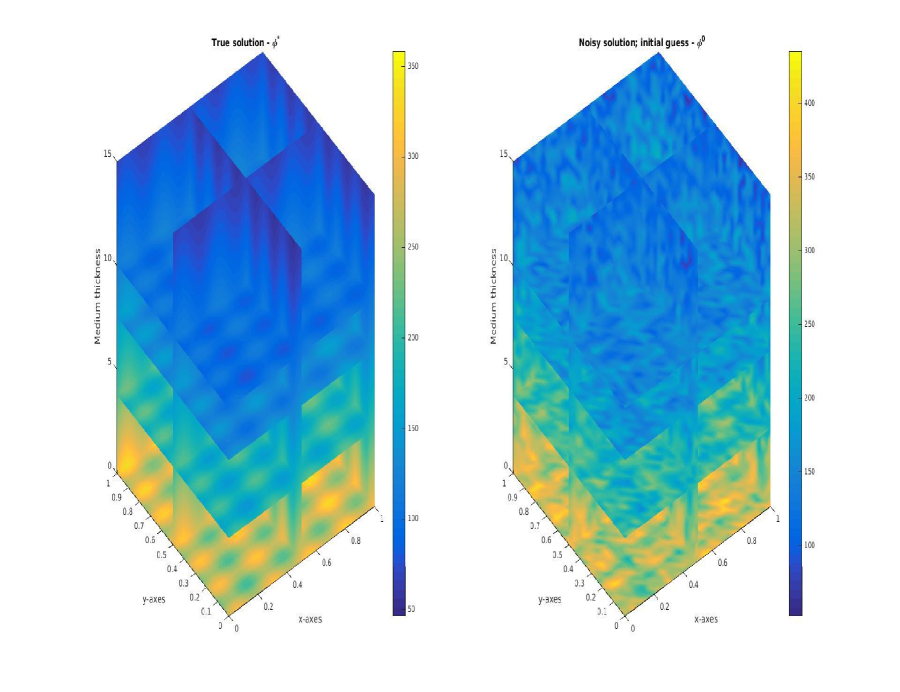
Figure 5: Simulated true and noisy solutions for the numerical experiments. The domain $\Omega$ has been discretized by $30\times 30\times 30$ points.

3.3 On the implementation of the forward operator

Thorough implementation and inversion of geodesic X-ray transform has been studied in [28]. Here, we focus on the linearized form of that regarding general implementation. In the computerized environment, we are only capable of implementing discretized integration which has been introduced in (3.2). In our implementation, this discretized integration is carried on according to nearest neighbor search, or closest point search, principle. To this end, discretization of each ray $\gamma$ is necessary. Owing to the parameter function $t(\epsilon)=\frac{\epsilon}{\sin(\tilde{\rho})},$ where $\epsilon\in[z_{s},h^{\infty}],$ we are able to discretize $\gamma,$ see (1.11). For one ray, this discretization is illustrated in Figure 6 whereby blue stars denote the mesh points of the signal path $\gamma$ and the red circles are for the nearest points to the corresponding mesh point of $\gamma.$ Discretized line integration is carried on along those red circles. The implemented integration procedure seeks the nearest point to the corresponding interior point of $\gamma$ on the horizontal layer. By the nearest point, we mean the closest grid point of the area of interest $\Omega$ to the interior point of the corresponding ray. This procedure can be described mathematically as such; For any index $k\in\{i,i+1\}$ where $i=1,\cdots,N-1,$ denote by $\vec{x}_{k}$ any grid point of our simulated area of interest $\Omega\subset\mathbb{R}^{3}.$ Interior point of any ray $\gamma_{[\mathbf{s},\vec{\theta}]}$ is denoted by $\vec{\gamma}_{l}$ for $l=1,\cdots,m,$ where $m$ is the number of the interior points. Then, we seek the closest point $\vec{x}_{k}\in\Omega$ to the interior point $\vec{\gamma}_{l}\in\gamma_{[\mathbf{s},\vec{\theta}]}$ according to the finite dimensional maximum norm by

$$d_{k}^{l}:=\min_{i}\{\|\vec{\gamma}_{l}-\vec{x}_{i}\|_{\infty},\|\vec{\gamma}_{l}-\vec{x}_{i+1}\|_{\infty}\}\mbox{, for }k\in\{i,i+1\}\mbox{ where }i=1,\cdots,N-1.$$ (3.18)

The pointwise density value at the corresponding point $\vec{x}_{k}\in\Omega\subset\mathbb{R}^{3}$ is $\varphi_{k}=\varphi(\vec{x}_{k}),$ for $k\in\{i,i+1\}$ where $i=1,\cdots,N-1.$ Eventually, the true measurement vector $f_{j}^{\dagger}$ for the corresponding ray is calculated by

$$[T\varphi]_{j}=\sum_{i=1}^{N}\varphi_{i}w_{i,j}=f_{j}^{\dagger}.$$ (3.19)

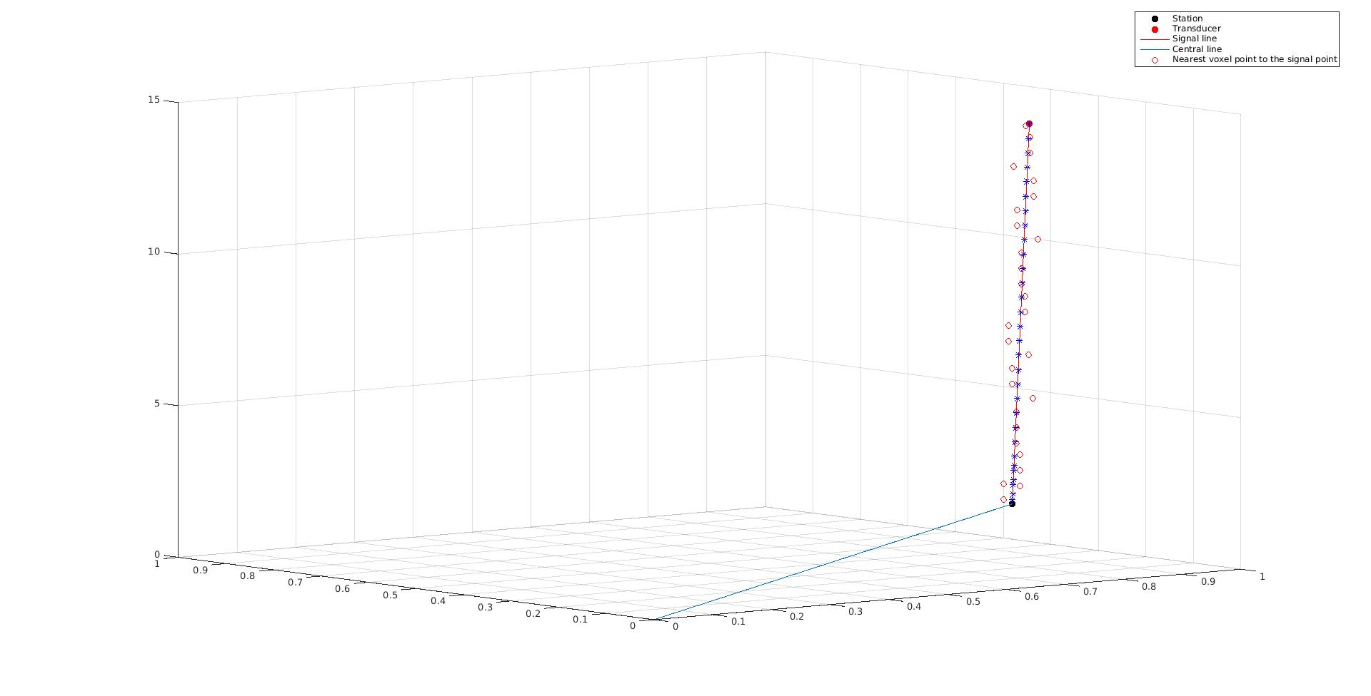
Figure 6: Demonstration for the line integration procedure.

4 Numerical Results and Review on the Algorithms

Since application of smooth TV is a new regularization strategy for this particular problem, it is expected to obtain some reasonable reconstruction. We will also realize usual facts in regularization theory. Firstly, this problem can also be interpreted as another sparse reconstruction. Therefore, measurement number (number of the signal) will impact on the convergence rate in the pre-image space. We will demonstrate this by the relative error value of the reconstruction. Secondly, as well known by the usual regularization theory for the inverse ill-posed problems [15], noise amount defined in the image space will also have impact on the convergence rate in the pre-image space. This latter case will also be demonstrated by visualizing the relative error value of the reconstruction.

4.1 Quasi-Newton Methods

Much of the technical and scientific details of this section can be found in [26, 32]. With a positive definite symmetric approximate Hessian $H_{\alpha}^{\nu}$ and properly chosen step-length parameter $\eta,$ one obtains the update $\varphi_{\alpha}^{\nu+1}$ by a quasi-Newton method as such,

$$\varphi_{\alpha}^{\nu+1}=\varphi_{\alpha}^{\nu}-\eta H_{\alpha}^{\nu}\nabla F_{\alpha}^{\nu}.$$ (4.1)

Here, $F_{\alpha}^{\nu}=F_{\alpha}(\varphi_{\alpha}^{\nu},f^{\delta}).$ Algorithms that provide the approximate solution $\varphi_{\alpha}^{\nu+1}$ are called gradient based algorithms, (cf. [2] and [3, Eq 2.1]).

4.2 Lagged Diffusivitiy Fixed Point Iteration - (LDFP)

The favourite regularization strategy of this work is TV regularization. Therefore, we would like to begin with one of the simplest algorithms to illustrate our regularized solution. LDFP, [44, 45], is also in the class of quasi-Newton search direction algorithm. Since the Fréchet differentiable functional $F_{\alpha}(\varphi,f^{\delta})$ is defined by

$$F_{\alpha}(\varphi,f^{\delta}):=\frac{1}{2}||{\mathcal{T}}\varphi-f^{\delta}||_{2}^{2}+\alpha\int_{\Omega}\sqrt{|\nabla\varphi(x)|^{2}+\beta}dx,$$

then LDFP is given by the following scheme,

$$\varphi_{\alpha}^{\nu+1} = \varphi_{\alpha}^{\nu}+({\mathcal{T}}^{\ast}{\mathcal{T}}+\alpha L(\varphi_{\alpha}^{\nu}))^{-1}\nabla F_{\alpha}(\varphi,f^{\delta})$$ (4.2)

$$= ({\mathcal{T}}^{\ast}{\mathcal{T}}+\alpha L(\varphi_{\alpha}^{\nu}))^{-1}{\mathcal{T}}^{\ast}f^{\delta}={\mathcal{R}}_{\alpha}(\varphi_{\alpha}^{\nu}),\hskip 5.69046pt\nu=0,1,\cdots,$$

where,

$$L(\varphi_{\alpha}^{\nu}):=-\nabla^{\ast}\cdot\left(\frac{\nabla}{(|\nabla\varphi_{\alpha}^{\nu}|^{2}+\beta)^{1/2}}\right).$$

Comparison between (4.2) and (4.1) yields that in the LDFP scheme the step-length $\eta=1,$ and the approximate Hessian is defined by

$$H_{\alpha}^{\nu}:={\mathcal{T}}^{\ast}{\mathcal{T}}+\alpha L(\varphi_{\alpha}^{\nu}).$$ (4.3)

Direct implementation of the scheme (4.2) would still be a costly iteration procedure since $L(\varphi)$ is highly nonlinear. Then, according to [44, Algorithm 8.2.3], the update $\varphi_{\alpha}^{\nu+1}$ is produced after the following linearization steps;

LDFP algorithm with smooth-TV penalty:

1. Compute $L^{\nu}:=L(\varphi_{\alpha}^{\nu})$ anisotropic Laplacian;

2. Compute $g^{\nu}:=\mathcal{T}^{\ast}(\mathcal{T}\varphi_{\alpha}^{\nu}-f^{\delta})+\alpha L^{\nu}\varphi_{\alpha}^{\nu}$ gradient step;

3. Compute $H_{\alpha}^{\nu}:=\mathcal{T}^{\ast}\mathcal{T}+\alpha L^{\nu}$ approximate Hessian;

4. Solve $H_{\alpha}^{\nu}s^{\nu+1}=-g^{\nu}$ quasi-Newton step;

5. Update $\varphi_{\alpha}^{\nu+1}=\varphi_{\alpha}^{\nu}+s^{\nu+1};$

In our experiments, we use usual CGNE for solving the inner system $H_{\alpha}^{\nu}s^{\nu}=g^{\nu},$ see [20]. In the Figure 7, we present the numerical results of LDFP algorithm per different number of the measurements. We run the algorithm only for $30$ iteration steps to understand its behaviour. Reconstructions that are the results of LDFP algorithm per different number of measurements are presented in Figure 8.

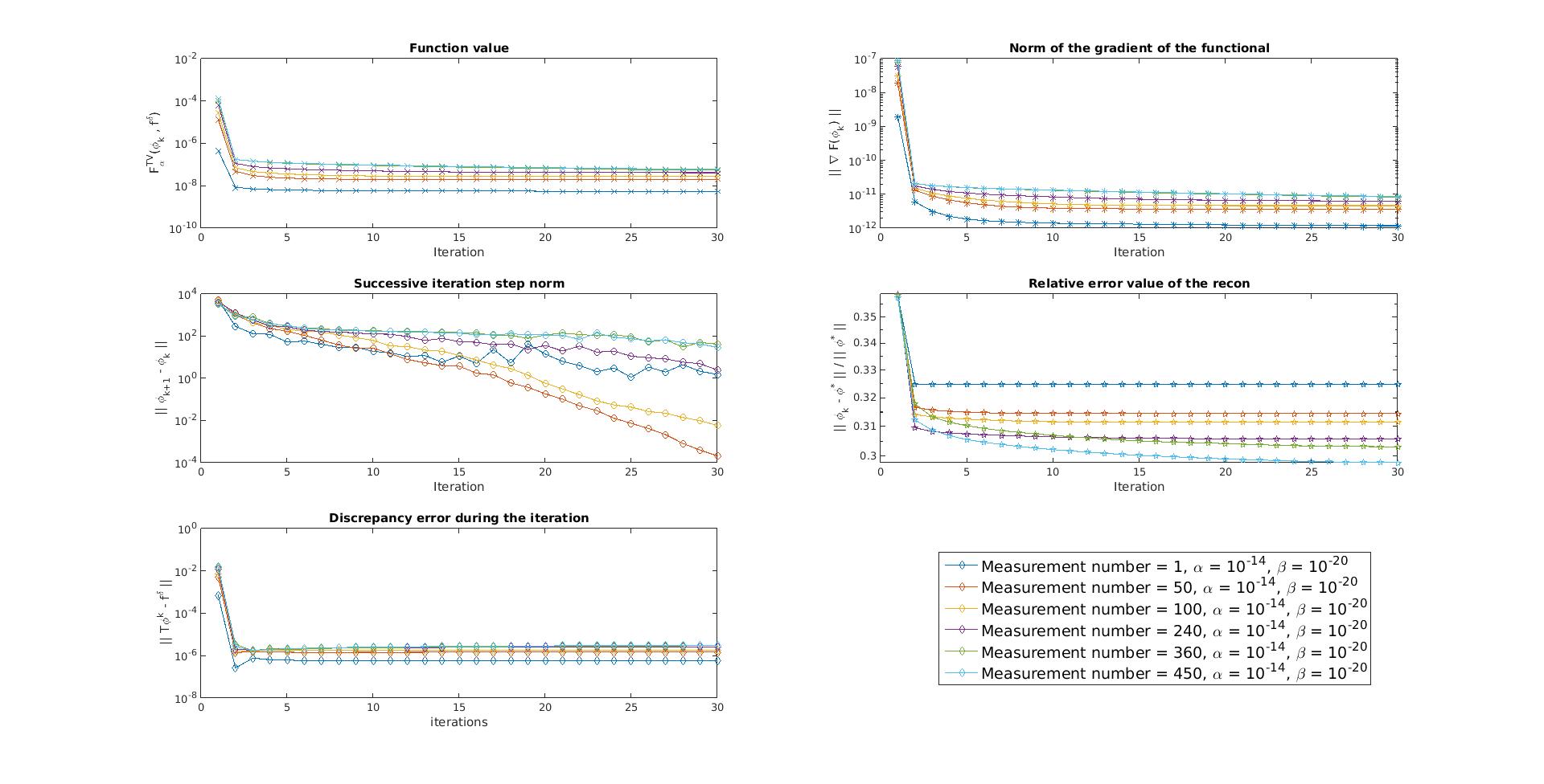
Figure 7: LDFP numerical convergence results per different number of the measurements, $\{1,50,100,240,360,450\}.$ Regularization parameter is chosen according to the stable behaviour of the discrepancy $||{\mathcal{T}}\varphi_{\alpha}^{\nu}-f^{\delta}||$ after each iteration step $\nu=1,2,3,\cdots.$

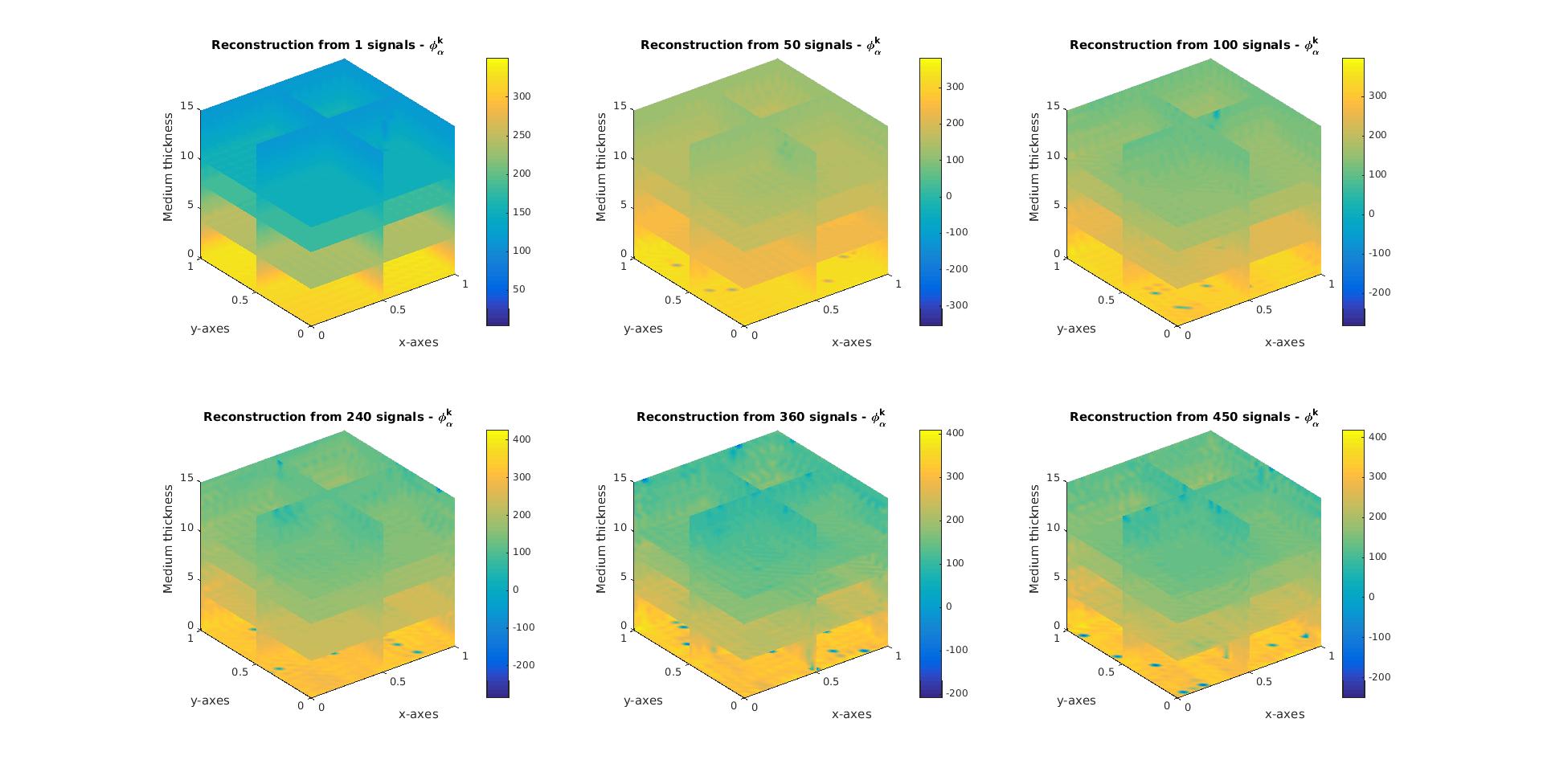
Figure 8: LDFP numerical reconstruction results per different number of the measurements, $\{1,50,100,240,360,450\}.$

4.3 Quasi-Newton method for large-scale problems

The quasi-Newton methods cannot be directly applicable to large optimization problems because their approximations to the Hessian or its inverse are usually dense. The storage and computational requirements grow in proportion to $N^{2},$ and become excessive for large $N.$ In order to overcome this difficulty, limited-memory quasi-Newton methods have been introduced, [26, 32]. Here, we particularly focus on limited memory BFGS (L-BFGS) algorithm.

By applying a quasi-Newton method, finding the optimum solution to the minimization problem (2.5), amounts to solving secant equation given by

$$B^{\nu+1}s_{\nu}=y_{\nu},$$ (4.4)

where

$$s_{\nu}=\varphi_{\alpha}^{\nu+1}-\varphi_{\alpha}^{\nu},\mbox{ }y_{\nu}=\nabla F_{\alpha}^{\nu+1}-\nabla F_{\alpha}^{\nu}.$$ (4.5)

Here, $F_{\alpha}^{\nu}=F_{\alpha}(\varphi_{\alpha}^{\nu},f^{\delta}).$ In (4.4), the matrix $B^{\nu+1}$ is a positive definite symmetric approximation to the true Hessian of the cost functional $F_{\alpha}.$

$$\varphi_{\alpha}^{\nu+1}=\varphi_{\alpha}^{\nu}-\eta^{\nu}H^{\nu}\nabla F_{\alpha}^{\nu}.$$ (4.6)

Here the aproximate Hessian $H^{\nu}$ is updated by ,

$$H^{\nu+1}=V_{\nu}^{T}H^{\nu}V_{\nu}+\rho_{\nu}s_{\nu}s_{\nu}^{T}$$ (4.7)

with,

$$\rho_{\nu}=\frac{1}{y_{\nu}^{T}s_{\nu}},\mbox{ }V_{\nu}=I-\rho_{\nu}y_{\nu}s_{\nu}^{T}.$$ (4.8)

4.4 L-BFGS with trust region

Robustness of L-BFGS algorithm is provided by trust regions, [13, p. 232][26, p. 91]. The trust region is the set of all points, [11],

$${\mathcal{B}}^{\nu}:=\{\varphi_{\alpha}^{\nu}\mbox{ }|\mbox{ }||\varphi-\varphi_{\alpha}^{\nu}||\leq\Delta^{\nu}\}.$$

Trust-region subproblem with trust-region radius $\Delta^{\nu}$ has been described well in [26, p. 94].

We provide the optimized solution for our problem (2.5) from trust region L-BFGS algorithm by employing a novel reverse-communication large-scale nonlinear optimization software SAMSARA, [25], [26, Subsection 5.2.3]. We demonstrate different solution per different measurement number, $\{1,50,100,240,360,450\},$ in the figures 9, 10, 11, 12. It is observed better and more stable convergence rate in the pre-image space with the more measurement number in the image space. Furthermore, the figures 13 and 14 demonstrate convergence in the pre-image/image spaces with varying amount of noise, $\delta\in\{20\%,10\%,5\%,2\%,0.1\%,0.005\%,0.001\%\}.$ As a common expectation from an inverse ill-posed problem, the less amount of noise in the image space provides better and stable convergence rates in the pre-image space.

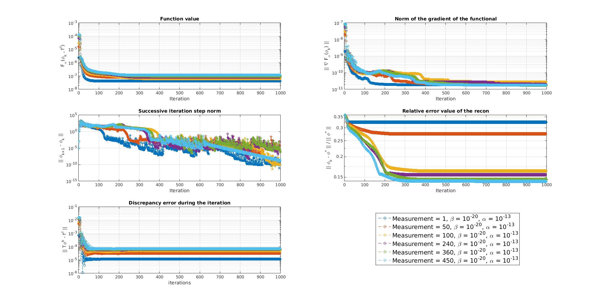
Figure 9: SAMSARA with TV gradient step numerical results per measurement. We have conducted our experiment in the software SAMSARA for the measurement number $\{1,50,100,240,360,450\}.$

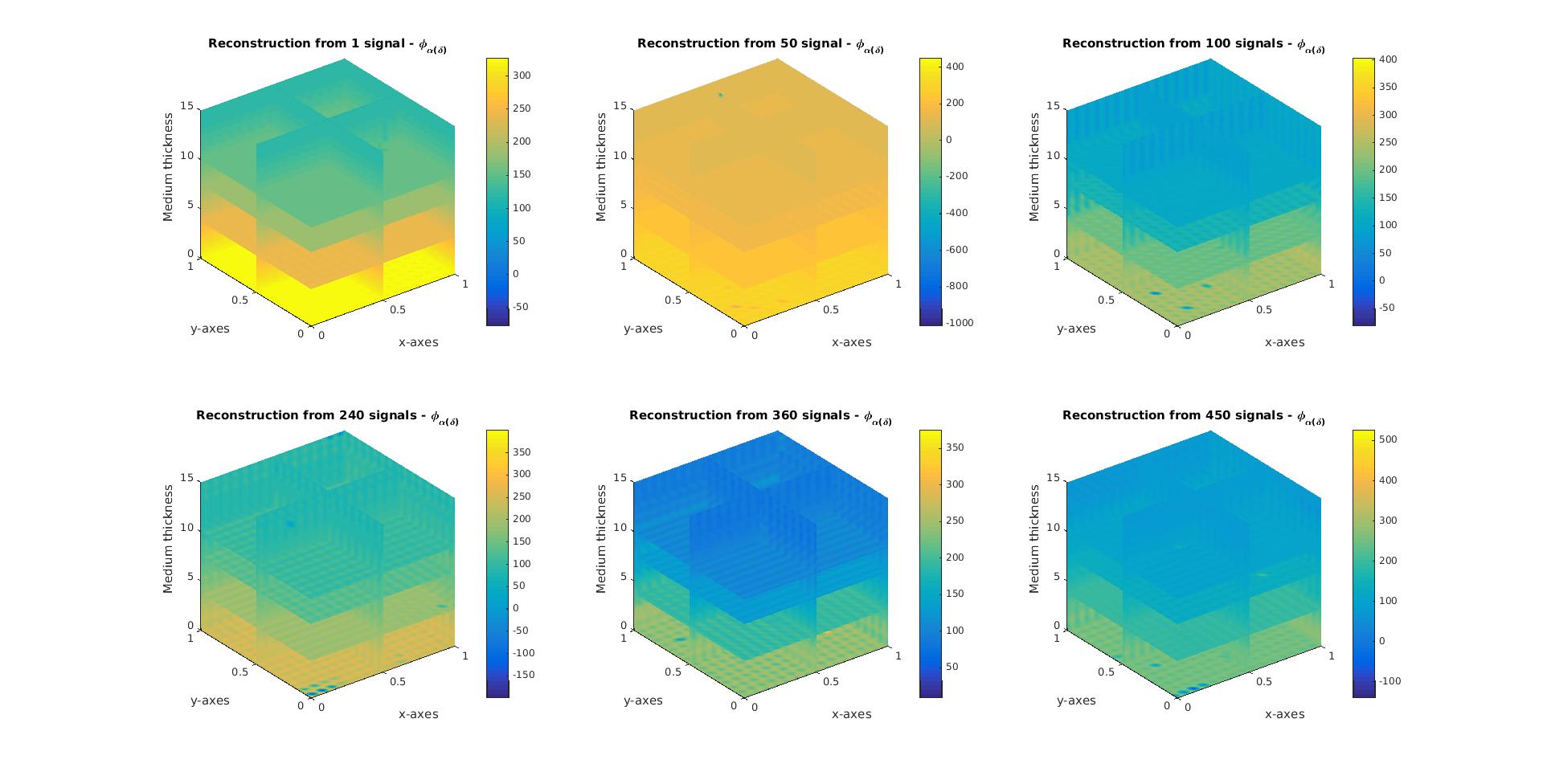
Figure 10: SAMSARA with TV gradient step numerical reconstruction results per measurement $\{1,50,100,240,360,450\}.$ Fixed regularization parameter $\alpha=10^{-13}$ has been determined according to the behaviour in the discrepancy.

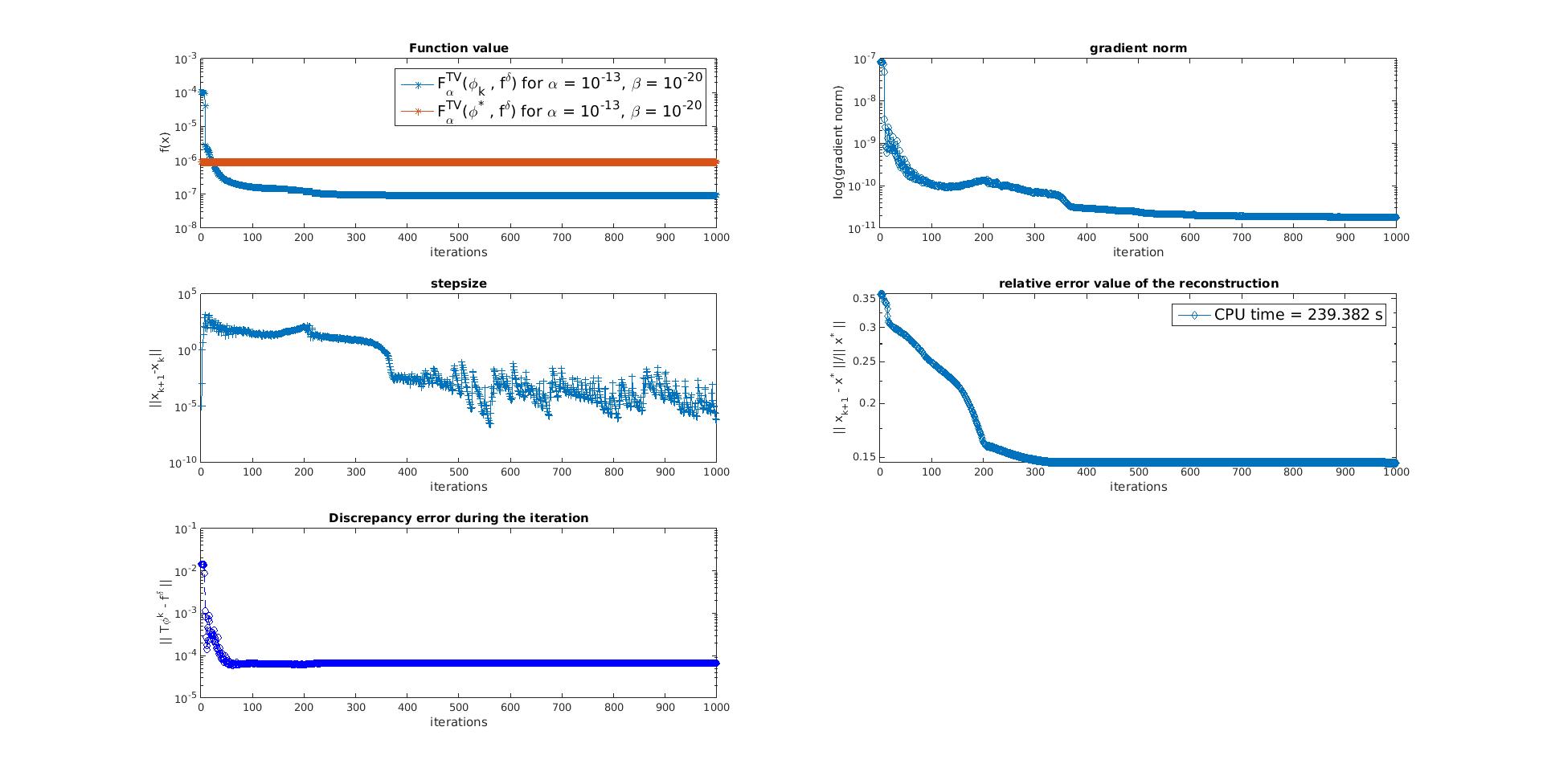
Figure 11: SAMSARA numerical convergence from 360 signals.

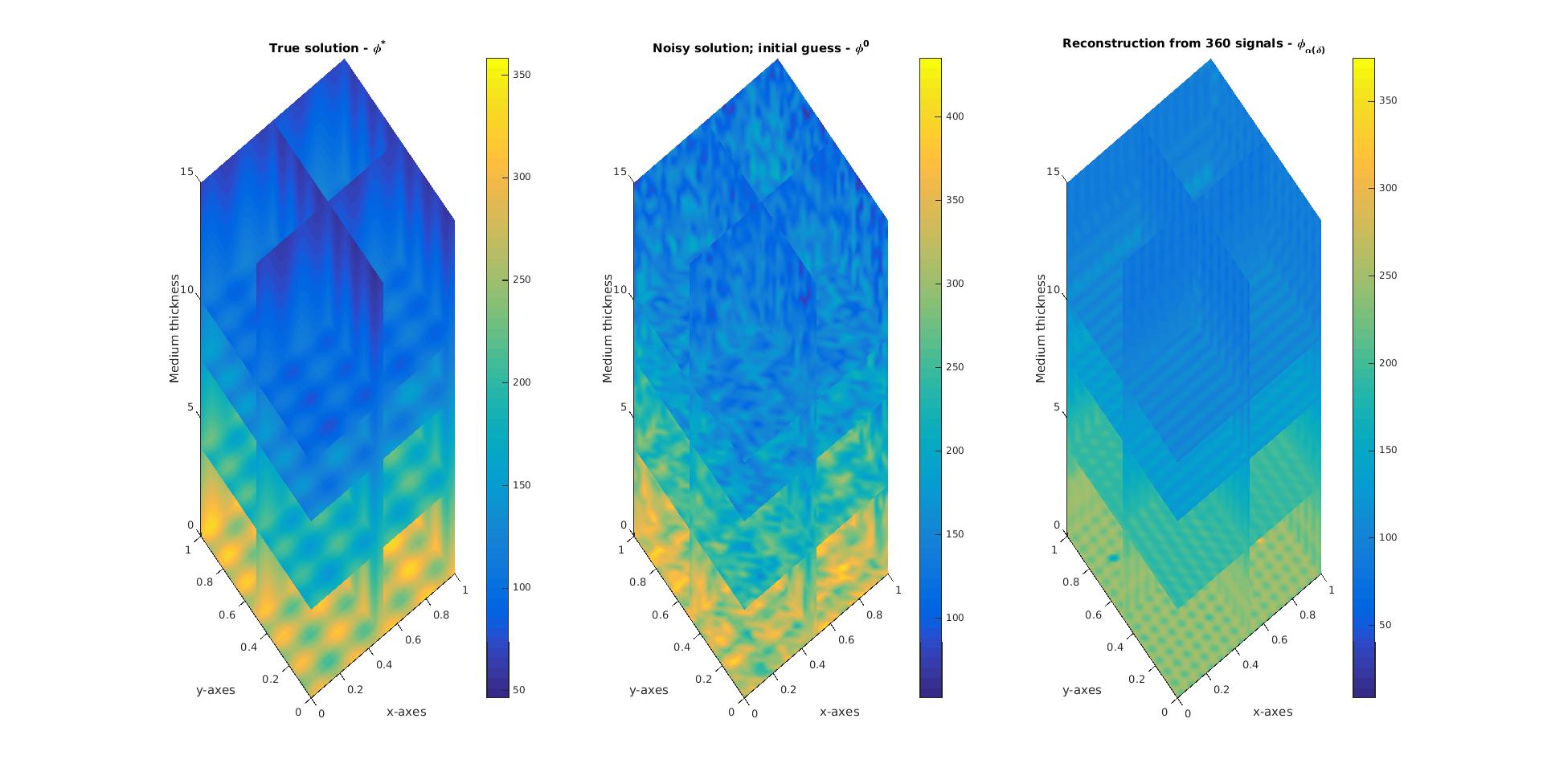
Figure 12: SAMSARA numerical reconstruction from 360 signals.

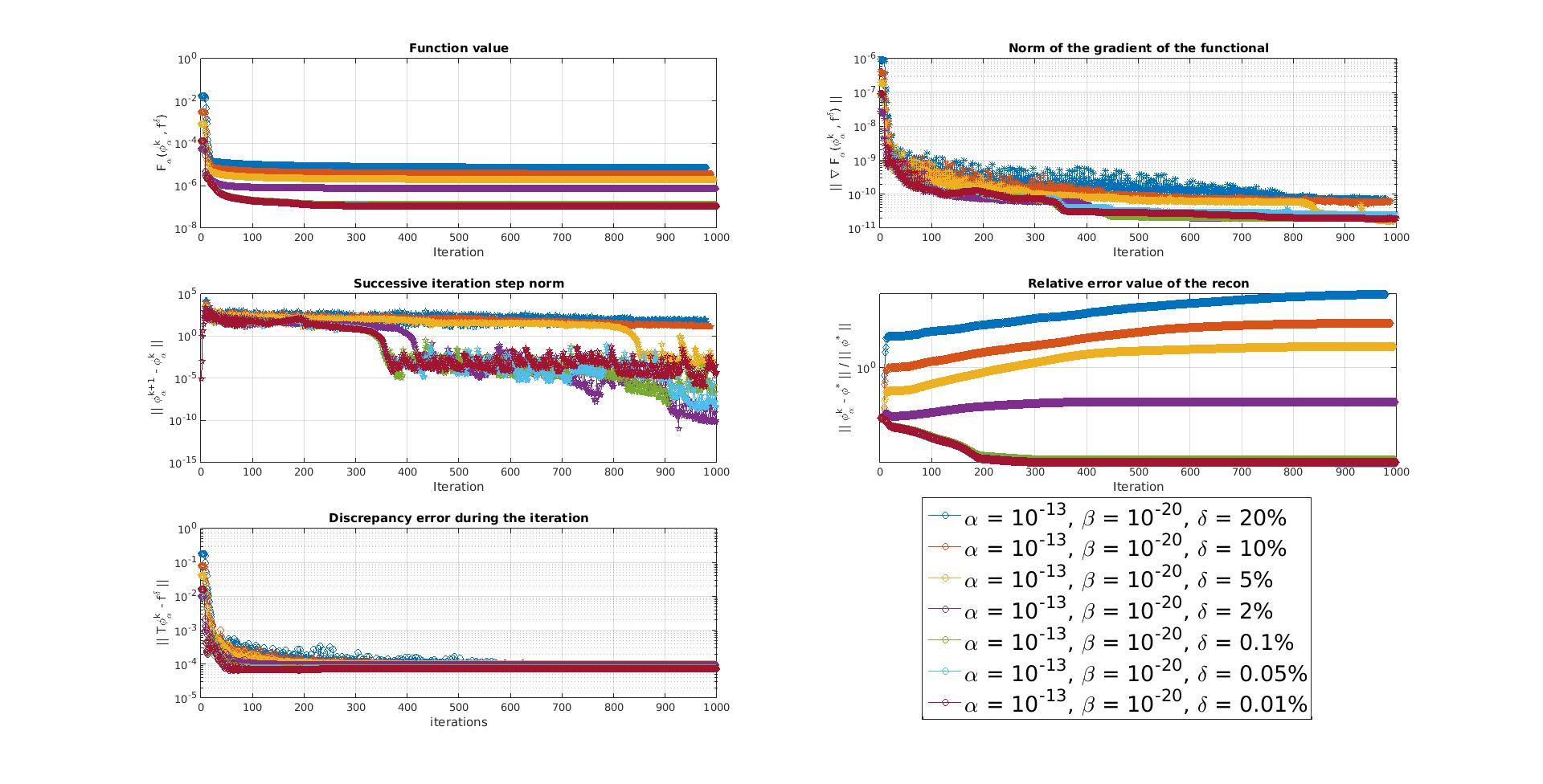
Figure 13: SAMSARA with TV gradient step convergence analysis per different noise amount $\{20\%,10\%,5\%,2\%,0.1\%,0.005\%,0.001\%\}.$ Convergence in the pre-image space begins with $\delta\leq 2\%.$

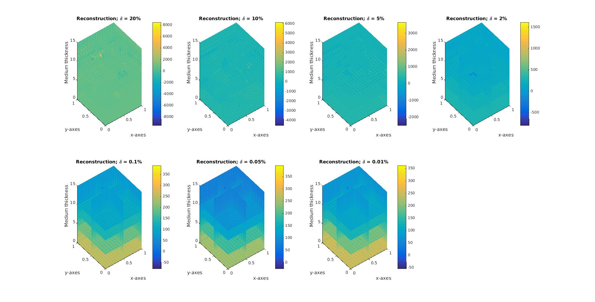
Figure 14: SAMSARA with TV gradient step different reconstruction per different noise amount. Corresponding numerical convergence analysis has been provided in Figure 13.

4.5 Further reconstructions by L-BFGS with quadratic penalty Term

As a concrete demonstration for the effectiveness of TV type reconstruction, we also seek approximate minimizer for the classical Tikhonov type functional with the quadratic term below,

$$F_{\alpha}(\varphi,f^{\delta})=\frac{1}{2}||{\mathcal{T}}\varphi-f^{\delta}||_{{\mathcal{L}}^{2}({\mathcal{Z}})}^{2}+\alpha\frac{1}{2}||\varphi-\varphi^{(0)}||_{{\mathcal{L}}^{2}(\Omega)}^{2},$$ (4.9)

with some given initial guess $\varphi^{0}.$ Here, we only present numerical results produced by SAMSARA, [25], with quadratic Tikhonov type objective functional. Then the gradient step of the objective functional in (4.9) to be implemented is

$$\nabla F_{\alpha}(\varphi,f^{\delta})={\mathcal{T}}^{\ast}({\mathcal{T}}\varphi-f^{\delta})+\alpha(\varphi-\varphi^{(0)}).$$ (4.10)

We again run our tests with different number of measurements $\{1,50,100,240,360,450\}$ with sufficiently small amount of noise $\delta.$ Numerical convergence for each reconstruction is presented in Figure 15. Each reconstruction is presented in Figure 16.

Figure 15: SAMSARA results from quadratic Tikhonov gradient step numerical results per measurement. We have conducted our experiment in the software SAMSARA for the measurement number $\{1,50,100,240,360,450\}.$ Fixed regularization parameter $\alpha=10^{-15}$ has been determined according to the behaviour in the discrepancy after each iteration step $\nu=1,2,\cdots$.

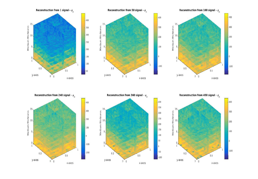
Figure 16: SAMSARA result from quadratic Tikhonov gradient step numerical reconstruction results per measurement $\{1,50,100,240,360,450\}$ for the fixed regularization parameter $\alpha=10^{-15}$

5 Benchmark: LDFP vs SAMSARA With Smoothed-TV Penalty

A CPU time based benchmark test between SAMSARA and LDFP both associated with the smoothed-TV gradient step has been conducted, see the figures 17, 18 and 19.

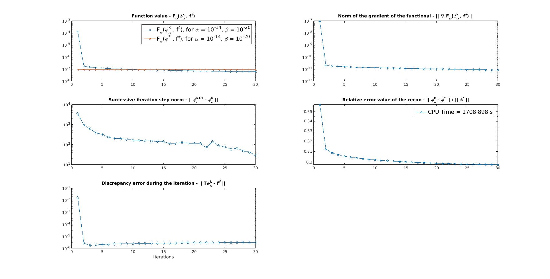
Figure 17: LDFP numerics from 450 measurements.

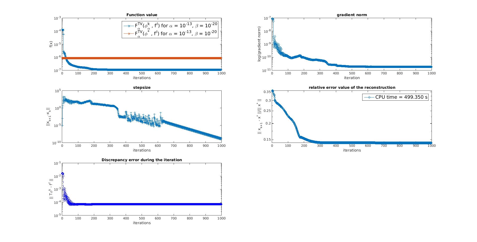
Figure 18: SAMSARA with smoothed-TV gradient step numerics from 450 measurements.

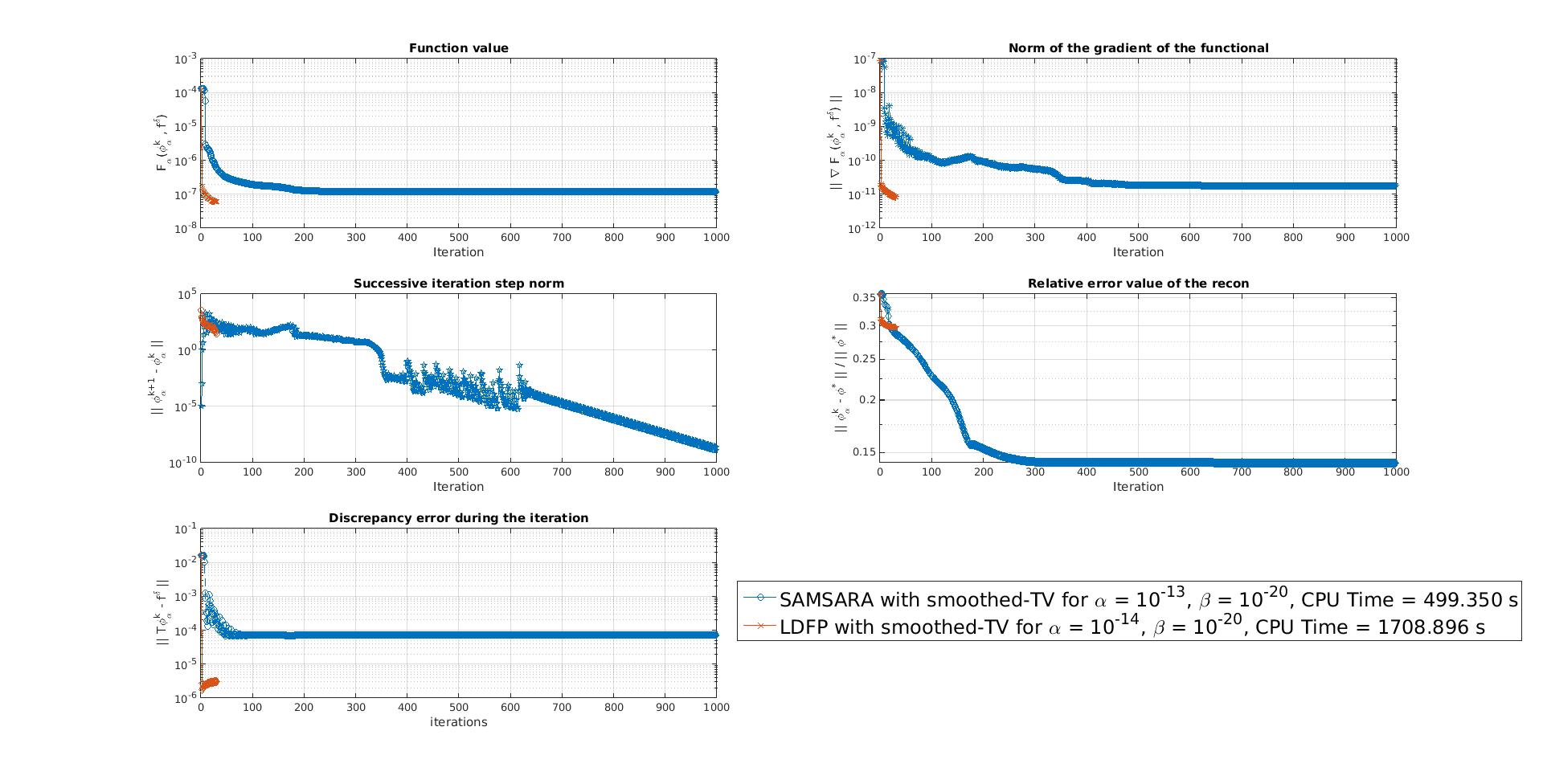
Figure 19: Benchmark: SAMSARA and LDFP numerics from 450 measurements. Recall from the figures 17 and 18 that LDFP got executed only for 30 iteration steps whereas SAMSARA 1000 iteration steps. Comparing the CPU times for each tests, it would take SAMSARA only 14.9805 seconds to iterate 30 times. In other words, SAMSARA works 33 times faster than usual LDFP algorithm with smoothed-TV gradient step.

6 Conclusion and Future Prospects

Although this is a time dependent inverse problem, we have considered that we receive certain number of measurements at a fixed time instant. However, we still aim to observe expected degradation in the convergence rates in the pre-image space based on different number of the measurements and the noise amount. In conclusion, more observations in the image space imply better convergence rate in the pre-image space. As expected from any inverse ill-posed problems, it also has been observed that less amount of noise in the image space implies better convergence rate in the pre-image space.

Due to the physical property of the targeted medium, the actual task is reconstruction of some non-negative function $\varphi:\Omega\subset\mathbb{R}^{3}\rightarrow\mathbb{R}_{+}.$ However, we have formulated an unconstrained, smooth, convex minimization problem (2.5). When the non-negativity constraint is taken into account, a new minimization problem must be stated as such,

$$\varphi_{\alpha}^{\delta}\in{\rm arg\,min}_{\varphi\in{\mathcal{V}}}\left\{\frac{1}{2}||{\mathcal{T}}\varphi-f^{\delta}||_{{\mathcal{H}}}^{2}+\alpha J(\varphi)\right\},$$ (6.1)

$$\varphi(x)\geq 0,\mbox{ for }x\in\Omega\subset\Omega_{o},$$ (6.2)

where $J:{\mathcal{V}}\rightarrow\mathbb{R}_{+}$ is some appropriately chosen penalty term.

7 Acknowledgement

This work was supported by German Weather Service (Deutscher Wetterdienst - DWD) project ” GPS-Tomography for atmospheric data assimilation” and SFB-755 by University of Göttingen. Author is thankful to D. Russell Luke for the access to the software SAMSARA for the correct implementation and the design of the three dimensional total variation penalty term. Furthermore, author also wishes to thank Thorsten Hohage for the fruitful discussions over the modelling of the tomography problem.

References

References

- [1] R. Acar and C. R. Vogel. Analysis of bounded variation penalty methods for ill-posed problems, Inverse Problems, 10, 6, 1217 - 1229, 1994.
- [2] A. Beck and M. Teboulle. Fast gradient-based algorithms for constrained total variation image denoising and deblurring problems, IEEE Trans. Image Process., 18, no. 11, 2419-2434, 2009.
- [3] A. Beck and M. Teboulle. A Fast Iterative Shrinkage-Thresholding Algorithm for Linear Inverse Problems, SIAM J. Imaging Sciences, 2, 1, 183-202, 2009.
- [4] M. Bender, G. Dick, M. Ge, Z. Deng, J. Wickert, H. G. Kahle, A. Raabe, G. Tetzlaff. Development of a GNSS water vapour tomography system using algebraic reconstruction technique, ADV SPACE RES, 47(10):1704-1720, 2011.
- [5] M. Benning, L. Gladden, D. Holland, C.-B. Schönlieb and T. Valkonen. Phase reconstruction from velocity-encoded MRI measurements - a survey of sparsity-promoting variational approaches. Journal of Magnetic Resonance, 238, 26 - 43, 2014.
- [6] A. Chambolle, P.L. Lions. Image recovery via total variation minimization and related problems, Numer. Math. 76, 167 - 188, 1997.
- [7] T. F. Chan and P. Mulet. On the convergence of the lagged diffusivity fixed point method in total variation image restoration, SIAM J. Numer. Anal., 36, 2, 354-367, 1999.
- [8] T. Chan, G. Golub and P. Mulet. A nonlinear primal-dual method for total variation-baes image restoration, SIAM J. Sci. Comp, 20, 1964-1977, 1999.
- [9] P. G. Ciarlet. Linear and nonlinear functional analysis with applications, Society for Industrial and Applied Mathematics, Philadelphia, PA, 2013.
- [10] D. Colton and R. Kress. Inverse Acoustic and Electromagnetic Scattering Theory, Springer Verlag Series in Applied Mathematics Vol. 93, Third Edition 2013.
- [11] A. R. Conn, N. I. M. Gould, P. L. Toint. Trust-Region Methods. MPS-SIAM Series on Optimization, 2000.
- [12] L. Debnath and P.Mikusiński, Introduction to Hilbert spaces with applications, 3rd Editoin, Elsevier Academic Press, 2005.
- [13] J. E. Dennis and R. Schnabel. Numerical Methods for Unconstrained Optimization and Nonlinear Equations. Prentice Hall, 1983.
- [14] D. Dobson and O. Scherzer. Analysis of regularized total variation penalty methods for denoising, Inverse Problems, 12, 5, 601 - 617, 1996.
- [15] H. W. Engl, M. Hanke and A. Neubauer. Regularization of inverse problems. Math. Appl., 375. Kluwer Academic Publishers Group, Dordrecht, 1996.
- [16] L. C. Evans. Partial differential equations, Graduate Studies in Mathematics, 19. American Mathematical Society, Providence, RI, 1998.
- [17] C. W. Grötsch. Inverse Problems in the Mathematical Sciences. Vieweg, 1993.
- [18] C. W. Grötsch. Integral equations of the first kind, inverse problems and regularization: a crash course. J. Phys.: Conf. Ser., 73, 012001, 2007.
- [19] C. Hamaker, K. T. Smith, D. C. Solmon, S. L. Wagner. The divergent beam x-ray transform, Rocky Mountain J. Math., 10, No.1, 253 - 283, 1980.
- [20] M. Hanke. Conjugate gradient type methods for ill-posed problems. Pitman Research Notes in Mathematics Series, 327. Longman Scientific & Technical, Harlow, 1995.
- [21] V. Isakov. Inverse problems for partial differential equations. Second edition. Applied Mathematical Sciences, 127. Springer, New York, 2006.
- [22] H. Kekkonen, M. Lassas and S. Siltanen. Analysis of regularized inversion of data corrupted by white Gaussian noise. Inverse Problems, 30, 045009, 18pp, 2014.
- [23] A. Kirsch. An Introduction to the Mathematical Theory of Inverse Problems. Second edition. Applied Mathematical Sciences, 120. Springer, New York, 2011.
- [24] F. Kleijer. Troposphere Modeling and Filtering for Precise GPS, Leveling Mathematical Geodesy and Positioning. Dissertation, ISBN: 90-804147-3-5, NUGI: 816, 2004.
- [25] R.Luke. SAMSARA, a reverse communication optimization toolbox for MATLAB, http://num.math.uni-goettingen.de/~r.luke/publications/SAMSARA_MATLAB.tar.gz
- [26] D. R. Luke. Analysis of optical wavefront reconstruction and deconvolution in adaptive optics. Dissertation, Department of Applied Mathematics, University of Washington, June 2001.
- [27] P. Miidla, K. Rannat P. Uba. Tomographic approach for tropospheric water vapor detection, Comput. Methods. Appl. Math., 8(3), 263-278, 2008.
- [28] F. Monard. Numerical Implementation of Geodesic X-Ray Transforms and Their Inversion. SIAM J. IMAGING SCIENCES, 7, 2, 1335 - 1357, 2014.
- [29] F. Natterer. The mathematics of computerized tomography, SIAM, Classics Appl. Math., 32, 2001.
- [30] F. Natterer. X-ray Tomography. Inverse Problems and Imaging, Springer, Berlin, 17 - 34, 2008.
- [31] F. Natterer and F. Wübbeling. Mathematical methods in image reconstruction, SIAM Monogr. Math. Model. Comput., 05, 2001.
- [32] J. Nocedal and S. J. Wright. Numerical Optimization. Springer Series in Operations Research. Springer-Verlag, New York, xxii+636 pp, 1999.
- [33] G. Ólafsson, E. T. Quinto. The Radon transform, inverse problems and tomography, Proceedings of Symposia in Applied Mathematics, Volume 63, American Mathematical Society Short Course, January 3-4, 2005, Atlanta, Georgia, 2006.
- [34] S. S. Orlov. Theory of three dimensional reconstruction II: The recovery operator. Soviet Phys. Crystallogr., 20, 429 - 433, 1976.
- [35] D. Perler, A. Geiger and F. Hurter. 4D GPS water vapor tomography: new parameterized approaches. J. Geod., 85, 539-550, 2011.
- [36] J. Radon. Über die Bestimmung von Funktionnen durch ihre Integralwerte längs gewisser Mannigfaltikeiten. Ber. Verh. Sachs. Akad. Wiss. Leipzig-Math.-Natur. Kl., 69, 262 - 277, 1917.
- [37] L. I. Rudin, S. J. Osher, E. Fatemi. Nonlinear total variation based noise removal algorithms, Physica D, 60, 259-268, 1992.
- [38] W. Rudin. Principles of Mathematical Analysis. Third edition, International Series in Pure and Applied Mathematics. McGraw-Hill Book Co., New York-Auckland-Düsseldorf, 1976.
- [39] O. Scherzer, M. Grasmair, H. Grossauer, M. Haltmeier F. Lenzen. Variational Methods in Imaging. Applied Mathematical Sciences, 167, Springer, New York, 2009.
- [40] U. Schröder and T. Schuster. An Iterative Method to Reconstruct the Refractive Index of a Medium From Time-of-Flight Measurements. arXiv:1510.06899v1 , 2015.
- [41] D. F. Shanno and K. Phua. Matrix conditioning and nonlinear optimization. Math. Prog., 14, 149 - 160, 1978.
- [42] K. T. Smith, D. C. Solmon, S. L. Wagner, C. Hamaker. Mathematical aspects of divergent beam radiography, Proc. Natl. Acad. Sci. USA, 75, No. 5, 2055 - 2058, 1978.
- [43] C. R. Vogel. A limited memory BFGS method for an inverse problem in atmospheric imaging. Methods and Applications of Inversion, Lecture Notes in Earth Sciences, 92, 292-304, 2000.
- [44] C. R. Vogel. Computational methods for inverse problems, Frontiers Appl. Math. 23, 2002.
- [45] C. R. Vogel , M. E. Oman. Iterative methods for total variation denoising, SIAM J. SCI. COMPUT., Vol. 17, No. 1, 227-238, 1996.
- [46] F. Zus, M. Bender, Z. Deng, G. Dick, S. Heise, M. Shang-Guan, J. Wickert, A methodology to compute GPS slant total delays in a numerical weather model, Radio Science, 2012, vol. 47, RS2018.