Numerical reconstruction of pulsatile blood flow from 4D computer tomography angiography data
Abstract
We present a novel numerical algorithm developed to reconstuct pulsatile blood flow from ECG-gated CT angiography data. A block-based optimization method was constructed to solve the inverse problem corresponding to the Riccati-type ordinary differential equation that can be deduced from conservation principles and Hooke’s law. Local flow rate for patients was computed in cm long aorta segments that are located cm below the heart. The wave form of the local flow rate curves seems to be realistic. Our approach is suitable for estimating characteristics of pulsatile blood flow in aorta based on ECG gated CT scan thereby contributing to more accurate description of several cardiovascular lesions. 222Submitted to Computers and Mathematics With Applications, 2015. (lovas@math.bme.hu)
Keywords: biofluid mechanics; pulsatile flow ; inverse problem ; periodic Ricatti equation
MSC2010 numbers: 65M32; 65K10; 76Z05; 92C10; 92C50
1Budapest University of Technology and Economics, Department of Analysis, Building H, Egry József str. 1, Budapest, Hungary 1111
2Budapest University of Technology and Economics, Department of Structural Mechanics, Building K, Műegyetem rkp. 3, Budapest, Hungary 1111
3Budapest University of Technology and Economics, Department of Geometry, Building H, Egry József str. 1, Budapest, Hungary 1111
4Semmelweis University, Heart and Vascular Center, Department of Vascular Surgery, Városmajor str. 68, Budapest, Hungary 1122
1 Introduction
Pulsatile flow in blood vessels has been studied for more than 300 years. Leonard Euler initiated the theory of pressure wave propagation in the vascular system in 1775. The first modern mathematical model of pulsatile flow in blood vessels was developed by Diederik Johannes Korteweg and Horace Lamb. Hitherto, numerous attempts have been made to study blood flow in the vascular system. Yunlong Huo and Ghassan S. Kassab have published a Womersley-type mathematical model to analyze pulsatile blood flow in the entire coronary arterial tree [1]. Mostly stenosed geomeries were investigated owing to their connection to vascular diseases such as arteriosclerosis which may lead to heart attack and stroke [2]. Mir Golam Rabby et al. have investigated numerically the effects of non-Newtonian modeling on unsteady periodic flows in a two-dimensional pipe with idealized stenoses [3]. In the above mentioned studies, motions of the vessel wall were not taken into consideration.
ECG-gated computer tomography along with an image segmentation algorithm based on Active Contour Model [4] enables us to measure the local cross sectional area of the vessel as a function of time and the position of the considered cross section along the vessel’s axis. The main objective of the present work is to develop a numerical procedure to compute volumetric flow rate of blood through the local cross sections of the vessel from the local cross sectional area. We assume that there exist a short segment of the vessel where it is thin and elastic. Furthermore, the change in the local cross sectional area must be caused by the change in blood pressure only, and gravitation has no effect on the fluid because the patient is lying during the medical examination. By applying the one-dimensional Euler momentum equation, equation of continuity and Hooke’s law, we deduced a Riccati-type ODE for volumetric flow rate at the beginnig of the considered vessel segment closer to the heart. The only periodic solution with positive integral was accepted as physically admissible. Existence of such a solution can be tested numerically. However, the Riccati-type ODE contains an extra scalar parameter and can be solved just for fixed parameter values. To find the volumetric flow rate a block-based optimization method was implemented.
2 Material and methods
2.1 ECG-gated CT angiography
Imaging of a pulsatile organ is a highly demanding application for any cross sectional imaging modality. Computed tomography (CT) imaging of the heart became widely available with the introduction of multi-detector CT (MDCT) scanners with four-slice detector arrays and 500 ms minimum rotation time [5]. Still images of the moving heart was generated using retrospective ECG-gating: slow table motion during spiral scanning and simultaneous acquisition of the slices and the digital ECG trace provided oversampling of scan projections [5]. After the exposure, slices recorded in the same phase of the ECG trace are matched to generate a 3D dataset of the volume of interest, representing either systole or diastole. A drawback of this method is the higher radiation dose compared to the normal non-oversampled spiral acquisition [6]. An important advantage is the possibility to reconstruct multiphasic datasets of the same volume, resulting in motion images of the same slices. This allows us the functional analysis of the moving organs such as the heart or the large vessels. Recent advances in CT technology ( detector rows, ms minimum rotation time) allow for rapid ECG-gated CTA of the whole aorta during a single breath-hold.
Imaging of the aorta was performed in patients ( men, mean age years) with a -slice MDCT (Philips Brilliance iCT, Koninklijke Philips N.V., Best, The Netherlands) using a retrospectively ECG-gated protocol tailored for the imaging of the aorta. Investigations were performed on images readily available from patients with suspected aortic disease. Low-dose (tube voltage: kV) native scan was followed by a retrospective ECG-gated CT angiography of the whole aorta ( kV) with a reduced field of view to maximize spatial resolution. Nonionic contrast agent was injected into an antecubital vein at a flow rate of ml/s using a power injector. Images were reconstructed using a sharp convolution kernel and iterative reconstruction algorithm (iDose4, Koninklijke Philips N.V., Best, The Netherlands) with a slice thickness of mm and an increment of mm. Multiphase images were reconstructed corresponding every 10% of the R-R cycle resulting in ten series of images for each patient. Patients gave written informed consent before CT examination was performed. Experimental protocol and informed consent was approved by the Regional Ethical Committee of Semmelweis University ().
2.2 Image segmentation
The first problem which we have to solve in order to compute cross sectional area of the blood vessel is to locate it in the dicom image. This can be carried out by some sort of image segmentation algorithm. In our case, Actice Contour Model (ACM) was applied to perform segmentation. The first version of ACM was published by Michael Kass, Andrew Witkin and Demetri Terzopoulos [4] at the end of the 80s.
Active contours are energy minimizing splines in 2D which they are commonly referred to as snakes. It is possible to generalize the algorithm to higher dimensions using energy minimizing surfaces but the corresponding numerical method is usually not stable because a surface might intersect itself or change its topology. For that reason, an algorithm based on a sequential two-dimensional balloon snake model was applied to each phase which means that the final position of the moving snake on a slice was implemented as initial condition on the next one. As the result of the segmentation process, we get the coordinates of the vessel’s internal wall for each slice perpendicular to axis in the region of interest and for all phases in time. For more information about the Active Contours we refer the reader to [7] and [8].
To mitigate the spatial measurement error, we fitted a bicubic smoothing spline to the point cloud resulting from the active contour method in each time step. This way the increase of temporal resolution also became possible exploiting the affine covariance of B–splines and ensuring the periodic movement of the control points by trigonometric approximation using the first 3 harmonics of the heart rate [9]. The cross-sectional area is defined as the area of the section perpendicular to the center line of the fitted surface.
2.3 Governing Equations
To make our exposition self-contained we present some laws of continuum mechanics, these are the conservation laws for mass and momentum. In addition, empirical constitutive laws are needed to relate certain unknown variables such as relations between stress and strain.
Let us examine the pulsating flow of blood in an artery assuming that the wall is thin and elastic. Owing to the pressure gradient the artery wall deforms and the elastic restoring force of the wall makes it possible for waves to propagate and so it maintains a pulsating motion of the artery. The artery radius varies in time along the artery. Let the local cross sectional area be and the averaged flow velocity are periodic in the first argument with period where denotes the period of the cardiac cycle. We define the volume flow rate as . Assuming that blood is homogeneous and incompressible we obtain from the law for conversation of mass that
| (1) |
Additionally the law for conservation of momentum can be written as follows:
| (2) |
We use Hooke’s law to relate stress and strain rates. Let be the vessel wall thickness, assumed to be much smaller than the vessel radius, and Young’s modulus will be denoted by . The change in tube radius must be caused by the blood pressure. The elastic strain due to the lengthening of the circumference is . The change is elastic force must be balanced by the changing in pressure force , which implies
From this we obtain the following:
| (3) |
3 Calculation
3.1 Periodic Riccati equation
Let us consider a nonbranching cylindral blood vessel segment of length where equations (1), (2) and (3) are satisfied. If we substitute (3) into (2) we have
| (4) |
where is assumed to be constant during the cardiac cycle.
If we multiply the left-hand side of (4) by , using and integrating by parts we obtain
| (5) |
By applying (1), the volumetric flow rate can be written as
| (6) |
where and
From this we obtain the following Riccati-type ordinary differential equation
| (7) |
where coefficients are periodic with period and can be written as follows:
| (8) | ||||
| (9) | ||||
| (10) |
3.2 Periodic solutions
Physically admissible solutions
Assume that corresponds to the beginnig of the considered vessel segment closer to the heart.
Definition 1
A solution of (7) is said to be physically admissible if it satisfies the following conditions:
-
i.
is a periodic function with period ,
-
ii.
.
It is well known that the general solution of a scalar Riccati equation can be obtained by quadrature whenever at least one particular solution is known. The substitution
| (11) |
in the Riccati equation yields
| (12) |
which is first order inhomogeneous linear ODE and its general solution can be written as
| (13) |
where is the solution of the homogeneous equation for which holds and is the solution of the inhomogeneous equation for which holds. Periodicity of requires that that holds if and only if solves the quadratic equation
| (14) |
where is supposed to be zero. The number of periodic solutions depends on the sign of the discriminant that can be tested numerically.
| (15) |
Although the non-negativity of guarantees the existence of periodic solution, it does not imply that at least one of the solutions is physically admissible.
Leon Kotin demonstrated the existence and uniqueness of a positive and of a negative periodic solution of a periodic Riccati equation in which the coefficients satisfy certain general condition. Moreover, any solution which is everywhere continuous lies between these two solutions, and every solution is asymptotic to one of these as the independent variable increases or decreases [10]. More precisely the following is true.
Assymptotic stability
It is clear that if conditions of Kotin’s theorem are satisfied, then is the unique physically admissible solution. Hovewer, may not be assimptotically stable. Consider the case when and is an arbitrary perturbation of . From the unicity of the positive solution, we have that there exists where vanishes and can have only one root, since at the right-hand side of (7) is equal to which is negative. As a consequence, we have that the physically admissible solution is not necessarily assimptotically stable.
3.3 Numerical Procedure
The block-based opmimization method
For any fixed values of , the functions and are computed numerically. In cases where , periodic solutions of (7) can be expressed as follows
where and are solutions of (14). In our case, is not known thus the problem is underdetermined up to a constant. To find the local flow rate further conditions are needed.
To overcome this problem, we consider a second non-branching vessel segment of length that is adjacent to the previous one such that the end of the first segment is joined to the beginning of the second one. Quantities corresponding to the second vessel segment are denoted by tilded symbols (e.g. and ) and is incorporated as a subscript to indicate the dependence of the considered quantity on the model parameter. We define the so-called ”internal consistency” functional
| (16) |
that measures the mean squared difference between the local flow rate at the beginning of the second vessel segment computed from motions of the second vessel segment and the local flow rate at the end of the first vessel segment calculated from data corresponding to the first vessel segment. The domain of is
Let us define the average flow rate corresponding to by
Our goal is to minimalize for -s that satisfy , where and are the minimal and maximal average flow rate which may occur under physiological circumstances.
Sensitivity analysis
At this point we examine the effect of small perturbations of around the optimal value (). We can write
| (17) |
where and do not depend on . First-order approximation of can be written as
| (18) |
where is called sensitivity coefficient and it is the unique periodic solution of the following first-order linear differential equation:
| (19) |
4 Results
4.1 Local flow rates
Gender, age, body mass index (BMI), heart rate (HR) and dose length product (DLP) are presented in Table 1. Calculations were performed on cm long non-branching segments of the descending aorta. Considered vessel segments are located cm below the heart. In each case, the last cm long parts of the vessel segment provides input data for the block-based optimization algorithm. According to the physiological fact that the cardiac output lies between and , maximal average flow rate () was set to and the minimal average flow rate () to . MATLAB’s ode45 function was used to solve differential equations that may occur in simulations.
| No. | Gender | Age | BMI | HR | DLP |
|---|---|---|---|---|---|
| 1. | M | ||||
| 2. | M | ||||
| 3. | M | ||||
| 4. | M | ||||
| 5. | M |
MATLAB’s fzero function was applied to compute values corresponding to the minimal and maximal flow rate. These are and respectively. We found that iterations converged to a limit in all cases. Global minimum of was computed on the interval by MATLAB’s fminbnd function. We found that interations converged to a minimum in all cases and the interval is a subset of the domain of that is the feasible set of the optimization problem. Values of , and in are presented in Table 2. The mean squared error between blocks is introduced to measure the goodness of the model (Table 2). Conditions of Kotin’s theorem were tested and the results are presented in Table 2.
| No. | MSE | Kotin | |||
| 1. | + | ||||
| 2. | + | ||||
| 3. | + | ||||
| 4. | + | ||||
| 5. | - |
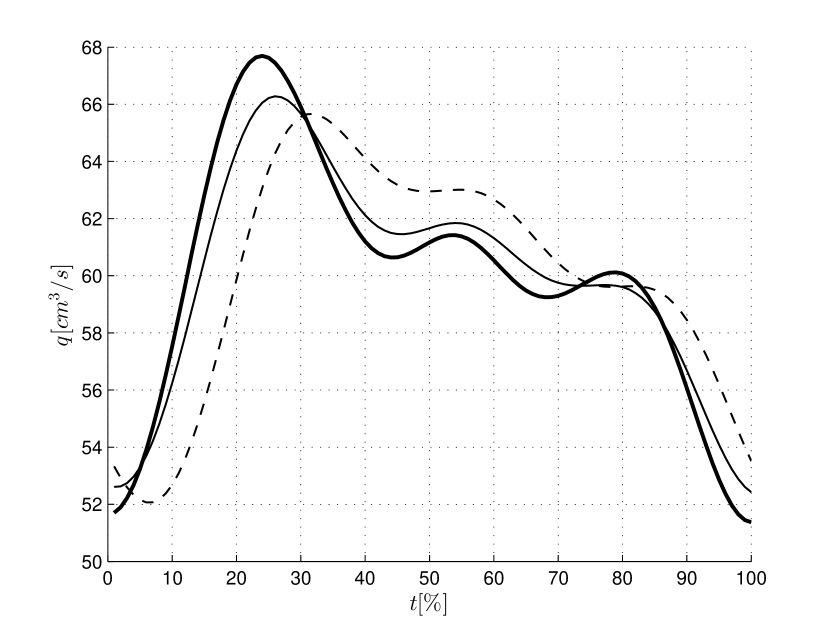
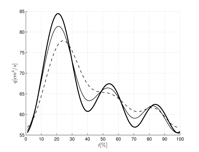
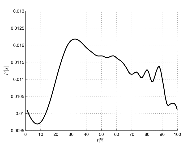
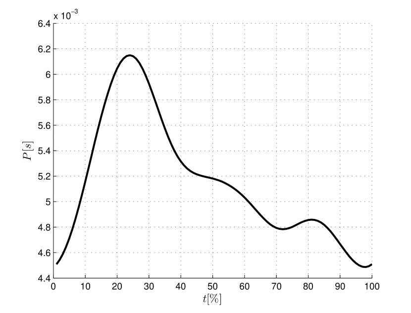
Detailed results are presented for the youngest (patient No. ) and for the oldest patient (patient No. ). Local flow rates were calculated at the , and of the aorta segment. We plot the local flow rates corresponding to the youngest and the oldest patient at different equally distributed times during the cardiac cycle in Fig. 1(a) and Fig. 1(b)).
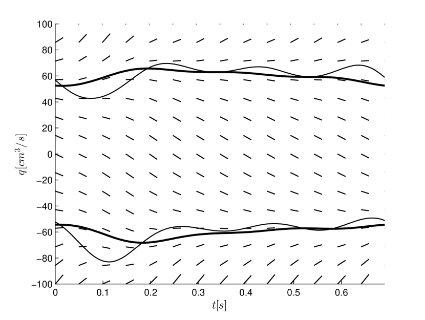
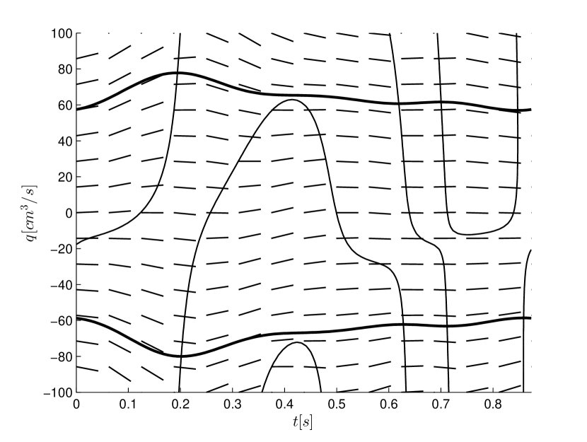
We have seen that conditions of Kotin’s theorem are satisfied in almost all cases and the only exception is just patient No. 5 who was the oldest person. The typical behaviour of the solutions can be seen in Fig. 2(a) and the phase picture corresponding to the only non-typical case is illustrated in Fig. 2(b).
4.2 Reynolds and Womersley numbers
For the sake of completeness, we give the definitions of Reynolds (Re) and Womersley (Wh) numbers. The first is a dimensionless number in fluid mechanics that is defined as the ratio of inertia forces to viscous forces, expressed in tubular flows as
| (20) |
where is the flow velocity, is the vessel’s radius, is the blood density and is the dynamical viscosity of blood. The second is a dimensionless number in biofluid mechanics that relates the transient inertial forces to viscous effects. The Womersley number is defined by
| (21) |
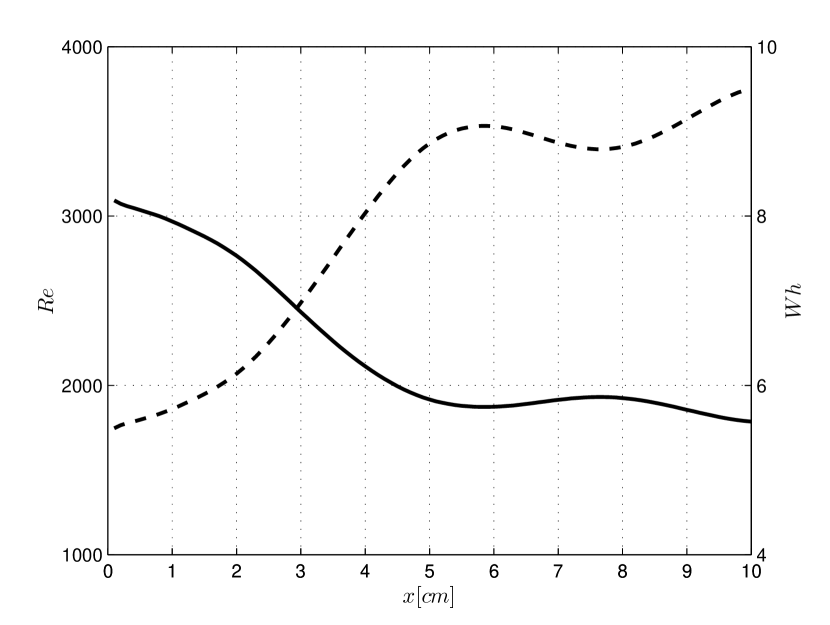
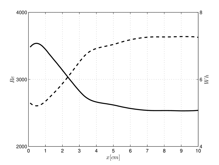
where is the angular frequency of the oscillations. In accordance with the literature [11], [12], in our calculations blood density was set to and the kinematical viscosity of blood to . Estimatons for Reynolds and Womersley numbers along the artery segment are illustrated in common coordinate system in Fig. 4(a) and Fig. 4(b).
The Womersley number is a dynamic similarity measure of oscillatory flows relating inertia and viscous forces. In rigid pipes for laminar incompressible flows small values (approx. Wo1) allow the development of the parabolic velocity profile of the steady state solution and the flow is almost in phase with the pressure gradient, while large values (approx. Wo10) indicate a flat velocity profile with a good approximation and the flow follows the pressure gradient by about 90 degrees in phase. In the presented examples – as seen in Fig. 4(a) and 4(b) – the values lie inbetween, yielding a complex time-dependent velocity profile.
The Reynolds number is another dynamic similarity measure relating inertia and viscous forces. In rigid pipes small values (approx. Re2100) indicate laminar flow, while large values (approx. Re4000) correspond to turbulent flow. In the transition zone, where also our example is situated, the behavior strongly depends on the existing disturbances in the flow.
5 Discussion
Our work present a novel numerical algorithm for the non-invasive blood flow quantification based on ECG-gated CT angiography images.
Quantification of flow in blood vessels provides important information aiding the management of different clinical conditions [13]. Since its introduction in the late 1980s, phase-contrast magnetic resonance (MR) imaging has become the method of choice for flow quantification over ultrasound, as it is able to measure time-resolved 3D flow with high accuracy and reproducibility without the need of a good acoustic window [14]. Our approach enables us to calculate aortic flow on a routine ECG-gated CT angiography dataset. This is of huge clinical potential, as the knowledge of hemodynamic parameters could vastly improve the diagnostic performance of CT imaging in several cardiovascular pathologies, such as aortic coarctation or dissection. Our method can also be beneficial in the management of patients who are not candidates for an MR examination with long acquisition time either because of claustrophobia or due to unstable patient status.
State-of-the-art investigations of the disorders of human arterial sections apply 3D numerical fluid–structure interaction simulations involving the calculation of the blood flow field inside the lumen, the necessary boundary conditions of which are the time-dependent pressure profile at the outlet and volumetric flow rate at the inlet cross-section. The protocol to determine these functions non-invasively is the measurement of both on the arm followed by transforming them to the section under scrutiny by a 1D systemal model of the circulatory system. Our method offers a different and easy to use procedure to formulate the inlet boundary condition without Dopler velocimetry, thus facilitating 3D simulations.
6 Conclusions
We presented a novel numerical algorithm for the non-invasive quantification of blood flow based on ECG-gated CT angiography images. This method can vastly improve the diagnostic performance of CT imaging in several cardiovascular pathologies. Further studies are needed to validate our approach in a clinical setting.
A block-based optimization algorithm was developed to compute local flow rate in time. The wave form of the local flow rate curves seems to be similar to those that can be measured by invasive intraarterial method. The mean squared error (MSE) values, which measures the goodness of the model, are quite small compared to the average flow rate.
According to the analysis of Reynolds and Womersley numbers, the velocity profile has a complex time-dependent behaviour in the detailed examples (Patient No. 3 and No. 5).
We have found that conditions of Kotin’s theorem are satisfied in most of the cases and the physically admissible solution is not assymptotically stable in general. Further mathematical analysis of equation (7) is needed to find weaker sufficient conditions for the physical admissibility.
References
References
- [1] G. S. K. Yunlong Huo, Pulsatile blood flow in the entire coronary arterial tree: theory and experiment, American Journal of Physiology - Heart and Circulatory Physiology 291 (3) (2006) H1074–H1087. doi:10.1152/ajpheart.00200.2006.
- [2] R. G. Moloy Kumar Banerjee, A. Datta, Effect of pulsatile flow waveform and womersley number on the flow in stenosed arterial geometry, ISRN Biomathematics 2012 (11) (2012) 1–17. doi:10.5402/2012/853056.
- [3] S. P. S. Mir Golam Rabby, M. M. Molla, Pulsatile non-newtonian laminar blood flows through arterial double stenoses, Journal of Fluids 2014 (2014) 1–13. doi:10.1155/2014/757902.
- [4] D. T. Michael Kass, Andrew P. Witkin, Snakes: Active contour models, International Journal of Computer Vision 1 (4) (1988) 321–331. doi:10.1007/BF00133570.
- [5] U. J. S. M. F. R. Christoph R. Becker, Bernd M. Ohnesorge, Current development of cardiac imaging with multidetector-row ct, European Journal of Radiology 36 (2) (2000) 97–103. doi:10.1016/S0720-048X(00)00272-2.
- [6] B. A. U. C. A. C. J. L. L. R. S. J. C. C. M. J. H. J. H. L. James P. Earls, Elise L. Berman, Prospectively gated transverse coronary ct angiography versus retrospectively gated helical technique: Improved image quality and reduced radiation dose, Radiology 246 (3) (2008) 742–753. doi:10.1148/radiol.2463070989.
- [7] V. H. Milan Sonka, R. Boyle, Image Processing, Analysis, and Machine Vision, Cengage Learning, 2008, iSBN-10: 1133593607.
- [8] J. K. Tomáš Svoboda, V. Hlaváč, Image Processing, Analysis & and Machine Vision - A MATLAB Companion, Thomson Learning, 2007, iSBN: 0495295957.
- [9] R. Nagy, C. Csobay-Novák, A. Lovas, P. Sótonyi, I. Bojtár, Non-invasive in vivo time-dependent strain measurement method in human abdominal aortic aneurysms: Towards a novel approach to rupture risk estimation, Journal of biomechanics 48 (10) (2015) 1876–1886. doi:doi:10.1016/j.jbiomech.2015.04.030.
- [10] L. Kotin, On positive and periodic solutions of riccati equations, SIAM Journal of Applied Mathematics 16 (6) (1968) 1227–1231. doi:10.1137/0116103.
- [11] K. K. C. M. C. Y. L. H. C. S. L. S. K. D. Jung JM, Lee DH, Reference intervals for whole blood viscosity using the analytical performance-evaluated scanning capillary tube viscometer., Clinical Biochemistry 47 (6) (2014) 489–93. doi:10.1016/j.clinbiochem.2014.01.021.
- [12] G. J. Hinghofer-Szalkay H, Continuous monitoring of blood volume changes in humans., J. Appl. Physiol. (1985) 63 (3) (1987) 1003–7.
- [13] T. C. T. G. A.J. Powell, S.E. Maier, Phase–velocity cine magnetic resonance imaging measurement of pulsatile blood flow in children and young adults: In vitro and in vivo validation, Pediatric Cardiology 21 (2000) 104–110. doi:10.1007/s002469910014.
- [14] J. G. K. B. J. Zoran Stankovic, Bradley D. Allen, M. Marki, 4d flow imaging with mri, Cardiovascular Diagnosis & Therapy 4 (2) (2014) 173–192. doi:10.3978/j.issn.2223-3652.2014.01.02.