Learning with Memory Embeddings

Abstract

Embedding learning, a.k.a. representation learning, has been shown to be able to model large-scale semantic knowledge graphs. A key concept is a mapping of the knowledge graph to a tensor representation whose entries are predicted by models using latent representations of generalized entities. Latent variable models are well suited to deal with the high dimensionality and sparsity of typical knowledge graphs. In recent publications the embedding models were extended to also consider time evolutions, time patterns and subsymbolic representations. In this paper we map embedding models, which were developed purely as solutions to technical problems for modelling temporal knowledge graphs, to various cognitive memory functions, in particular to semantic and concept memory, episodic memory, sensory memory, short-term memory, and working memory. We discuss learning, query answering, the path from sensory input to semantic decoding, and the relationship between episodic memory and semantic memory. We introduce a number of hypotheses on human memory that can be derived from the developed mathematical models. There are four main hypotheses. The first one is that semantic memory is described as triples and that episodic memory is described as triples in time. A second main hypothesis is that generalized entities have unique latent representations which are shared across memory functions and that are the basis for prediction, decision support and other functionalities executed by working memory (tensor memory hypothesis). A third main hypothesis is that the latent representation for a time $t$, which summarizes all sensory information available at time $t$, is the basis for episodic memory. Finally, our proposed model suggests that semantic memory and episodic memory depend on each other: Episodic decoding depends on semantic memory and semantic memory is developed as a long term store of episodic memory. On the other hand there is also a certain independence: the pure storage of episodic memory does not depend on semantic memory and semantic memory can be acquired even without a functioning episodic memory. The same relationships between semantic and episodic memories can be found in the human brain.

1 Introduction

Embedding learning, a.k.a. representation learning, is an essential ingredient of successful natural language models and deep architectures [125, 18, 17, 19, 90, 58] and has been the basis for modelling large-scale semantic knowledge graphs [110, 138, 104, 22, 23, 130, 40, 106, 107]. A key concept is a mapping of the knowledge graph to a tensor representation whose entries are predicted by models using latent representations of generalized entities. Latent variable models are well suited to deal with the high dimensionality and sparsity of typical knowledge graphs. In recent publications the embedding models were extended to also consider temporal evolutions, time patterns and subsymbolic representations [48, 49]. These extended models were used successfully to predict clinical events like procedures, lab measurements, and diagnoses. In this paper, we attempt to map these embedding models, which were developed purely as solutions to technical problems, to various cognitive memory functions. Our approach follows the tradition of latent semantic analysis (LSA), which is a classical representation learning approach that on the one hand has found a number of technical applications and on the other hand could be related to cognitive semantic memories [88, 87, 38].

Cognitive memory functions are typically classified as long-term, short-term, and sensory memory, where long-term memory has the subcategories declarative memory and non-declarative memory [42, 6, 131, 14, 35, 54, 57]. Figure 1 shows these main categories and finer subcategories and shows the role of working memory [9]. There is evidence that these main cognitive categories are partially dissociated from one another in the brain, as expressed in their differential sensitivity to brain damage [54]. However, there is also evidence indicating that the different memory functions are not mutually independent and support each other [76, 61].

The paper is organized as follows. In the next section, we introduce the unique-representation hypothesis as the basis for exchanging information between different memory functions. We present the different tensor representations of the main memory functions and discuss offline learning of the models. In Section 3 we introduce different representations for the indicator mapping function used in the memory models and in Section 4 we show how likely triples can be generated from the model using a simulated-annealing based sampling perspective. In Section 5 we discuss the path from sensory input to a semantic representation of scene information and to long-term semantic and episodic memory. In Section 6 we explain how the different memory representations form the basis of a prediction system and relate this to working memory. Section 7 represents the main results of this paper in form of a discussion of a number of postulated hypotheses for human memory. Section 8 contains our conclusions.

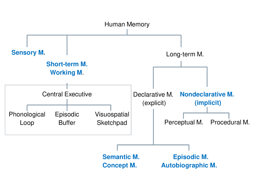
Figure 1: Organization of human memory [54, 57]. In this paper, we discuss the memory functions in blue. Sensory memory, episodic memory and semantic memory will be discussed in most sections. Autobiographic memory is the topic of Subsection 2.4. Working memory and short-term memory are discussed in Sections 6 and Subsection 7.11. Compare Figures 2 and 10.

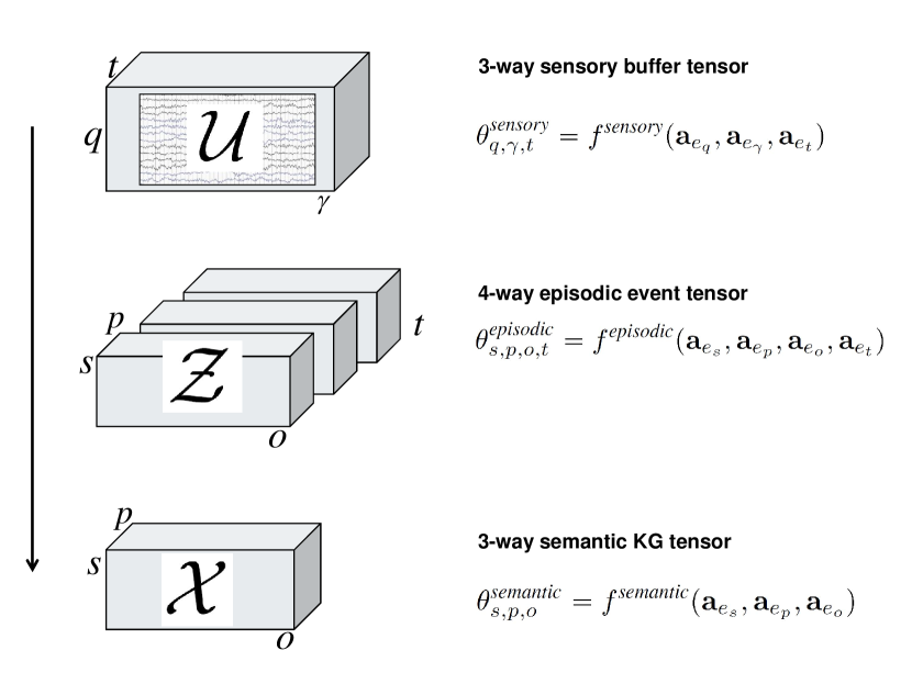
Figure 2: The figure shows the different tensor memories and their models. On the top we see the sensory memory tensor $\mathcal{U}$ with dimensions sensory channel $q$, within buffer position $\gamma$, and time $t$. The time dimension is shared with the episodic event tensor tensor $\mathcal{Z}$ with additional dimensions subject $s$, predicate $p$, and object $o$. The latter three are shared with the semantic KG tensor $\mathcal{X}$. On the right side we show the indicator mapping functions, which are functions of latent representations of the involved generalized entities.

2 Memories and Their Tensor Embeddings

2.1 Unique-Representation Hypothesis

In this section we discuss how the different memory functions can be coded as tensors and how inference and generalization can be achieved by coupled tensor decompositions.

We begin by considering declarative memories. The prime example of a declarative memory is the semantic memory which stores general world knowledge about entities. Second, there is concept memory which stores information about the concepts in the world and their hierarchical organization. In contrast to the general setting in machine learning, in this paper entities are the prime focus and concepts are of secondary interest. Finally, episodic memory stores information of general and personal events [139, 140, 141, 54]. Whereas semantic memory concerns information we “know”, episodic memory concerns information we “remember” [57]. The portion of episodic memory that concerns an individual’s life involving personal experiences is called autobiographic memory.

Semantic memories and episodic memories are long-term memories. In contrast, we also consider sensory memory, which is the shortest-time element of memory. It is the ability to retain impressions of sensory information after the original stimuli have ended [54].

Finally, working memory is the topic of Section 6. Working memory uses the other memories for tasks like prediction, decision support and other high-level functions.

The unique-representation hypothesis assumed in this paper is that each entity or concept $e_{i}$, each predicate $e_{p}$ and each time step $e_{t}$ has a unique latent representation —$\mathbf{a}_{i}$, $\mathbf{a}_{p}$, respectively, $\mathbf{a}_{t}$— in form of a vector of real numbers. The assumption is that the representations are shared between all memory functions, and this permits information exchange and inference between the different memories. For simplicity we assume that the dimensionalities of these latent representations are all identical $\tilde{r}$ such that $\mathbf{a}_{i}\in\mathbb{R}^{\tilde{r}}$, $\mathbf{a}_{p}\in\mathbb{R}^{\tilde{r}}$, and $\mathbf{a}_{t}\in\mathbb{R}^{\tilde{r}}$. Figure 3 shows a simple network realization.

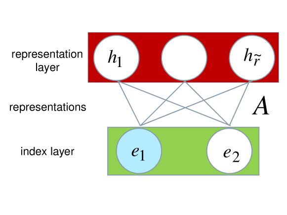
Figure 3: A graphical view of the unique-representation hypothesis. The model can operate bottom up and top down. In the first case, index neurons $e_{i}$ activate the representation layer via their latent representations, implemented as weight vectors. In the figure $e_{1}$ is active, all other neurons are inactive and the representation layer is activated with the pattern $\mathbf{h}=\mathbf{a}_{e_{1}}$. In top-down operation, a representation layer can also activate index neurons. The activation of neuron $e_{i}$ is then the inner product $\mathbf{a}_{e_{i}}^{\top}\mathbf{h}$. We consider here formalized neurons which might actually be implemented as ensembles of neurons or in other form. Here and in the following we assume that the matrix $A$ stores the latent representations of all generalized entities. The context makes it clear if we refer to the latent representations of entities, predicates, or time.

2.2 A Semantic Knowledge Graph Model

A technical realization of a semantic memory is a knowledge graph (KG) which is a triple-oriented knowledge representation. Popular large-scale KGs are DBpedia [7], YAGO [134], Freebase [21], NELL [27], and the Google Knowledge Graph [126].

Here we consider a slight extension to the subject-predicate-object triple form by adding the value in the form ($e_{s},e_{p},e_{o}$; Value) where Value is a function of $s,p,o$ and, e.g., can be a Boolean variable (True or 1, False or 0) or a real number. Thus (Jack, likes, Mary; True) states that Jack (the subject or head entity) likes Mary (the object or tail entity). Note that $e_{s}$ and $e_{o}$ represent the entities for subject index $s$ and object index $o$. To simplify notation we also consider $e_{p}$ to be a generalized entity associated with predicate type with index $p$. We encode attributes also as triples, mostly to simplify the discussion.

We now consider an efficient representation of a KG. With this representation, it is also possible to generalize from known facts to new facts (inductive inference). First, we introduce the three-way semantic adjacency tensor $\mathcal{X}$ where the tensor element $x_{s,p,o}$ is the associated Value of the triple ($e_{s},e_{p},e_{o}$). Here $s=1,\ldots,S$, $p=1,\ldots,P$, and $o=1,\ldots,O$. One can also define a companion tensor $\underline{\Theta}$ with with the same dimensions as $\mathcal{X}$ and with entries $\theta_{s,p,o}$. It contains the natural parameters of the model and the connection to $\mathcal{X}$ for Boolean variables is

$$P(x_{s,p,o}|\theta_{s,p,o})=\textrm{sig}(\theta_{s,p,o})$$ (1)

where $\textrm{sig}(arg)=1/(1+\exp(-arg))$ is the logistic function (Bernoulli likelihood) . If $x_{s,p,o}$ is a real number then we can use a Gaussian distribution with $P(x_{s,p,o}|\theta_{s,p,o})\sim{\mathcal{N}}(\theta_{s,p,o},\sigma^{2})$. Unless specified otherwise, we will assume a Bernoulli distribution for the rest of the paper.

As mentioned, the key concept in embedding learning is that each entity $e$ has an $\tilde{r}$-dimensional latent vector representation $\mathbf{a}\in\mathbb{R}^{\tilde{r}}$. In particular, the embedding approaches used for modeling KGs assume that

$$\theta^{\textit{semantic}}_{s,p,o}=f^{\textit{semantic}}(\mathbf{a}_{e_{s}},\mathbf{a}_{e_{p}},\mathbf{a}_{e_{o}}).$$ (2)

Here, the function $f^{\textit{semantic}}(\cdot)$ predicts the value of the natural parameter. In the case of a KG with a Bernoulli likelihood, $\textrm{sig}(\theta^{\textit{semantic}}_{s,p,o})$ represents the confidence that the Value of the triple ($e_{s},e_{p},e_{o}$) is true and we call the function an indicator mapping function and we discuss examples in the next section.

Latent representation approaches have been used very successfully to model large KGs, such as the YAGO KG, the DBpedia KG and parts of the Google KG. It has been shown experimentally that models using latent factors perform well in these high-dimensional and highly sparse domains. Since an entity has a unique representation, independent of its role as a subject or an object, the model permits the propagation of information across the KG. For example if a writer was born in Munich, the model can infer that the writer is also born in Germany and probably writes in the German language [104, 105]. Stochastic gradient descent (SGD) is typically being used as an iterative approach for finding both optimal latent representations and optimal parameters in $f^{\textit{semantic}}(\cdot)$ [106, 85]. For a recent review, please consult [106].

Due to the approximation, $\textrm{sig}(\theta^{\textit{semantic}}_{\textit{Jack},\textit{marriedTo},e})$ might be smaller than one for the true spouse. The approximation also permits inductive inference: We might get a large $\textrm{sig}(\theta^{\textit{semantic}}_{\textit{Jack},\textit{marriedTo},e})$ also for persons $e$ that are likely to be married to Jack and $\textrm{sig}(\theta^{\textit{semantic}}_{s,p,o})$ can, in general, be interpreted as a confidence value for the triple $(e_{s},e_{p},e_{o})$. More complex queries on semantic models involving existential quantifier are discussed in [84].

A concept memory would technically correspond to classes with a hierarchical subclass structure. In [103, 102] such a structure was learned from the latent representations by hierarchical clustering. In KGs, a hierarchical structure is described by type and subclass relations.

Latent representations for modeling semantic memory functions have a long history in cognitive modeling, e.g., in latent semantic analysis [87] which is restricted to attribute-based representations. Generalizations towards probabilistic models are probabilistic latent semantic indexing [72] and latent Dirichlet allocation [20]. Latent clustering and topic models [78, 146, 2] are extensions toward multi-relational domains and use discrete latent representations. See also [93, 62, 63]. Spreading activation is the basis of the teachable language comprehender (TLC), which is a network model of semantic memory [30]. Associate models are the symbolic ACT-R [4, 5] and SAM [114]. [107] explores holographic embeddings with representation learning to model associative memories. An attractive feature here is that the compositional representation has the same dimensionality as the representation of its constituents. Connectionists memory models are described in [73, 96, 28, 82, 67, 68].

2.3 An Event Model for Episodic Memory

Whereas a semantic KG model reflects the state of the world, e.g, of a clinic and its patients, observations and actions describe factual knowledge about discrete events, which, in our approach, are represented by an episodic event tensor. In a clinical setting, events might be a prescription of a medication to lower the cholesterol level, the decision to measure the cholesterol level and the measurement result of the cholesterol level; thus events can be, e.g., actions, decisions and measurements.

The episodic event tensor is a four-way tensor $\mathcal{Z}$ where the tensor element $z_{s,p,o,t}$ is the associated Value of the quadruple ($e_{s},e_{p},e_{o},e_{t}$). The indicator mapping function then is

$$\theta^{\textit{episodic}}_{s,p,o,t}=f^{\textit{episodic}}(\mathbf{a}_{e_{s}},\mathbf{a}_{e_{p}},\mathbf{a}_{e_{o}},\mathbf{a}_{e_{t}})$$

where we have added a representation for the time of an event by introducing the generalized entity $e_{t}$ with latent representation $\mathbf{a}_{e_{t}}$. This latent representation compresses all events that happen at time $t$.

As examples, the individual can recall “Who did I meet last week?” by $e_{o}=\operatorname*{arg\,max}_{e}\theta^{\textit{episodic}}_{\textit{Myself},\textit{meet},e,\textit{LastWeek}}$ and “When did I meet Jack?” by $e_{t}=\operatorname*{arg\,max}_{e}\theta^{\textit{episodic}}_{\textit{Myself},\textit{meet},\textit{Jack},e}$.

Examples from our clinical setting would be: (Jack, orderBloodTest, Cholesterol, Week34; True) for the fact that a cholesterol blood test was ordered in week 34 and (Jack, hasBloodTest, Cholesterol, Week34; 160) for the result of the blood test. Note that we consider an episodic event memory over different subjects, predicates and objects; thus episodic event memory can represent an extensive event context!

An event model can be related to the cognitive concept of an episodic memory (Figure 1). Episodic memory represents our memory of experiences and specific events in time in a serial form (a “mental time travel”), from which we can reconstruct the actual events that took place at any given point in our lives [127]. In contrast to semantic memory, it requires recollection of a prior experience [140].

For a particular instance in time $t$, the “slice” of the event tensor $\mathcal{Z}_{t}$ describes events as a, typically very sparse, triple graph. Some of the elements of this triple graph will affect changes in the KG [48, 49] (see also the discussion in Section 7). For example the event model might record a diagnosis which then becomes a fact in the KG. Also the common representations for subject, predicate, and object lead to a transfer from the event model to the semantic KG model (see also the discussion in Section 7).

2.4 Autobiographical Event Tensor

In some applications we want to consider the episodic information specific to an individual. For example, in a patient model, one is interested in what happened to the individual at time $t$ and not what happened to all patients at time $t$. The autobiographical event tensor is simply the sub-tensor $\mathcal{Z}_{s}$ concerning the events of the individual only. We then obtain a personal time $e_{s=i,t}$ with latent representation $\mathbf{a}_{e_{s=i,t}}$. Whereas $\mathbf{a}_{e_{t}}$ is a latent representation for all events for all patients at time $t$, $\mathbf{a}_{e_{s=i,t}}$ is a latent representation for all events for patients $i$ at time $t$ [48, 49].

The autobiographical event tensor would correspond to the autobiographical memory, which stores autobiographical events of an individual on a semantic abstraction level [33, 54]. The autobiographical event tensor can be related to Baddeley’s episodic buffer and, in contrast to Tulving’s concept of episodic memory, is a temporary store and is considered to be a part of working memory [10, 76, 11].

2.5 A Sensory Buffer

We assume that the sensor input consists of $Q$-channels and that at each time step $t$ a buffer is constructed of $N$ samples of the $Q$ channels. $\gamma=0,\ldots,N$ specifies the time location within the buffer (see also Figure 2). In contrast to the event buffer, the sensory buffer operates at a subsymbolic level. Technically it might represent measurements like temperature and pressure, and in a cognitive model, it might represent input channels from the senses. The sensory buffer might be related to the mini-batches in Spark Streaming where data is captured in buffers that hold seconds to minutes of the input streams [149].

The sensory buffer is described by a three-way tensor $\mathcal{U}$ where the tensor element $u_{q,\gamma,t}$ is the associated Value of the triple ($e_{q},e_{\gamma},e_{t}$). $e_{q}$ is a generalized entity for the $q$-th sensory channel, $e_{\gamma}$ specifies the time location in the buffer and $e_{t}$ is a generalized entity representing the complete buffer at time $t$.

We model

$$\theta^{\textit{sensory}}_{q,\gamma,t}=f^{\textit{sensory}}(\mathbf{a}_{e_{q}},\mathbf{a}_{e_{\gamma}},\mathbf{a}_{e_{t}})$$

where $\mathbf{a}_{e_{q}}$ is the latent representations for the sensor channel $e_{q}$ and $\mathbf{a}_{e_{\gamma}}$ is the latent representations for $e_{\gamma}$. Latent components corresponds to complex time patterns (chunks) whose amplitudes are determined by the components of $\mathbf{a}_{e_{t}}$; thus complex sensory events and sensory patterns can be modelled.

In a technical application [49], the sensors measure, e.g., wind speed, temperature, and humidity at the location of wind turbines and the sensory memory retains the measurements from $t-1$ to $t$.

In human cognition, sensory memory (milliseconds to a second) represents the ability to retain impressions of sensory information after the original stimuli have ended [139, 31, 54]. The transfer of sensory memory to short-term memory (e.g., the autobiographical episodic buffer) is the first step in some memory models, in particular in the modal theory of Atkinson and Shiffrin [6]. New evidence suggests that short-term memory is not the sole gateway to long-term memory [54]. Sensory memory is thought to be located in the brain regions responsible for the corresponding sensory processing. Sensory memory can be the basis for sequence learning and the detection of complex time patterns.

2.6 Comment

The different memories and their tensor representations and models are summarized in Figure 2. Under the unique-representation hypothesis assumed in this paper, the latent representations of generalized entities are central for retrieval and prediction: the memory does not need to store all the facts and relationships about an entity. Also, there is no need to explicitly store the semantic graph explicitly. At any time, an approximation to the graph can be reconstructed from the latent representations. See also the discussion in Section 7.

2.7 Cost Functions

Each memory function generates a term in the cost function (see Appendix) and all terms can be considered in training to adapt all latent representations and all parameters in the various functional mappings. Note that this is a global optimization step involving all available data. In general, we assumed a unique-representation for an entity, for example we assume that ${\mathbf{a}}_{e_{s}}$ is the same in the prediction model and in the semantic model. Sometimes it makes sense to relax that assumption and only assume some form of a coupling. Technically there are a number of possibilities: For example, the prediction model might be trained on its own cost function, using the latent representations from the knowledge graph as an initialization; alternatively, one can use different weights for the different cost function terms. Some investigators propose that only some dimensions of the latent representations should be shared [3, 1]. [89, 19, 17] contain extensive discussions on the transfer of latent representations. It is important to note that by considering only conditional probability models (e.g., Value, conditioned on subject, predicate and object), no global normalization needs to be considered in training.

3 Modelling the Indicator Mapping Function

3.1 Using General Function Approximators

Consider the semantic KG. Here, the indicator mapping function $f^{\textit{semantic}}(\cdot)$ can be modelled as a general function approximator, such as a feedforward “multiway” neural network (NN), where the index neurons representing $e_{s}$, $e_{p}$, and $e_{o}$ are activated at the input and the response is generated at the output, as shown in the top of Figure 4. With this model it would be easy to query for the plausibility of a triple $(e_{s},e_{p},e_{o};\textit{Value})$, but other queries would be more difficult to handle.

An alternative model is shown at the bottom of Figure 4 with inputs $e_{s}$ and $e_{p}$ and where a function approximator predicts a latent representation vector $\mathbf{h}^{\textit{object}}$ with components

$$h^{\textit{object}}_{r}={f}_{r}^{\textit{semantic, object}}(\mathbf{a}_{e_{s}},\mathbf{a}_{e_{p}})\;\;\;\;\;\;r=1,\ldots,\tilde{r}.$$

The function $f^{\textit{semantic}}(\cdot)$ is now calculated as an inner product between the predicted latent representation and the latent representation of the objects as

$$f^{\textit{semantic}}(\mathbf{a}_{e_{s}},\mathbf{a}_{e_{p}},\mathbf{a}_{e_{o}})=\mathbf{a}_{e_{o}}^{\top}\mathbf{f}^{\textit{semantic, object}}(\mathbf{a}_{e_{s}},\mathbf{a}_{e_{p}})=\mathbf{a}_{e_{o}}^{\top}\mathbf{h}^{\textit{object}}.$$ (3)

Here, $\mathbf{f}^{\textit{semantic, object}}=({f}_{1}^{\textit{semantic, object}},\ldots,{f}_{\tilde{r}}^{\textit{semantic, object}})^{\top}$.

Thus the response to the query $(\textit{Jack},\textit{likes},?)$ can be obtained by activating the index neurons for Jack and likes at the input and by considering index neurons at the outputs with large values. Note that with $\mathbf{f}=\mathbf{{f}}^{\textit{semantic, object}}(\cdot)$, a function approximator produces a latent representation vector $\mathbf{h}$ and the activation of the output index neurons corresponds to the likelihood that $e_{o}$ is the right answer. We call this modelling approach indicator mapping by representation prediction.

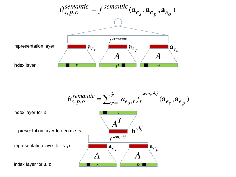
Figure 4: Indicator mapping function (top): The index neurons representing $e_{s}$, $e_{p}$, and $e_{o}$ are activated at the input and the indicator mapping function is generated at the output. Indicator mapping prediction using representation prediction (bottom): With inputs $e_{s}$ and $e_{p}$, a latent representation vector $\mathbf{h}^{\textit{object}}$ is calculated which activates the output index neurons encoding the objects.

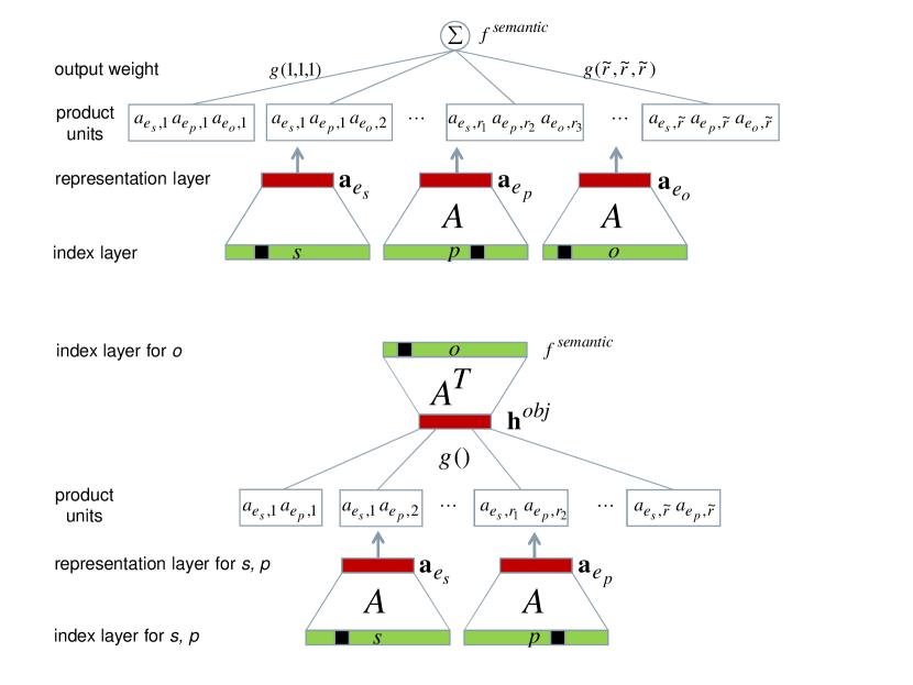
Figure 5: As in Figure 4 but with a Tucker model. Top: An architecture with two hidden layers, Interaction between latent representations are implemented by the product nodes. Bottom: Same but drawn as a model with three hidden layers. The $g(\cdot)$-layer fully connects the outputs of the product layer with the object representation layer. Since the Tucker model is symmetrical with respect to the generalized entities, in the following we draw all representations below the $g(\cdot)$-layer.

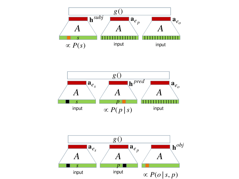
Figure 6: For nonnegative tensor models, marginals and conditionals can easily be calculated and independent samples from the model can be calculated. The figure shows the situation for a Tucker model. In the top model, we apply vectors of ones to the predicate and object representation, which leads to a marginalization of those variables. The subject representation acts as output and we can sample a subject. In the center, we only integrate out the object and use the subject index as input. At the predicate output we can sample a predicate. Finally, in the bottom, we use subject and predicate samples as inputs and produce a sample for an object. Naturally, when subject and predicate are given, we only need to use the model at the bottom.

3.2 Tensor Decompositions

Tensor decompositions have also shown excellent performance in modelling KGs [106]. In tensor decompositions, the indicator mapping function $f^{\textit{semantic}}(\cdot)$ is implemented as a multilinear model.

Of particular interest are the PARAFAC model (canonical decomposition) with

$$f^{\textit{semantic}}(\mathbf{a}_{e_{s}},\mathbf{a}_{e_{p}},\mathbf{a}_{e_{o}})=\sum_{r=1}^{\tilde{r}}{a}_{e_{s},r}\;{a}_{e_{p},r}\;{a}_{e_{o},r}$$

and the Tucker model with

$$f^{\textit{semantic}}(\mathbf{a}_{e_{s}},\mathbf{a}_{e_{p}},\mathbf{a}_{e_{o}})=\sum_{r_{1}=1}^{\tilde{r}}\sum_{r_{2}=1}^{\tilde{r}}\sum_{r_{3}=1}^{\tilde{r}}{a}_{e_{s},r_{1}}\;{a}_{e_{p},r_{2}}\;{a}_{e_{o},r_{3}}\;g(r_{1},r_{2},r_{3}).$$

Here, $g(r_{1},r_{2},r_{3})\in\mathbb{R}$ are elements of the core tensor $\mathcal{G}\in R^{\tilde{r}\times\tilde{r}\times\tilde{r}}$. Finally, the RESCAL model [104] is a Tucker2 model with

$$f^{\textit{semantic}}(\mathbf{a}_{e_{s}},\mathbf{a}_{e_{p}},\mathbf{a}_{e_{o}})=\sum_{r_{1}=1}^{\tilde{r}}\sum_{r_{2}=1}^{\tilde{r}}{a}_{e_{s},r_{1}}\;{a}_{e_{o},r_{2}}\;g(r_{1},r_{2},e_{p})$$

with core tensor $\mathcal{G}\in R^{\tilde{r}\times\tilde{r}\times{P}}$. In all these models, we use the constraint that a generalized entity has a unique latent representation.

An attractive feature of tensor decompositions is that, due to their multilinearity, representation prediction models can easily be constructed: For the PARAFAC model, $h^{\textrm{object}}_{r}={a}_{e_{s},r}\;{a}_{e_{p},r}$, for Tucker, $h^{\textrm{object}}_{r}=\sum_{r_{1}=1}^{\tilde{r}}\sum_{r_{2}=1}^{\tilde{r}}{a}_{e_{s},r_{1}}{a}_{e_{p},r_{2}}\;g(r_{1},r_{2},r)$ and for RESCAL $h^{\textrm{object}}_{r}=\sum_{r_{1}=1}^{\tilde{r}}{a}_{e_{s},r_{1}}\;\;g(r_{1},r,e_{p})$. The architectures for the Tucker model are drawn in Figure 5.

4 Querying Memories

4.1 Function Approximator Models

In many application one is interested in retrieving triples with a high likelihood, conditioned on some information, thus we are essentially faced with an optimization problem. To answer a query of the form $(\textit{Jack},\textit{likes},?)$ we need to solve

$$\arg\max_{\mathbf{a}_{e_{o}}}f^{\textit{semantic}}(\textit{Jack},\textit{likes},\mathbf{a}_{e_{o}}).$$

Of course one is often interested in a set of likely answers.

We suggest to address querying via a simulated annealing approach. We define an energy function $E(s,p,o)=-f^{\textit{semantic}}(\mathbf{a}_{e_{s}},\mathbf{a}_{e_{p}},\mathbf{a}_{e_{o}})$ and define a Boltzmann distribution as

$$P(s,p,o)=\frac{1}{Z(\beta)}\exp\beta f^{\textit{semantic}}(\mathbf{a}_{e_{s}},\mathbf{a}_{e_{p}},\mathbf{a}_{e_{o}}).$$

Here $Z(\beta)$ is the partition function that normalizes the distribution and $\beta\geq 0$ is an inverse temperature. Note that we now have generated a probability distribution where subject, predicate, and object are the random variables!

Now to answer the query, $(\textit{Jack},\textit{likes},?)$, we sample from

$$P(o|s,p)=\frac{1}{Z(s,p,\beta)}\exp\beta f^{\textit{semantic}}(\mathbf{a}_{e_{s}},\mathbf{a}_{e_{p}},\mathbf{a}_{e_{o}})$$

with $s=\textit{Jack}$ and $p=\textit{likes}$. The artificial inverse temperature $\beta\geq 0$ can determine if we are interested in just sampling the most likely response (large $\beta$) or are also interested in responses with a smaller probability (small $\beta$). Similarly, we can derive models for $P(s|p,o)$ and $P(p|s,o)$.

4.2 Tensor Models

By enforcing nonnegativity of the factors and the core tensor entries, we can define a probabilistic model for a Tucker model with $E(s,p,o)=-\log f^{\textit{semantic}}(\mathbf{a}_{e_{s}},\mathbf{a}_{e_{p}},\mathbf{a}_{e_{o}})$ as

$$P(s,p,o)\propto\left(\sum_{r_{1}=1}^{\tilde{r}}\sum_{r_{2}=1}^{\tilde{r}}\sum_{r_{3}=1}^{\tilde{r}}{a}_{e_{s},r_{1}}\;{a}_{e_{p},r_{2}}\;{a}_{e_{o},r_{3}}\;g(r_{1},r_{2},r_{3})\right)^{\beta}.$$ (4)

An attractive feature of tensor models is that marginals and conditionals can easily be obtained. Here, we look at the Tucker model. For $P(o|s,p)$ we we can use the Equation 4 with appropriate normalization. For $P(p|s)$ we use the same equation where we replace ${\mathbf{a}}_{e_{o}}$ with $\mathbf{\bar{{a}}}^{\textit{object}}=\sum_{o}{\mathbf{a}}_{e_{o}}$. For $P(s)$ we use the same equation again where we replace in addition ${\mathbf{a}}_{e_{p}}$ with $\mathbf{\bar{{a}}}^{\textit{predicate}}=\sum_{p}{\mathbf{a}}_{e_{p}}$. As shown in the architecture in Figure 6, these operations can easily be implemented. Marginalization means that the index neurons are all active, indicated by the vector of ones in the figure.

We can use these models to generate samples from the distribution by first generating a sample for $s$ from $P(s)$, then a sample from $p$ from $P(p|s)$, and finally a sample from $o$ using $P(o|s,p)$. By repeating this process we can obtain independent samples from $P(s,p,o)$!

Note that there is a certain equivalence between tensor models and sum-product networks, where similar operations for marginals and conditionals can be defined [111].

We can generalize the approach to all memory functions by defining suitable energy functions. We want to emphasize that we use the probability distributions only for query-answering and not for learning!

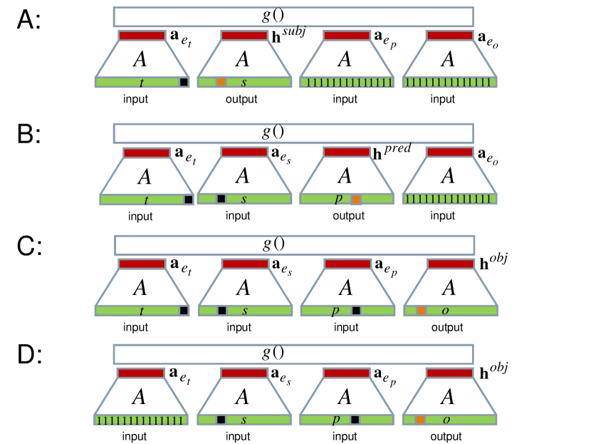
Figure 7: The semantic decoding using a 4-dimensional Tucker tensor model. A: $\mathbf{a}_{e_{t}}$ is generated by the mapping of the sensory buffer by $\mathbf{f}^{M}(\cdot)$. To sample a subject $s$ given time $t$, predicate $p$ and object $o$ are marginalized. B: Here, $o$ is marginalized and one samples a predicate $p$, given $t,s$. C: Sampling of an object $o$, given $t,s,p$. D: By integrating out the time dimension, we obtain a memory, which is a particular semantic memory. For marginalization, one can either input a vector of ones (as shown) or one learns a mean representation vector $\mathbf{\bar{a}}$.

5 From Sensory Memory to Semantic Decoding

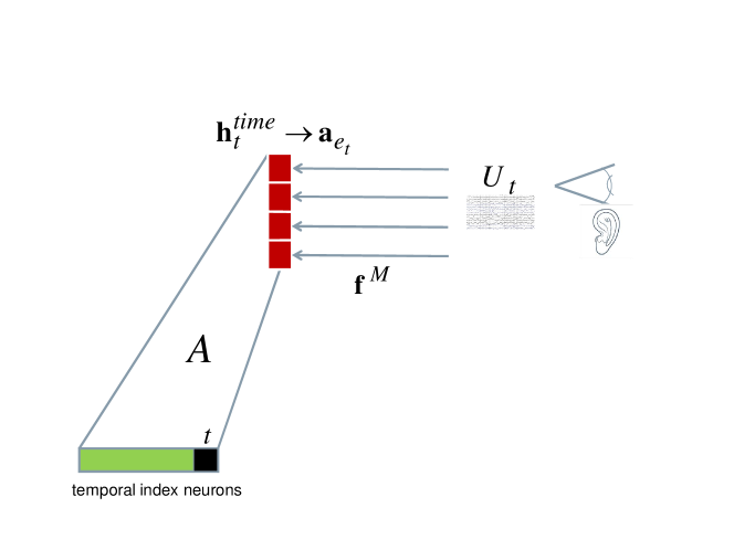
Figure 8: Mapping of $U_{t}=u_{:,:,t}$, i.e., the sensory input at time $t$, to the latent representation for time $\mathbf{h}_{t}^{\textit{time}}$ by the function $\mathbf{f}^{M}(\textrm{vec}(u_{:,:,t}))$. If the sensory input is significant, e.g. novel, unexpected or attached with emotions, then the time index neuron $e_{t}$ is generated which stores $\mathbf{h}_{t}^{\textit{time}}$ as the latent representation $\mathbf{a}_{e_{t}}$. These then eventually become part of the long-term episodic memory. As indicated, $\mathbf{f}^{M}(\cdot)$ might consist of several sub-functions which extract different latent features.

We now consider the situation that a new sensor input becomes available for time $t$. With all other latent representations and functional mappings fixed, the challenge is to calculate a new latent representation $\mathbf{h}_{t}^{\textit{time}}$. Since for a new sensory input at time $t$, the only available information is the sensory buffer $u_{:,:,t}$ there is a clear information propagation from sensory input to the episodic memory. We assume a nonlinear map of the form

$$\mathbf{h}_{t}^{\textit{time}}=\mathbf{f}^{M}(\textrm{vec}(u_{:,:,t}))$$ (5)

where $\mathbf{f}^{M}(\cdot)$ is a function to be learned [147] (see Figure 8) and where $\textrm{vec}(u_{:,:,t})$ are vectorized representations from the portion of the sensory tensor associated with the individual at time $t$. Depending on the application, $\mathbf{f}^{M}(\cdot)$ can be a simple linear map, or it can be a second to last layer in a deep neural network as in the face recognition application DeepFace [136, 101]. In general, we assume that $\mathbf{f}^{M}(\cdot)$ is realized by a set of functions, where each function focusses on different aspects of the sensory inputs (Figure 8). For example, if the sensory input is an image, one function might analyse color, another ones shape and a third one texture.

One can think of $\mathbf{h}_{t}^{\textit{time}}$ as the latent representation of a query; the decoding in the semantic decoder then corresponds to the answer to the query.

Assuming that a Tucker model is used for decoding, the conditional probability becomes

$$P(s,p,o|\textrm{vec}(u_{:,:,t}))\propto\left(\sum_{r_{1}=1}^{\tilde{r}}\sum_{r_{2}=1}^{\tilde{r}}\sum_{r_{3}=1}^{\tilde{r}}\sum_{r_{4}=1}^{\tilde{r}}{a}_{e_{s},r_{1}}\;{a}_{e_{p},r_{2}}\;{a}_{e_{o},r_{3}}\;{h}_{t,r_{4}}\;g(r_{1},r_{2},r_{3},r_{4})\right)^{\beta}.$$ (6)

A sampling approach for decoding with a Tucker model is shown in Figure 7.

For general function approximators one needs to train separate models for the different conditional and marginal probabilities, as discussed in Subsection 9.2 (Figure 12).

Note that in the decoding step we transfer information from a subsymbolic sensory representation to a symbolic semantic representation.

Also note that, in pure perception, no learning of any kind needs to be involved. Only when the sensory input is significant, e.g. novel, unexpected or attached with emotions, then the time index neuron $e_{t}$ is generated which stores $\mathbf{h}_{t}^{\textit{time}}$ as its latent representation $\mathbf{a}_{e_{t}}$. By this operation an episode or event is generated. The time index neuron and its latent representation are eventually transferred to long-term episodic memory (Figure 8).

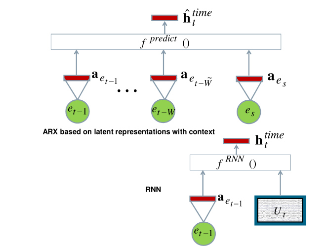
Figure 9: Two different prediction models. In the ARX model on top, we assume that $\mathbf{\hat{h}}$ is a deterministic function of the sensory input $u_{:,:,t}$ and not of past latent states. Time dependencies on $u_{:,:,t}$ are reflected in time dependencies on the latent states $\mathbf{\hat{h}}$ and thus future values of the latent states can be predicted using past latent states. The RNN on the bottom corresponds to the dependencies typically used in recurrent neural networks and state space models. Here past latent states causally influence future latent states.

6 Predictions with Memory Embeddings and Working Memory

In this section we focus on working memory, which orchestrates the different memory functions, e.g. for prediction and decision making. In a way working memory represents the intelligence on top of the memory functions and links to complex decision making and consciousness have been made. Here we will focus on the restricted but important task of prediction. For example, in a clinical setting, it is important to know what should be done next (e.g., prediction of a medical procedure) or what event will happen next (e.g., prediction of a medical diagnosis).

We propose that prediction should be happen at the level of the latent representation for time, i.e., $\mathbf{\hat{h}}$, which is the output of the sensory map, and we consider two cases.

6.1 ARX Model for Predicting Latent Representations of Time

Here we assume that $\mathbf{\hat{h}}$ is a deterministic function of the sensory input via Equation 5 but not of past time latent representations. There might be time dependencies in the sensory input; due to high dimensionality of the input, it is easier to model the dependencies between the latent representations instead, as

$$\mathbf{\hat{h}}_{t}^{\textit{time}}=\mathbf{f}^{\textit{predict}}(\mathbf{a}_{e_{t-1}},\mathbf{a}_{e_{t-2}},\ldots,\mathbf{a}_{e_{t-W}},\mathbf{a}_{e_{\textit{indiviual}}}).$$

But note that this model is only used for prediction $\mathbf{h}_{t}^{\textit{time}}$ and as soon as the sensory input is available, it overrides the prediction with Equation 5! The model is also suitable for novelty detection: if $\mathbf{\hat{h}}$ is different from $\mathbf{h}_{t}^{\textit{time}}$, then the sensory scene might be novel.

Note that we also include the latent representation of the individual $\mathbf{a}_{e_{\textit{indiviual}}}$ which can be interpreted as a representation of the state of the individual.

The model can be interpreted as an autoregressive model on the latent representations with external inputs, ARX (Figure 9, top). The parameter $\tilde{W}$ is the size of the time window and might be related to the capacity of short-term memory, i.e., the number of items the working memory can consider in decision making.

6.2 Recurrent Model

Here we extend the model is Equation 7 to include past information of the latent representation as

$$\mathbf{h}_{t}^{\textit{time}}=\mathbf{f}^{RNN}(\textrm{vec}(u_{:,:,t}),\mathbf{a}_{e_{t-1}},\mathbf{a}_{e_{\textit{indiviual}}}).$$ (7)

Note that this is the structure of a recurrent neural network and the assumption is that the latent state depends on both sensory input and the previous latent state. The architecture is shown in Figure 9, bottom.

Both models are reasonable for different purposes and make different assumptions. In fact, both models might play a role in human cognition.

Alternatively one might use networks with additional memory buffers and attention mechanisms [71, 143, 60, 86, 58].

7 Hypotheses on Human Memory

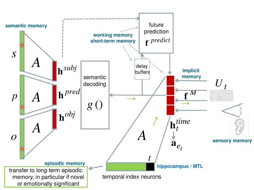
Figure 10: A model for human memory. First consider the semantic decoding step. $U_{t}=u_{:,:,t}$ is the sensory buffer at time $t$. $\mathbf{f}^{M}(\cdot)$ maps the sensory buffer to $\mathbf{h}_{t}^{\textit{time}}$. As discussed before, this function might be realized by a set of modules where each module focusses on certain aspects of the sensory input. If the memory is novel or emotionally significant, a new episodic memory is formed by the generation of time index neuron $e_{t}$; its latent representation is then stored as weight pattern $\mathbf{a}_{e_{t}}=\mathbf{h}_{t}^{\textit{time}}$. The index neuron and the representations can eventually become part of long-term episodic memory. The semantic decoding module (here: Tucker tensor model) then produces highly probable $(s,p,o)$-triples, given $\mathbf{h}_{t}^{\textit{time}}$ and as described in Figure 7. Semantic decoding also also performed when no episodic memory is formed. A form of a semantic memory can be achieved by marginalizing time. It is even possible to operate the model in reverse: If we consider $s$ to be the input, let’s say Mary, marginalize out $p$ and $o$ and consider $\mathbf{h}_{t}^{\textit{time}}$ as the output, then we can recall when we met Mary, by exciting the time index neuron, and we can even recall how Mary looked like and sounded like by operating $\mathbf{f}^{M}(\cdot)$ in reverse. The reverse direction is indicated by the small green arrows in the figure. Similarly, a time index neuron on the bottom can excite $\mathbf{h}_{t}^{\textit{time}}$, and a past scene is both semantically analysed and a sensory impression can be recalled. $f^{predict}(\cdot)$ predicts future $\mathbf{h}_{t}^{\textit{time}}$ and can be used for the prediction of events and decisions and for novelty detection (Figure 7, bottom). As before, the predicted $\mathbf{h}_{t}^{\textit{time}}$ can be semantically decoded and can lead to mental imagery, permitting an analysis of expected events and sensory inputs. For learning, model parameters are adapted to facilitate the semantic decoding. If needed, representations for new generalized entities are introduced. The blue labels, which refer to human memories, naturally are more or less speculative. Note, that in the figure we draw different index neurons for entities in their roles as subject and object. In a way this is an artefact of the visualization of the sampling process. We maintain the hypothesis that an entity has a unique index neuron and a unique latent representation.

This section speculates about the relevance of the presented models to human memory functions. In particular we present several concrete hypotheses. Figure 10 shows the overall model and explains the flow of sensory input to long-term memory and semantic decoding.

7.1 Triple Hypothesis

A main assumption of course is that semantic memory is described by triples, and that episodic memory is described by triples in time, i.e., quadruples. In a way this is the perspective from which this paper has been written. Arguments for this representation are that higher-order relations can always be reduced to triples and that triple representations have large practical significance and have been used in large-scale KGs.

7.2 Unique-representation Hypothesis for Entities and Predicates

The unique-representation hypothesis states that each generalized entity $e$ is represented by an index neuron and a unique (rather high-dimensional) latent representation $\mathbf{a}_{e}$ that is stored as weight patterns connecting the index neurons with neurons in the representation layer (see Section 2 and shown in Figure 3). Note that the weight vectors might be very sparse and in some models nonnegative. They are the basis for episodic memory and semantic memory. The latent representations integrate all that is known about a generalized entity and can be instrumented for prediction and decision support in working memory. Among other advantages, a common representation would explain why background information about an entity is seemingly effortlessly integrated into sensor scene understanding and decision support by humans, at least for entities familiar to the individual.

Researchers have reported on a remarkable subset of medial temporal lobe (MTL) neurons that are selectively activated by strikingly different pictures of given individuals, landmarks or objects and in some cases even by letter strings with their names [113, 112]. For example, neurons have been shown to selectively respond to famous actors like “Halle Berry”. Thus a local encoding of index neurons seems biologically plausible.

As stated before, we do not insist that index neurons representing single entities exist as such in the brain, rather that there is a level of abstraction, which is equivalent to an index neuron, e.g., an ensemble of neurons.

Our hypothesis supports both locality and globality of encoding [96, 43], since index neurons are local representations of generalized entities, whereas the representation layers would be high-dimensional and non-local.

Figure 10 shows index layers and representation layers for entities and relation types on the left. Note, that in the figure we draw different index neurons for entities in their roles as subject and object. In a way this is an artefact of the visualization of the sampling process. We maintain the hypothesis that an entity has a unique index neuron and a unique latent representation.

An interesting question is if the latent dimensions have a sensible and maybe useful interpretation, which the brain might exploit!

Often neurons with similar receptive fields are clustered together in sensory cortices and form a topographic map [57]. Topological maps might also be the organizational form of neurons representing entities. Thus, entities with similar latent representations might be topographically close. A detailed atlas of semantic categories has been established in extensive fMRI studies showing the involvement of the lateral temporal cortex (LTC), the ventral temporal cortex (VTC), the lateral parietal cortex (LPC), the medial parietal cortex (MPC), the medial prefrontal cortex, the superior prefrontal cortex (SPFC) and the inferior prefrontal cortex (IPFC) [74].

Although the established assumption is that no new neurons are generated in the adult cortex, topographic maps might change, e.g., due to injury, and exhibit considerably plasticity. Consequently, one might speculate that index neurons for novel entities not yet represented in the cortex need to be integrated in the existing topographic organization. This would not be a contradiction to our model, since, although we require some representation for index neurons, it is irrelevant which individual neurons represent which entities. Index and representation neurons for new entities might be allocated in the hippocampus, although, and their function later be transferred to the cortex.

7.3 Representation of Concepts

So far our discussion focussed on generalized entities and their latent representations and similarity between entities was expressed by the similarity in their latent representations. In contrast, machine learning is typically concerned with the assignments of entities to concepts. Concepts bring a certain order: for example one can imply certain properties by knowing that Cloe is a cat. Concept learning is not the main focus of this paper and we only want to describe one simple realization. Consider that we treat a concept simply as another entity with its own latent representation, as, e.g., in [105]. We can introduce the relation type type, which links entities with their concepts. The inductive inference during model learning can then materialize that Cloe is also a mammal and a living being and that, by default, it has typical cat-attributes.

7.4 Spatial Representations

In our proposed model, we can treat locations just as any other entity. An example would be $(\textit{Mary},\textit{observedIn},\textit{TownHall},\textit{LastFriday})$. To model that the individual her- or himself was at the Townhall last Friday, a triple would be sufficient such as $(\textit{meLocation},\textit{TownHall},\textit{LastFriday})$ and an individual’s spatial decoding might be done by a dedicated circuitry separate from semantic decoding.

7.5 Sensory Input is Transformed into a Latent Representation for Time

In our model we assume that each sensory impression is decoded into a time latent representation $\mathbf{h}_{t}^{\textit{time}}=\mathbf{a}_{e_{t}}$ by $M$-map $\mathbf{f}^{M}(\cdot)$, which actually might be implemented as a set of modules, responsible for different aspects of the sensory input.

Thus, $\mathbf{h}_{t}^{\textit{time}}$ is a representation shared between the sensory buffer and the episodic memory and might play a role in the phonological loop and the visuospatial sketchpad. $\mathbf{f}^{M}(\cdot)$ is the most challenging component in the system. The training of $\mathbf{f}^{M}(\cdot)$ to refine its operation would correspond to perceptual learning in cognition. In the brain, $\mathbf{f}^{M}(\cdot)$ would likely be implemented by the different sensor pathways, e.g., the visual pathway and the auditory pathway and could contain internal feedback loops. Note that we would assume that the connection between the sensory representation and the time-representation is to some degree bi-directional, thus the time representation also feeds back to sensory impressions.

7.6 New Representations are formed in the Hippocampus and are then Transferred to Long-Term Episodic and Semantic Memories

If sensory impressions are significant, a time index neuron $e_{t}$ is formed and sensory information is quickly implemented as a weight pattern $\mathbf{a}_{e_{t}}=\mathbf{h}_{t}^{\textit{time}}$, as shown in Figures 8 and 10. The time index neurons might be ordered sequentially, so the brain maintains a notion of temporal closeness and temporal order. Index neurons for time, i.e., $e_{t}$, might be formed in the hippocampal region of the brain. Evidence for time cells have recently been found [46, 44, 80, 79]. It has been observed that the hippocampus becomes activated when the temporal order of events is being processed [91, 119, 118]. Our model is in accordance with the concept that perceived sensations are decoded in the various sensory areas of the cortex, and then combined in the brain’s hippocampus into one single experience.

According to our proposed model, the hippocampus would need to assign new time neurons during lifetime. In fact, it has been observed that the adult macaque monkey forms a few thousand new neurons daily [57, 59], possibly to encode new information [16]. Neurogenesis has been established in the dentate gyrus (part of the hippocampal formation) which is thought to contribute to the formation of new episodic memories.

The hippocampus might be the place where new index neurons and representations are generated in general, i.e., also for new places and entities. Certainly, the hippocampus is involved in forming new spatial representations. There are multiple, functionally specialized, cell types of the hippocampal-entorhinal circuit, such as place, grid, and border cells [99]. Place cells fire selectively at one or few locations in the environment. Place, grid and border cells likely to interact with each other to yield a global representation of the individual’s changing position. Once encoded, the memories must be consolidated. Spatial memories, as other memories, are thought to be slowly induced in the neocortex by a gradual recruitment of neocortical memory circuits in long-term storage of hippocampal memories [97, 132, 52, 99].

The fast implementation of weight patterns in the hippocampal area is discussed under the term synaptic consolidation and occurs within minutes to hours, and as such is considered the “fast” type of consolidation.

According to our theory, the hippcampus would need to be well connected to the association areas of the cortex. Indeed, the hippocampus receives inputs from the unimodal and polymodal association areas of the cortex (visual, auditory, somatosensory) by a pathway involving the perirhinal and parahippocampal cortices which project to the entorhinal cortex which then projects to the hippocampus. All these structures are part of the MTL. The perirhinal and parahippocampal cortices also project back to the association areas of the cortex [54].

Figure 10 (bottom right) also indicates a slow transfer to long-term episodic memory. The hypothesis is that the index neurons and their latent representation form the basis for episodic memory! Biologically, this is referred to as system consolidation, where hippocampus-dependent memories become independent of the hippocampus over a period of weeks to years. According to the standard model of memory consolidation [132, 51] memory is retained in the hippocampus for up to one week after initial learning, representing the hippocampus-dependent stage. Later the hippocampus’ representations of this information become active in explicit (conscious) recall or implicit (unconscious) recall like in sleep. During this stage the hippocampus is “teaching” the cortex more and more about the information and when the information is recalled it strengthens the cortico-cortical connection thus making the memory hippocampus-independent. Therefore from one week and beyond the initial training experience, the memory is slowly transferred to the neo-cortex where it becomes permanently stored. In this sense the MTL would act as a relay station for the various perceptual input that make up a memory and stores it as a whole event. After this has occurred the MTL directs information towards the neocortex to provide a permanent representation of the memory.

In our technical model we consider two mechanisms for the transfer: Index neurons generated in the hippocampus and their representation pattern might become part of the episodic memory, or neurons in the episodic memory are trained by replay: this teaching process would be performed by the activation of the time index neurons, which then activate the “sketchpad” $\mathbf{a}_{e_{t}}$ which then trains the weight patterns of time index neurons in long-term episodic memory.

As events are transferred from the hippocampus to episodic memory, index neurons for places and entities and their latent representations would be consolidated in semantic long-term memory.

The frontal cortex, associated with higher functionalities, plays a role in which new information gets encoded as episodic and semantic memory and what gets forgotten [57].

The consolidation of memory might be guided by novelty, attention, and emotional significance. There is growing evidence that the amygdala is instrumental for storing emotionally significant memories. The amygdala belongs to the MTL and consists of several nuclei but is not considered to be a part of memory itself [26]. The amygdala and the orbitofrontal cortex might also provide reward-related information to the hippocampus [118].

It has been shown in many studies that a loss of function of the hippocampus/MTL brain region leads to a loss of the consolidation of memory to episodic long-term memory, but that this loss does not affect semantic memory. Our model supports this hypothesis, since semantic memory only relies on the latent representation of subject, predicate, and object, whereas episodic memory also relies on a latent representation of time, i.e., $\mathbf{a}_{e_{t}}$.

7.7 Tensor Memory Hypothesis

The hypothesis states that semantic memory and episodic memory are implemented as functions applied to the latent representations involved in the generalized entities which include entities, predicates, and time. Thus neither the knowledge graph nor the tensors ever needs to be stored explicitly! Due to the similarity to tensor decomposition, we call this the tensor memory hypothesis.

7.8 The Semantic Decoding Hypothesis and Association

$\mathbf{h}_{t}^{\textit{time}}$ is generated from sensory input and is the basis for episodic memory. For a semantic interpretation of sensory input and for a recall of episodic memory, $\mathbf{h}_{t}^{\textit{time}}$ can be rapidly decoded by the semantic decoder shown in the center of Figure 10. As discussed in Sections 5 and 4, our model suggests that decoding happens by the generation of $(s,p,o)$-triples by a stochastic sampling procedure. Since a sensory input, in general, is described by several triples, this generation process is repeated several times, generating a number of $(s,p,o)$-triples. By sequential sampling, only one triples is active at a time and the ensemble of triples represents the query answer. Sequential sampling might also be influenced by attention mechanisms, e.g., in the decoding of complex scenes [145, 142, 77].

The proposed model can be related to encoder-decoder networks [135] which produce text sequences, whereas we produce a set of likely triples. $\mathbf{f}^{M}(\cdot)$ would be the encoder, potentially with internal feedback loops, $\mathbf{h}_{t}^{\textit{time}}$ would be the representation shared between encoder and decoder, and the semantic decoder in our proposed model would correspond to the decoder.

A clear indication that a semantic decoding is happening quickly is that an individual can describe a scene verbally immediately after it has happened.

In the past, a number of neural winner-takes-all networks have been proposed where the neuron with the largest activation wins over all other neurons, which are driven to inactivity [94, 69]. Due to the inherent noise in real spiking neurons, it is likely that winner-takes-all networks select one of the neurons with large activities, not necessarily the one with the largest activity. Thus winner-takes-all sampling might be close to the sampling process specified in the theoretical model. One might speculate that a winner-tales-all operation is performed in the complex formed by the dentate gyrus and the region III of hippocampus proper (CA3). It is known that CA3 contains many feedback connections, essential for winner-takes-all computations [95, 56, 118]. CA3 is sometimes modelled as a continuous attractor neural network (CANN) with excitatory recurrent colateral connections and global inhibition [118].

The sampling denoises the scene interpretation. Each $(s,p,o)$-sample represents a sharp hypothesis; an advantage of the sampling approach is that no complex feedback mechanisms are required for the generation of attractors, as in other approaches.

The proposed sampling procedure is a step-wise procedure which generates independent samples. An alternative might be a Gibbs sampler which could be implemented as easily. The advantage of a Gibbs sampler is that it does not require marginalization; a disadvantage is that the generated samples are not independent. On the other hand, correlated samples might be the basis for free recall, associative thinking and chaining.

For association we can fix an entity $s$, generate its latent representation $\mathbf{a}_{e_{s}}$ and then sample a new entity $s^{\prime}$ based on this latent representation, thus, we can explore entities that are very similar to the original entity. Thus Barack Obama might produce Michelle Obama. During sampling the roles of subjects might be interchanged. Thus the triple (Obama, presidentof, USA) might produce samples describing properties and relationships of the USA.

The restricted Boltzmann machine (RBM) might be an interesting option for supporting the decoding process [128, 66].

As discussed in the caption of Figure 10 it is even possible to operate the model in reverse: If we consider a person $s$ to be the input, marginalize out $p$ and $o$ and consider $\mathbf{h}_{t}^{\textit{time}}$ as the output, then we can recall when we met the person by exciting the time index neuron, and we can even recall her appearance by operating $\mathbf{f}^{M}(\cdot)$ in reverse.

According to our model the recall of episodic memory would be driven by an activation of the time latent representation $\mathbf{a}_{e_{t}}$, which is then semantically decoded and elucidates sensory impressions. This fits the subjective feeling of a reconstruction of past memory.

$M$-mapping, prediction, and semantic decoding are fast operations possibly involving many parts of the cortex.

The semantic coding and decoding in our proposed model might biologically be located in the MTL. There is growing evidence that the hippocampus plays an important role not just in encoding but also in decoding of memory and is involved in the retrieval of information from long-term memory [54]. The binding of items and cortex (BIC) theory states that the perirhinal cortex (anterior part of the parahippocampal region) connects to the “who” and what” pathways of unimodal sensory brain regions. In our model this information is decoded into $(s,p,o)$-triples. In contrast the “when” and “where” parts pass through the posterior part of the parahippocampal region. Both types of information then pass through the entorhinal cortex but only converge within the hippocampus where it enables a full recognition of an episodic event [45, 39, 115, 54]. The “what” pathway is involved in the anterior temporal (AT) system also involving parts of the temporal lobe (ventral temporopolar cortex) and is associated with semantic memory. The “where” pathway is part of the posterior medial (PM) system also involving parts of the parietal cortex (retrospinal cortex) and is associated with semantic memory.

7.9 Semantic Memory and Episodic Memory

As discussed, episodic memory is implemented in form of time index neurons and their latent representations $\mathbf{a}_{e_{t}}$, and is decoded using the latent representations for subjects, predicates and objects. But what about semantic memory? In Section 3 (Figures 4 and Figures 6) we describe a semantic memory which is implemented as a separate indicator mapping function that is also based on the latent representations of subject, predicate and object.

Biologically it might be quite challenging to transfer episodic memory into semantic memory. An alternative, with a number of interesting consequences, is that the semantic memory is generated from episodic memory by marginalizing time, as shown in the bottom of Figure 7. In this interpretation, semantic memory is a long-term storage for episodic memory. Thus to answer the query “what events happened at time $t$”, the system needs to retrieve $\mathbf{a}_{e_{t}}$ and perform a semantic decoding into $(s,p,o)$-triples. In contrast, to decode a triple from semantic memory, $\mathbf{a}_{e_{t}}$ is replaced with $\mathbf{\bar{{a}}}=\sum_{t}{\mathbf{a}}_{e_{t}}$, which can either be calculated by inputting a vectors of ones or by learning a long-term average (Figure 12(D)).

This form of a semantic memory is very attractive since it requires no additional modelling effort and can use the same structures that are needed for episodic memory! It has been argued that semantic memory is information we have encountered repeatedly, so often that the actual learning episodes are blurred [32, 57]. A gradual transition from episodic to semantic memory can take place, in which episodic memory reduces its sensitivity and association to particular events, so that the information can be generalized as semantic memory. Without doubt, semantic and episodic memories support one another [61]. Thus some theories speculate that episodic memory may be the “gateway” to semantic memory [12, 131, 8, 133, 129, 97, 148, 86]. [98] is a recent overview on the topic. Our model would also support the alternative view of Tulving that episodic memory depends on the semantic memory, i.e., the representations of entities and predicates [141, 57]. But note that studies have also found an independent formation of semantic memories, in case that the episodic memory is dysfunctional, as in certain amnesic patients: Amnesic patients might learn new facts without remembering the episodes during which they have learned the information [54]. This phenomenon is supported by our proposed model since there is a direct path from sensory input to the representations of subject, predicate and object.

Our model supports inductive inference in form of a probabilistic materialization. Certainly humans are capable of some form of logical inference, but this might be a faculty of working memory. The approximations that are performed in the tensor models, respectively in the the multiway neural networks, lead to a form of a probabilistic materialization, or unconscious inference: As an example, consider that we know that Max lives in Munich. The probabilistic materialization that happens in the factorization should already predict that Max also lives in Bavaria and in Germany. Thus both facts and inductively inferred facts about an entity are represented in its local environment. There is a certain danger in probabilistic materialization, since it might lead to overgeneralizations, reaching from national prejudice to false memories. In fact in many studies it has been shown that individuals produce false memories but are personally absolutely convinced of their truthfulness [117, 92].

Our model assumes symmetrical connections between index neurons and representation neurons. The biological plausibility of symmetric weights has been discussed intensely in computational neuroscience and many biologically oriented models have that property [73, 69]. Reciprocal connectivity is abundant in the brain, but perfect symmetry is typically not observed.

7.10 Online Learning and the Semantic-Attractor Learning Hypothesis

An interesting feature of the proposed model is that no learning or adaptation is necessary in operation, as long as sensory information can be described by the entities and predicates already known. The only structural adaptation that happens online is the forming of the index neuron $e_{t}$ and its representation pattern $\mathbf{a}_{e_{t}}$.

If decoding is not successful, e.g., if the decoded triples have low likelihood, one might consider a mechanism for introducing new index neurons with new latent representations for entities and predicates not yet stored in memory. Thus, only when the available resources (entities and predicates) are insufficient for explaining the sensory data, new index neurons for entities and predicates are introduced.

At a slower time scale it might be necessary to fine-tune all parameters in the system, possibly also the latent representations for entities and predicates. One might look at the model in Figure 10 as a complex neural network with inputs $u_{:,:,t}$ and targets $(s,p,o)$, possibly with some recurrence via the prediction module. Powerful learning algorithms are available to train such a system in a supervised way, and this might be the solution in a technical application. Of course for a biological system, the target information is unavailable.

So how can such a complex system be trained without clear target information? The future prediction model can be trained to lead to high quality predictions of future sensory inputs [70, 36, 116, 81, 83, 137, 64, 55, 53]. For the remaining parameters we suggest a form of bootstrap learning: the model parameters should be adapted such that they lead to stable semantic interpretation of sensory input. We call this the semantic-attractor learning hypothesis: In a sense the semantic descriptions form attractors for decoded sensory data and, conversely, the attractors are adapted based on sensory data. This can be related to the phenomenon of “emergence” which is a process whereby larger patterns and regularities arise through interactions among smaller or simpler entities that themselves do not exhibit such properties. Thus the emerging semantics hypothesis is that the semantic description is an emergent property of the sensory inputs!

7.11 Working Memory Exploits the Memory Representations for Tasks like Prediction and Decision Making

On the top right of Figure 10 we see a future-prediction model which estimates the next $\mathbf{h}_{t}^{\textit{time}}=\mathbf{a}_{e_{t}}$ based on its past values and based on the latent representation for the individual $\mathbf{a}_{e_{s}}$. Note that $\mathbf{a}_{e_{s}}$ is not considered constant; for example, an individual might be diagnosed with a disease, which would be reflected in a change in $\mathbf{a}_{e_{s}}$. Large differences between predicted and sensory-decoded latent representations $\mathbf{a}_{e_{t}}$ represent novelty and might be a component of an attention mechanism. As discussed before, novelty might be an important factor that determines which sensory information is stored in episodic memory, as speculated by other models and supported by cognitive studies [37, 75, 123, 53, 15].

An interesting aspect is that the predicted $\mathbf{h}_{t}^{\textit{time}}$ can be semantically decoded for a cognitive analysis of predicted events (see Figure 10) and can lead to mental imagery, a sensory representation of predicted events. Mental imagery can be viewed as the conscious and explicit manipulation of simulations in working memory to predict future events [13]. The link between episodic memory and mental imagery has been studied in [122] and  [65].

In Section 6 we discussed a predictive ARX model and an RNN model. In human cognition, both might be significant: The RNN would be part of the model dynamics, whereas the ARX model would purely serve as a predictive component.

Prediction of events and actions on a semantic level is sometimes considered to be one of the important functions of a cognitive working memory [108]. Working memory is the limited-capacity store for retaining information over the short term and for performing mental operations on the contents of this store. As in our prediction model, the contents of working memory could either originate from sensory input, the episodic buffer, or from semantic memory [54]. Cognitive models of working memory are described in [12, 9, 11, 34, 47] and computational models are described in [100, 41, 50, 25, 76, 108].

The terms “predictive brain” and “anticipating brain” emphasize the importance of “looking into the future”, namely prediction, preparation, anticipation, prospection or expectations in various cognitive domains [29]. Prediction has been a central concept in recent trends in computational neuroscience, in particular in recent Bayesian approaches to brain modelling [70, 36, 116, 81, 83, 137, 64, 55, 53]. In some of these approaches, probabilistic generative models generate hypothesis about observations (top-down) assuming hidden causes, which are then aligned with actual observations (bottom-up).

Working memory is not the only brain structure involved in prediction. Predictive control is crucial for fast and ballistic movements where the cerebellum plays a crucial role in implicit tasks. The cerebellum is involved in trial-and-error learning based on predictive error signals [54]. Reward prediction is a task of the basal ganglia where dopamine neurons encode both present rewards and future rewards, as a basis for reinforcement learning [54, 57].

Working memory, assumed to be located in the frontal cortex, can use the representations in Figure 10 in many ways, not just for prediction. In general, working memory is closely tied to complex problem solving, planning, organizing, and decision support, and might assume an important role in consciousness. There is evidence that a strong working memory is associated with general intelligence [57].

One influential cognitive model of working memory is Baddeley’s multicomponent model [12]. Cognitive control is executed by a central executive system. It is supported by two subsystems responsible for maintenance and rehearsal: the phonological loop, which maintains verbal information and the visuospatial sketchpad, which maintains visual and spatial information. More recently the episodic buffer has been added to the model. The episodic buffer integrates short-term and long-term memory, holding and manipulating a limited amount of information from multiple domains in time and spatially sequenced episodes (Figure 1). There is an emerging consensus that functions of working memory are located in the prefrontal cortex and that a number of other brain areas are recruited [109, 54]. More precisely, the central executive is attributed to the dorsolateral prefrontal cortex, the phonological loop with the left ventrolateral prefrontal cortex (the semantic information is anterior to the phonological information) and the visuospatial sketchpad in the right ventrolateral prefrontal cortex [57]. The function of the frontal lobe, in particular of the orbitofrontal cortex, includes the ability to project future consequences (predictions) resulting from current actions [57].

8 Conclusions and Discussion

We have discussed how a number of technical memory functions can be realized by representation learning and we have made the connection to human memory. A key assumption is that a knowledge graph does not need to be stored explicitly, but only latent representations of generalized entities need to be stored from which the knowledge graph can be reconstructed and inductive inference can be performed (tensor memory hypothesis). Thus, in contrast to the knowledge graph, where an entity is represented by a single node in a graph and its links, in embedding learning, an entity has a distributed representation in form of a latent vector, i.e., in form of multiple latent components. Unique representations lead to a global propagation of information across all memory functions during learning [104].

We proposed that the latent representation for a time $t$, which summarizes all sensory information present at time $t$, is the basis for episodic memory and that semantic memory depends on the latent representations of subject, predicate, and object. One theory we support is that semantic memory is a long-term aggregation of episodic memory. The full episodic experience depends on both semantic (“who” and “what”) and context representations (“where” and “when”). On the other hand there is also a certain independence: the pure storage of episodic memory does not depend on semantic memory and semantic memory can be acquired even without a functioning episodic memory. The same relationships between semantic and episodic memories can be found in the human brain.

The latent representations of the semantic memory, episodic memory, and sensory memory can support working memory functions like prediction and decision support. In addition to the latent representations, the models contain parameters (e.g., neural network weights) in mapping functions, memory models and prediction models. One can make a link between those parameters and implicit skill memory [121]. Refining the mapping from sensory input to its latent representation corresponds to perceptual learning in cognition.

We showed how both a recall of previous memories and the mental imagery of future events and sensory impressions can be supported by the presented model.

More details on concrete technical solutions can be found in [48, 49] where we also present successful applications to clinical decision modeling, sensor network modeling and recommendation engines.

9 Appendix

9.1 Cost Functions

The cost function is the sum of several terms. The tilde notation $\mathcal{\tilde{X}}$ indicates subsets which correspond to the facts known in training. If only positive facts with $\textit{Value }=\textit{True}$ are known, negative facts can be generated using, e.g., local closed world assumptions [106]. We use negative log-likelihood cost terms. For a Bernoulli likelihood, $-\log P(x|\theta)=\log[1+\exp\{(1-2x)\theta\}]$ (cross-entropy) and for a Gaussian likelihood $-\log P(x|\theta)=const+\frac{1}{2\sigma^{2}}(x-\theta)^{2}$.

9.1.1 Semantic KG Model

The cost term for the semantic KG model is

$$\textrm{cost}^{\textit{semantic}}=-\sum_{x_{s,p,o}\in\mathcal{\tilde{X}}}\log P(x_{s,p,o}|\theta^{\textit{semantic}}_{s,p,o}(A,W))$$

where $A$ stands for the latent representations and $W$ stands for the parameters in the functional mapping.

9.1.2 Episodic Event Model

$$\textrm{cost}^{\textit{episodic}}=-\sum_{z_{s,p,o,t}\in\mathcal{\tilde{Z}}}\log P(z_{s,p,o,t}|\theta^{\textit{episodic}}_{s,p,o,t}(A,W))$$

9.1.3 Sensory Buffer

$$\textrm{cost}^{\textit{sensory}}=-\sum_{u_{q,\gamma,t}\in\mathcal{\tilde{U}}}\log P(u_{q,\gamma,t}|\theta^{\textit{sensory}}_{q,\gamma,t}(A,W))$$

9.1.4 Future-Prediction Model

The cost function for the ARX prediction model is

$$\textrm{cost}^{\textit{predict}}=-\sum_{t}\log P(\mathbf{a}_{e_{t}}|\mathbf{f}^{\textit{predict}}(\mathbf{a}_{e_{t-1}},\mathbf{a}_{e_{t-2}},\ldots,\mathbf{a}_{e_{t-W}},\mathbf{a}_{e_{\textit{indiviual}}},A,W)$$

9.1.5 Regularizer

To regularize the solution we add

$$\lambda_{A}\|A\|_{F}^{2}+\lambda_{W}\|W\|_{F}^{2}$$

where $\|\cdot\|_{F}$ is the Frobenious norm and where $\lambda_{A}\geq 0$ and $\lambda_{W}\geq 0$ are regularization parameters. If we use $M$-mappings, we regularize $M$ instead of $A$ and we include $\lambda_{M}\|M\|_{F}^{2}$.

9.2 Sampling using Function Approximators

Figure 11 shows how samples using function approximators (e.g., a NN) can be generated for the semantic KG and Figure 12 shows the semantic decoding.

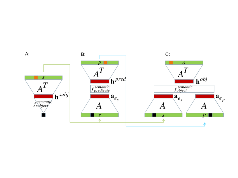
Figure 11: Semantic KG sampling using a general function approximator, e.g., a feedforward neural network. A: A subject is sampled based on $P(s)\propto\exp\beta\mathbf{a}^{\top}_{e_{s}}\mathbf{h}^{\textit{subject}}$. $\mathbf{h}^{\textit{subject}}$ is a learned latent vector. B: An predicate is sampled based on $P(p|s)\propto\exp\beta\mathbf{a}^{\top}_{e_{p}}\mathbf{h}^{\textit{predicate}}$. $\mathbf{h}^{\textit{predicate}}$ is a learned function of the sample $s$. C: An object is sampled based on $P(o|s,p)\propto\exp\beta\mathbf{a}^{\top}_{e_{o}}\mathbf{h}^{\textit{object}}$. $\mathbf{h}^{\textit{object}}$ is a learned function of the sample $s,p$.

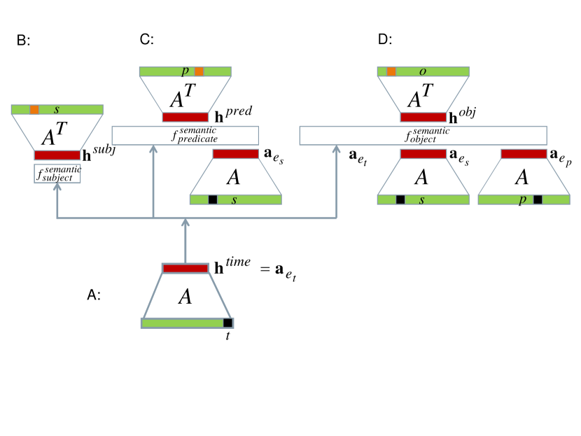
Figure 12: The semantic decoding using a general function approximator, e.g., a feedforward neural network. A: The sensory memory produces $\mathbf{h}_{t}^{\textit{time}}=\mathbf{a}_{e_{t}}$ based on $u_{:,:,t}$. $\mathbf{a}_{e_{t}}$ is represented in the weights of index neuron $e_{t}$. B: $\mathbf{a}_{e_{t}}$ is then the input to the left model and a subject $s$ is sampled based on $P(s|t)\propto\exp\beta\mathbf{a}^{\top}_{e_{s}}\mathbf{h}^{\textit{subject}}$. C: With $\mathbf{a}_{e_{t}}$ and the sampled subject as inputs, a predicate $p$ is sampled based on $P(p|s,t)\propto\exp\beta\mathbf{a}^{\top}_{e_{p}}\mathbf{h}^{\textit{predicate}}$. D: With $\mathbf{a}_{e_{t}}$ and the sampled subject and predicate as inputs, an object $o$ is sampled based on $P(o|s,p,t)\propto\exp\beta\mathbf{a}^{\top}_{e_{o}}\mathbf{h}^{\textit{object}}$.

References

- Acar et al. [2015] Evrim Acar, Rasmus Bro, and Age K Smilde. Data fusion in metabolomics using coupled matrix and tensor factorizations. Proceedings of the IEEE, 103:1602–1620, 2015.
- Airoldi et al. [2008] Edoardo M. Airoldi, David M. Blei, Stephen E. Fienberg, and Eric P. Xing. Mixed Membership Stochastic Blockmodels. Journal of Machine Learning Research, 9:1981–2014, September 2008.
- Alter et al. [2003] Orly Alter, Patrick O Brown, and David Botstein. Generalized singular value decomposition for comparative analysis of genome-scale expression data sets of two different organisms. Proceedings of the National Academy of Sciences, 100(6):3351–3356, 2003.
- Anderson [1983] John R Anderson. The architecture of cognition. Psychology Press, 1983.
- Anderson et al. [1997] John R Anderson, Michael Matessa, and Christian Lebiere. ACT-R: A theory of higher level cognition and its relation to visual attention. Human-Computer Interaction, 12(4):439–462, 1997.
- Atkinson and Shiffrin [1968] Richard C Atkinson and Richard M Shiffrin. Human memory: A proposed system and its control processes. The psychology of learning and motivation, 2:89–195, 1968.
- Auer et al. [2007] Sören Auer, Christian Bizer, Georgi Kobilarov, Jens Lehmann, Richard Cyganiak, and Zachary Ives. DBpedia: A Nucleus for a Web of Open Data. In The Semantic Web, Lecture Notes in Computer Science. Springer Berlin Heidelberg, 2007.
- Baddeley [1988] Alan Baddeley. Cognitive psychology and human memory. Trends in neurosciences, 11(4):176–181, 1988.
- Baddeley [1992] Alan Baddeley. Working memory. Science, 255(5044):556–559, 1992.
- Baddeley [2000] Alan Baddeley. The episodic buffer: a new component of working memory? Trends in cognitive sciences, 4(11):417–423, 2000.
- Baddeley [2012] Alan Baddeley. Working memory: theories, models, and controversies. Annual review of psychology, 63:1–29, 2012.
- Baddeley et al. [1974] Alan D Baddeley, Graham Hitch, et al. Working memory. The psychology of learning and motivation, 8:47–89, 1974.
- Barsalou [2009] Lawrence W Barsalou. Simulation, situated conceptualization, and prediction. Philosophical Transactions of the Royal Society of London B: Biological Sciences, 364(1521):1281–1289, 2009.
- Bartlett [1995] Frederic C Bartlett. Remembering: A study in experimental and social psychology, volume 14. Cambridge University Press, 1995.
- Barto et al. [2013] Andrew Barto, Marco Mirolli, and Gianluca Baldassarre. Novelty or surprise? Frontiers in psychology, 4, 2013.
- Becker [2005] Suzanna Becker. A computational principle for hippocampal learning and neurogenesis. Hippocampus, 15(6):722–738, 2005.
- Bengio [2012] Yoshua Bengio. Deep learning of representations for unsupervised and transfer learning. Unsupervised and Transfer Learning Challenges in Machine Learning, 7:19, 2012.
- Bengio et al. [2003] Yoshua Bengio, Réjean Ducharme, Pascal Vincent, and Christian Jauvin. A neural probabilistic language model. Journal of Machine Learning Research, 2003.
- Bengio et al. [2013] Yoshua Bengio, Aaron Courville, and Pierre Vincent. Representation learning: A review and new perspectives. Pattern Analysis and Machine Intelligence, IEEE Transactions on, 35(8):1798–1828, 2013.
- Blei et al. [2003] David M Blei, Andrew Y Ng, and Michael I Jordan. Latent dirichlet allocation. the Journal of machine Learning research, 3:993–1022, 2003.
- Bollacker et al. [2008] Kurt Bollacker, Colin Evans, Praveen Paritosh, Tim Sturge, and Jamie Taylor. Freebase: a collaboratively created graph database for structuring human knowledge. In Proceedings of the 2008 ACM SIGMOD international conference on Management of data, pages 1247–1250. ACM, 2008.
- Bordes et al. [2011] Antoine Bordes, Jason Weston, Ronan Collobert, and Yoshua Bengio. Learning structured embeddings of knowledge bases. In AAAI’11, 2011.
- Bordes et al. [2013] Antoine Bordes, Nicolas Usunier, Alberto Garcia-Duran, Jason Weston, and Oksana Yakhnenko. Translating Embeddings for Modeling Multi-relational Data. In Advances in Neural Information Processing Systems 26, 2013.
- Bourlard and Kamp [1988] Hervé Bourlard and Yves Kamp. Auto-association by multilayer perceptrons and singular value decomposition. Biological cybernetics, 59(4-5):291–294, 1988.
- Burgess and Hitch [2005] Neil Burgess and Graham Hitch. Computational models of working memory: putting long-term memory into context. Trends in cognitive sciences, 9(11):535–541, 2005.
- Cahill et al. [1995] Larry Cahill, Ralf Babinsky, Hans J Markowitsch, and James L McGaugh. The amygdala and emotional memory. Nature, 1995.
- Carlson et al. [2010] Andrew Carlson, Justin Betteridge, Bryan Kisiel, Burr Settles, Estevam R Hruschka Jr, and Tom M Mitchell. Toward an architecture for never-ending language learning. AAAI, 5:3, 2010.
- Carpenter [1989] Gail A Carpenter. Neural network models for pattern recognition and associative memory. Neural networks, 2(4):243–257, 1989.
- Clark [2013] Andy Clark. Whatever next? predictive brains, situated agents, and the future of cognitive science. Behavioral and Brain Sciences, 36(03):181–204, 2013.
- Collins and Loftus [1975] Allan M Collins and Elizabeth F Loftus. A spreading-activation theory of semantic processing. Psychological review, 82(6):407, 1975.
- Coltheart [1980] Max Coltheart. Iconic memory and visible persistence. Perception & psychophysics, 27(3):183–228, 1980.
- Conway [2009] Martin A Conway. Episodic memories. Neuropsychologia, 47(11):2305–2313, 2009.
- Conway and Pleydell-Pearce [2000] Martin A Conway and Christopher W Pleydell-Pearce. The construction of autobiographical memories in the self-memory system. Psychological review, 107(2):261, 2000.
- Cowan [1997] Nelson Cowan. Attention and memory. Oxford University Press, 1997.
- Cowan [2008] Nelson Cowan. What are the differences between long-term, short-term, and working memory? Progress in brain research, 169:323–338, 2008.
- Dayan et al. [1995] Peter Dayan, Geoffrey E Hinton, Radford M Neal, and Richard S Zemel. The helmholtz machine. Neural computation, 7(5):889–904, 1995.
- Dayan et al. [2000] Peter Dayan, Sham Kakade, and P Read Montague. Learning and selective attention. nature neuroscience, 3:1218–1223, 2000.
- Deerwester et al. [1990] Scott C. Deerwester, Susan T. Dumais, Thomas K. Landauer, George W. Furnas, and Richard A. Harshman. Indexing by latent semantic analysis. JASIS, 41(6):391–407, 1990.
- Diana et al. [2007] Rachel A Diana, Andrew P Yonelinas, and Charan Ranganath. Imaging recollection and familiarity in the medial temporal lobe: a three-component model. Trends in cognitive sciences, 11(9):379–386, 2007.
- Dong et al. [2014] Xin Dong, Evgeniy Gabrilovich, Geremy Heitz, Wilko Horn, Ni Lao, Kevin Murphy, Thomas Strohmann, Shaohua Sun, and Wei Zhang. Knowledge Vault: A Web-scale Approach to Probabilistic Knowledge Fusion. In Proceedings of the 20th ACM SIGKDD International Conference on Knowledge Discovery and Data Mining, 2014.
- Durstewitz et al. [2000] Daniel Durstewitz, Jeremy K Seamans, and Terrence J Sejnowski. Neurocomputational models of working memory. Nature neuroscience, 3:1184–1191, 2000.
- Ebbinghaus [1885] Hermann Ebbinghaus. Über das Gedächtnis: Untersuchungen zur experimentellen Psychologie. Duncker & Humblot, 1885.
- Edelman and Poggio [1992] Shimon Edelman and Tomaso Poggio. Bringing the grandmother back into the picture: A memory-based view of object recognition. International journal of pattern recognition and artificial intelligence, 6(01):37–61, 1992.
- Eichenbaum [2014] Howard Eichenbaum. Time cells in the hippocampus: a new dimension for mapping memories. Nature Reviews Neuroscience, 15(11):732–744, 2014.
- Eichenbaum et al. [2007] Howard Eichenbaum, AR Yonelinas, and Charan Ranganath. The medial temporal lobe and recognition memory. Annual review of neuroscience, 30:123, 2007.
- Eichenbaum et al. [2012] Howard Eichenbaum, Magdalena Sauvage, Norbert Fortin, Robert Komorowski, and Paul Lipton. Towards a functional organization of episodic memory in the medial temporal lobe. Neuroscience & Biobehavioral Reviews, 36(7):1597–1608, 2012.
- Ericsson and Kintsch [1995] K Anders Ericsson and Walter Kintsch. Long-term working memory. Psychological review, 102(2):211, 1995.
- Esteban et al. [2015a] Cristóbal Esteban, Danilo Schmidt, Denis Krompaß, and Volker Tresp. Predicting sequences of clinical events by using a personalized temporal latent embedding model. In Proceedings of the IEEE International Conference on Healthcare Informatics, 2015a.
- Esteban et al. [2015b] Cristóbal Esteban, Volker Tresp, Yinchong Yang, Stephan Baier, and Denis Krompaß. Predicting the co-evolution of event and knowledge graphs. arXiv preprint, 2015b.
- Frank et al. [2001] Michael J Frank, Bryan Loughry, and Randall C O’Reilly. Interactions between frontal cortex and basal ganglia in working memory: a computational model. Cognitive, Affective, & Behavioral Neuroscience, 1(2):137–160, 2001.
- Frankland and Bontempi [2005] Paul W Frankland and Bruno Bontempi. The organization of recent and remote memories. Nature Reviews Neuroscience, 6(2):119–130, 2005.
- Frankland et al. [2001] Paul W Frankland, Cara O’Brien, Masuo Ohno, Alfredo Kirkwood, and Alcino J Silva. -camkii-dependent plasticity in the cortex is required for permanent memory. Nature, 411(6835):309–313, 2001.
- Friston [2010] Karl Friston. The free-energy principle: a unified brain theory? Nature Reviews Neuroscience, 11(2):127–138, 2010.
- Gazzaniga et al. [2013] Michael S Gazzaniga, Richard B Ivry, and George Ronald Mangun. Cognitive Neuroscience: The biology of the mind. New York: WW Norton, fourth edition edition, 2013.
- George and Hawkins [2009] Dileep George and Jeff Hawkins. Towards a mathematical theory of cortical micro-circuits. PLoS Comput Biol, 5(10):e1000532, 2009.
- Gluck et al. [2003] Mark A Gluck, Martijn Meeter, and Catherine E Myers. Computational models of the hippocampal region: linking incremental learning and episodic memory. Trends in cognitive sciences, 7(6):269–276, 2003.
- Gluck et al. [2013] Mark A Gluck, Eduardo Mercado, and Catherine E Myers. Learning and memory: From brain to behavior. Palgrave Macmillan, 2013.
- Goodfellow et al. [2015] Ian Goodfellow, Aaron Courville, and Yoshua Bengio. Deep learning. Book in preparation for MIT Press, 2015.
- Gould et al. [1999] Elizabeth Gould, Alison J Reeves, Michael SA Graziano, and Charles G Gross. Neurogenesis in the neocortex of adult primates. Science, 286(5439):548–552, 1999.
- Graves et al. [2014] Alex Graves, Greg Wayne, and Ivo Danihelka. Neural turing machines. arXiv preprint arXiv:1410.5401, 2014.
- Greenberg and Verfaellie [2010] Daniel L Greenberg and Mieke Verfaellie. Interdependence of episodic and semantic memory: evidence from neuropsychology. Journal of the International Neuropsychological society, 16(05):748–753, 2010.
- Griffiths et al. [2007a] Thomas L Griffiths, Mark Steyvers, and Alana Firl. Google and the mind predicting fluency with pagerank. Psychological Science, 18(12):1069–1076, 2007a.
- Griffiths et al. [2007b] Thomas L Griffiths, Mark Steyvers, and Joshua B Tenenbaum. Topics in semantic representation. Psychological review, 114(2):211, 2007b.
- Griffiths et al. [2008] Thomas L Griffiths, Charles Kemp, and Joshua B Tenenbaum. Bayesian models of cognition. In The Cambridge Handbook of Computational Psychology. Cambridge University Press, 2008.
- Hassabis and Maguire [2007] Demis Hassabis and Eleanor A Maguire. Deconstructing episodic memory with construction. Trends in cognitive sciences, 11(7):299–306, 2007.
- Hinton [2010] Geoffrey Hinton. A practical guide to training restricted boltzmann machines. Momentum, 9(1):926, 2010.
- Hinton [1981] Geoffrey E Hinton. Implementing semantic networks in parallel hardware. In Parallel models of associative memory, pages 161–187. Erlbaum, 1981.
- Hinton and Anderson [2014] Geoffrey E Hinton and James A Anderson. Parallel Models of Associative Memory: Updated Edition. Psychology Press, 2014.
- Hinton and Salakhutdinov [2006] Geoffrey E Hinton and Ruslan R Salakhutdinov. Reducing the dimensionality of data with neural networks. Science, 313(5786):504–507, 2006.
- Hinton and Zemel [1994] Geoffrey E Hinton and Richard S Zemel. Autoencoders, minimum description length, and helmholtz free energy. Advances in neural information processing systems, pages 3–3, 1994.
- Hochreiter and Schmidhuber [1997] Sepp Hochreiter and Jürgen Schmidhuber. Long short-term memory. Neural computation, 9(8):1735–1780, 1997.
- Hofmann [1999] Thomas Hofmann. Probabilistic latent semantic indexing. In Proceedings of the 22nd annual international ACM SIGIR conference on Research and development in information retrieval, pages 50–57. ACM, 1999.
- Hopfield [1982] John J Hopfield. Neural networks and physical systems with emergent collective computational abilities. Proceedings of the national academy of sciences, 79(8):2554–2558, 1982.
- Huth et al. [2016] Alexander G. Huth, Wendy A. de Heer, Thomas L. Griffiths, Frédéric E. Theunissen, and Jack L. Gallant. Natural speech reveals the semantic maps that tile human cerebral cortex. Nature, 2016.
- Itti and Baldi [2005] Laurent Itti and Pierre F Baldi. Bayesian surprise attracts human attention. In Advances in neural information processing systems, pages 547–554, 2005.
- Jonides et al. [2008] John Jonides, Richard L Lewis, Derek Evan Nee, Cindy A Lustig, Marc G Berman, and Katherine Sledge Moore. The mind and brain of short-term memory. Annual review of psychology, 59:193, 2008.
- Karpathy and Fei-Fei [2015] Andrej Karpathy and Li Fei-Fei. Deep visual-semantic alignments for generating image descriptions. In Proceedings of the IEEE Conference on Computer Vision and Pattern Recognition, pages 3128–3137, 2015.
- Kemp et al. [2006] Charles Kemp, Joshua B. Tenenbaum, Thomas L. Griffiths, Takeshi Yamada, and Naonori Ueda. Learning systems of concepts with an infinite relational model. In Proceedings of the Twenty-First National Conference on Artificial Intelligence, volume 3 of AAAI’06, page 5, 2006.
- Kitamura et al. [2015a] Takashi Kitamura, Christopher J Macdonald, and Susumu Tonegawa. Entorhinal–hippocampal neuronal circuits bridge temporally discontiguous events. Learning & memory (Cold Spring Harbor, NY), 22(9):438–443, 2015a.
- Kitamura et al. [2015b] Takashi Kitamura, Chen Sun, Jared Martin, Lacey J Kitch, Mark J Schnitzer, and Susumu Tonegawa. Entorhinal cortical ocean cells encode specific contexts and drive context-specific fear memory. Neuron, 87(6):1317–1331, 2015b.
- Knill and Pouget [2004] David C Knill and Alexandre Pouget. The bayesian brain: the role of uncertainty in neural coding and computation. Trends in Neurosciences, 27(12):712–719, 2004.
- Kohonen [2012] Teuvo Kohonen. Self-organization and associative memory, volume 8. Springer, 2012.
- Körding et al. [2004] Konrad P Körding, Shih-pi Ku, and Daniel M Wolpert. Bayesian integration in force estimation. Journal of Neurophysiology, 92(5):3161–3165, 2004.
- Krompaß et al. [2014] Denis Krompaß, Xueyan Jiang, Maximilian Nickel, and Volker Tresp. Probabilistic Latent-Factor Database Models. In Proceedings of the 1st Workshop on Linked Data for Knowledge Discovery (ECML PKDD), 2014.
- Krompaß et al. [2015] Denis Krompaß, Stephan Baier, and Volker Tresp. Type-constrained representation learning in knowledge graphs. In The Semantic Web–ISWC 2015, pages 640–655. Springer International Publishing, 2015.
- Kumar et al. [2015] Ankit Kumar, Ozan Irsoy, Jonathan Su, James Bradbury, Robert English, Brian Pierce, Peter Ondruska, Ishaan Gulrajani, and Richard Socher. Ask me anything: Dynamic memory networks for natural language processing. arXiv preprint arXiv:1506.07285, 2015.
- Landauer and Dumais [1997] Thomas K Landauer and Susan T Dumais. A solution to plato’s problem: The latent semantic analysis theory of acquisition, induction, and representation of knowledge. Psychological review, 104(2):211, 1997.
- Landauer et al. [1998] Thomas K Landauer, Peter W Foltz, and Darrell Laham. An introduction to latent semantic analysis. Discourse processes, 25(2-3):259–284, 1998.
- Larochelle et al. [2008] Hugo Larochelle, Dumitru Erhan, and Yoshua Bengio. Zero-data learning of new tasks. AAAI, 1(2):3, 2008.
- LeCun et al. [2015] Yann LeCun, Yoshua Bengio, and Geoffrey Hinton. Deep learning. Nature, 521(7553):436–444, 2015.
- Lehn et al. [2009] Hanne Lehn, Hill-Aina Steffenach, Niels M van Strien, Dick J Veltman, Menno P Witter, and Asta K Håberg. A specific role of the human hippocampus in recall of temporal sequences. The Journal of Neuroscience, 29(11):3475–3484, 2009.
- Loftus and Ketcham [1996] Elizabeth Loftus and Katherine Ketcham. The myth of repressed memory: False memories and allegations of sexual abuse. Macmillan, 1996.
- Lund et al. [1995] Kevin Lund, Curt Burgess, and Ruth Ann Atchley. Semantic and associative priming in high-dimensional semantic space. Proceedings of the 17th annual conference of the Cognitive Science Society, 17:660–665, 1995.
- Maass [2000] Wolfgang Maass. On the computational power of winner-take-all. Neural computation, 12(11):2519–2535, 2000.
- Marr [1971] D Marr. Simple memory: A theory for archicortex. Philosophical Transactions of the Royal Society of London. Series B, Biological Sciences, pages 23–81, 1971.
- McClelland and Rumelhart [1985] James L McClelland and David E Rumelhart. Distributed memory and the representation of general and specific information. Journal of Experimental Psychology: General, 114(2):159, 1985.
- McClelland et al. [1995] James L McClelland, Bruce L McNaughton, and Randall C O’Reilly. Why there are complementary learning systems in the hippocampus and neocortex: insights from the successes and failures of connectionist models of learning and memory. Psychological review, 102(3):419, 1995.
- Morton [2013] Neal W Morton. Interactions between episodic and semantic memory. Technical report, Vanderbilt Computational Memory Lab, 2013.
- Moser et al. [2015] May-Britt Moser, David C Rowland, and Edvard I Moser. Place cells, grid cells, and memory. Cold Spring Harbor perspectives in biology, 7(2):a021808, 2015.
- Mozer [1993] Michael C Mozer. Neural net architectures for temporal sequence processing. Santa Fe Institute Studies in the Sciences of Complexity, 15:243–243, 1993.
- Ngiam et al. [2011] Jiquan Ngiam, Aditya Khosla, Mingyu Kim, Juhan Nam, Honglak Lee, and Andrew Y Ng. Multimodal deep learning. In Proceedings of the 28th international conference on machine learning (ICML-11), pages 689–696, 2011.
- Nickel [2013] Maximilian Nickel. Tensor factorization for relational learning. PhD thesis, Ludwig Maximilian University of Munich, 2013.
- Nickel and Tresp [2011] Maximilian Nickel and Volker Tresp. Learning Taxonomies from Multi-Relational Data via Hierarchical Link-Based Clustering. In Learning Semantics. Workshop at NIPS’11, Granada, Spain, 2011. URL http://learningsemanticsnips2011.wordpress.com/.
- Nickel et al. [2011] Maximilian Nickel, Volker Tresp, and Hans-Peter Kriegel. A Three-Way Model for Collective Learning on Multi-Relational Data. In Proceedings of the 28th International Conference on Machine Learning, 2011.
- Nickel et al. [2012] Maximilian Nickel, Volker Tresp, and Hans-Peter Kriegel. Factorizing YAGO: scalable machine learning for linked data. In Proceedings of the 21st International Conference on World Wide Web, WWW ’12, pages 271–280, 2012.
- Nickel et al. [2015a] Maximilian Nickel, Kevin Murphy, Volker Tresp, and Evgeniy Gabrilovich. A review of relational machine learning for knowledge graphs: From multi-relational link prediction to automated knowledge graph construction. Proceedings of the IEEE, 2015a.
- Nickel et al. [2015b] Maximilian Nickel, Lorenzo Rosasco, and Tomaso Poggio. Holographic embeddings of knowledge graphs. arXiv preprint arXiv:1510.04935, 2015b.
- O’Reilly and Frank [2006] Randall C O’Reilly and Michael J Frank. Making working memory work: a computational model of learning in the prefrontal cortex and basal ganglia. Neural computation, 18(2):283–328, 2006.
- O’Reilly et al. [1999] Randall C O’Reilly, Todd S Braver, and Jonathan D Cohen. 11 a biologically based computational model of working memory. Models of working memory: Mechanisms of active maintenance and executive control, page 375, 1999.
- Paccanaro and Hinton [2001] Alberto Paccanaro and Geoffrey E Hinton. Learning distributed representations of concepts using linear relational embedding. Knowledge and Data Engineering, IEEE Transactions on, 13(2):232–244, 2001.
- Poon and Domingos [2011] Hoifung Poon and Pedro Domingos. Sum-product networks: A new deep architecture. In Computer Vision Workshops (ICCV Workshops), 2011 IEEE International Conference on, pages 689–690. IEEE, 2011.
- Quiroga et al. [2005] R Quian Quiroga, Leila Reddy, Gabriel Kreiman, Christof Koch, and Itzhak Fried. Invariant visual representation by single neurons in the human brain. Nature, 435(7045):1102–1107, 2005.
- Quiroga [2012] Rodrigo Quian Quiroga. Concept cells: the building blocks of declarative memory functions. Nature Reviews Neuroscience, 13(8):587–597, 2012.
- Raaijmakers and Shiffrin [1981] Jeroen GW Raaijmakers and Richard M Shiffrin. SAM: A theory of probabilistic search of associative memory. The psychology of learning and motivation: Advances in research and theory, 14:207–262, 1981.
- Ranganath [2010] Charan Ranganath. Binding items and contexts the cognitive neuroscience of episodic memory. Current Directions in Psychological Science, 19(3):131–137, 2010.
- Rao and Ballard [1999] Rajesh PN Rao and Dana H Ballard. Predictive coding in the visual cortex: a functional interpretation of some extra-classical receptive-field effects. Nature neuroscience, 2(1):79–87, 1999.
- Roediger and McDermott [1995] Henry L Roediger and Kathleen B McDermott. Creating false memories: Remembering words not presented in lists. Journal of experimental psychology: Learning, Memory, and Cognition, 21(4):803, 1995.
- Rolls [2010] Edmund T Rolls. A computational theory of episodic memory formation in the hippocampus. Behavioural brain research, 215(2):180–196, 2010.
- Rolls and Deco [2010] ET Rolls and G Deco. The noisy brain. Stochastic dynamics as a principle of brain function.(Oxford Univ. Press, UK, 2010), 2010.
- Rothe and Schütze [2015] Sascha Rothe and Hinrich Schütze. Autoextend: Extending word embeddings to embeddings for synsets and lexemes. arXiv preprint arXiv:1507.01127, 2015.
- Schacter [1987] Daniel L Schacter. Implicit memory: History and current status. Journal of experimental psychology: learning, memory, and cognition, 13(3):501, 1987.
- Schacter et al. [2012] Daniel L Schacter, Donna Rose Addis, Demis Hassabis, Victoria C Martin, R Nathan Spreng, and Karl K Szpunar. The future of memory: remembering, imagining, and the brain. Neuron, 76(4):677–694, 2012.
- Schmidhuber [2009] Jürgen Schmidhuber. Driven by compression progress: A simple principle explains essential aspects of subjective beauty, novelty, surprise, interestingness, attention, curiosity, creativity, art, science, music, jokes. In Anticipatory Behavior in Adaptive Learning Systems, pages 48–76. Springer, 2009.
- Schuetze [2016] Hinrich Schuetze. Personal communication, 2016.
- Schütze [1993] Hinrich Schütze. Word space. In Advances in Neural Information Processing Systems 5. Citeseer, 1993.
- Singhal [2012] Amit Singhal. Introducing the Knowledge Graph: things, not strings, May 2012. URL http://googleblog.blogspot.com/2012/05/introducing-knowledge-graph-things-not.html.
- Smith and Kosslyn [2013] Edward E Smith and Stephen M Kosslyn. Cognitive Psychology: Pearson New International Edition: Mind and Brain. Pearson Higher Ed, 2013.
- Smolensky and Riley [1984] Paul Smolensky and Mary S Riley. Harmony theory: Problem solving, parallel cognitive models, and thermal physics. Technical report, DTIC Document, 1984.
- Socher et al. [2009] Richard Socher, Samuel Gershman, Per Sederberg, Kenneth Norman, Adler J Perotte, and David M Blei. A bayesian analysis of dynamics in free recall. In Advances in neural information processing systems, pages 1714–1722, 2009.
- Socher et al. [2013] Richard Socher, Danqi Chen, Christopher D Manning, and Andrew Ng. Reasoning With Neural Tensor Networks for Knowledge Base Completion. In Advances in Neural Information Processing Systems 26, 2013.
- Squire [1987] Larry R Squire. Memory and brain. Oxford University Press, 1987.
- Squire and Alvarez [1995] Larry R Squire and Pablo Alvarez. Retrograde amnesia and memory consolidation: a neurobiological perspective. Current opinion in neurobiology, 5(2):169–177, 1995.
- Steyvers et al. [2004] Mark Steyvers, Richard M Shiffrin, and Douglas L Nelson. Word association spaces for predicting semantic similarity effects in episodic memory. Experimental cognitive psychology and its applications: Festschrift in honor of Lyle Bourne, Walter Kintsch, and Thomas Landauer, pages 237–249, 2004.
- Suchanek et al. [2007] Fabian M. Suchanek, Gjergji Kasneci, and Gerhard Weikum. Yago: A Core of Semantic Knowledge. In Proceedings of the 16th International Conference on World Wide Web, WWW ’07. ACM, 2007.
- Sutskever et al. [2014] Ilya Sutskever, Oriol Vinyals, and Quoc V Le. Sequence to sequence learning with neural networks. In Advances in neural information processing systems, pages 3104–3112, 2014.
- Taigman et al. [2014] Yaniv Taigman, Ming Yang, Marc’Aurelio Ranzato, and Lars Wolf. Deepface: Closing the gap to human-level performance in face verification. In Computer Vision and Pattern Recognition (CVPR), 2014 IEEE Conference on, pages 1701–1708. IEEE, 2014.
- Tenenbaum et al. [2006] Joshua B Tenenbaum, Thomas L Griffiths, and Charles Kemp. Theory-based bayesian models of inductive learning and reasoning. Trends in cognitive sciences, 10(7):309–318, 2006.
- Tresp et al. [2009] Volker Tresp, Yi Huang, Markus Bundschus, and Achim Rettinger. Materializing and querying learned knowledge. Proc. of IRMLeS, 2009, 2009.
- Tulving [1972] Endel Tulving. Episodic and semantic memory 1. Organization of Memory. London: Academic, 381(e402):4, 1972.
- Tulving [1985] Endel Tulving. Elements of episodic memory. Oxford University Press, 1985.
- Tulving [2002] Endel Tulving. Episodic memory: from mind to brain. Annual review of psychology, 53(1):1–25, 2002.
- Vinyals et al. [2015] Oriol Vinyals, Alexander Toshev, Samy Bengio, and Dumitru Erhan. Show and tell: A neural image caption generator. In Proceedings of the IEEE Conference on Computer Vision and Pattern Recognition, pages 3156–3164, 2015.
- Weston et al. [2014] Jason Weston, Sumit Chopra, and Antoine Bordes. Memory networks. arXiv preprint arXiv:1410.3916, 2014.
- Wigner [1960] Eugene P Wigner. The unreasonable effectiveness of mathematics in the natural sciences. richard courant lecture in mathematical sciences delivered at new york university, may 11, 1959. Communications on pure and applied mathematics, 13(1):1–14, 1960.
- Xu et al. [2015] Kelvin Xu, Jimmy Ba, Ryan Kiros, Aaron Courville, Ruslan Salakhutdinov, Richard Zemel, and Yoshua Bengio. Show, attend and tell: Neural image caption generation with visual attention. arXiv preprint arXiv:1502.03044, 2015.
- Xu et al. [2006] Zhao Xu, Volker Tresp, Kai Yu, and Hans-Peter Kriegel. Infinite Hidden Relational Models. In Proceedings of the 22nd International Conference on Uncertainity in Artificial Intelligence, pages 544–551, 2006.
- Yang et al. [2016] Yinchong Yang, Cristóbal, and Volker Tresp. Embedding mapping approaches for tensor factorization and knowledge graph modelling. In ESWC, 2016.
- Yee et al. [2014] Eiling Yee, Evangelia G Chrysikou, and Sharon L Thompson-Schill. The Cognitive Neuroscience of Semantic Memory. Oxford Handbook of Cognitive Neuroscience, Oxford University Press, 2014.
- Zaharia et al. [2012] Matei Zaharia, Tathagata Das, Haoyuan Li, Scott Shenker, and Ion Stoica. Discretized streams: an efficient and fault-tolerant model for stream processing on large clusters. In Presented as part of the, 2012.