The Araucaria Project: High-precision orbital parallax and masses of the eclipsing binary TZ Fornacis

Abstract

Context. Independent distance estimates are particularly useful to check the precision of other distance indicators, while accurate and precise masses are necessary to constrain evolution models.

Aims. The goal is to measure the masses and distance of the detached eclipsing-binary TZ For with a precision level lower than 1 % using a fully geometrical and empirical method.

Methods. We obtained the first interferometric observations of TZ For with the VLTI/PIONIER combiner, which we combined with new and precise radial velocity measurements to derive its three-dimensional orbit, masses, and distance.

Results. The system is well resolved by PIONIER at each observing epoch, which allowed a combined fit with eleven astrometric positions. Our derived values are in a good agreement with previous work, but with an improved precision. We measured the mass of both components to be $M_{1}=2.057\pm 0.001\,M_{\odot}$ and $M_{2}=1.958\pm 0.001\,M_{\odot}$. The comparison with stellar evolution models gives an age of the system of $1.20\pm 0.10$ Gyr. We also derived the distance to the system with a precision level of 1.1 %: $d=185.9\pm 1.9$ pc. Such precise and accurate geometrical distances to eclipsing binaries provide a unique opportunity to test the absolute calibration of the surface brightness-colour relation for late-type stars, and will also provide the best opportunity to check on the future Gaia measurements for possible systematic errors.

1 Introduction

In the course of the Araucaria project, we applied different techniques for distance measurement in order to track down the influence of the population effects on the most important standard candles like Cepheids, RR Lyrae stars, red clump stars, tip of the red-giant branch (TRGB), etc. (Gieren et al. 2005a, b). Binary systems are of particular importance in our project.

Binary stars are the only tool enabling direct and accurate stellar mass measurements. This parameter is fundamental in order to understand the structure and evolution of stars, and to check the consistency with predicted values from theoretical models. In addition, such systems also provide geometrical distance measurements, which are particularly important for the cosmic distance scale. Eclipsing binary systems have the potential to provide the most accurate distance determinations to nearby galaxies with an unprecedented precision of about 1 %. Pietrzyński et al. (2013) and Graczyk et al. (2014) have already proved their efficiency by measuring the distance to the Large and Small Magellanic Cloud (LMC, SMC) with a precision of 2 % and 3 %, respectively. The approach is to fit high-quality spectroscopic and photometric observations to obtain very accurate masses, sizes, and surface brightness ratios of the components, and using a surface brightness-colour relation (SBCR, with the $V-K$ colour), the distance to the system. The results of Pietrzyński et al. (2013), who used eight eclipsing binary systems in the LMC, currently provide the best zero point for the whole extragalactic distance scale. However, the total error budget is dominated by the precision of the SBCR (about 2%). Therefore, a significant improvement on the distance determination with this technique would only be possible with a better calibration of this relation.

Another approach for measuring stellar parameters and geometrical distances with binary systems at 1 % accuracy is to combine spectroscopic and astrometric observations (see e.g. Torres et al. 2009; Zwahlen et al. 2004). This method provides a direct geometric distance and model-independent masses, and does not require any assumptions. However, the systems need to be spatially resolved to enable astrometric measurements, which is not always the case with single-dish telescope observations where the components are too close. A higher angular resolution is provided from long-baseline interferometry (LBI), where close binary systems ($<20$ mas) can be resolved. LBI already proved its efficiency in terms of angular resolution and accuracy for close binary stars (see e.g. Gallenne et al. 2015, 2014, 2013; Le Bouquin et al. 2013; Baron et al. 2012).

The nearby eclipsing binary system TZ~Fornacis (HD 20301) is an evolved double-line spectroscopic system composed of a giant (a G8III primary, $V=7.51$ mag) and a subgiant star (a F7III secondary, $V=7.76$ mag) with a 75.7-days circular orbit. Absolute parameters of this system were derived by Andersen et al. (1991) from the analysis of spectroscopic and photometric observations with an average accuracy of 2 % on the stellar parameters. Long-baseline interferometry can provide better accuracy with high-precision measurements, and is the only observing technique able to spatially resolve this system as the angular semi-major axis is $\sim 3.0$ mas. This system provides us a unique opportunity to apply both approaches to the same system, and to perform several interesting tests. In particular, comparison of the distance obtained based on spectroscopic and interferometric observations to the corresponding distance derived through the analysis of the radial velocity and photometric light curves together with a SBCR will allow the absolute calibration of the SBCR for late-type stars to be tested. Since the SBCR is the heart of accurate distance determination with eclipsing binaries to nearby galaxies, this test performed at the level of a very few percentage points is of great importance for the extragalactic distance scale.

Recently, we obtained new high-quality interferometric and spectroscopic data for this system in the course of the Araucaria project. The detailed comparison of the results from both techniques will be presented in the future once we collect the near infrared photometry. In this paper we present results from the analysis of the interferometric and spectroscopic data and compare them with the results of Andersen et al. (1991).

The spectroscopic and interferometric observations and data reduction process are presented in Sect. 2. In Sect. 3, we performed a combined fit to derive all the orbital elements, the masses, and the orbital parallax. We then discuss our results in Sect. 4 before concluding in Sect. 5.

2 Observations and data reduction

Table 1: Measured radial velocities of both components.

MJD	$V_{1}$	$e_{\mathrm{V1}}$	$V_{2}$	$e_{\mathrm{V2}}$	Instrument
	(km/s)	(km/s)	(km/s)	(km/s)
54741.186	53.83	0.03	-19.20	0.11	CORALIE
54742.184	52.47	0.03	-17.93	0.11	CORALIE
54743.161	50.89	0.03	-16.25	0.11	CORALIE
54743.187	50.85	0.03	-16.04	0.11	CORALIE
54744.092	49.20	0.03	-14.27	0.11	CORALIE
54744.169	49.03	0.03	-14.15	0.11	CORALIE
54744.384	48.62	0.03	-13.65	0.11	CORALIE
54745.111	47.11	0.03	-12.22	0.11	CORALIE
54746.115	44.88	0.03	-9.96	0.11	CORALIE
54746.233	44.61	0.03	-9.61	0.11	CORALIE
54747.182	42.28	0.03	-7.25	0.11	CORALIE
54747.290	42.01	0.03	-7.04	0.11	CORALIE
54747.392	41.73	0.03	-6.83	0.11	CORALIE
54819.102	50.38	0.03	-15.74	0.11	CORALIE
54820.110	48.48	0.03	-13.77	0.11	CORALIE
54821.093	46.41	0.03	-11.64	0.11	CORALIE
54822.117	44.05	0.03	-9.10	0.11	CORALIE
54887.047	56.78	0.03	-22.56	0.11	HARPS
55060.258	10.61	0.03	–	–	HARPS
55086.245	-9.71	0.03	47.35	0.11	CORALIE
55086.321	-9.61	0.03	47.37	0.11	CORALIE
55087.190	-7.57	0.03	45.09	0.11	CORALIE
55087.269	-7.33	0.03	45.09	0.11	CORALIE
55088.204	-4.99	0.03	42.51	0.11	CORALIE
55088.291	-4.74	0.03	42.20	0.11	CORALIE
55089.200	-2.29	0.03	–	–	CORALIE
55089.278	-2.06	0.03	39.30	0.11	CORALIE
55090.187	0.52	0.03	–	–	CORALIE
55090.258	0.70	0.03	–	–	CORALIE
55144.256	-12.15	0.03	49.89	0.11	HARPS
55431.310	33.62	0.03	–	–	HARPS
55479.107	33.59	0.03	–	–	HARPS
55499.146	52.00	0.03	-17.33	0.11	CORALIE
55500.097	50.39	0.03	-15.57	0.11	CORALIE
55501.349	48.02	0.03	-13.12	0.11	CORALIE
55504.139	41.52	0.03	-6.35	0.11	HARPS
55534.026	-19.58	0.03	57.76	0.11	HARPS
55536.020	-17.40	0.03	55.50	0.11	HARPS
56213.191	-20.72	0.03	58.96	0.11	HARPS
56213.351	-20.65	0.03	58.94	0.11	HARPS
56214.377	-20.10	0.03	58.33	0.11	HARPS
56242.019	49.20	0.03	-14.34	0.11	HARPS
56552.349	56.94	0.03	-22.64	0.11	HARPS
56577.407	-0.83	0.03	38.36	0.11	HARPS
56578.409	-3.64	0.03	41.26	0.11	HARPS
56826.423	-10.05	0.03	47.77	0.11	CORALIE
56827.420	-7.71	0.03	45.53	0.11	CORALIE
56876.440	10.05	0.03	–	–	HARPS
56877.433	6.94	0.03	–	–	HARPS
56878.440	3.87	0.03	–	–	HARPS
56879.436	0.92	0.03	–	–	HARPS
56908.315	6.96	0.03	–	–	HARPS
57005.023	56.70	0.03	-22.29	0.11	HARPS
57029.029	6.12	0.03	–	–	HARPS

2.1 New spectroscopic observations

We collected high-resolution echelle spectra from the instruments Euler/CORALIE and 3.6 m/HARPS located at La Silla Observatory (Chile). CORALIE (Queloz et al. 2001; Ségransan et al. 2010) offers a spectral resolution $R\sim 60\leavevmode\nobreak\ 000$, while we used the EGGS mode of HARPS (Mayor et al. 2003), which provided a resolution of about 80 000. Both instruments cover the spectral range $3900-6900\,\AA$. Calibrated CORALIE spectra were obtained using the Geneva pipeline, and HARPS data were processed with the standard ESO/HARPS pipeline reduction package. The average signal-to-noise ratio obtained ranges from 47 to 136 (median = 96).

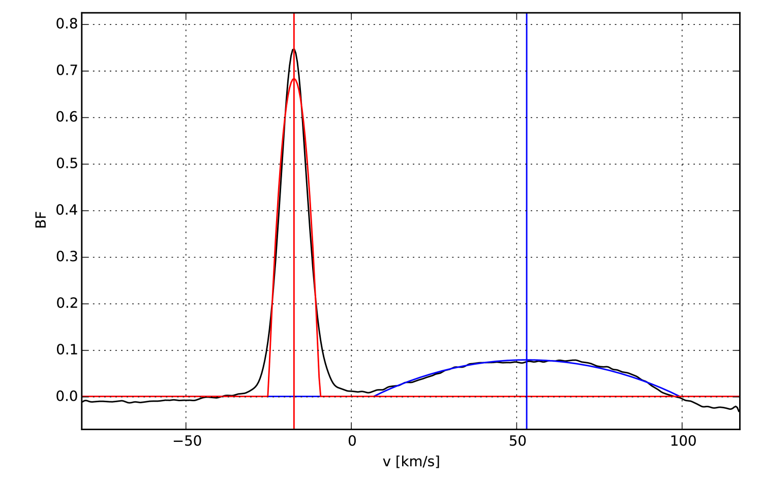
Radial velocities of both components were derived using the broadening function (BF) formalism (Rucinski 1999, 1992) implemented in the RaveSpan software (Pilecki et al. 2012). As templates we used synthetic spectra from Coelho et al. (2005) corresponding to atmospheric parameters of the TZ For components (Andersen et al. 1991). Wavelength ranges used for RV determination were: 4125–4230, 4245–4320, 4350–4840, 4880–5290, 5350–5850, 5920–6250, 6300–6420 and 6600–6840 Å. In this way we excluded troublesome hydrogen lines and most of the strong telluric lines within the 4125–6840 Å range. We derived rotational broadenings $v_{1}\sin{i}=6.1\pm 0.3\,$km s^-1 and $v_{2}\sin{i}=45.7\pm 1.0\,$km s^-1 (see Fig. 1). The BF profile of the secondary star (less massive, smaller, and hotter component) is highly rotationally broadened and the BF profiles of components are separated only in orbital quadratures.

To measure radial velocities we used two templates corresponding closely to temperature and gravity of the components. To account for line profiles blending we employed an iterative procedure. First we used the cooler template to determine velocities. We chose ten spectra uniformly distributed in orbital phase and measured the radial velocities of both components. Then we used a spectral decomposition method outlined by González & Levato (2006) to separate the spectra. A decomposed spectrum of the primary was subsequently removed from all our spectra and we determined radial velocities of the secondary, but this time we used the hotter template, fixing radial velocities of the primary. Subsequently, we repeated the spectral decomposition using all of our spectra, removing the spectrum of one component when measuring the radial velocity of the other one, each time using the appropriate template (the cooler template for the primary and the hotter for the secondary). This way we overcame the formal limitation of the BF, which allows for the use of only one radial velocity template at a time. We repeated this process three times until no progress in minimizing the dispersion of radial velocity curves was obtained. The disentangled spectra of the two stars are presented in Fig. 1. The wavelength range of the disentangled spectra is 4125–6840 Å.

The resulting velocities are presented in Table 1. In the following, we used only these radial velocities for the fitting procedure as they were derived using the same method. This will allow an independent estimate of the parameters and check for possible systematics in our results.

The orbital period $P$ and the epoch of the primary spectroscopic conjunction $T_{0}$ were estimated from the radial velocity analysis and were used for the combined fit (Sect. 3). We also detected a difference of 0.365 km s^-1 in the systemic velocity estimated from the two stars. After taking into account gravitational redshift on the surface of the components this difference is reduced to 0.208 km s^-1, but it is still significant. Although a complete study of this phenomena is beyond the scope of this paper, we note that a possible explanation can be the convective blueshift caused by cells in the atmosphere of the stars. In the case of TZ For, the giant component seems be more affected by the blueshift than its companion. This shift is taken into account in the next section by fitting two different systemic velocities.

We also checked for systematic shifts in the determination of the semi-amplitude variables $K_{1}$ and $K_{2}$. Neglecting rotational and tidal distortion in the estimates of the radial velocities produces shifts of 1.4 m s^-1 and 5.5 m s^-1, respectively for $K_{1}$ and $K_{2}$. The light time effect contribution to the semi-amplitude are 2.5 m s^-1 for both components (see Konacki et al. 2010). These values were added to the respective velocity errors for the combined fit. Amplitude of periodic relativistic effects is below 1 m s^-1 so their contribution to the radial velocities error is negligible.

From the decomposed spectra, we derived the atmospheric parameters for both stars, although less precise for the secondary because of broader lines. They were obtained using equivalent widths (EQW) of FeI line. We measured EQWs using Gaussian fitting. The strong lines showing deviation from Gaussian shape were rejected. Initial temperatures of the atmospherical models were assumed to be those typical of the spectral type of the two stars. We then refined them during the abundance analysis. As a first step, atmospherical models were calculated using ATLAS9 models (Kurucz 1970) using the initial estimates of $T_{\mathrm{eff}}$ and $v_{\mathrm{t}}=1.0\,\mathrm{km\leavevmode\nobreak\ s^{-1}}$ (turbulent velocity), and [Fe/H] = 0. The value of $T_{\mathrm{eff}}$ and $v_{\mathrm{t}}$ were then adjusted and new atmospheric models calculated in an iterative way in order to remove trends in excitation potential (EP) and equivalent width vs. abundance for $T_{\mathrm{eff}}$ and $v_{\mathrm{t}}$, respectively. The effective gravities were fixed to the values from Andersen et al. (1991) because they are better constrained. The [Fe/H] value of the models were changed at each iteration according to the output of the abundance analysis. The local thermodynamic equilibrium (LTE) program MOOG (Sneden 1973) was used for the abundance analysis. During the analysis we also rejected the lines deviating more than 3$\sigma$ from the mean [Fe/H] abundance. The derived stellar parameters are listed in Table 1. All parameters are consistent with previous work, but the effective temperature of the secondary do not have improved precision. A detailed abundance analysis will be published in a forthcoming paper about the detailed modeling of the stellar interior to calibrate convective core overshooting.

Table 2: Atmospheric parameters

	Primary	Secondary
$T_{\mathrm{eff}}$ (K)	$4930\pm 30$	$6650\pm 200$
$\log g$ (dex)	$2.91\pm 0.02$	$3.35\pm 0.02$
$v_{\mathrm{t}}$ ($\mathrm{km\leavevmode\nobreak\ s^{-1}}$)	$0.98\pm 0.10$	$3.10\pm 0.50$
$\mathrm{[Fe/H]}$ (dex)	$0.02\pm 0.05$	$-0.05\pm 0.10$

Figure 1: Left: The broadening function profiles of TZ For derived from HARPS spectrum taken on December 6, 2010. The primary rotates synchronously (high peak on left) and the secondary’s profile is flattened because of fast rotation. Right: normalized, disentangled spectra of the primary (narrow lines) and the secondary (broad shallow lines) around of H$\beta$ line.

2.2 Interferometric observations

Figure 2: Squared visibility and closure phase measurements for October 6, 2014. The data are in blue; the red dots are the fitted binary model for this epoch. The residuals are shown at the bottom.

We used the Very Large Telescope Interferometer (VLTI ; Haguenauer et al. 2010) with the four-telescope combiner PIONIER (Le Bouquin et al. 2011) to measure the squared visibilities and the closure phases. PIONIER combines the light coming from four telescopes in the $H$ band, either in a broadband mode or with a low spectral resolution, where the light is dispersed into several spectral channels. Before December 2014, the instrument allowed a spectral dispersion in three or seven channels; PIONIER was then upgraded (particularly with a grism and a new high-speed infrared detector) and now only offers dispersed fringes in six spectral channels. The recombination from all four telescopes simultaneously provides six visibility and four closure phase measurements across a range of spectral channels.

Our observations were spanned during the ESO period P94 using the 1.8 m Auxiliary Telescopes with the configuration K0-A1-G1-J3 (baselines of 57, 80, 91, 129, 132, and 140 m) and K0-A1-G1-I1 (baselines of 47, 47, 80, 90, 107, and 129 m), providing six projected baselines ranging from 40 to 140 m. A log of the observations is listed in Table 4. Data were dispersed over three or six spectral channels across the $H$ band ($1.50-1.80\,\mathrm{\mu m}$). To monitor the instrumental and atmospheric contributions, the standard observational procedure, which consists of interleaving the science target by reference stars, was used. The calibrators, listed in Table 4, were selected using the SearchCal software (Bonneau et al. 2006, 2011) provided by the Jean-Marie Mariotti Center (JMMC).

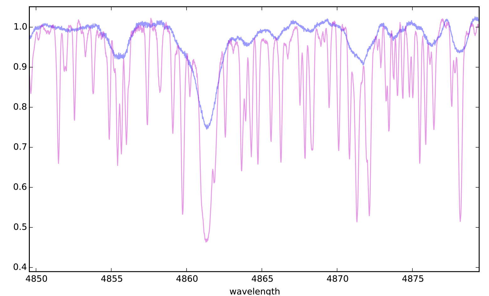
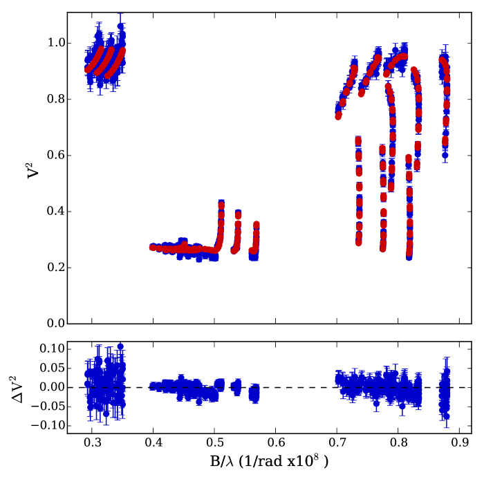
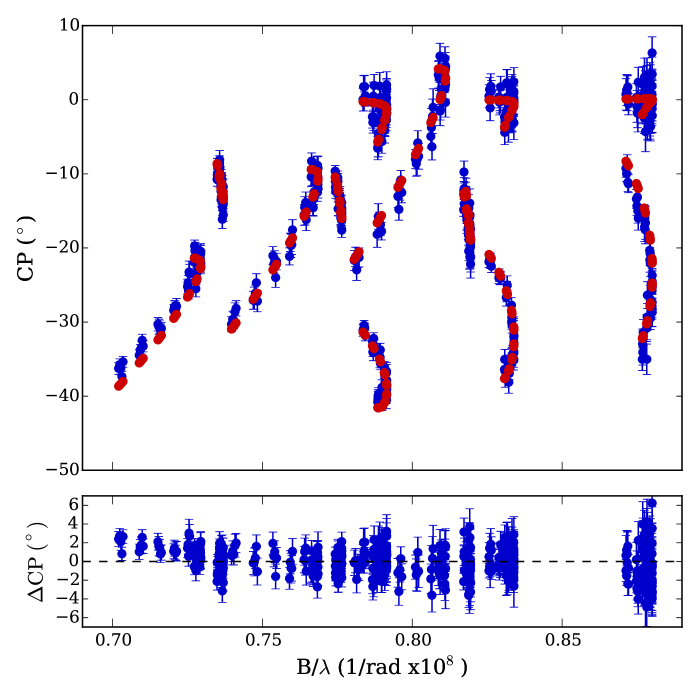
The data have been reduced with the pndrs package described in Le Bouquin et al. (2011). The main procedure is to compute squared visibilities and triple products for each baseline and spectral channel, and to correct for photon and readout noises. In Fig. 2 we present the squared visibilities and closure phases for the first observation, and where we notice that the binary nature of the system is clearly detected.

In the $H$ band, the primary star (the giant star) has an expected limb-darkened angular diameter $\theta\sim 0.42\pm 0.02$ mas (Andersen et al. 1991), whereas the secondary has an angular diameter of $0.20\pm 0.01$ mas. The primary should be spatially resolved with the larger quadruplet (K0-A1-G1-J3, with three baselines $>129$ m), while the secondary is not. We are therefore in the case of a primary resolved star plus a point source component.

For each epoch, we proceeded to a grid search to find the global minimum and the location of the companion. For this we used the interferometric tool CANDID (Gallenne et al. 2015) to search for the companion using all available observables. CANDID allows a systematic search for point-source companions performing a $N\times N$ grid of fit, whose minimum needed grid resolution is estimated a posteriori. The tool delivers the binary parameters, namely the flux ratio $f$ and the astrometric separation $(\Delta\alpha,\Delta\delta)$, but also the uniform disk angular diameter of the primary $\theta_{\mathrm{UD}}$ and the detection level of the component. For each epoch, the companion is detected at more than $50\sigma$. The final results are listed in Table 4. We estimated the uncertainties from the bootstrapping technique (with replacement) and 10 000 bootstrap samples (also included in the CANDID tool). We then took from the distributions the maximum value between the 16th and 84th percentiles as uncertainty (although the distributions were roughly symmetrical). Finally, the angular diameter was only fitted for the first three observations because we found inconsistent values with the smaller quadruplet. This is likely explained by the fact that the primary is not well resolved with this quadruplet. Its value was therefore fixed to the average value of the first three observations.

The conversion from uniform disk (UD) to limb-darkened (LD) angular diameter was done afterwards by using a linear-law parametrization $I_{\lambda}(\mu)=1-u_{\lambda}(1-\mu)$. The LD coefficient $u_{\lambda}=u_{\mathrm{H}}=0.3484$ (Claret & Bloemen 2011) was chosen taking the stellar parameters $T_{\mathrm{eff}}=5000$ K, $\log g=3.0$, [Fe/H] $=0.0$, and $v_{\mathrm{t}}=1$ km s^-1 (as close as possible to our previous derived values). The conversion is then given by the approximate formula of Hanbury Brown et al. (1974):

$$\theta_{\mathrm{LD}}(\lambda)=\theta_{\mathrm{UD}}(\lambda)\sqrt{\frac{1-u_{\lambda}/3}{1-7u_{\lambda}/15}}.$$

We estimated the mean and standard deviation of the first three observations to estimate the LD diameter $\theta_{\mathrm{LD}}=0.414\pm 0.010$ mas. It is worth mentioning that changing $v_{\mathrm{t}}$ by $\pm 2$ km s^-1 biases the LD diameter by only 0.1 % at most, which is well below our precision level.

For the $H$-band flux ratio, we took the mean value and the standard deviation between all observations to obtain $f_{\mathrm{H}}=31.8\pm 0.3$ %.

Table 3: Log of the interferometric observations together with the relative astrometric position of the second component, the flux ratio in the $H$ band and the angular diameter of the primary star.

MJD	Date	Telescope	Spectral	dof	$\Delta x$	$\Delta y$	$f$	$\theta_{\mathrm{UD}}$
		configuration	setup		(mas)	(mas)	(%)	(mas)
56937.243	2014-Oct-06	K0-A1-G1-J3	3 channels	1349	2.419$\pm$0.008	0.950$\pm$0.003	31.7$\pm$0.5	0.391$\pm$0.021
56939.234	2014-Oct-08	K0-A1-G1-J3	3 channels	1199	2.135$\pm$0.014	0.787$\pm$0.004	31.5$\pm$0.5	0.414$\pm$0.049
56962.235	2014-Oct-31	K0-A1-G1-J3	3 channels	1199	-2.346$\pm$0.005	-1.155$\pm$0.003	31.3$\pm$0.6	0.405$\pm$0.014
56979.245	2014-Nov-17	K0-A1-G1-I1	3 channels	1199	-1.801$\pm$0.004	-0.615$\pm$0.006	31.7$\pm$0.4	0.403
56995.141	2014-Dec-03	K0-A1-G1-I1	6 channels	149	1.547$\pm$0.013	0.888$\pm$0.021	32.3$\pm$0.5	0.403
56996.095	2014-Dec-04	K0-A1-G1-I1	6 channels	149	1.712$\pm$0.008	0.962$\pm$0.008	31.4$\pm$0.3	0.403
57009.062	2014-Dec-17	K0-A1-G1-I1	6 channels	2699	2.689$\pm$0.004	1.133$\pm$0.007	32.2$\pm$0.5	0.403
57011.058	2014-Dec-19	K0-A1-G1-I1	6 channels	2699	2.568$\pm$0.005	1.045$\pm$0.008	32.2$\pm$0.5	0.403
57032.088	2015-Jan-09	K0-A1-G1-I1	6 channels	2999	-1.382$\pm$0.004	-0.830$\pm$0.003	32.0$\pm$0.5	0.403
57039.099	2015-Jan-16	K0-A1-G1-I1	6 channels	2399	-2.447$\pm$0.003	-1.194$\pm$0.005	31.8$\pm$0.5	0.403
57048.078	2015-Jan-25	K0-A1-G1-I1	6 channels	2398	-2.618$\pm$0.002	-1.096$\pm$0.003	31.8$\pm$0.5	0.403

3 Orbital solutions, masses, and distance

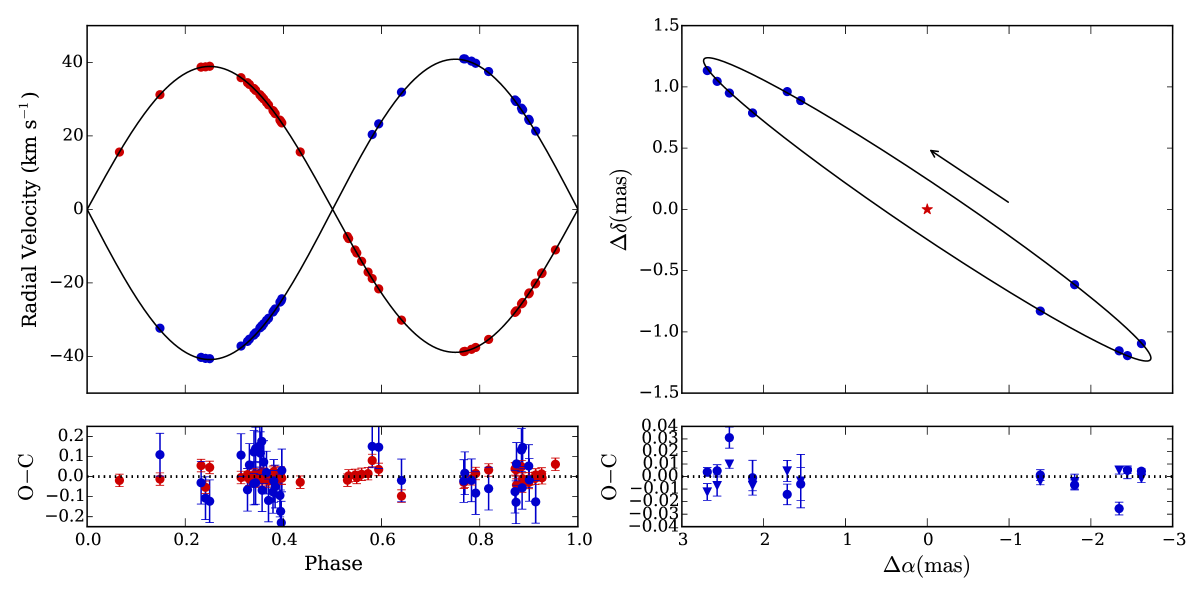
We proceeded to a combined fit of the radial velocities of both components and the astrometry of the relative orbital motion minimizing the $\chi^{2}$ using a Levenberg-Marquardt method. This provides an unambiguous determination of the masses, distance, and the orbital parameters of the system.

In a Keplerian model, the equations linking the radial velocities $V_{1}$ and $V_{2}$ to the relative projected astrometric position ($\Delta\alpha,\Delta\delta$) are (Heintz 1978)

$$\Delta\alpha = r[\sin\Omega\cos(\omega+\nu)+\cos i\cos\Omega\sin(\omega+\nu)],$$

$$\Delta\delta = r[\cos\Omega\cos(\omega+\nu)-\cos i\sin\Omega\sin(\omega+\nu)],$$

$$r = \dfrac{a(1-e^{2})}{1+e\cos\nu},$$

$$V_{1} = \gamma_{1}+K_{1}[\cos(\omega+\nu)+e\cos{\omega}],$$

$$V_{2} = \gamma_{2}-K_{2}[\cos(\omega+\nu)+e\cos{\omega}],$$

where $a$ is the angular semi-major axis, $e$ the eccentricity, $\Omega$ the longitude of ascending node, $\omega$ the argument of periastron, $i$ the orbital inclination, and $\nu$ the true anomaly estimated from the time, $P_{\mathrm{orb}}$ the orbital period, and $T_{\mathrm{p}}$ the time of the spectroscopic conjunction. The parameters $K_{1},K_{2}$ are the radial velocity amplitude of both stars, and $\gamma_{1}$ and $\gamma_{2}$ are the systemic velocities for both components. As explained in Sect 2, we detected an offset of the primary systemic velocity compared to the secondary, we therefore decided to use two different systemic velocities. We then performed a Levenberg-Marquardt fit to our data, whose fitted parameters are $P_{\mathrm{orb}},e,\omega,\Omega,i,K_{1},K_{2},\gamma_{1},\gamma_{2}$ and $a$. The final parameters are listed in Table 5. To initialize the parameters, we used the values estimated from our spectroscopic analysis and from the published values of Andersen et al. (1991). The value of $T_{0}$ was kept fixed during the fit.

From these parameters, we can derive the mass of both components and the distance to the system with (Torres et al. 2010)

$$M_{1} = \dfrac{1.036149\times 10^{-7}(K_{1}+K_{2})^{2}K_{2}P\sqrt{1-e^{2}}}{\sin^{3}i},$$

$$M_{2} = \dfrac{1.036149\times 10^{-7}(K_{1}+K_{2})^{2}K_{1}P\sqrt{1-e^{2}}}{\sin^{3}i},$$

$$a_{\mathrm{AU}} = \dfrac{9.191966\times 10^{-5}(K_{1}+K_{2})P\sqrt{1-e^{2}}}{\sin i},$$

$$d = \dfrac{a_{\mathrm{AU}}}{a}$$

where the masses are expressed in solar units, the distance in parsec, $K_{1}$ and $K_{2}$ in km s^-1, $P$ in days, and $a$ in arcsecond. The parameter $a_{\mathrm{AU}}$ is the linear semi-major axis expressed in astronomical units (the constant value of Torres et al. (2010) was converted using the astronomical constants $R_{\odot}=695.658\pm 0.140\times 10^{6}$ m from Haberreiter et al. 2008 and $AU=149\leavevmode\nobreak\ 597\leavevmode\nobreak\ 870\leavevmode\nobreak\ 700\pm 3$ m from Pitjeva & Standish 2009).

The final derived orbital elements together with the masses and the orbital parallax are listed in Table 5. The uncertainties were estimated performing 10 000 Monte Carlo simulations. We randomly created synthetic radial velocities and astrometric positions around our best fit solution and for our observing dates. We used normal distributions with standard deviations corresponding to the measurement uncertainties. We then took the median values and used the maximum value between the 16th and 84th percentiles as uncertainty estimates (although the distributions were roughly symmetrical about the median values). The systematic uncertainty from the wavelength calibration (linked to the optical path delay modulation, accurate to 1 %, Boffin et al. 2014) has to be taken into account in the angular size of the orbit (and so the distance); we therefore added in quadrature this 1 % uncertainty to the error of the semi-major axis. The final best fit orbit of TZ For is plotted in Fig. 3.

Table 4: Best fit orbital elements and parameters.

Parameter	Andersen et al. (1991)	This work
$P_{\mathrm{orb}}$ (days)	$75.6676\pm 0.0010$	$75.66647\pm 0.00006$
$T_{\mathrm{p}}$ (HJD)	$2445032.609\pm 0.002$	2452599.29040
$e$	0.0	$0.00002\pm 0.00003$
$K_{1}$ ($\mathrm{km\leavevmode\nobreak\ s^{-1}}$)	$38.81\pm 0.06$	$38.90\pm 0.01$
$K_{2}$ ($\mathrm{km\leavevmode\nobreak\ s^{-1}}$)	$40.80\pm 0.54$	$40.87\pm 0.02$
$\gamma_{1}$ ($\mathrm{km\leavevmode\nobreak\ s^{-1}}$)	$17.42\pm 0.04$	$17.99\pm 0.03$
$\gamma_{2}$ ($\mathrm{km\leavevmode\nobreak\ s^{-1}}$)	$16.30\pm 0.46$	$18.35\pm 0.11$
$\omega$ ($\degr$)	–	$269.93\pm 0.04$
$\Omega$ ($\degr$)	–	$65.99\pm 0.03$
$a$ (mas)	$2.97\pm 0.18$	$2.993\pm 0.030$
$a$ (AU)	$0.555\pm 0.004$	$0.5564\pm 0.0001$
$i$ ($\degr$)	$85.64\pm 0.05$	$85.68\pm 0.05$
$\theta_{\mathrm{LD,1}}$	$0.418\pm 0.023$	$0.414\pm 0.010$
$\theta_{\mathrm{LD,2}}$	$0.199\pm 0.012$	$0.197\pm 0.008$
$M_{1}$ ($M_{\odot}$)	$2.05\pm 0.06$	$2.057\pm 0.001$
$M_{2}$ ($M_{\odot}$)	$1.95\pm 0.03$	$1.958\pm 0.001$
$d$ (pc)	$185\pm 10$	$185.9\pm 1.9$
$\pi$ (mas)	$5.41\pm 0.29$	$5.38\pm 0.06$
$R_{1}$ ($R_{\odot}$)	$8.32\pm 0.12$	$8.28\pm 0.22$
$R_{2}$ ($R_{\odot}$)	$3.96\pm 0.09$	$3.94\pm 0.17$
$\log L_{1}/L_{\odot}$	$1.59\pm 0.04$	$1.57\pm 0.02$
$\log L_{2}/L_{\odot}$	$1.36\pm 0.03$	$1.36\pm 0.03$

Figure 3: Left: Radial velocities of the primary (red) and the secondary (blue). Right: Astrometric orbit. The triangles denote the residuals in $\Delta\delta$, while the circles denote the residuals in $\Delta\alpha$.

4 Discussion

All derived parameters are in very good agreement with the ones from Andersen et al. (1991), but we reached a better precision, especially for the masses and the distance.

From the measured flux ratio $f_{\mathrm{H}}=31.8\pm 0.3$ % and the integrated apparent magnitude of the binary $m_{\mathrm{H}}=5.129\pm 0.024$ mag (Cutri et al. 2003), we estimated an apparent magnitude of the primary and the secondary of $m_{\mathrm{H,1}}=5.429\pm 0.026$ mag and $m_{\mathrm{H,2}}=6.673\pm 0.027$ mag, respectively.

The measured angular diameter combined with our derived distance provides a consistent check of the linear radius of the primary, we found $R_{1}=8.28\pm 0.22\,R_{\odot}$, which agrees remarkably well (at a $\sim 0.2\sigma$ level) with the value derived by Andersen et al. (1991, $R_{1}=8.32\pm 0.12\,R_{\odot}$). With the radius ratio $R_{1}/R_{2}=2.10\pm 0.07$ estimated by the same authors from photometry, we also derived $R_{2}=3.94\pm 0.17\,R_{\odot}$ and $\theta_{\mathrm{LD}}=0.197\pm 0.008$ mas.

The luminosity of both components can also be obtained from

$$\dfrac{L_{\mathrm{i}}}{L_{\odot}}=\left(\dfrac{R_{\mathrm{i}}}{R_{\odot}}\right)^{2}\left(\dfrac{T_{\mathrm{eff,i}}}{T_{\odot}}\right)^{4},$$

where $\sigma$ is the Stefan–Boltzmann constant, $T_{\mathrm{eff}}$ the effective temperature, and $i=1,2$ for the components. We took $T_{\odot}=5777\pm 10$ K (Smalley 2005). The effective temperature of the primary is taken from Table 1, while the linear radii and the effective temperature of the secondary is chosen from Andersen et al. (1991) because they are more precise. The corresponding luminosities are listed in Table 5. Our value for the primary is consistent with the previous works.

Figure 4: Isochrones from the PARSEC (solid line) and BaSTI (dashed line) stellar evolution models for different metallicities, [Fe/H] = 0.02 dex (left) and 0.12 dex (right). The primary is indicated with a red dot, and the secondary in blue. The triangles denote the location of each component according to their corresponding mass.

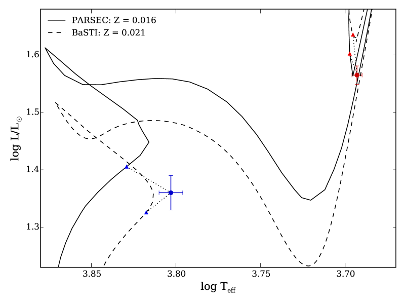
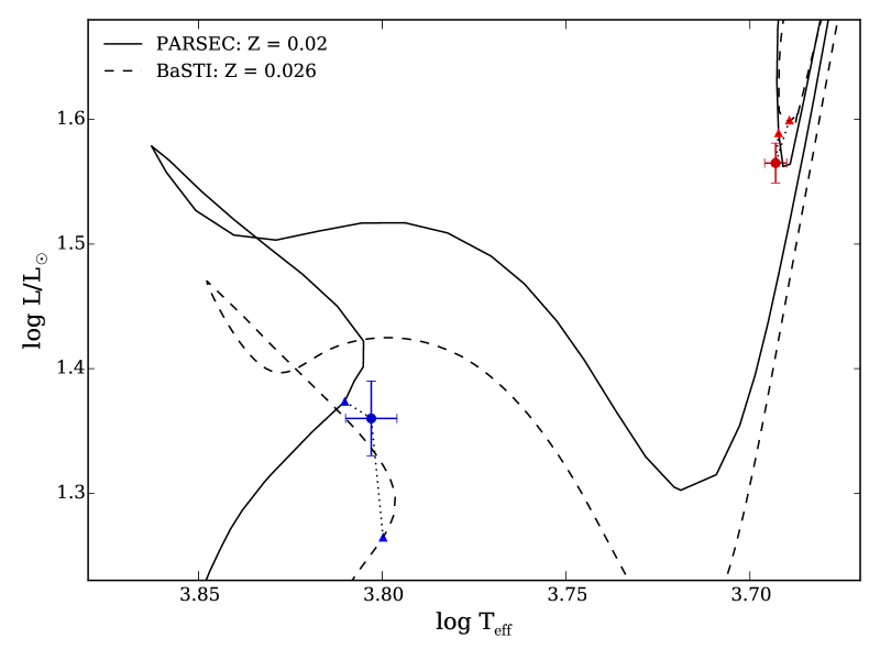
Our derived masses are also in very good agreement with Andersen et al. results. We improved the relative uncertainties on masses ($<0.1$ %), which are essential for the comparison with stellar evolution models. We checked the evolutionary status of this system using the PARSEC isochrones (Bressan et al. 2012). We fitted the age of the system according to our new [Fe/H] estimate, and allowed a single isochrone for both stars. We minimized the $\chi^{2}$ function including masses, luminosities, effective temperatures, and gravities. We used our derived masses, the effective temperature of the primary listed in Table 1, and the luminosity previously estimated, while the temperature and luminosity of the secondary are taken from Andersen et al. (1991) because they are more precise, together with the effective gravities. The value of the primary [Fe/H] = 0.02 were chosen for the models, corresponding to $Z=0.016$ for $Z_{\odot}=0.0152$ (solar metallicity used for the isochrones). We used models that include convective core overshooting with 0.25 pressure scale height above the convective border. A best fit is found for a common age $t=1.18\pm 0.03$ Gyr. We illustrate the solutions in Fig. 4. Our inferred age differs by $3.8\sigma$ from the one derived from Andersen et al. (1991, $t=1.75\pm 0.15$ Gyr), but is more consistent with Claret & Gimenez (1995, $t=1.3$ Gyr), VandenBerg et al. (2006, $t=1.12-1.33$ Gyr) and Claret (2011, $t=1.08-1.41$ Gyr). The discrepancy with Andersen’s result might be explained by the use of new opacity tables and improved stellar evolution models.

We performed a double check with the BaSTI isochrones (Pietrinferni et al. 2004), which also include convective core overshooting with 0.20 pressure scale height and scaled to a solar metallicity $Z_{\odot}=0.0198$. This translates to $Z=0.021$ for our system. We found a best fit for a common age $t=1.14\pm 0.04$ Gyr. This is consistent with the age derived from the PARSEC isochrones. The BaSTI isochrone is plotted in Fig. 4. We also note a difference in the HR diagram between the two tracks. This was already pointed out by Bressan et al. (2012). They related the different behaviour of the BaSTI tracks to the use of a different initial solar composition and their calibration to the solar model, resulting in different mixing length parameters (1.91 for BaSTI and 1.74 for PARSEC).

We tried to match the isochrones with different metallicities more closely, and we found that a metalliciy of 0.12 dex would be better for the PARSEC isochrone with a fitted age $t=1.24\pm 0.04$ Gyr, while there is no improvment with BaSTI and a fitted age $t=1.23\pm 0.04$ Gyr. Isochrones for this metallicity are shown in Fig. 4. Even if the metallicity needs to be better constrained, the age seems consistent between various models, we can therefore safely assume an average age of the system to be $t=1.20\pm 0.10$ Gyr. Although the isochrones do not perfectly match the observed position of the components, all models suggest that the primary is in the core helium buring phase. For the secondary, the models suggest that the star is around the “red hook”, i.e. at the end of its main-sequence phase, and a F7IV-V spectral is therefore more appropriate.

We provided an independent distance measurement which is compatible with the value of Andersen et al. (1991) at a 0.5 % level. Observations of such systems both by interferometry and photometry will allow the absolute calibration of the SBCR for such stars to be tested, which is of particular importance in determining precise distances ($\sim 1$ %) of nearby galaxies from eclipsing binaries (Pietrzyński et al. 2013; Graczyk et al. 2014), and therefore for the extragalactic distance scale.

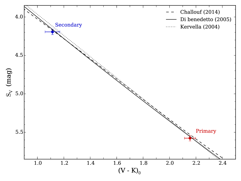
We performed a preliminary test of the existing SBCR used to predict angular diameters and distances. To this end we proceed as follows. The precise semi-major axis of the system given in Table 5 was combined with fractional radii of both components derived by Andersen et al. (1991) from light curve analysis. We obtained absolute radii $R_{1}=8.34\pm 0.11\,R_{\odot}$ and $R_{2}=3.97\pm 0.08\,R_{\odot}$. Then we built a model of the system using our Wilson-Devinney code, version 2013 (hereafter WD, Wilson & Devinney 1971), adopting a temperature of the primary component from our atmospheric analysis. The temperature of the secondary was estimated by forcing the $H$-band light ratio calculated with the WD model to be equal to direct interferometric $H$-band flux ratio. The resulting temperature was 6355 K in good agreement with the value derived by Andersen et al. (1991). We adopted the temperature of the secondary to be $6350\pm 70$ K. The slight flattening of the secondary ($\sim 1.2$ %) caused by its fast rotation was included in the model. We then used the model to calculate light ratios in Johnson $V$ and $K$ bands. The visible magnitude was taken from Andersen et al. (1991) and IR magnitude from 2MASS (Cutri et al. 2003); these values were transformed to the Johnson system using equations from Bessell & Brett (1988) and Carpenter (2001). A possible slight extinction to TZ For was pointed out previously. We calculated extinction using dust maps from Schlegel et al. (1998) with the recalibration from Schlafly & Finkbeiner (2011) to obtain $E(B-V)=0.015\pm 0.005$ mag (details of the method are given in Suchomska et al. 2015). Derredened magnitudes and angular diameters of the components were used to calculate the surface brightness $S_{\mathrm{V}}$ and intrinsic $(V-K)_{0}$ colours. Figure 5 presents both components of TZ For against three infrared SBC relations taken from the literature Challouf et al. (2014); Di Benedetto (2005); Kervella et al. (2004). Although all relations are well within observational errors, di Benedetto’s relation seems to have the most accurate slope. As di Benedetto’s relation is the one used within the Araucaria Project, we confirm here the credibility of our distances to the Magellanic Clouds of our previous works.

Figure 5: Test of the existing SBC relations using our new precise distance of TZ For.

5 Conclusions

We reported the first interferometric observations of the binary system TZ For using the VLTI/PIONIER combiner. We performed a simultaneous fit of the precise astrometric position obtained from interferometry with new radial velocity measurements. This allowed us to derive the orbital elements, the dynamical masses and the distance to the system with a precision level $<1.1$ %. The values measured for both components were $M_{1}=2.057\pm 0.001\,M_{\odot}$ and $M_{2}=1.958\pm 0.001\,M_{\odot}$. The comparison with PARSEC and BaSTI isochrones gives an average age of the system of $1.20\pm 0.10$ Gyr.

The derived distance is $d=185.9\pm 1.9$ pc, which is a precision of 1.1 %, the largest contribution to the distance uncertainty being the accuracy of the wavelength calibration (i.e 1 %). This translates to a parallax $\pi=5.379\pm 0.055$ mas. This geometrical and independent estimate of the distance can be used to check the accuracy of other distance indicators, such as the absolute calibration of the surface brightness-colour relation for late-type stars, which is the tool currently used to calibrate the first and most uncertain rungs of the cosmic distance scale using the eclipsing binary method. A preliminary test using our new precise distance of TZ For shows that the SBCR of Di Benedetto (2005) is the most consistent compared to other published relations. Other systems will be observed in the future using interferometry to check for this calibration with a larger sample.

Finally, independent and precise distance measurements of binary systems combining interferometry and spectroscopy will also provide the best opportunity to check on the future Gaia measurements for possible systematic errors.