Hydrostatic and Caustic Mass Profiles of Galaxy Clusters.

Abstract

We compare X-ray and caustic mass profiles for a sample of 16 massive galaxy clusters. We assume hydrostatic equilibrium in interpreting the X-ray data, and use large samples of cluster members with redshifts as a basis for applying the caustic technique. The hydrostatic and caustic masses agree to better than $\approx 20\%$ on average across the radial range covered by both techniques $(\sim[0.2-1.25]R_{\text{500}})$. The mass profiles were measured independently and do not assume a common functional form. Previous studies suggest that, at $R_{\text{500}}$, the hydrostatic and caustic masses are biased low and high respectively. We find that the ratio of hydrostatic to caustic mass at $R_{\text{500}}$ is $1.20^{+0.13}_{-0.11}$; thus it is larger than 0.9 at $\approx 3\sigma$ and the combination of under- and over-estimation of the mass by these two techniques is $\approx 10\%$ at most. There is no indication of any dependence of the mass ratio on the X-ray morphology of the clusters, indicating that the hydrostatic masses are not strongly systematically affected by the dynamical state of the clusters. Overall, our results favour a small value of the so-called hydrostatic bias due to non-thermal pressure sources.

1 Introduction

The observational determination of the masses of galaxy clusters is of central importance to our understanding of the growth of structure in the Universe and the use of clusters as cosmological probes. Furthermore, cluster mass is an essential reference point for studies of the astrophysical processes shaping the properties of the baryons in clusters, both the intra-cluster medium (ICM) and the member galaxies.

The task of measuring cluster masses is challenging, as their dominant dark matter component can only be studied indirectly. The total mass of a given cluster can be determined either by measuring the effect of its gravitational potential on the properties of its ICM and galaxies, or its gravitational lensing effect on the light from background sources.

The most accurate and precise mass estimation techniques include hydrostatic masses determined from X-ray observations of the ICM (Sarazin, 1986; Markevitch et al., 1998; David et al., 2001; Vikhlinin et al., 2006) caustic techniques based on galaxy dynamics (Diaferio & Geller, 1997; Rines et al., 2003, 2013; Gifford et al., 2013), and weak gravitational lensing measurements (Tyson et al., 1990; Mellier, 1999; Okabe et al., 2010; Hoekstra et al., 2015). These methods require spatially-resolved measurements with high data quality (large numbers of X-ray photons, galaxy redshifts, or lensed sources are needed). Less direct mass proxies include X-ray luminosity or temperature (e.g. Reiprich & Böhringer, 2002; Maughan, 2007; Mantz et al., 2010; Böhringer et al., 2014), and cluster richness (e.g. Rozo et al., 2008; Andreon & Hurn, 2010; Szabo et al., 2011; Rykoff et al., 2014). These lower quality mass proxies are calibrated against the more reliable measurements.

Historically, X-ray hydrostatic masses have been the gold standard for calibrating other techniques, but departures from hydrostatic equilibrium or the presence of non-thermal pressure sources (such as turbulence, bulk motions of the ICM or cosmic rays) can lead to biases in the estimated mass. Hydrodynamical simulations suggest that hydrostatic masses underestimate the true mass by $10-30\%$ (Rasia et al., 2006; Nagai et al., 2007; Lau et al., 2009; Rasia et al., 2012; Nelson et al., 2014). Observational evidence for departures from hydrostatic equilibrium has been seen for the outer parts of A1835, where the inferred hydrostatic cumulative mass profile starts to decrease un-physically with radius (Bonamente et al., 2013). In addition, uncertainties in the absolute calibration of XMM-Newton and Chandra could result in biased temperature estimates leading to biased hydrostatic mass estimates (e.g. Mahdavi et al., 2013; Rozo et al., 2014; Schellenberger et al., 2015). However, we note that Martino et al. (2014) found excellent agreement between hydrostatic masses derived from Chandra and XMM-Newton for clusters with data from both observatories.

Recently, the question of biases in hydrostatic mass estimates has received a great deal of attention as more sophisticated approaches and improved data have significantly reduced the systematic uncertainties on weak lensing masses. Several recent studies have compared weak-lensing and hydrostatic masses (sometimes indirectly through Sunyaev-Zel’dovich effect scaling relations calibrated with hydrostatic masses), finding a wide range of estimates for the amount of bias in hydrostatic masses. For example von der Linden et al. (2014b), Donahue et al. (2014), Sereno et al. (2015) and Hoekstra et al. (2015) found hydrostatic masses to be biased low by $\sim 20-30\%$, while Gruen et al. (2014), Israel et al. (2014), Applegate et al. (2016) and Smith et al. (2016) found no significant evidence for biases in the hydrostatic masses relative to weak lensing masses (with the possible exception of clusters at $z>0.3$; Smith et al., 2016, but see also Israel et al. (2014)). The underestimation of hydrostatic masses could account for some of the tension between the cosmological constraints from the Planck cosmic microwave background and cluster number counts experiments (Planck Collaboration et al., 2014a, b). At least some of the variation in estimates of the hydrostatic bias can be explained by differences in redshift range and analysis techniques used (see Smith et al., 2016), but it remains unclear at present if there is a significant bias in hydrostatic mass estimates.

Mass profile estimates from applying the caustic technique to galaxy redshift data provide an attractive alternative to weak gravitational lensing as a means of investigating biases in hydrostatic masses. The caustic method identifies the characteristic structure in the line-of-sight velocity and projected-radius space that traces the escape velocity profile of a cluster, and hence can be used to reconstruct the enclosed mass to radii well beyond the virial radius (Diaferio & Geller, 1997; Diaferio, 1999; Serra et al., 2011; Gifford et al., 2013). Like lensing measurements, caustic masses are independent of the dynamical state of the cluster, and are insensitive to the physical processes that might cause the hydrostatic biases. Caustic masses are subject to a completely different set of systematic uncertainties than lensing masses and provide a useful independent test to lensing-based studies.

Comparisons between hydrostatic and caustic mass profiles are rare, with the only previous such study limited to three clusters (Diaferio et al., 2005). Here we compare X-ray hydrostatic and caustic mass profiles for 16 massive clusters spanning a range of dynamical states. In this study, we examine the ratio of the two mass estimators as a function of cluster radius for the full sample and for subsets of relaxed and non-relaxed clusters.

The analysis assumes a WMAP9 cosmology $H_{0}=69.3{\mbox{$\text{~{}km}$}\mbox{$\text{~{}s}$}^{-1}{\mbox{$\text{~{}Mpc}$}^{-1}}\,}$, $\Omega_{m}=0.29$, $\Omega_{\Lambda}=0.71$ (Hinshaw et al., 2013).

2 Cluster Sample

We identify clusters from the Hectospec Cluster survey (HECS; Rines et al., 2013), that are also included in the complete Chandra sample of X-ray luminous clusters from Landry et al. (2013). This gives an overlap of 16 clusters, summarised in Table 1. The coordinates given in Table 1 are those of the original X-ray survey data from which the HeCS clusters were selected (Rines et al., 2013). All but one of the clusters came from the X-ray flux-limited subset of the HeCS; A2631 is a lower flux cluster that was also observed as part of the HeCS.

Table 1: The cluster sample. $N$ indicates the number of cluster members with measured redshifts for the dynamical analysis. The Chandra exposure time after cleaning of the lightcurves is given, along with the Chandra obsIDs used in the analysis. ${}^{\dagger}\text{A2631}$ is not part of the flux-limited HeCS sample.

Cluster	RA	Dec	$z$	$N$	exposure (ks)	obsID
A0267	28.1762	1.0125	0.2291	226	7	1448
A0697	130.7362	36.3625	0.2812	185	17	4217
A0773	139.4624	51.7248	0.2173	173	40	533,3588,5006
A0963	154.2600	39.0484	0.2041	211	36	903
A1423	179.3420	33.6320	0.2142	230	36	538,11724
A1682	196.7278	46.5560	0.2272	151	20	11725
A1763	203.8257	40.9970	0.2312	237	20	3591
A1835	210.2595	2.88010	0.2506	219	193	6880,6881,7370
A1914	216.5068	37.8271	0.1660	255	19	3593
A2111	234.9337	34.4156	0.2291	208	31	544,11726
A2219	250.0892	46.7058	0.2257	461	118	14355,14356,14431
A2261	260.6129	32.1338	0.2242	209	24	5007
A2631†	354.4206	0.2760	0.2765	173	26	3248,11728
RXJ1720	260.0370	26.6350	0.1604	376	45	1453,3224,4361
RXJ2129	322.4186	0.0973	0.2339	325	40	552,9370
Zw3146	155.9117	4.1865	0.2894	106	79	909,9371

3 Analysis

3.1 X-ray data

The Chandra data analysis is described in (Giles et al., 2015), which presents the X-ray scaling relations of the Landry et al. (2013) sample. The analysis closely follows that of Maughan et al. (2012), but we summarise the main steps here. The data were reduced and analysed with version 4.6 of the CIAO software package, using calibration database version 4.5.9. Projected temperature profiles of the ICM were measured from spectra extracted in annular regions centred on the X-ray centroid. Similarly, projected emissivity profiles were measured from the X-ray surface brightness in annular regions with the same centre.

Hydrostatic mass profiles $M_{\text{X}}(R)$ were derived following the method of Vikhlinin et al. (2006), assuming functional forms for the 3D density and temperature profiles of the cluster gas, and then projecting these to fit to the observed projected temperature and emissivity profiles. The best-fitting 3D profiles were then used to compute the hydrostatic mass profiles.

The statistical uncertainties on the hydrostatic mass profiles were determined with a Monte-Carlo approach (Vikhlinin et al., 2006; Giles et al., 2015). Synthetic data points were generated for the projected temperature and emissivity profiles by sampling from the best fitting models (after projection) at the radii of the original data. The samples were drawn from Gaussian distributions centred on the model value with a standard deviation given by the fractional measurement error on the original data at each point. The same fractional error was used to assign the error bar to the synthetic point.

The synthetic data were then fit in the same way as the original data, and the process was repeated 1,000 times, yielding 1,000 synthetic mass profiles. The uncertainty, $\Delta(M_{\text{X}})$, on the hydrostatic mass at any radius was then computed as

$$\frac{\Delta(M_{\text{X}})}{M_{\text{X}}}=\frac{\text{sd}(\tilde{M}_{X})}{\langle\tilde{M}_{X}\rangle}$$ (1)

where $\tilde{M}_{X}$ indicates the synthetic mass profiles, and $\text{sd}(\tilde{M}_{X})$ and $\langle\tilde{M}_{X}\rangle$ are the standard deviation and mean of the synthetic profile realisations respectively.

As described in Giles et al. (2015), clusters were also classed as relaxed, cool core clusters (hereafter RCC) if they had a low central cooling time $(<7.7\mbox{$\text{~{}Gyr}$})$, a peaked density profile (with a logarithmic slope $>0.7$ in the core), and a low centroid shift ($<0.009$, indicating regularity of X-ray isophotes). These criteria are defined and justified in Giles et al. (2015), but see also e.g. Mohr et al. (1993); Hudson et al. (2010); Maughan et al. (2012) for related discussions. This definition is fairly conservative. Only 5/16 clusters are RCC. The remaining 11 are termed NRCC, but two of these (A0963 and A2261) fail only one of the three criteria.

3.2 Galaxy caustic masses

HeCS is a spectroscopic survey of X-ray selected clusters with MMT/Hectospec (Fabricant et al., 2005). HeCS uses the caustic technique to measure mass profiles from large numbers of redshifts ($\sim 200$ members per cluster; Table 1). Galaxies in cluster infall regions occupy overdense envelopes in phase-space diagrams of line-of-sight velocity versus projected radius. The edges of these envelopes trace the escape velocity profile of the cluster and can therefore be used to determine the cluster mass profile. Diaferio & Geller (1997) show that the mass of a spherical shell within the infall region is the integral of the square of the caustic amplitude $A(r)$:

$$GM(<R)-GM(<R_{0})=\mathcal{F}_{\beta}\int_{R_{0}}^{R}A^{2}(R)\,dR$$ (2)

where $\mathcal{F}_{\beta}\simeq 0.5$ is a filling factor with a value estimated from numerical simulations (Diaferio, 1999). We approximate $\mathcal{F}_{\beta}$ as a constant; variations in $\mathcal{F}_{\beta}$ with radius lead to some systematic uncertainty in the mass profile we derive from the caustic technique. In particular, the caustic mass profile assuming constant $\mathcal{F}_{\beta}$ may overestimate the true mass profile within $\sim 0.5R_{\text{200}}$ in simulated clusters by $\sim 15\%$ or more (Serra et al., 2011). We include these issues in our assessment of the intrinsic uncertainties and biases in the technique (Serra et al., 2011). HeCS used the algorithm of Diaferio (1999) to identify the amplitude of the caustics and determine the cluster mass profiles.

The uncertainties on the caustic masses were derived from the uncertainty in the caustic location (Diaferio, 1999). Clusters like A0697 (with large uncertainties) have an irregular phase space diagram with a poorly defined edge. The clusters with small uncertainties contain large numbers of members and sharply defined edges in phase space. These errors reflect the statistical precision of the measurement; there is expected to be a $\sim 30\%$ intrinsic scatter between caustic mass and true mass (Serra et al., 2011).

3.3 Modelling the mass biases

With the mass profiles in hand, we then modelled the biases in the hydrostatic and caustic mass profiles in terms of the ratio $M_{\text{X}}/M_{\text{C}}$. Note that by convention when we report masses (i.e. in Fig. 1 and Table 2), we express them and their uncertainty as the mean ($M$) and standard deviation ($S$) of the probability distribution determined from the analyses in Sections 3.1 and 3.2 in linear space. This facilitates comparisons with other work. However, when modelling the biases in the masses the likelihood of the observed masses are assumed to be lognormal (in base 10) with mean $\mu$ and standard deviation $\sigma$. These are related to $M$ and $S$ by

$$\mu =\log_{10}\left(\frac{M}{\sqrt{1+S^{2}/M^{2}}}\right)$$ (3)

$$\sigma =\sqrt{\log_{10}\left(\frac{S^{2}}{M^{2}}+1\right)}.$$ (4)

The choice of a lognormal rather than normal distribution for the likelihood of the observed masses is motivated by the following reasons. First, the distribution of masses in the error analysis of the X-ray and caustic masses more closely resembles a lognormal than normal distribution. Second, the ratio of lognormally distributed quantities itself follows a lognormal distribution, while the ratio of normally distributed quantities follows a Cauchy distribution, which has undefined moments making the resulting uncertainty on $M_{\text{X}}/M_{\text{C}}$ harder to interpret.

In order to constrain the bias and scatter between the two mass estimators, we performed a Bayesian analysis. We constructed a model in which a given cluster has observed hydrostatic and caustic masses $\hat{\mu}_{\text{X}}$ and $\hat{\mu}_{\text{C}}$, respectively (we use $\mu$ throughout to signify logarithmic masses, and the hats indicate that these are observed quantities). These observed masses are related to the "true" hydrostatic and caustic masses $\mu_{\text{X}}$ and $\mu_{\text{C}}$ by the following stochastic relations

$$\hat{\mu}_{\text{X}}\sim\cal{N}(\mu_{\text{X}},\sigma_{\text{X}})$$ (5)

$$\hat{\mu}_{\text{C}}\sim\cal{N}(\mu_{\text{C}},\sigma_{\text{C}})$$ (6)

where "$\sim$" means "is distributed as" and $\sigma_{\text{X}}$ and $\sigma_{\text{C}}$ are the standard deviations of lognormal likelihoods describing the observed hydrostatic and caustic masses, respectively. $\cal{N}$ denotes a normal distribution. The $\hat{\mu}$ and $\sigma$ values are computed from the masses and errors given in Table 2 using Eqs 3 and 4.

These mass proxies are then related to the real mass of the cluster $\mu$ (again in base 10 log space) by the stochastic relations

$$\mu_{\text{X}}\sim\cal{N}(\mu+\kappa_{\text{X}},\delta_{\text{X}})$$ (7)

$$\mu_{\text{C}}\sim\cal{N}(\mu+\kappa_{\text{C}},\delta_{\text{C}})$$ (8)

where $\kappa_{\text{X}}$ and $\kappa_{\text{C}}$ parametrise the bias between the real mass and the hydrostatic and caustic masses, respectively. Similarly, $\delta_{\text{X}}$ and $\delta_{\text{C}}$ represent the intrinsic scatter between the real mass and the hydrostatic and caustic masses, respectively.

Weak priors were chosen for the model parameters. For each cluster, the logarithmic masses $(\mu,\mu_{\text{X}},\mu_{\text{C}})$ were assigned a uniform probability covering the range $12:17$. The logarithmic bias terms $(\kappa_{\text{X}},\kappa_{\text{C}})$ were assigned normal priors with mean 0 and standard deviation 1 (roughly speaking, we believe the mass proxies to be biased high or low by up to a factor of 10). The intrinsic scatter terms were assigned normal priors (truncated at zero) with mean $0.09$ and standard deviation $2.2$ (in natural log space this corresponds to a mean of 0.2 and standard deviation of 5; a weak prior centred on a scatter of $20\%$).

With this model, we can use our observations of $(\hat{\mu}_{\text{X}},\sigma_{\text{X}},\hat{\mu}_{\text{C}},\sigma_{\text{C}})$ for each cluster to constrain $(\kappa_{\text{X}},\delta_{\text{X}},\kappa_{\text{C}},\delta_{\text{C}})$ for the full sample. It is clear that the pairs $(\kappa_{\text{X}},\kappa_{\text{C}})$ and $(\delta_{\text{X}},\delta_{\text{C}})$ will be highly degenerate, but the mean bias between X-ray and caustic masses

$$\kappa=\kappa_{\text{X}}-\kappa_{\text{C}}=\mu_{\text{X}}-\mu_{\text{C}}=\log_{10}\left(\frac{M_{\text{X}}}{M_{\text{C}}}\right)$$ (9)

and the intrinsic scatter between X-ray and caustic masses

$$\delta=\sqrt{\delta_{\text{X}}^{2}+\delta_{\text{C}}^{2}}$$ (10)

will be constrained by the data.

The model was implemented in the probabilistic programming language Stan using the RStan interface, and the parameters were sampled with 4 chains of $5,000$ steps. This procedure was repeated using the masses measured within different radii to produce profiles of the mean bias between hydrostatic and caustic masses.

It is useful to express the mean bias $\kappa$ in terms of the mean ratio $M_{\text{X}}/M_{\text{C}}$. These are related by $\kappa=\log_{10}(M_{\text{X}}/M_{\text{C}})$. As $\kappa$ is normally distributed, the posterior distribution of $M_{\text{X}}/M_{\text{C}}$ is lognormal. We summarise this posterior of $M_{\text{X}}/M_{\text{C}}$ by quoting its median with errors given by the difference between the median and 16th and 84th percentiles. Similarly, the posterior distribution of $\delta$ is found to be approximately lognormal, so we also summarise this parameter by quoting its median with errors given by the 16th and 84th percentiles.

4 Results

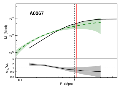
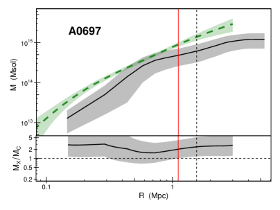
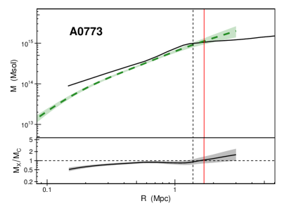
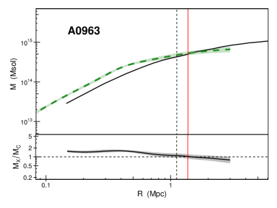
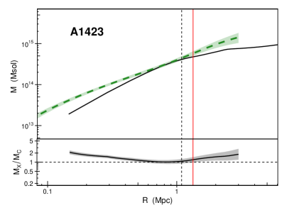
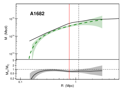
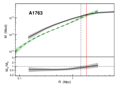
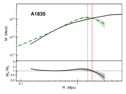
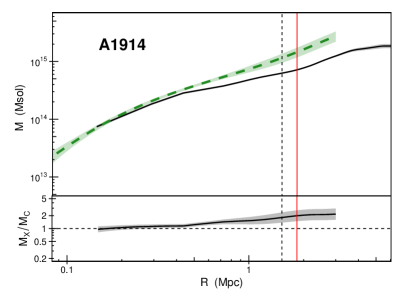
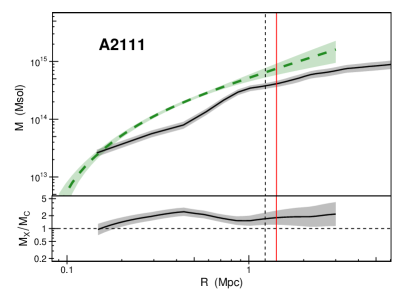
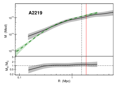
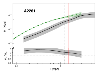
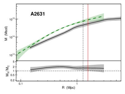
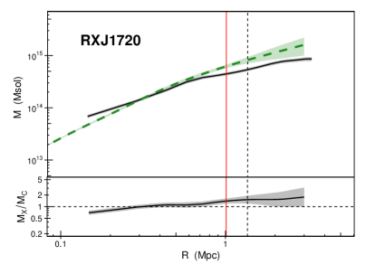
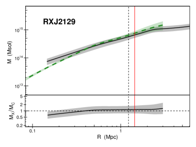
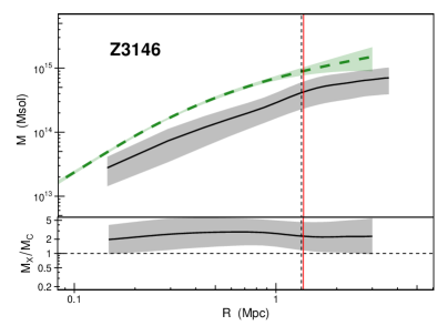
The caustic and hydrostatic cumulative mass profiles are shown for each cluster in Figs. 5 and 6 in the appendix. The hydrostatic mass profile of A1835 shows an un-physical declines at around $R_{\text{500}}$. This was first reported in Bonamente et al. (2013), and is interpreted as being due to the failure of the assumption of hydrostatic equilibrium at large radii.

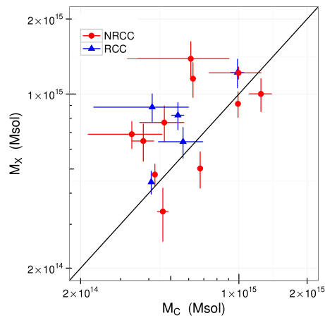
Using these profiles, the hydrostatic and caustic values of $M_{\text{500}}$ were then computed for each cluster within the radius $R_{\text{500}}$ defined from the hydrostatic mass profile. The resulting masses are compared in Fig. 1 and summarised in Table 2. For our main results we always compare quantities measured within the radius $R_{\text{500}}$ defined from the hydrostatic mass profiles. We note that this introduces a covariance between the mass measurements, but we will see below that fully consistent results are obtained when quantities are measured in a fixed aperture of $1\mbox{$\text{~{}Mpc}$}$.

Figure 1: Comparison of hydrostatic ($M_{\text{X}}$) and caustic ($M_{\text{C}}$) masses, with both measured with the radius $R_{\text{500}}$ defined from the hydrostatic mass profile. Points are coloured to indicate RCC (blue triangles) and NRCC (red circles) clusters. The solid line is the line of equality.

Cluster	z	Status	$R_{\text{500}}$	$M_{\text{X}}$	$M_{\text{C}}$
			Mpc	$10^{14}\text{M}_{\odot}$	$10^{14}\text{M}_{\odot}$
A0267	0.230	NRCC	0.99	$3.4\pm 0.8$	$4.6\pm 0.3$
A0697	0.282	NRCC	1.55	$13.9\pm 2.4$	$6.1\pm 2.9$
A0773	0.217	NRCC	1.38	$9.1\pm 1.1$	$9.9\pm 0.1$
A0963	0.206	NRCC	1.12	$4.8\pm 0.5$	$4.26\pm 0.04$
A1423	0.213	RCC	1.09	$4.4\pm 0.5$	$4.10\pm 0.07$
A1682	0.234	NRCC	1.13	$5.0\pm 0.8$	$6.74\pm 0.04$
A1763	0.223	NRCC	1.42	$10.0\pm 1.5$	$12.5\pm 1.4$
A1835	0.253	RCC	1.51	$12.2\pm 1.6$	$9.9\pm 0.7$
A1914	0.171	NRCC	1.52	$11.5\pm 1.8$	$6.3\pm 0.2$
A2111	0.229	NRCC	1.23	$6.5\pm 1.1$	$3.8\pm 0.4$
A2219	0.230	NRCC	1.52	$12.2\pm 0.7$	$10.0\pm 2.6$
A2261	0.224	NRCC	1.26	$6.9\pm 0.9$	$3.4\pm 1.2$
A2631	0.278	NRCC	1.28	$7.7\pm 1.3$	$4.7\pm 1.0$
RXJ1720	0.164	RCC	1.36	$8.2\pm 1.0$	$5.4\pm 0.3$
RXJ2129	0.235	RCC	1.22	$6.4\pm 0.9$	$5.7\pm 1.3$
Z3146	0.291	RCC	1.34	$8.9\pm 1.2$	$4.1\pm 1.9$

Table 2: Summary of the hydrostatic ($M_{\text{X}}$) and caustic ($M_{\text{C}}$) masses within the radius $R_{\text{500}}$ determined from the hydrostatic mass profile, given in column 4. The status column indicates the clusters’ dynamical classification.

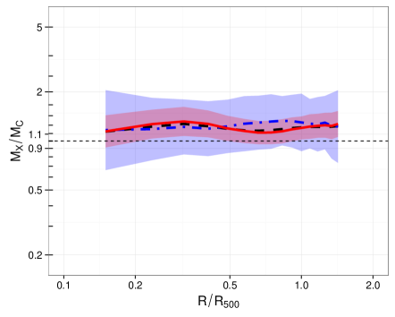
Fig. 2 shows the observed $M_{\text{X}}/M_{\text{C}}$ profile of each cluster (computed as $\hat{\mu}_{\text{X}}-\hat{\mu}_{\text{C}}$), colour-coded to indicate if a cluster is classified as RCC or NRCC. Also plotted is the profile of the mean bias $\kappa$ (expressed as $M_{\text{X}}/M_{\text{C}}$ on this logarithmic plot). The caustic and hydrostatic mass profiles agree to within $\approx 20\%$ ($\kappa\,\hbox to0.0pt{\raise 1.72218pt\hbox{$<$}\hss}{\lower 2.58334pt\hbox{$\sim$}}\,0.08$) across the radial range. In Fig. 3, the mean bias profiles of the RCC and NRCC clusters are shown separately. These profiles demonstrate a similarly good agreement between caustic and hydrostatic mass profiles for the two dynamical subsets (albeit with larger uncertainties); in both cases the agreement is better than $\approx 30\%$ ($\kappa\,\hbox to0.0pt{\raise 1.72218pt\hbox{$<$}\hss}{\lower 2.58334pt\hbox{$\sim$}}\,0.12$).

Figure 2: Profiles of the ratio of hydrostatic to caustic mass profiles for the sample. The ratios were computed in log space as described in the text. The mass profiles were scaled to the radius $R_{\text{500}}$ determined from the hydrostatic mass profile for each cluster before fitting the bias at each radius. Lines are styled to indicate RCC (blue, dot-dashed) and NRCC (red, solid) clusters. The dashed black line shows the best fitting mean bias between hydrostatic and caustic mass, with the shaded region enclosing the $1\sigma$ uncertainty.

Figure 3: Profiles of the best-fitting mean bias between hydrostatic and caustic masses. The mass profiles were scaled to the radius $R_{\text{500}}$ determined from the hydrostatic mass profile for each cluster before fitting the bias. The dashed black line shows the mean bias profile for the whole sample, while the blue (dot-dashed) and red (solid) lines with shaded error regions show the mean bias profiles for the RCC and NRCC subsets respectively.

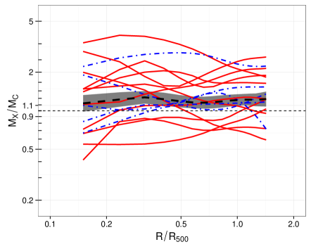
As indicated in Figs. 5 and 6, X-ray temperature profiles were measured directly close to, or beyond, $R_{\text{500}}$ for all clusters. Hydrostatic mass profiles are extrapolated based on the best-fitting temperature profile model beyond the extent of the temperature profile. The median extent of the temperature profiles is $1.25~{}R_{\text{500}}$. Profiles of the mass ratios beyond that point are less robust.

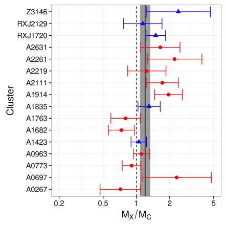
In Fig. 4, the ratio of the hydrostatic to caustic masses at the radius $R_{\text{500}}$ determined from the hydrostatic mass profile is shown for each cluster. Again, the ratios are computed as $(\hat{\mu}_{\text{X}}-\hat{\mu}_{\text{C}})$. At this radius, the two mass estimators agree well, with $\kappa=0.080\pm 0.046$, corresponding to $M_{\text{X}}/M_{\text{C}}=1.20^{+0.13}_{-0.11}$. The intrinsic scatter between the hydrostatic and caustic mass estimators at this radius is $\delta=0.11\pm 0.05\mbox{$\text{~{}dex}$}$, corresponding to an intrinsic scatter of $23^{+13}_{-10}\%$. The RCC and NRCC subsamples show consistent results, albiet with weaker constraints.

Figure 4: Ratio of hydrostatic to caustic masses at the hydrostatic $R_{\text{500}}$ for each cluster (computed as $\hat{\mu}_{\text{X}}-\hat{\mu}_{\text{C}}$). Points are coloured to indicate RCC (blue triangles) and NRCC (red circles) clusters. The solid line and shaded band shows the mean bias between the hydrostatic and caustic masses and its uncertainty.

These summary statistics are captured in Table 3, along with the same quantities derived in a fixed aperture of $1\mbox{$\text{~{}Mpc}$}$ for each cluster. The parameter values are insensitive to the choice of aperture, demonstrating that our results are not significantly influenced by scaling the caustic profiles to the hydrostatic estimate of $R_{\text{500}}$.

Table 3: Summary statistics of the ratio of the mean bias between hydrostatic and caustic masses, measured in the hydrostatic estimate of $R_{\text{500}}$ and in a fixed aperture of $1\mbox{$\text{~{}Mpc}$}$. The second column gives the subset being considered and the third column gives the mean bias. The mean bias is expressed as the mean ratio of masses in column four, and the intrinsic scatter between the mass estimators (converted to a percentage) is given in column five. Note that the quantities in columns four and five are summaries of a lognormal distribution using a median and percentiles as described in §3.3.

Aperture	Subset	$\kappa$	$M_{\text{X}}/M_{\text{C}}$	$\delta$ (%)
$R_{\text{500}}$	All	$0.080\pm 0.046$	$1.20^{+0.13}_{-0.11}$	$23^{+13}_{-10}$
$R_{\text{500}}$	RCC	$0.12\pm 0.16$	$1.31^{+0.38}_{-0.28}$	$41^{+51}_{-22}$
$R_{\text{500}}$	NRCC	$0.071\pm 0.073$	$1.17^{+0.20}_{-0.16}$	$36^{+20}_{-17}$
$1\mbox{$\text{~{}Mpc}$}$	All	$0.062\pm 0.046$	$1.15^{+0.13}_{-0.10}$	$27^{+12}_{-09}$

5 Discussion

5.1 Biases in hydrostatic and caustic masses

We have performed one of the first comparisons between mass profiles of galaxy clusters determined from their hot gas via hydrostatic assumptions, and the dynamics of their galaxies via the caustic method. These two methods are completely independent, and are subject to different assumptions and systematics. We found that, while significant scatter is present between the two estimators, the average agreement is good. As demonstrated in Fig. 2, the masses agree to better than $\approx 20\%$ on average over the full radial range sampled by both techniques. Importantly, neither of the mass measurement techniques assumed a functional form for the mass profile (although the hydrostatic analysis did use parametric temperature and density profiles). The agreement we find is not a consequence of a common parametrisation of the mass profile.

This good average agreement is somewhat surprising given that various observational and theoretical studies have suggested that hydrostatic and caustic masses are biased in opposite directions at around $R_{\text{500}}$. The caustic mass estimates make the assumption that the filling factor (a quantity related to the ratio of the mass gradient to the gravitational potential; see Serra et al., 2011, for details) is constant with radius. N-body simulations have shown this approximation breaks down in the inner parts of clusters, and that the caustic technique will tend to overestimate the true mass by $\sim 10-20\%$ at $R_{\text{500}}$, increasing to smaller radii (Serra et al., 2011). Meanwhile, hydrodynamical simulations and observational comparisons with weak lensing masses indicate that hydrostatic masses could be biased low by up to $\sim 30\%$ at $R_{\text{500}}$ due to the presence of non-thermal pressure in the gas (e.g. Lau et al., 2009; Rasia et al., 2012; Mahdavi et al., 2013; von der Linden et al., 2014b; Nelson et al., 2014).

For both caustic and hydrostatic masses, the effect of these expected biases should lead to $M_{\text{X}}/M_{\text{C}}<1$. The observed mean ratio of $1.20^{+0.13}_{-0.11}$ at $R_{\text{500}}$ places a $\sim 10\%$ upper limit (at $3\sigma$) on the combination of these two systematics (i.e. $M_{\text{X}}/M_{\text{C}}\,\hbox to0.0pt{\raise 1.72218pt\hbox{$>$}\hss}{\lower 2.58334pt\hbox{$\sim$}}\,0.9$ at $\approx 3\sigma$).

Our work provides a valuable comparison with recent studies that have attempted to constrain the level of hydrostatic bias by comparing hydrostatic and weak lensing masses. At face value there appear to be some large discrepancies, with e.g. Weighing the Giants (WtG; von der Linden et al., 2014b) and the Canadian Cluster Cosmology Project (CCCP; Hoekstra et al., 2015) finding hydrostatic masses to be biased low by $\approx 25-30\%$ at $R_{\text{500}}$, while Gruen et al. (2014), Israel et al. (2014), Applegate et al. (2016) and Smith et al. (2016) found ratios of hydrostatic to lensing mass ($M_{\text{X}}/M_{\text{WL}}$) in the range $0.92-1.06$ at $R_{\text{500}}$, which were all consistent with zero hydrostatic bias. Smith et al. (2016) limited the WtG and CCCP samples to clusters with $z<0.3$ and recomputed biases using methods consistent with their own. In this analysis the WtG and CCCP measurements became consistent with a $\,\hbox to0.0pt{\raise 1.72218pt\hbox{$<$}\hss}{\lower 2.58334pt\hbox{$\sim$}}\,10\%$ bias in the hydrostatic masses towards lower values (and consistent with zero bias). While it is not yet clear which of the different analysis methods used in these studies was optimal, the lensing-based studies appear overall to be consistent with a low or zero value of hydrostatic bias at $R_{\text{500}}$, at least for clusters at $z<0.3$.

Our measurement of $M_{\text{X}}/M_{\text{C}}=1.20^{+0.13}_{-0.11}$ provides significant support for low or zero hydrostatic bias, in a way that is independent of any systematics affecting lensing-derived masses. Further support comes from Rines et al. (2016) who compared velocity dispersions and masses derived from the Sunyaev-Zel’dovich effect (the latter calibrated from hydrostatic masses), again inferring no significant hydrostatic bias.

It is interesting to note that the agreement we found between the hydrostatic and caustic mass profiles does not appear dependent on the X-ray morphology, with the mean mass ratio profiles of the RCC and NRCC clusters in good agreement across the radial range probed (Fig. 3). Any discussion of this agreement is necessarily limited by the large uncertainties on the profiles for these subsets, but the results are suggestive that any non-thermal pressure effects are present at similar levels in the most relaxed clusters and the rest of the sample. The precision of this result is primarily limited by the small number of RCC clusters in the present sample, and will be investigated in more detail when the analysis is extended to the full flux-limited HeCS sample of 50 clusters. The inferred similarity of the hydrostatic bias for relaxed and unrelaxed clusters agrees qualitatively with the results from hydrodynamical simulations which show a fairly modest difference in the level of hydrostatic bias between relaxed and unrelaxed clusters at $R_{\text{500}}$ (e.g. Nagai et al., 2007; Lau et al., 2009).

The intrinsic scatter between the hydrostatic and caustic masses is $23^{+13}_{-10}\%$ at $R_{\text{500}}$. This is similar to the expected $\sim 30\%$ intrinsic scatter in caustic mass at a fixed true mass, caused by projection effects for non-spherical clusters (Serra et al., 2011; Gifford & Miller, 2013). These projection can thus account for all of the scatter between the mass estimators. Another possible contribution to the scatter comes from the centering of the mass profiles. Due to the hydrostatic and caustic analyses being performed independently, their profiles were not centred on the same coordinates. For each cluster, the X-ray profiles were centred on the centroid of the X-ray emission, while the caustic profiles were centred on the hierarchical centre of the galaxy distribution. This difference in central position should not affect the average agreement between the mass profiles, but will contribute to the intrinsic scatter between the masses.

5.2 Possible systematic effects

For our main results, we scaled the caustic mass profiles to the hydrostatic estimate of $R_{\text{500}}$. Such scaling is useful, since $R_{\text{500}}$ is a commonly-used reference radius for mass comparisons, but it introduces covariance between the masses. This could suppress scatter between the two estimators. We verified that the use of the hydrostatic $R_{\text{500}}$ did not significantly influence our results by repeating the analysis using unscaled profiles and comparing the masses at $1\mbox{$\text{~{}Mpc}$}$. As shown in Table 3 the results were insensitive to the choice of radius, and the average agreement between the two mass estimators remained good.

An additional systematic that can effect the hydrostatic masses is the calibration of the X-ray observatories. It is well known that Chandra and XMM-Newton show systematic differences in temperatures measured for hot clusters. Recently, Schellenberger et al. (2015) showed that hydrostatic masses are on average $14\%$ lower when inferred from XMM-Newton observations than from Chandra (but see Martino et al., 2014). Thus, if we scaled our Chandra hydrostatic masses to the XMM-Newton calibration, our inferred $M_{\text{X}}/M_{\text{C}}$ would reduce to $1.05$, more easily accommodating a larger hydrostatic bias as inferred from some weak lensing comparisons and/or the expected systematic overestimate of the caustic masses at $R_{\text{500}}$. However, it is by no means clear that this is the correct approach. Firstly, the three imaging detectors on XMM-Newton do not measure consistent temperatures with each-other (Schellenberger et al., 2015). Secondly, calibrating the XMM-Newton derived hydrostatic mass scale used by Planck Collaboration et al. (2014b) to the higher Chandra masses helps reduce the tension between the cosmological parameters inferred from the Planck cluster counts and the cosmic microwave background (Schellenberger et al., 2015). It is clear that the X-ray calibration is a significant systematic uncertainty affecting the interpretation of our results.

5.3 Direct comparisons of our masses with other work

In this section we directly compare the masses measured for the clusters in our sample with those from other work.

We compared our hydrostatic masses with those measured by other authors using Chandra observations of the same clusters. All of the clusters in our sample were analysed by Martino et al. (2014), and nine were in the sample of Mahdavi et al. (2013). In both cases we remeasured our hydrostatic masses within the same $R_{\text{500}}$ radii used in the comparison study, to ensure consistency. The weighted mean ratio of our hydrostatic masses to those of Martino et al. (2014) was $1.05\pm 0.07$, and to those of Mahdavi et al. (2013) was $1.04\pm 0.09$; a very good agreement in both cases. We can thus conclude that the measured $M_{\text{X}}/M_{\text{C}}$ is unlikely to be overestimated due to systematics in the X-ray analysis.

Many of the clusters in our sample have been studied by one or more weak-lensing project (e.g. Okabe & Smith, 2016; von der Linden et al., 2014a; Hoekstra et al., 2015; Merten et al., 2015). In Geller et al. (2013), mass profiles from caustics and weak lensing were compared for 19 clusters (17 from HeCS, with lensing masses from various sources). Caustic masses were found to be larger than lensing masses at radii smaller than $R_{\text{200}}$, and in good agreement around $R_{\text{200}}$. Since that comparison was made, however, many of the lensing masses that were used have been revised upwards following updated analyses (Okabe & Smith, 2016; Hoekstra et al., 2015). Hoekstra et al. (2015) compared caustic and lensing masses within $R_{\text{200}}$ for 14 clusters in common between their lensing sample and the HeCS. They found a mean ratio of lensing to caustic masses of $M_{\text{WL}}/M_{\text{C}}=1.22\pm 0.07$. The difference from the good agreement found at $R_{\text{200}}$ by Geller et al. (2013) is at least partly due to the revision upwards of the lensing masses in Hoekstra et al. (2015) compared to those used in Geller et al. (2013). Also, two of the clusters in the comparison sample contain multiple clusters along the line of sight. Because weak lensing measures the total mass of all systems while the caustic technique measures the mass of the largest cluster, these mass estimates are significant outliers and may bias the mean ratio (Geller et al., 2013; Hoekstra et al., 2015).

A full comparison of our caustic and hydrostatic masses with the range of new and updated lensing masses requires a careful comparison of mass profiles on a cluster-by-cluster basis taking into account contamination by foreground structures (e.g. Hwang et al., 2014). This is beyond the scope of the current paper. For the present, we performed a simple comparison of our caustic and hydrostatic masses with the lensing masses of Hoekstra et al. (2015) for nine clusters in common between the samples (the Hoekstra et al., 2015, dataset was chosen for this simple comparison as it is recent and has the largest overlap with our current sample from a single lensing study). For this comparison, we used the NFW $M_{\text{500}}$ masses from Hoekstra et al. (2015), and recomputed the hydrostatic and caustic masses within the radius $R_{\text{500}}$ measured from the weak lensing data. We found that both the X-ray and caustic masses were consistent, on average, with the lensing masses, though the small number of clusters available limited the precision of the comparison.

6 Summary

For 16 massive clusters, we compared the hydrostatic and caustic masses based, respectively, on X-ray and optical data. We conclude:

• The hydrostatic and caustic masses agree to better than $\approx 20\%$ on average across the radial range covered by both techniques. The mass profiles were measured independently and the agreement in masses not due to a shared parametrisation of the mass profiles.

• The ratio $M_{\text{X}}/M_{\text{C}}\,\hbox to0.0pt{\raise 1.72218pt\hbox{$>$}\hss}{\lower 2.58334pt\hbox{$\sim$}}\,0.9$ at $R_{\text{500}}$ (at $3\sigma$), placing a limit on the amount by which hydrostatic masses are underestimated or caustic masses are overestimated. Our results favour a low (or zero) value of hydrostatic bias, consistent with some of the recent lensing-based estimates.

• There is no indication of any dependence of $M_{\text{X}}/M_{\text{C}}$ on the X-ray morphology of the clusters although the comparison is currently limited by the small sample size, indicating that the hydrostatic masses are not strongly systematically affected by the dynamical state of the clusters.

• The scatter between $M_{\text{X}}$ and $M_{\text{C}}$ is $23^{+13}_{-10}\%$ at $R_{\text{500}}$, and is consistent with being due to the expected scatter in caustic mass from projection effects.

We plan to use new Chandra observations to extend this analysis to the complete flux-limited sample of 50 HeCS clusters.

Appendix A Mass profile plots

Figures 5 and 6 show the hydrostatic and caustic mass profiles for each cluster in our sample.

Figure 5: The upper panels in each plot show the caustic (black solid) and hydrostatic (green dashed) mass profiles for each cluster, while the lower panels show the ratio of the hydrostatic to caustic masses. The shaded regions indicate $1\sigma$ uncertainties. The vertical black dashed line indicates the value of $R_{\text{500}}$ estimated from the hydrostatic profile, and the vertical red solid line indicates the extent of the measured temperature profile - hydrostatic masses beyond this radius are based on extrapolation.

Figure 6: The upper panels in each plot show the caustic (black solid) and hydrostatic (green dashed) mass profiles for each cluster, while the lower panels show the ratio of the hydrostatic to caustic masses. The shaded regions indicate $1\sigma$ uncertainties. The vertical black dashed line indicates the value of $R_{\text{500}}$ estimated from the hydrostatic profile, and the vertical red solid line indicates the extent of the measured temperature profile - hydrostatic masses beyond this radius are based on extrapolation.

References

- Andreon & Hurn (2010) Andreon S., Hurn M. A., 2010, MNRAS, 404, 1922
- Applegate et al. (2016) Applegate D. E., et al., 2016, MNRAS, 457, 1522
- Böhringer et al. (2014) Böhringer H., Chon G., Collins C. A., 2014, A&A, 570, A31
- Bonamente et al. (2013) Bonamente M., Landry D., Maughan B., Giles P., Joy M., Nevalainen J., 2013, MNRAS, 428, 2812
- David et al. (2001) David L. P., Nulsen P. E. J., McNamara B. R., Forman W., Jones C., Ponman T., Robertson B., Wise M., 2001, ApJ, 557, 546
- Diaferio (1999) Diaferio A., 1999, MNRAS, 309, 610
- Diaferio & Geller (1997) Diaferio A., Geller M. J., 1997, ApJ, 481, 633
- Diaferio et al. (2005) Diaferio A., Geller M. J., Rines K. J., 2005, ApJ, 628, L97
- Donahue et al. (2014) Donahue M., et al., 2014, ApJ, 794, 136
- Fabricant et al. (2005) Fabricant D., et al., 2005, PASP, 117, 1411
- Geller et al. (2013) Geller M. J., Diaferio A., Rines K. J., Serra A. L., 2013, ApJ, 764, 58
- Gifford & Miller (2013) Gifford D., Miller C. J., 2013, ApJ, 768, L32
- Gifford et al. (2013) Gifford D., Miller C., Kern N., 2013, ApJ, 773, 116
- Giles et al. (2015) Giles P. A., et al., 2015, astro-ph/1510.04270
- Gruen et al. (2014) Gruen D., et al., 2014, MNRAS, 442, 1507
- Hinshaw et al. (2013) Hinshaw G., et al., 2013, ApJS, 208, 19
- Hoekstra et al. (2015) Hoekstra H., Herbonnet R., Muzzin A., Babul A., Mahdavi A., Viola M., Cacciato M., 2015, MNRAS, 449, 685
- Hudson et al. (2010) Hudson D. S., Mittal R., Reiprich T. H., Nulsen P. E. J., Andernach H., Sarazin C. L., 2010, A&A, 513, A37+
- Hwang et al. (2014) Hwang H. S., Geller M. J., Diaferio A., Rines K. J., Zahid H. J., 2014, ApJ, 797, 106
- Israel et al. (2014) Israel H., Reiprich T. H., Erben T., Massey R. J., Sarazin C. L., Schneider P., Vikhlinin A., 2014, A&A, 564, A129
- Landry et al. (2013) Landry D., Bonamente M., Giles P., Maughan B., Joy M., Murray S., 2013, MNRAS, 433, 2790
- Lau et al. (2009) Lau E. T., Kravtsov A. V., Nagai D., 2009, ApJ, 705, 1129
- Mahdavi et al. (2013) Mahdavi A., Hoekstra H., Babul A., Bildfell C., Jeltema T., Henry J. P., 2013, ApJ, 767, 116
- Mantz et al. (2010) Mantz A., Allen S. W., Rapetti D., Ebeling H., 2010, MNRAS, 406, 1759
- Markevitch et al. (1998) Markevitch M., Forman W. R., Sarazin C. L., Vikhlinin A., 1998, ApJ, 503, 77
- Martino et al. (2014) Martino R., Mazzotta P., Bourdin H., Smith G. P., Bartalucci I., Marrone D. P., Finoguenov A., Okabe N., 2014, MNRAS, 443, 2342
- Maughan (2007) Maughan B. J., 2007, ApJ, 668, 772
- Maughan et al. (2012) Maughan B. J., Giles P. A., Randall S. W., Jones C., Forman W. R., 2012, MNRAS, 421, 1583
- Mellier (1999) Mellier Y., 1999, ARA&A, 37, 127
- Merten et al. (2015) Merten J., et al., 2015, ApJ, 806, 4
- Mohr et al. (1993) Mohr J. J., Fabricant D. G., Geller M. J., 1993, ApJ, 413, 492
- Nagai et al. (2007) Nagai D., Vikhlinin A., Kravtsov A. V., 2007, ApJ, 655, 98
- Nelson et al. (2014) Nelson K., Lau E. T., Nagai D., 2014, ApJ, 792, 25
- Okabe & Smith (2016) Okabe N., Smith G. P., 2016, MNRAS, 461, 3794
- Okabe et al. (2010) Okabe N., Takada M., Umetsu K., Futamase T., Smith G. P., 2010, PASJ, 62, 811
- Planck Collaboration et al. (2014a) Planck Collaboration et al., 2014a, A&A, 571, A16
- Planck Collaboration et al. (2014b) Planck Collaboration et al., 2014b, A&A, 571, A20
- Rasia et al. (2006) Rasia E., et al., 2006, MNRAS, 369, 2013
- Rasia et al. (2012) Rasia E., et al., 2012, New Journal of Physics, 14, 055018
- Reiprich & Böhringer (2002) Reiprich T. H., Böhringer H., 2002, ApJ, 567, 716
- Rines et al. (2003) Rines K., Geller M. J., Kurtz M. J., Diaferio A., 2003, AJ, 126, 2152
- Rines et al. (2013) Rines K., Geller M. J., Diaferio A., Kurtz M. J., 2013, ApJ, 767, 15
- Rines et al. (2016) Rines K. J., Geller M. J., Diaferio A., Hwang H. S., 2016, ApJ, 819, 63
- Rozo et al. (2008) Rozo E., et al., 2008, astro-ph/0809.2797
- Rozo et al. (2014) Rozo E., Rykoff E. S., Bartlett J. G., Evrard A., 2014, MNRAS, 438, 49
- Rykoff et al. (2014) Rykoff E. S., et al., 2014, ApJ, 785, 104
- Sarazin (1986) Sarazin C. L., 1986, Reviews of Modern Physics, 58, 1
- Schellenberger et al. (2015) Schellenberger G., Reiprich T. H., Lovisari L., Nevalainen J., David L., 2015, A&A, 575, A30
- Sereno et al. (2015) Sereno M., Ettori S., Moscardini L., 2015, MNRAS, 450, 3649
- Serra et al. (2011) Serra A. L., Diaferio A., Murante G., Borgani S., 2011, MNRAS, 412, 800
- Smith et al. (2016) Smith G. P., et al., 2016, MNRAS, 456, L74
- Szabo et al. (2011) Szabo T., Pierpaoli E., Dong F., Pipino A., Gunn J., 2011, ApJ, 736, 21
- Tyson et al. (1990) Tyson J. A., Wenk R. A., Valdes F., 1990, ApJ, 349, L1
- Vikhlinin et al. (2006) Vikhlinin A., Kravtsov A., Forman W., Jones C., Markevitch M., Murray S. S., Van Speybroeck L., 2006, ApJ, 640, 691
- von der Linden et al. (2014a) von der Linden A., et al., 2014a, MNRAS, 439, 2
- von der Linden et al. (2014b) von der Linden A., et al., 2014b, MNRAS, 443, 1973