Progenitor-dependent Explosion Dynamics in Self-consistent, Axisymmetric Simulations
of Neutrino-driven Core-collapse Supernovae

Abstract

We present self-consistent, axisymmetric core-collapse supernova simulations performed with the Prometheus-Vertex code for 18 pre-supernova models in the range of 11–28 $\mathrm{M}_{\odot}$, including progenitors recently investigated by other groups. All models develop explosions, but depending on the progenitor structure, they can be divided into two classes. With a steep density decline at the Si/Si-O interface, the arrival of this interface at the shock front leads to a sudden drop of the mass-accretion rate, triggering a rapid approach to explosion. With a more gradually decreasing accretion rate, it takes longer for the neutrino heating to overcome the accretion ram pressure and explosions set in later. Early explosions are facilitated by high mass-accretion rates after bounce and correspondingly high neutrino luminosities combined with a pronounced drop of the accretion rate and ram pressure at the Si/Si-O interface. Because of rapidly shrinking neutron star radii and receding shock fronts after the passage through their maxima, our models exhibit short advection time scales, which favor the efficient growth of the standing accretion-shock instability. The latter plays a supportive role at least for the initiation of the re-expansion of the stalled shock before runaway. Taking into account the effects of turbulent pressure in the gain layer, we derive a generalized condition for the critical neutrino luminosity that captures the explosion behavior of all models very well. We validate the robustness of our findings by testing the influence of stochasticity, numerical resolution, and approximations in some aspects of the microphysics.

1. Introduction

Nearly half a century after the first suggestion (Colgate & White, 1966) that neutrinos might play an important role in core-collapse supernovae (CCSNe), the viability of the delayed neutrino-driven mechanism (Bethe & Wilson, 1985) is still controversially discussed. Although the degree of sophistication of the explosion models has continuously increased and a growing number of multidimensional simulations have been conducted over the past years, the conclusions with respect to the neutrino-driven mechanism are contradictive and an unambiguous verification of the physics that drives the explosion has not yet been possible.

While successful explosions with simulations in spherical symmetry (1D) including state-of-the-art physics could only be obtained in cases of stars with O-Ne-Mg and low-mass Fe cores (Kitaura et al., 2006; Janka et al., 2008; Fischer et al., 2010; Melson et al., 2015b), explosion models in two dimensions (i.e. with assumed axisymmetry; 2D) demonstrated the important and supportive role of multidimensional effects. However, the 2D results reported by various groups differ considerably. According to the results by, for example, Marek & Janka (2009), Janka et al. (2012), Suwa et al. (2010, 2016), Nakamura et al. (2015), Müller et al. (2012a, b), and Müller & Janka (2014), simulations in axisymmetry show rather late explosions with energies seemingly below the canonical value of $10^{51}\,\mathrm{erg}$ for typical CCSNe. Of course, it has to be noted that not all simulations were continued to the time when a saturation of the explosion energy can be expected. Bruenn et al. (2013, 2016) presented four 2D simulations for progenitors with zero-age main sequence (ZAMS) masses between 12 M_⊙ and 25 M_⊙ where the explosions already begin at fairly early times after bounce ($\sim 0.2$ s) and the explosion energies are in reach of those deduced from observations. Curiously, in spite of the different structures of the four progenitor models, all explosions (i.e. runaway shock expansions) set in nearly at the same time. Using the same four progenitor models, but different treatments concerning hydrodynamics, gravity, equation of state (EoS), and neutrino transport, Dolence et al. (2015) did not find any explosion, while Skinner et al. (2015) and O’Connor & Couch (2015) reported failures or successes that depended on the applied gravity (Newtonian or relativistic potential) and transport treatment (for a summary of recent 2D results, the reader is also referred to Janka et al., 2016). This unsatisfactory situation clearly underlines the need for more detailed tests and code comparisons among the different CCSN simulation groups in the future.

The imposed symmetry constraints in 2D simulations are also the cause of drawbacks. The unipolar or bipolar deformations along the symmetry axis observed in 2D models seem to be strongly connected to the artificial assumption of rotational symmetry, and the inverse turbulent energy cascade distributes the energy in an unphysical way to the largest scales (see Kraichnan, 1967; Hanke et al., 2012; Couch, 2013; Radice et al., 2016). But due to the huge computational demands of self-consistent simulations in three dimensions (see e.g. Hanke et al., 2013; Tamborra et al., 2013, 2014b, 2014a; Takiwaki et al., 2014; Melson et al., 2015b, a; Müller, 2015; Lentz et al., 2015; Kuroda et al., 2012, 2016), systematic studies of larger sets of progenitor models or detailed investigations of different explosion parameters are restricted to the axisymmetric modeling approach at the moment. Even in 2D, investigations of a wider range of pre-supernova models usually employ only simplified neutrino transport schemes (e.g., Nakamura et al., 2015; Pan et al., 2016; Suwa et al., 2016).

In the following, we report the results of 2D simulations with the Prometheus-Vertex code from Hanke (2014). The consideration of a large set of 18 different pre-supernova models allows us to investigate the influence of the progenitor structure on the explosion physics in a systematic way, and a connection of progenitor properties to certain aspects of the evolution of the supernova explosion becomes possible. Besides a set of 14 pre-supernova models from Woosley et al. (2002), we include the four progenitors from Woosley & Heger (2007) that were chosen by Bruenn et al. (2013, 2016), Dolence et al. (2015), O’Connor & Couch (2015), and Skinner et al. (2015) and discuss our simulation results of these four models in depth. This is intended to facilitate future comparisons between the different simulation groups and will hopefully help to shed light on the currently rather diffuse situation regarding the outcomes of CCSN simulations with different codes.

Motivated by the question why the explosions in our models set in at largely different times without any obvious connection to special values of individual parameters like the non-radial kinetic energy, heating efficiency or maximum/average entropy in the gain layer, we will also present a theoretical analysis that sets our results into the context of the critical luminosity concept for the initiation of neutrino-driven explosions. We will show that the critical condition of $L_{\nu}\langle E_{\nu}^{2}\rangle$ as a function of $\dot{M}M_{\mathrm{NS}}$ coined by Müller & Janka (2015) ($L_{\nu}$ denotes the total electron-flavor neutrino luminosity, $\langle E_{\nu}^{2}\rangle$ the weighted average of the mean squared energies of electron neutrinos and antineutrinos, $\dot{M}$ the mass-accretion rate, and $M_{\mathrm{NS}}$ the mass of the proto-neutron star, see also Sect. 4) defines a universal relation that yields an excellent description of the behavior of our models at the transition to explosion, provided the effects of turbulent pressure as well as corrections due to the time- and model-dependent variations of the gain radius and binding energy in the gain layer are taken into account.

The paper is structured as follows. After a brief summary of the numerical setup in Sect. 2, our simulation results are presented in Sect. 3. In Sect. 4, we show that the approach to explosions of our model set can be well described by a generalized version of the critical luminosity condition. We conclude in Sect. 5 and close the paper with appendices where detailed information for some special aspects is provided and the dependence of our results on numerical resolution and stochastic effects is discussed. We also briefly describe the influence of special microphysics (in particular neutrino pair-conversion and $\nu-\nu$ scattering processes as well as nucleon correlations and reduced effective nucleon masses at high densities), which are not included by other groups (e.g. Bruenn et al., 2013, 2016).

2. Numerical setup

All calculations presented in this paper were performed with the elaborate neutrino-hydrodynamics code Prometheus-Vertex. This tool for the simulation of CCSNe couples the hydrodynamics solver Prometheus (Fryxell et al., 1989) via lepton number, energy, and momentum source terms with the neutrino transport module Vertex (Rampp & Janka, 2002). The hydrodynamics module is based on a dimensionally split, time-explicit implementation of the Piecewise Parabolic Method of Colella & Woodward (1984), which is a conservative, Godunov-type scheme with higher-order spatial and temporal accuracy that employs an exact Riemann solver. The transport module Vertex is a time-implicit solver for the energy- and velocity-dependent 0^th and 1^st order moment equations for neutrinos and antineutrinos of all flavors. The system of moment equations is closed by a variable Eddington factor obtained by solving model Boltzmann equations iteratively up to convergence on all angular grid bins, called “radial rays”. This “ray-by-ray” approximation implies that the neutrino radiation field is assumed to be axially symmetric around the radial direction at each spatial point. Non-radial components of the neutrino flux are thus ignored except for explicitly included terms associated with non-radial neutrino-pressure gradients and non-radial advection of the neutrinos when trapped in the stellar fluid (“ray-by-ray-plus approach”, cf. Buras et al., 2006b). The energy dependence of the transport is fully retained. Gravitational redshifting, all velocity-dependent $\mathcal{O}\left(v/c\right)$ terms like Doppler shifts, and the redistribution of neutrinos in energy space by non-isoenergetic scatterings of all types of targets (nucleons, electrons, neutrinos) are included with the most sophisticated treatment of neutrino interactions presently available (see, e.g., Marek & Janka, 2009; Müller et al., 2012b). For more details about the Prometheus-Vertex code and the applied numerics, the reader is referred to Rampp & Janka (2002), Buras et al. (2006b).

The simulations were conducted with a 2D gravitational potential (cf. Buras et al., 2006b) including general relativistic monopole corrections as described in Marek et al. (2006). At high densities, the EoS of Lattimer & Swesty (1991) with a nuclear incompressibility of 220 MeV and a symmetry energy parameter of 29.3 MeV was used. Below a certain density and above a certain temperature, which were chosen differently before and after bounce, we applied a low-density EoS for nuclear statistical equilibrium (NSE) with 23 nuclear species. Below NSE temperature (chosen to be 0.5 MeV in the present simulations) we apply the flashing treatment of Rampp & Janka (2002) as an approximate description of nuclear burning. The axisymmetric models were computed on a spherical polar grid with initially 400 radial and 128 angular zones. The radial zones were non-equidistantly distributed from the center with a reflecting boundary condition at the coordinate origin to an outer boundary of $10^{9}$ cm with an inflow condition. During the simulations, the radial grid was gradually refined to ensure adequate resolution in the proto-neutron star surface region. At the time the simulations were stopped, the number of radial grid zones typically amounted to $\sim 600$, and a resolution of $\Delta r/r\sim 3.5\times 10^{-3}$ at the proto-neutron star surface was reached. Tests with higher resolution in radial and angular directions will also be presented in Appendix C. The innermost 1.6 km of the stellar core (corresponding to the innermost six radial zones) were treated in spherical symmetry to avoid excessive time step limitations at the center of the spherical grid. At 10 ms after core bounce, seed perturbations of 0.1 % in density were randomly introduced on the entire computational domain in order to trigger the growth of aspherical instabilities in the previously spherically symmetric stellar progenitor models. For the neutrino transport, 12 geometrically spaced energy bins with an upper bound of 380 MeV were employed.

Table 1Overview of characteristic properties of the simulated axisymmetric models

	$M_{\mathrm{ZAMS}}$				$t_{\mathrm{exp}}$	$R_{\mathrm{s}}(t_{\mathrm{exp}})$	$R_{\mathrm{s}}^{\mathrm{m}}(t_{\mathrm{exp}})$	$R_{\mathrm{NS}}(t_{\mathrm{exp}})$	$L_{\nu_{\mathrm{e}}}(t_{\mathrm{exp}})$	$\dot{M}(t_{\mathrm{exp}})\tablenotemark{h}$	$M_{\mathrm{NS}}(t_{\mathrm{exp}})$	$t_{\mathrm{exp}}^{*}$	$R_{\mathrm{s}}^{\mathrm{m}}(t_{\mathrm{exp}}^{*})$
model		$\xi_{1.5}$	$\xi_{1.75}$	$\xi_{2.5}$
	[M⊙]				[ms]	[km]	[km]	[km]	[$10^{52}\,\mathrm{erg}\,\mathrm{s}^{-1}$]	[M${}_{\odot}\,\mathrm{s}^{-1}$]	[M⊙]	[ms]	[km]
Model Set I
s12-2007	12.0	0.612	0.234	0.023	743	142	269	24	2.208	0.142	1.58	815	743
s15-2007	15.0	0.878	0.547	0.182	550	119	208	27	3.660	0.395	1.77	631	686
s20-2007	20.0	1.003	0.769	0.286	292	191	306	36	4.007	0.386	1.83	358	1015
s25-2007	25.0	1.009	0.819	0.330	338	144	224	33	4.195	0.374	1.92	407	659
Model Set II
s11.2	11.2	0.194	0.073	0.005	332	251	519	34	1.845	0.113	1.33	349	731
s12.4	12.4	0.759	0.265	0.028	634	172	317	25	2.176	0.142	1.61	697	426
s13.2	13.2	0.821	0.335	0.049	597	161	298	26	2.298	0.152	1.66	664	885
s14.4	14.4	0.868	0.515	0.124	726	120	201	24	2.852	0.198	1.79	799	513
s16.8	16.8	0.821	0.355	0.159	472	173	310	29	2.536	0.246	1.59	543	600
s17.2	17.2	0.857	0.367	0.168	382	179	289	32	2.886	0.263	1.58	453	751
s18.4	18.4	0.955	0.652	0.188	520	118	198	28	3.866	0.346	1.85	583	606
s19.6	19.6	0.873	0.298	0.119	356	206	369	33	2.354	0.145	1.61	415	699
s20.2	20.2	0.840	0.249	0.106	346	194	328	33	2.480	0.125	1.59	414	718
s21.6	21.6	0.939	0.467	0.181	503	169	275	28	2.772	0.266	1.70	572	744
s22.4	22.4	0.960	0.527	0.200	393	161	267	32	3.233	0.291	1.71	459	674
s26.6	26.6	0.960	0.569	0.228	326	228	363	34	2.938	0.249	1.71	373	677
s27.0	27.0	0.960	0.524	0.233	389	208	314	32	2.918	0.263	1.71	453	650
s28.0	28.0	0.962	0.524	0.236	400	157	256	32	3.240	0.258	1.71	474	833

3. Results and Discussion

This section is subdivided into two parts. First, we present the simulation results of four pre-supernova progenitor models from Woosley & Heger (2007) in detail (Model Set I). The intention is to facilitate comparisons to recent publications of other groups that only focused on this set of progenitors (e.g. Bruenn et al., 2013, 2016; Dolence et al., 2015). Our main findings regarding 14 pre-supernova models of Woosley et al. (2002) are discussed in the second part (Model Set II). The choice of these 14 models was guided by the results of the parametric study of Ugliano et al. (2012) with respect to promising candidates for successful explosions. Due to the fact that all 18 models explode within the framework of our self-consistent and physically highly elaborate simulations, the neutrino-driven explosion mechanism proves to be viable for a large set of progenitors with different ZAMS masses (at least in axisymmetry).

An overview of all 18 explosion models and their characteristic properties is given in Table 1. Besides the ZAMS mass, $M_{\mathrm{ZAMS}}$, the compactness parameter defined by O’Connor & Ott (2011),

$$\xi_{\mathrm{M}}=\frac{M/\mathrm{M}_{\odot}}{R(M_{\mathrm{bary}}=M)/1000\,\mathrm{km}},$$ (1)

is given for $M=1.5$ M_⊙, 1.75 M_⊙, and 2.5 M_⊙ (calculated from the pre-supernova model). At the onset of the explosions (defined by the time $t_{\mathrm{exp}}$ when the ratio of advection and heating time scale reaches unity, see below), the mean shock radius, $R_{\mathrm{s}}$, the maximum shock radius, $R_{\mathrm{s}}^{\mathrm{m}}$, the neutron star radius, $R_{\mathrm{NS}}$, the electron neutrino luminosity, $L_{\nu_{\mathrm{e}}}$, the mass-accretion rate, $\dot{M}$, and the (baryonic) neutron star mass, $M_{\mathrm{NS}}$ (defined as the matter with densities above $10^{11}\,\mathrm{g}\,\mathrm{cm}^{-3}$), are listed. For the point in time $t_{\mathrm{exp}}^{*}$ when the mean shock radius reaches a value of 400 km, the maximum shock radius is given, too.

It is common to all simulations presented here that the development of the explosion is strongly influenced by the specific density structure of each pre-supernova model. All heavier models between 19 M_⊙ and 28 $\mathrm{M}_{\odot}$ show a pronounced density jump at the interface between the silicon and oxygen-enriched silicon (Si/Si-O) shell that is located at radii between 2,000 km and 3,000 km. While the position of this interface is nearly the same for all heavier models, it varies noticeably for the less massive progenitor models and in some cases a steep decline in the density profile at the interface cannot be observed (see Fig. LABEL:denplot). The effects of these different pre-collapse structures on the post-bounce evolution as apparent in our simulations will be discussed in depth in the following.

3.1. Model Set I

3.1.1 General Properties

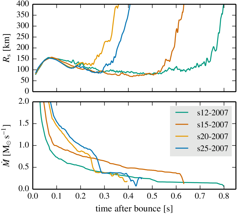
Figure 2.— Time evolution of average shock radius (upper panel) and mass-accretion rate (lower panel) for the simulations of Model Set I. Both quantities are averaged over all angular directions; the mass-accretion rate is evaluated at a radius of 400 km. The curves are smoothed by running averages of 5 ms.

The trajectories of the average shock radii are depicted in Fig. 2 (upper panel). All four models explode, but the post-bounce evolution differs. In the case of the two more massive progenitors of 20 M_⊙ and 25 M_⊙, the shock retreats until it encounters the Si/Si-O composition shell interface. This point in time is connected to a steep decrease of the mass-accretion rate (evaluated at a radius of 400 km, see lower panel of Fig. 2) given by

$$\dot{M}(r)=4\pi r^{2}\rho(r)|v(r)|.$$ (2)

Shortly afterwards, the shock starts to expand and the runaway conditions for an explosion are reached. This is different in the case of the two progenitors with lower masses of 12 M_⊙ and 15 M_⊙. Due to a much weaker density contrast at the Si/Si-O interface, the mass-accretion rate does not show a steep decline. It decreases more gradually and the two models explode at relatively late times. The difference in the explosion behavior between the two more massive and the two less massive progenitor models can be attributed to the competition of mass-accretion rate and neutrino energy deposition in the context of the delayed neutrino-driven explosion mechanism. The revival of the stalled shock front requires the neutrino heating to be strong enough to overcome the ram pressure of the infalling material (e.g. Burrows & Goshy, 1993; Janka & Müller, 1996; Janka, 2001; Murphy & Burrows, 2008; Fernández, 2012), and the threshold conditions for a successful explosion can be defined by a critical neutrino luminosity that depends on the mass-accretion rate of the shock (Burrows & Goshy, 1993). We will further elaborate on this aspect in Sect. 4, where we will discuss and demonstrate the influence of multidimensional fluid flows in the post-shock layer on the critical luminosity condition in a more general form introduced by Müller & Janka (2015).

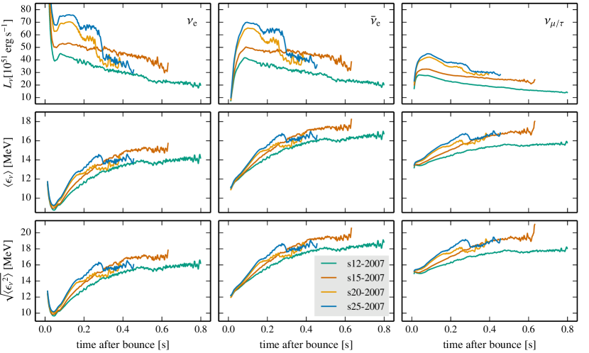
Figure 3.— Time evolution of neutrino luminosities (first row), neutrino mean energies (second row), and neutrino rms energies (third row) for the simulations of Model Set I (lab-frame quantities, evaluated at 400 km and given for an observer at infinity). From left to right, the angular averages are shown for $\nu_{\mathrm{e}}$, $\bar{\nu}_{\mathrm{e}}$, and $\nu_{\mu/\tau}$. The curves are smoothed by running averages of 5 ms.

In Fig. 3, the angle-averaged luminosities as well as the angle-averaged mean and rms energies of the different neutrino species are shown. These quantities are evaluated at 400 km and given for an observer in the lab frame at infinity. $\langle\epsilon_{\nu}\rangle$ and $\langle\epsilon_{\nu}^{2}\rangle$ are defined as the first and second moments of the dimensionless neutrino phase space distribution function $f(\epsilon,\mu)$,

$$\langle\epsilon_{\nu}^{n}\rangle=\frac{\int_{0}^{\infty}\mathrm{d}\epsilon_{\nu}\,\epsilon_{\nu}^{n}\,\epsilon_{\nu}^{2}\,\int_{-1}^{1}\mathrm{d}\mu\,f(\epsilon_{\nu},\mu)}{\int_{0}^{\infty}\mathrm{d}\epsilon_{\nu}\,\epsilon_{\nu}^{2}\,\int_{-1}^{1}\mathrm{d}\mu\,f(\epsilon_{\nu},\mu)},$$ (3)

where $\mu$ is the cosine of the angle between the neutrino momentum and the radial direction and $\epsilon_{\nu}$ the neutrino energy. Note that in the multidimensional case the additional directional averaging involves the integration of the numerator and denominator terms over all angular directions/bins of the computational grid.

Due to a higher mass-accretion rate and therefore a faster growth of the mass of the proto-neutron star, the two more massive models show higher neutrino luminosities and a faster growth of the radiated mean neutrino energies at early times of the post-bounce evolution. For this reason, neutrinos deposit more energy in the gain layer and provide stronger heating in the region behind the stalled shock. The arrival of the Si/Si-O composition shell interface at the shock is reflected by a drop of the neutrino luminosities and mean energies, which is further enhanced by the onset of shock expansion (see Fig. 3). At this time, the ram pressure of the infalling material is significantly reduced, but a lot of energy is still stored in the gain layer behind the shock due to the heating by the previously high accretion luminosities. This combination of high neutrino luminosities and mean energies but reduced ram pressure is very supportive for the revival of the shock (for a detailed discussion, see Ertl et al., 2016). In the two less massive progenitors, the Si/Si-O interface is relatively weak, and during the first 300 ms after bounce the neutrino luminosities and mean energies are lower. Therefore, it takes a longer time until the mass-accretion rate has decreased to such a low value that the ram pressure can be overcome by the neutrino heating.

The need for a favorable interplay between neutrino luminosity and mass-accretion rate with respect to the onset of a successful explosion is further supported by the results of our additional simulations of 14 pre-supernova models (Model Set II, see Sect. 3.2) and has been explored in a large set of 1D models by Ertl et al. (2016). In the following subsections, we will focus on the four simulations of Model Set I and investigate in detail the conditions that lead to the initiation of the explosion.

3.1.2 Conditions in the Gain Layer

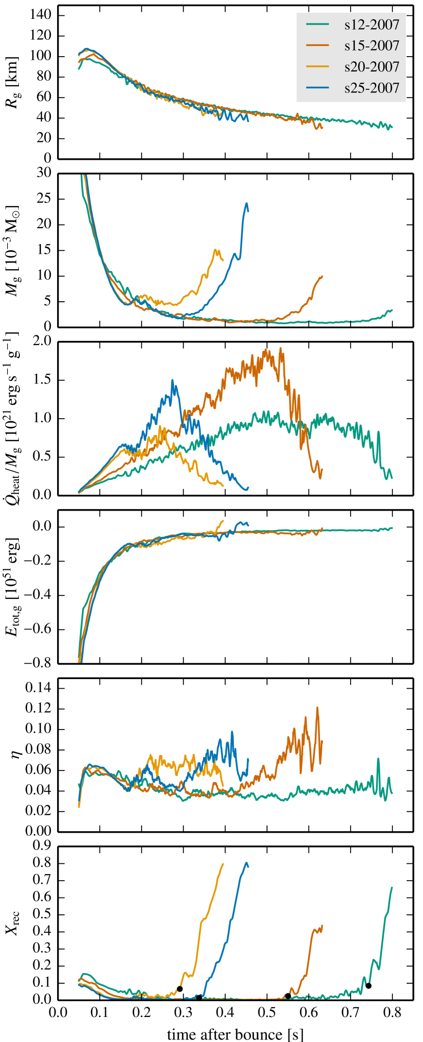
Figure 4.— Time evolution of gain radius, mass, neutrino heating rate per unit mass, total energy, neutrino heating efficiency, and the mass fraction of matter recombined to $\alpha$-particles and heavier nuclei in the gain layer (from top to bottom) for the four simulations of Model Set I. The black dots in the bottom panel mark the fraction of recombined matter at the time when the ratio $\tau_{\mathrm{adv}}/\tau_{\mathrm{heat}}$ reaches unity. Quantities that are not well defined shortly after bounce are only shown for $t\geq 0.05\,\mathrm{s}$. The curves are smoothed by running averages of 5 ms.

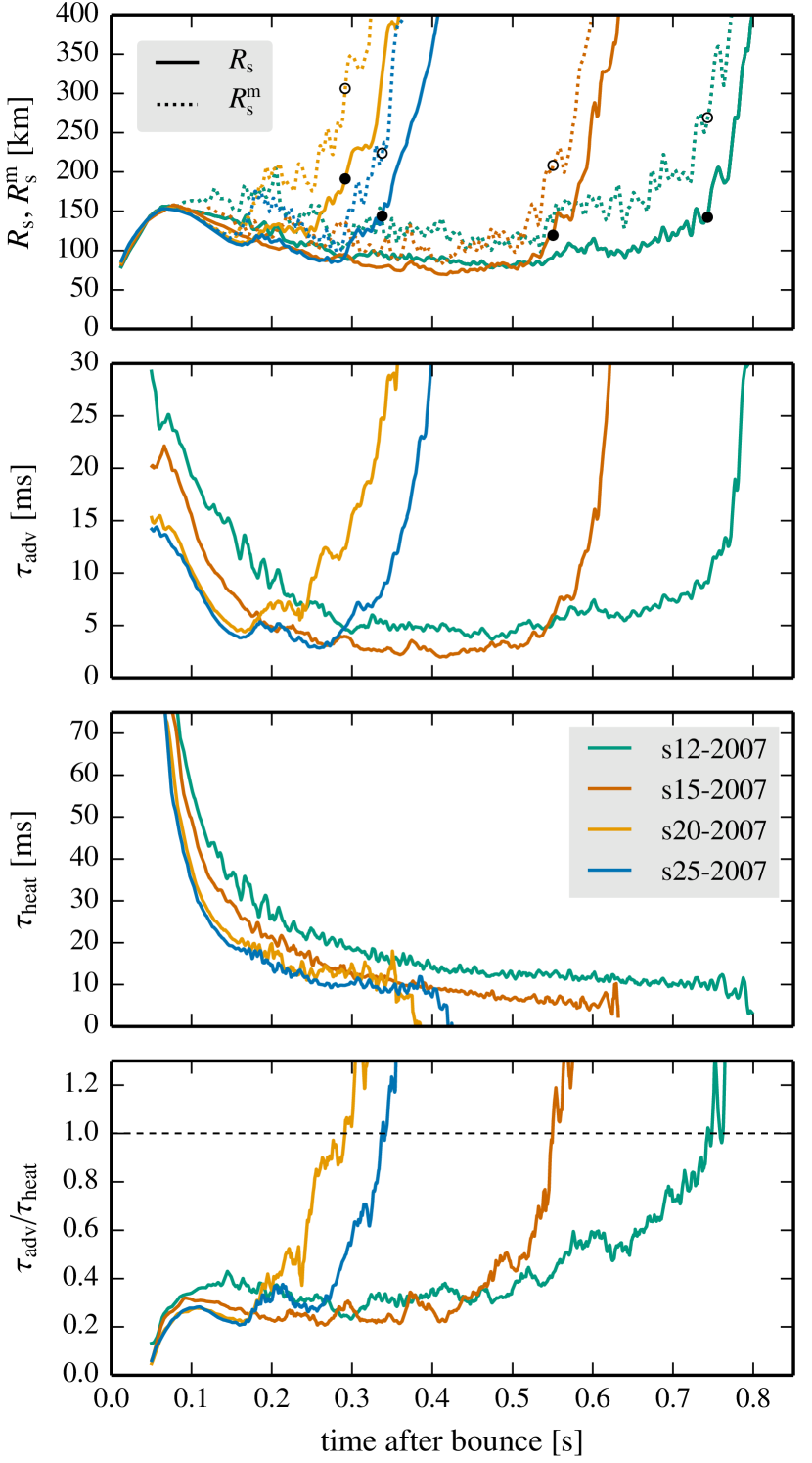
Figure 5.— Time evolution of average and maximum shock radius, advection and heating time scale as well as the ratio of the two time scales for the four simulations of Model Set I. The definitions of these quantities are given in the text. The black dots (open circles) in the top panel mark the value of the averaged (maximum) shock radius at the time when the ratio $\tau_{\mathrm{adv}}/\tau_{\mathrm{heat}}$ reaches unity. Quantities that are not well defined shortly after bounce are only shown for $t\geq 0.05\,\mathrm{s}$. The curves are smoothed by running averages of 5 ms.

The residence time of matter in the gain layer determines the exposure of this material to neutrino heating. If the advection time scale ($\tau_{\mathrm{adv}}$), defined as the time the accreted gas stays in the gain layer, is longer than the heating time scale ($\tau_{\mathrm{heat}}$), which is given by the time neutrino heating needs to deposit an energy equivalent to the binding energy of the gas, the conditions in the gain layer become advantageous for an explosion. For shock expansion to finally create a runaway situation, a sufficiently long period of $\tau_{\mathrm{adv}}/\tau_{\mathrm{heat}}\gtrsim 1$ is necessary (e.g. Janka et al., 2001; Thompson et al., 2005; Buras et al., 2006a; Fernández, 2012). In order to account for the influence of non-radial instabilities on the hydrodynamical flow in our 2D simulations, we follow Janka (2012) and Müller et al. (2012b) and use the dwell time of matter in the gain region as a measure for the average advection time scale, assuming quasi steady-state conditions (cf. Buras et al., 2006a; Marek & Janka, 2009):

$$\tau_{\mathrm{adv}}\coloneqq\tau_{\mathrm{dwell}}\approx\frac{M_{\mathrm{g}}}{\dot{M}}.$$ (4)

Here, $\dot{M}$ is the mass-accretion rate through the shock, and $M_{\mathrm{g}}$ is defined by the mass enclosed in the gain layer between the direction-dependent (i.e., dependent on the latitudinal angle) gain radius $R_{\mathrm{g}}(\theta)$ and shock radius $R_{\mathrm{s}}(\theta)$:

$$M_{\mathrm{g}}=\int\limits_{R_{\mathrm{g}}(\theta)<r<R_{\mathrm{s}}(\theta)}\rho\,\mathrm{d}V.$$ (5)

Our definition of the dwell time (Eq. 4) is only a rough approximation of the advection time scale of matter falling inward through the gain layer, because this expression also includes material rising with positive velocities. For exactly this reason, however, Eq. (4) is a good measure of the residence time of matter in the neutrino-heated region, because the time period of gas being exposed to neutrino heating is increased by non-radial as well as outward mass motions, which are responsible for a growth of the mass in the gain layer. Naturally, after the onset of the explosion, expanding matter begins to dominate in the gain layer, for which reason Eq. (4) does not yield a good representation of the “advection time scale” any longer.

The heating time scale is defined by the ratio of the total energy of the material in the gain layer and the volume-integrated neutrino heating rate in this region,

$$\tau_{\mathrm{heat}}=\frac{\left|E_{\mathrm{tot,g}}\right|}{\dot{Q}_{\mathrm{heat}}}.$$ (6)

The total energy in the gain layer is given by the integral over the sum of specific kinetic energy, $v^{2}/2$, specific internal energy, $\epsilon$, and specific gravitational binding energy,

$$E_{\mathrm{tot,g}}=\int\limits_{R_{\mathrm{g}}(\theta)<r<R_{\mathrm{s}}(\theta)}\rho\left[\left(\frac{v^{2}}{2}+\epsilon\right)+\Phi\right]\mathrm{d}V,$$ (7)

with $\Phi$ being the gravitational potential. The neutrino heating rate is the integral of the neutrino energy deposition rate per volume $q_{\mathrm{e}}$ over the gain layer

$$\dot{Q}_{\mathrm{heat}}=\int\limits_{R_{\mathrm{g}}(\theta)<r<R_{\mathrm{s}}(\theta)}q_{\mathrm{e}}\,\mathrm{d}V.$$ (8)

In Figs. 4 and 5, different diagnostic quantities evaluated for the gain region are presented during the post-bounce evolution. While the heating time scale continuously decreases with time, the advection time scale shows a rapid increase at the time of the arrival of the Si/Si-O interface in the case of the two more massive models (see Fig. 5). This increase is caused by the sudden decline of the mass-accretion rate (cf. Fig. 2, lower panel). The longer residence time of matter in the gain region thus enables more efficient neutrino heating (Fig. 4, fifth panel from top) providing the power to drive the shock outwards.

The advection time scale of the two less massive models shows a continuous decrease connected to the diminishing amount of mass contained in the gain layer (see Fig. 4, second panel from top) until it stabilizes on a level around 5 ms. Nevertheless, these two models still explode at relatively late times after bounce. This can be attributed to the increasing heating efficiency (see Fig. 4, lower panel) defined by the ratio of the total energy deposition rate to the sum of the radiated electron neutrino and electron antineutrino luminosities (which dominate the heating rate through $\nu_{\mathrm{e}}$ and $\bar{\nu}_{\mathrm{e}}$ absorption on free nucleons):

$$\eta=\frac{\dot{Q}_{\mathrm{heat}}}{L_{\nu_{\mathrm{e}}}+L_{\bar{\nu}_{\mathrm{e}}}},$$ (9)

where we measure the luminosities at a radius of 400 km. Following Janka (2001, 2012), the neutrino energy deposition in the gain layer scales with $L_{\nu_{\mathrm{e}}}$, $L_{\bar{\nu}_{\mathrm{e}}}$, $\langle E_{\nu_{\mathrm{e}}}^{2}\rangle$, $\langle E_{\bar{\nu}_{\mathrm{e}}}^{2}\rangle$, and $M_{\mathrm{g}}$ as

$$\dot{Q}_{\mathrm{heat}}\propto\frac{L_{\nu_{\mathrm{e}}}\langle E_{\nu_{\mathrm{e}}}^{2}\rangle+L_{\bar{\nu}_{\mathrm{e}}}\langle E_{\bar{\nu}_{\mathrm{e}}}^{2}\rangle}{R^{2}_{\mathrm{g}}}M_{\mathrm{g}}.$$ (10)

Note that $\langle E_{\nu_{\mathrm{e}}}^{2}\rangle\coloneqq\langle\epsilon_{\nu_{\mathrm{e}}}^{3}\rangle/\langle\epsilon_{\nu_{\mathrm{e}}}\rangle$ and $\langle E_{\bar{\nu}_{\mathrm{e}}}^{2}\rangle\coloneqq\langle\epsilon_{\bar{\nu}_{\mathrm{e}}}^{3}\rangle/\langle\epsilon_{\bar{\nu}_{\mathrm{e}}}\rangle$ are defined from the energy distribution of neutrinos in energy space, not from the number distribution as $\langle\epsilon_{\nu_{\mathrm{e}}}^{2}\rangle$ and $\langle\epsilon_{\bar{\nu}_{\mathrm{e}}}^{2}\rangle$. Since the mass in the gain layer (see Fig. 4, second panel from top) is growing at later times and the neutrino rms energies (see Fig. 3, third row) are continuously increasing, too, the slow decline of the accretion luminosity (see Fig. 3, first row) can be overcompensated and the heating efficiency rises noticeably already before the onset of the explosion (cf. Marek & Janka, 2009; Müller et al., 2012b). This effect can be observed in the two less massive models: At late times, $\nu_{\mathrm{e}}$ and $\bar{\nu}_{\mathrm{e}}$ deposit a larger fraction of their energy in the gain layer, the post-shock flow is heated more efficiently and finally an explosion is triggered.

Around the onset of the explosion, the advection time scale rises steeply in all four models. Higher pressure and stronger “turbulent” flows in the gain layer lead to an expansion of gas outward from deeper layers of the gain region. The expansion of the shock creates a positive feedback loop by further increasing the advection time scale. Once the critical condition of $\tau_{\mathrm{adv}}/\tau_{\mathrm{heat}}\gtrsim 1$ is reached, a runaway situation with continuous shock expansion is created (e.g. Buras et al., 2006b; Murphy & Burrows, 2008; Fernández, 2012). The evolution of the total energy in the gain layer can be inferred from Fig. 4 (fourth panel from top). When the time-scale ratio $\tau_{\mathrm{adv}}/\tau_{\mathrm{heat}}$ reaches unity, the total energy is still slightly negative (compare Figs. 4 and 5; cf. also Janka, 2001; Fernández, 2012). At the beginning of the shock expansion, just a small fraction of the material in the gain layer is rising while most parts of the matter behind the shock are still nearly at rest (see also Sect. 3.1.3). Only when the whole gain layer starts to expand, does the total energy tend towards positive values indicating that the post-shock material gets unbound in the gravitational field created by the enclosed mass. In Fig. 6, the average entropy in the gain layer, defined by

$$\langle s_{\mathrm{g}}\rangle=\frac{1}{M_{\mathrm{g}}}\int\limits_{R_{\mathrm{g}}(\theta)<r<R_{\mathrm{s}}(\theta)}s\,\rho\,\mathrm{d}V,$$ (11)

as well as the maximum entropy and the mass in the gain layer with entropies above the average value are given. In all four models, the entropy increases towards explosion. On the way to explosion also the mass in the gain layer with entropies above the average value is growing, which is compatible with previous findings that the masses and volumes with entropies above certain threshold values grow (Nordhaus et al., 2010; Hanke et al., 2012; Fernández et al., 2014). Although models exploding at later times after bounce show a tendency towards higher entropies, no generic value that signals the successful runaway can be found. Once the explosion has started, a great amount of lower-entropy gas from below the gain radius enters the gain layer and leads to a drop of the average entropy by $2-4\,k_{\mathrm{B}}$ per nucleon.

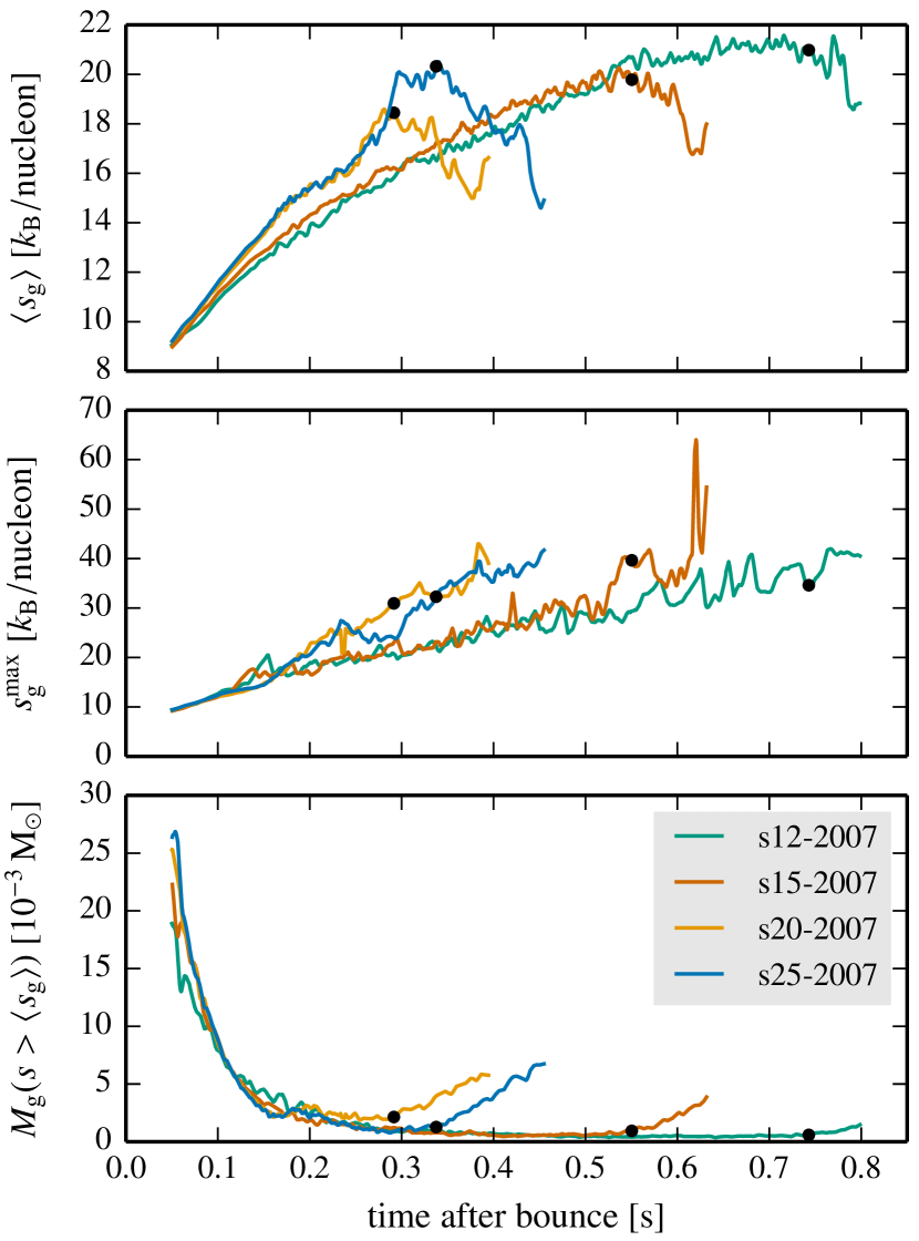
Figure 6.— Time evolution of average and maximum entropy in the gain layer as well as the mass in the gain layer with entropies above the average value (from top to bottom). The black dots mark the point in time when the ratio $\tau_{\mathrm{adv}}/\tau_{\mathrm{heat}}$ reaches unity. The quantities are shown for $t\geq 0.05\,\mathrm{s}$ and the curves are smoothed by running averages of 5 ms.

Overall, the time-scale criterion seems to be a viable concept for interpreting the explosion behavior of all four models. We will provide further evidence for that in Sect. 4. The concept is post-dictive in the sense that it is based on an analysis of the model conditions (in contrast to a two-parameter criterion found by Ertl et al. (2016), which is based on the properties of the pre-collapse star). There is ongoing controversy in the literature whether better explosion indicators exist that describe the approach to runaway shock expansion in a physically more founded way (e.g. Pejcha & Thompson, 2012; Murphy & Dolence, 2015; Gabay et al., 2015). We do not want to take a position in the debate here because we focus on multidimensional results while the cited literature discusses the behavior of the shock-stagnation problem in 1D, where special pathologies like large-scale radial shock pulsations can occur, which do not have a direct counterpart in 2D and 3D. Janka (2012) and Müller & Janka (2015) have shown that the critical condition of the time-scale ratio can formally be connected to the critical luminosity condition $L_{\mathrm{crit}}(\dot{M})$ introduced by Burrows & Goshy (1993); see also, e.g., Yamasaki & Yamada (2005), Murphy & Burrows (2008), Nordhaus et al. (2010), Hanke et al. (2012), and Fernández (2012), which can be generalized to include the effects of non-radial fluid flows in terms of a contribution by turbulent pressure (cf. Müller & Janka, 2015). In Sect. 4, we follow the approach of Müller & Janka (2015) and demonstrate that a generalized critical condition can be formulated that applies to the whole set of 18 models as a general criterion for the onset of the explosion.

In multidimensional simulations, the development towards a runaway situation is closely connected to the evolution of hydrodynamic instabilities. The growth conditions of these instabilities are the topic of the next subsection, where their properties are further discussed in dependence on the different progenitor models.

3.1.3 Growth of Instabilities

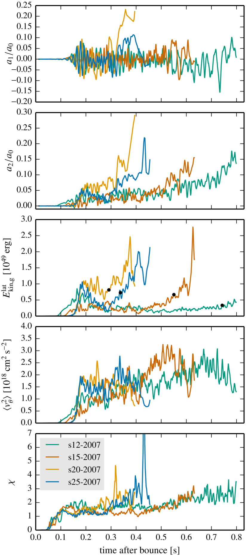
Figure 7.— Time evolution of the coefficients $a_{1}$ (dipole mode, first panel) and $a_{2}$ (quadrupole mode, second panel) for an expansion of the shock surface into Legendre polynomials. The coefficients are normalized to the amplitude of the $l=0$ mode (i.e. the average shock radius). Furthermore, the kinetic energy of lateral mass motions (third panel) and the velocity dispersion in the gain layer (fourth panel) are given. The black dots in the third panel mark the kinetic energy level at the time when the ratio $\tau_{\mathrm{adv}}/\tau_{\mathrm{heat}}$ reaches unity. In the bottom panel, the growth parameter $\chi$ is depicted for the four simulations of Model Set I. All curves are smoothed by running averages of 5 ms.

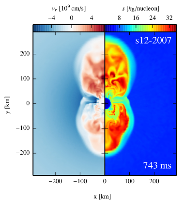
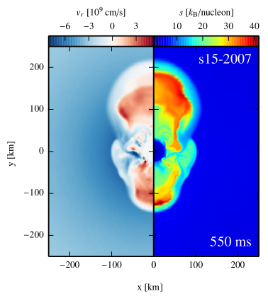
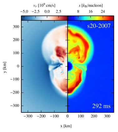
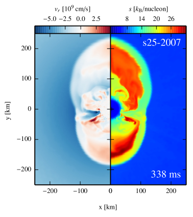
Figure 8.— Snapshots of radial velocity (left halfs of the panels) and entropy per baryon (right halfs of the panels) for the four simulations of Model Set I at the time of explosion (defined by the time when the ratio $\tau_{\mathrm{adv}}/\tau_{\mathrm{heat}}$ reaches unity).

Non-radial mass motions are crucial for an increase of the dwell time of matter in the gain layer, enhanced neutrino heating, turbulent pressure, and the subsequent expansion of the shock radius (Murphy et al., 2013; Müller & Janka, 2015). Both convection and the standing accretion-shock instability (SASI, Blondin et al., 2003) can provide sufficient support to the neutrino-heating mechanism to finally revive the previously stalled shock front. Typically, the high mass-accretion rates of the investigated models (see Fig. 2, lower panel) and the decreasing neutron star radii (see Fig. 10, second panel) lead to very small shock radii stabilizing at $\sim 80\,\mathrm{km}$, well following the proportionality

$$R_{\mathrm{s}}\propto\frac{\left(L_{\nu}\langle E_{\nu_{\mathrm{e}}}^{2}\rangle\right)^{4/9}R_{\mathrm{NS}}^{16/9}}{\dot{M}^{2/3}M_{\mathrm{NS}}^{1/3}}$$ (12)

(Janka, 2012) as soon as quasi-steady state accretion conditions in the post-shock layer apply and as long as multidimensional effects do not play a crucial role (for a generalization to multi-dimensions, see Eq. (29) below and Müller & Janka, 2015). Due to the scaling relation (cf. Scheck et al., 2008)

$$\tau_{\mathrm{adv}}\propto R_{\mathrm{s}}^{3/2},$$ (13)

the advection time scale shrinks accordingly. The linear growth rate $\omega_{\mathrm{SASI}}$ of the advective-acoustic cycle amplifying the SASI growth is given by (Foglizzo et al., 2006)

$$\omega_{\mathrm{SASI}}=\frac{\mathrm{ln}|\mathcal{Q}|}{\tau_{\mathrm{cyc}}},$$ (14)

where $\mathcal{Q}$ is the efficiency and $\tau_{\mathrm{cyc}}$ is the duration of the cycle. As argued by Scheck et al. (2008) and Müller et al. (2012a), $\tau_{\mathrm{cyc}}$ is short for small shock radii and thus short advection time scales. Hence, our models with rather short advection time scales should provide favorable conditions for efficient SASI growth. In order to quantify this expected behavior by a detailed analysis, we decompose the angle-dependent shock surface $R_{\mathrm{s}}(\theta)$ into Legendre polynomials $P_{l}(\cos\theta)$. The expansion coefficients are defined by (Burrows, 2012; Ott et al., 2013)

$$a_{l}=\frac{1}{2}\int\limits_{0}^{\pi}R_{\mathrm{s}}(\theta)\,P_{l}(\cos\theta)\,\mathrm{d}(\cos\theta).$$ (15)

For the four models of Model Set I, the time evolution of the coefficient $a_{1}$ (dipole mode) is shown in Fig. 7 (upper panel). At $\sim 120\,\mathrm{ms}$ after bounce (average shock radii between 120 km and 150 km, see Fig.2, first panel), shock sloshing motions begin to grow in the well-known oscillatory way. At this time, the lateral kinetic energy in the gain region increases (see Fig. 7, third panel from top) and the post-shock flow becomes aspherical. All models exhibit strong quasi-periodic shock oscillations with oscillation periods of 15 ms to 20 ms. At $\sim 220\,\mathrm{ms}$ after bounce, the Si/Si-O composition shell interface reaches the shock in the case of the two more massive models, and the advection time scale and hence the SASI oscillation period increase (Foglizzo et al., 2007; Scheck et al., 2008; Guilet & Foglizzo, 2012). During the shock expansion phase, the two models still show large shock oscillations, but these oscillations are less regular than before. In the two less massive models, shock oscillations with short periods can be maintained up to several hundred milliseconds after bounce. Only after the shock expansion sets in, can larger SASI amplitudes with non-periodic behavior and large shock excursions with unipolar or bipolar asymmetry be observed.

The time evolution of the quadrupole mode represented by the coefficient $a_{2}$ is depicted in Fig. 7 (second panel from top). Shortly before shock expansion sets in, all four models develop a growing prolate quadrupolar deformation of the shock surface. In the two more massive models that develop explosions at earlier times, the $a_{2}$ coefficient almost continuously increases directly from the onset of SASI activity at $\sim 120\,\mathrm{ms}$. In the case of the less massive models exploding at later times, the increase of the quadrupole mode starts at $\sim 450\,\mathrm{ms}$. The development of a strong quadrupole mode in all four models is a serious hint that the artificial symmetry axis introduced in 2D simulations may play a supportive role for the runaway expansion of the shock (e.g. Takiwaki et al., 2012; Hanke et al., 2012; Couch, 2013). The quadrupole mode periodically pushes the post-shock layer further and further out towards the polar direction along the symmetry axis, while inflow occurs along funnels near the equator. The big polar, buoyant bubbles are fed by material from equatorial downflows, which channel accreted matter to the gain radius, where it can be efficiently heated by neutrinos.

The large-amplitude bipolar oscillations with increasing amplitudes push the shock front step by step outwards to larger radii. Due to the effective increase of the dwell time of matter that is channelled into the polar lobes, more accreted material can be heated by the neutrinos for longer times (see bottom panel of Fig. 4 for the growing neutrino heating efficiency). The continuously ongoing SASI oscillations successively drive the shock front outwards, which in turn further increases (cf. Eq. 4) the advection time scale of matter in the gain layer. This positive feedback loop finally induces a successful explosion (Marek & Janka, 2009; Müller et al., 2012b).

Additionally, the supportive role of the SASI for shock revival is mirrored in supersonic lateral velocities (sound speed $c_{\mathrm{s}}\sim 10^{9}\,\mathrm{cm\,s}^{-1}$) in the post-shock flow caused by repeated phases of large-amplitude shock expansion and contraction. The kinetic energy of these non-radial mass motions shows quasi-periodic variations with spiky maxima (see Fig. 7, third panel from top). As pointed out by Hanke et al. (2012), this is typical of the presence of low-order SASI modes. Similar to the results of their parametric study for models at the explosion threshold, the successful explosions presented here are triggered and accompanied by large-scale mass flows, which are indicated by growing fluctuations of the angular kinetic energy that are characteristic for strong SASI activity.

While the lateral kinetic energy also depends on the mass contained in the gain region, the velocity dispersion $\langle v_{\theta}^{2}\rangle$ provides a direct measure for the typical velocities of convective and SASI motions and for the turbulent pressure associated with them (Müller & Janka, 2015). Consequently, the continuous growth of this quantity for all models indicates an increase of convective and SASI activity with time. This is especially supportive for the development of an explosion at several hundred milliseconds after bounce in the case of the two less massive models. Following Müller & Janka (2015), the lateral kinetic energy satisfies the relation

$$\frac{E_{\mathrm{kin,g}}^{\mathrm{lat}}}{M_{\mathrm{g}}}\propto\left[\left(\langle R_{\mathrm{s}}\rangle-\langle R_{\mathrm{g}}\rangle\right)\frac{\dot{Q}_{\mathrm{heat}}}{M_{\mathrm{g}}}\right]^{2/3}.$$ (16)

Since the neutrino heating rate per unit of mass, $\dot{Q}_{\mathrm{heat}}/M_{\mathrm{g}}$, scales with $L_{\nu_{\mathrm{e}}}\langle E_{\nu_{\mathrm{e}}}^{2}\rangle+L_{\bar{\nu}_{\mathrm{e}}}\langle E_{\bar{\nu}_{\mathrm{e}}}^{2}\rangle$ (cf. Eq. 10 and see Fig. 4, third panel from top), the continuous increase of the mean neutrino energies is also responsible for the growth of the velocity dispersion and fosters the large-scale aspherical mass motions which finally induce the onset of explosion.

While the conditions of the hydrodynamic post-shock flow are favorable for the efficient development of the SASI in our simulations, convection is generally suppressed. Similar to the results of Scheck et al. (2008) and Marek & Janka (2009), the neutrino energy deposition in the gain layer of our models is too weak to generate a steep negative entropy gradient. The latter is a prerequisite for the development of convection. Furthermore, the applied EoS of Lattimer & Swesty (1991) with a nuclear incompressibility of 220 MeV generates rather compact neutron stars (Steiner et al., 2010; Hebeler et al., 2010). Thus, the forming neutron stars contract rapidly from a maximum radius of $\sim 75\,\mathrm{km}$ to $\sim 40\,\mathrm{km}$ after 200 ms post bounce and $\sim 25\,\mathrm{km}$ after $\sim 800\,\mathrm{ms}$ post bounce. Since the shock radius directly scales with the neutron star radius (measured by the radial location of $\rho=10^{11}\,\mathrm{g\,cm}^{-3}$; see Eq. 12), the contraction of the neutron star also enforces the retraction of the shock radius. That is why the matter in the post-shock region is rapidly advected towards the gain radius and the growth of convective motions is suppressed (cf. Foglizzo et al., 2006).

In order to quantify the importance of convection, we determine the growth parameter $\chi$ introduced by Foglizzo et al. (2006) for our four explosion models (see Fig. 7, lower panel). This parameter can be considered as a measure of the ratio of the advection time scale of the flow through the gain layer and the growth time scale of convection. It is defined in terms of the Brunt-Väisälä frequency $\langle\omega_{\mathrm{BV}}\rangle$ (calculated from angle-averaged quantities, for a discussion see Fernández et al., 2014) and the spherically averaged advection velocity $\langle v_{r}\rangle$ by

$$\chi=\int\limits_{\langle R_{\mathrm{g}}\rangle}^{\langle R_{\mathrm{s}}\rangle}\frac{\mathrm{Im}\,\langle\omega_{\mathrm{BV}}\rangle}{|\langle v_{r}\rangle|}\mathrm{d}r,$$ (17)

where the integration runs from the averaged gain radius to the averaged shock radius. Only regions with $\omega_{\mathrm{BV}}^{2}<0$ (indicating local instability) contribute to the integral. Since perturbations are advected out of the gain layer with the accretion flow in a finite time, a sufficient amplification of initial perturbations within this time interval is needed for the successful development of convective motions. According to the analysis of Foglizzo et al. (2006) in the linear regime of small initial perturbations, a threshold condition of $\chi\gtrsim 3$ is necessary for convective instability in the gain region. This condition is compatible with several numerical studies in 2D (e.g. Buras et al., 2006a; Scheck et al., 2008; Fernández & Thompson, 2009; Fernández et al., 2014).

While SASI activity starts at around $\sim 100\,\mathrm{ms}$ after bounce when aspherical mass motions begin to develop (see Fig. 7, two upper panels), the growth parameter for convective instability still remains subcritical (see Fig. 7, lower panel). Due to the low neutrino heating rates and the small shock radii and correspondingly short advection time scales at these times, convection is damped in all four models. This absence of convection may also be supportive for the early development of the SASI (cf. Müller et al., 2012a). In the case of the two more massive models, the threshold condition of $\chi>3$ is reached after the Si/Si-O composition shell interface has arrived at the shock. Because of the abruptly reduced mass accretion rate, the shock expands to larger radii and the advection time scale rises. This leads to increased values of $\chi$.

The two less massive models retain a subcritical value of $\chi$ for a long time. After $\sim 500\,\mathrm{ms}$, the conditions for convection become more and more favorable. Convective activity is fully established when the time-scale ratio $\tau_{\mathrm{adv}}/\tau_{\mathrm{heat}}$ exceeds unity and shock expansion sets in. The reason for the gradual development of convection in these two models is two-fold. On the one hand, the large-amplitude SASI sloshing motions of the stalled shock front are associated with fast lateral flows in the post-shock region (see Fig. 7, third and fourth panel from above) and induce the formation of layers with very steep unstable entropy gradients (see also Scheck et al., 2008; Marek & Janka, 2009). This supports the emergence of secondary convective activity (Buras et al., 2006a; Scheck et al., 2008). On the other hand, the increasing values of the $\chi$ parameter directly mirror the enhanced neutrino energy deposition per unit of mass (see Fig. 4, third panel from top) at late times.

While our simulations show a similar behavior as the “SASI-dominated” model s27.0 presented by Müller et al. (2012a), a clear disentanglement of SASI and convective effects with respect to the post-shock dynamics emerging around shock revival is difficult. In the case of strongly aspherical flows due to the SASI, with perturbations far away from the linear regime, the criterion $\chi>3$ may no longer be a reliable measure for the development of convective instability. To illustrate the hydrodynamic properties of the post-shock flow around shock revival, color-coded snapshots of entropy and radial velocity are presented in Fig. 8 for all models at the time when the time-scale ratio $\tau_{\mathrm{adv}}/\tau_{\mathrm{heat}}$ reaches unity. All models show a prolate deformation of the shock surface caused by large-amplitude bipolar SASI oscillations. In addition to small buoyant bubbles growing in the wake of the SASI sloshing motions, large-scale high-entropy bubbles triggered by the SASI shock expansion phases are visible. Due to the assumption of axisymmetry, large plumes preferentially grow along the direction of the artificial symmetry axis (see also Takiwaki et al., 2012; Hanke et al., 2012; Couch, 2013).

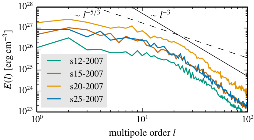
Figure 9.— Turbulent energy spectra $E(l)$ as functions of the multipole order $l$. The spectra are based on a decomposition of the azimuthal velocity $v_{\theta}$ into spherical harmonics 25 ms before the time-scale ratio $\tau_{\mathrm{adv}}/\tau_{\mathrm{heat}}$ exceeds unity, averaged over a time interval of 5 ms and a radius interval from 50 km to 80 km. The thin dashed and solid black lines indicate reference spectral slopes of $-5/3$ and $-3$.

According to Fernández et al. (2014), SASI-dominated explosion models are characterized by the interplay of shock sloshing motions and the formation of large-scale, high-entropy structures. The authors conclude that a SASI-driven explosion develops if these bubbles are able to survive during several SASI oscillation periods. The dominance of large-scale bubbles seeded by SASI sloshing motions compared to small-scale bubbles driven by convection as indicated by the snapshots in Fig. 8 clearly suggests that the post-shock flow dynamics in our simulations are governed by the SASI while convective instabilities play a more secondary role. This interpretation is further supported by an analysis of the energy spectrum $E(l)$ which considers the decomposition of the azimuthal velocity $v_{\theta}$ at a given radius (weighted by the square root of the density) into spherical harmonics $P_{l}(\cos\theta)$ as the 2D analogon of the definition provided by Hanke et al. (2012):

$$E(l)=\frac{1}{2}\left|\sqrt{\left(2l+1\right)\pi}\int\limits_{0}^{\pi}P_{l}\left(\cos\theta\right)\sqrt{\rho}\,v_{\theta}\left(r,\theta\right)\mathrm{d}(\cos\theta)\right|^{2}.$$ (18)

The results of this analysis are shown in Fig. 9. In order to obtain smoother spectra, $E(l)$ is averaged over 30 km in radius and over 5 ms in time. Similar to the SASI-dominated models discussed by Fernández et al. (2014), the angular spectrum of all four models shows a peak at $l=2$. The strong presence of convection is visible from the enhanced power in the $l=5-10$ domain fully compatible with the spectral features observed in the convection dominated models by Fernández et al. (2014). This confirms the fact that the $\chi$ parameter tends towards the critical value of 3 or even begins to exceed this value when the time-scale ratio approaches unity. The slope of $\sim-3$ at large $l$ is indicative for a direct vorticity cascade being characteristic of the spectral properties of turbulence in axisymmetry (Kraichnan, 1967).

3.1.4 Diagnostic Explosion Energies and Neutron Star Properties

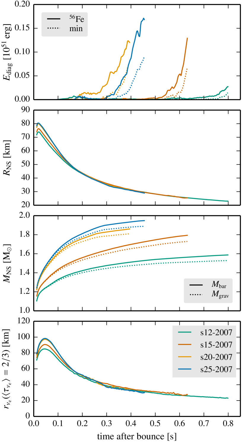
Figure 10.— Time evolution of diagnostic energy (lower limits indicated by dotted lines, upper limits by solid lines, see text), neutron star radius and mass (the baryonic mass is denoted by solid lines, the gravitational mass by dotted lines), and the radius of the spectrally averaged $\nu_{\mathrm{e}}$ sphere at an optical depth of $\langle\tau_{\nu_{\mathrm{e}}}\rangle=2/3$ (from top to bottom). Neutron star radius and mass are defined by the density surface at $10^{11}\,\mathrm{g}\,\mathrm{cm}^{-3}$. All quantities are angle-averaged and the curves are smoothed by running averages of 5 ms.

The diagnostic energies depicted in Fig. 10 (dotted lines in upper panel) are calculated by integrating over the gain layer for regions where the total specific energy defined as $e_{\mathrm{tot}}=v^{2}/2+\epsilon+\Phi$ is positive (see also previous studies by Buras et al., 2006b; Marek & Janka, 2009; Suwa et al., 2010; Müller et al., 2012b; Bruenn et al., 2013):

$$E_{\mathrm{diag}}=\int\limits_{R_{\mathrm{g}}(\theta)<r<R_{\mathrm{s}}(\theta)}e_{\mathrm{tot,>0}}\,\rho\,\mathrm{d}V.$$ (19)

In addition to this lower limit, we also show diagnostic explosion energies obtained by the assumption that all nucleons finally recombine to iron-group nuclei, which accounts for the maximum release of nuclear binding energy and can be considered as upper limit (see Fig. 10, solid lines in upper panel). Typically, first fluid elements behind the shock become formally unbound ($e_{\mathrm{tot}}>0$) at the onset of the explosion when the time-scale ratio exceeds unity. After the shock has expanded beyond $\sim 200\,\mathrm{km}$, the temperature behind the shock decreases sufficiently to allow for the recombination of nucleons to $\alpha$-particles (see bottom panel of Fig. 4 for the fraction $X_{\mathrm{rec}}$ of recombined matter in the gain layer). Consequently, the explosion energy starts to rise with a steep gradient. At the time our simulations had to be stopped because of the extremely high computational demands of the neutrino transport, maximum diagnostic energies of up to $\sim 0.17\times 10^{51}\,\mathrm{erg}$ were reached and were still increasing steeply.

However, at this stage of the simulations a reliable determination of the final explosion energies is not possible. In order to follow the energy budget of unbound matter and the continuous recombination processes behind the expanding shock front, the simulations would have to be carried on further for several hundred milliseconds (cf. Scheck et al., 2006, 2008). This is presently beyond reach due to extremely small transport time steps. Because of ongoing accretion and mass ejection we expect that the explosion energies can rise considerably even after the onset of the explosion (cf. Marek & Janka, 2009; Müller et al., 2012b; Müller, 2015).

The time evolution of the baryonic and gravitational neutron star masses and radii defined by the density surface at $10^{11}\,\mathrm{g}\,\mathrm{cm}^{-3}$ as well as the radius of the spectrally averaged electron neutrino sphere at an (effective) optical depth of $\langle\tau_{\nu_{\mathrm{e}}}\rangle=2/3$ is shown in the three lower panels of Fig. 10. For computing the optical depth for neutrino equilibration we used the effective opacity

$$\kappa_{\mathrm{eff}}=\sqrt{\kappa_{\mathrm{tot}}\,\kappa_{\mathrm{abs}}},$$ (20)

where $\kappa_{\mathrm{abs}}$ is the opacity for neutrino absorption processes and $\kappa_{\mathrm{tot}}=\kappa_{\mathrm{abs}}+\kappa_{\mathrm{scatt}}$ is the total opacity for absorption and scattering. The preliminary value of the neutron star mass is determined by the amount of matter that can be accreted from the collapsing star and settles to densities above $10^{11}\,\mathrm{g\,cm}^{-3}$ until the end of our simulations. After the strong decrease of the mass-accretion rate caused by the arrival of the Si/Si-O interface in the two more massive models, the increase of the neutron star masses begins to flatten. The higher growth rate of the neutron star mass in model s15-2007 compared to model s12-2007 directly reflects the differences of the mass-accretion rates in these two simulations that persist until the explosions set in at late times (compare Fig. 2).

3.2. Model Set II

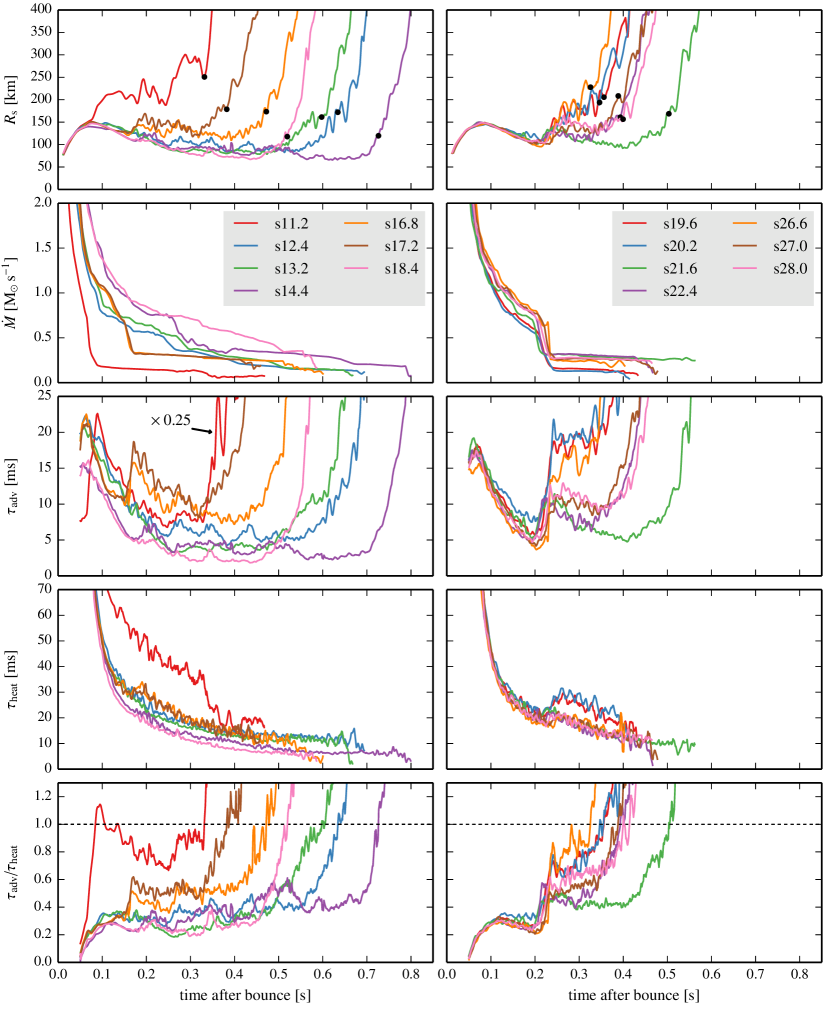
Figure 11.— Time evolution of different diagnostic quantities for Model Set II. For better clarity, the 14 models are subdivided into two parts: the models with lower ZAMS masses are displayed in the left column, the models with higher ZAMS masses in the right column. From top to bottom, the average shock radius, the mass-accretion rate, the advection time scale, the heating time scale, and the time-scale ratio are depicted. Quantities that are not well defined shortly after bounce are only shown for $t\geq 0.05\,\mathrm{s}$ post bounce. The black dots in the top panels mark the point in time when the ratio $\tau_{\mathrm{adv}}/\tau_{\mathrm{heat}}$ reaches unity (in the case of model s11.2, the transient spike of $\tau_{\mathrm{adv}}/\tau_{\mathrm{heat}}\gtrsim 1$ at early times was disregarded). Note that the advection time scale of model s11.2 (left column, third panel from top) is scaled with a factor of 0.25. All quantities are angle-averaged and the curves are smoothed by running averages of 5 ms.

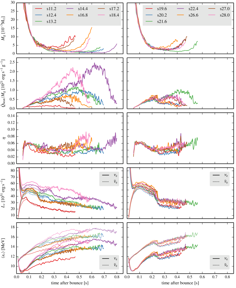
Figure 12.— Time evolution of different diagnostic quantities for Model Set II. For better clarity, the 14 models are subdivided into two parts: the models with lower ZAMS masses are displayed in the left column, the models with higher ZAMS masses in the right column. From top to bottom, the mass in the gain layer, the neutrino heating rate per unit mass, the neutrino heating efficiency, and the luminosities and mean energies of electron neutrinos (solid lines) and electron antineutrinos (dotted lines) are depicted. Quantities that are not well defined shortly after bounce are only shown for $t\geq 0.05\,\mathrm{s}$ post bounce. All quantities are angle-averaged and the curves are smoothed by running averages of 5 ms.

In the following, the main results of our simulations (Set II) concerning 14 pre-supernova models of Woosley et al. (2002) are presented in the light of the preceding discussion of Set I. An overview of the characteristic properties of these models is given in Figs. 11 and 12.

The differences in the position and density gradient of the Si/Si-O interface (see Fig. LABEL:denplot) are directly mirrored by the temporal evolution of the mean shock radii of the models with lower and higher ZAMS masses (see Fig. 11, first row). The most outstanding examples are models s19.6, s20.2, and s26.6 with a very pronounced jump of the density at the interface. After the arrival of this jump at the shock surface, the shock almost continuously expands outwards. The time evolution of these models is comparable to that of models s20-2007 and s25-2007 extensively discussed in Sect. 3.1. For model s21.6, the delay between the arrival of the interface and the beginning of the shock expansion is largest, because for this model the step-like decrease of the mass-accretion rate is less extreme than in the other representatives of the subset of more massive models (see Fig. 11, second row). The less massive stars that do not show a sharp discontinuity at the Si/Si-O interface (especially the 12.4 M_⊙, 13.2 M_⊙, 14.4 M_⊙, and 18.4 M_⊙ cases) explode only at relatively late times when the mass-accretion rates have decreased sufficiently, similar to the models s12-2007 and s15-2007 of Model Set I.

Model s11.2 which has already been intensively studied in previous works (Buras et al., 2006a; Marek & Janka, 2009; Müller et al., 2012b; Suwa et al., 2013) can be considered as special case. In this model, the Si/Si-O composition shell interface arrives already at $\sim 80\,\mathrm{ms}$ after bounce and at this time, the mass-accretion rate decreases to a much lower value ($\sim 0.2\,\mathrm{M}_{\odot}\,\mathrm{s}^{-1}$) than in the other less massive models. This is why the shock front can expand to large radii at early times. In spite of a transient overshoot of $\tau_{\mathrm{adv}}/\tau_{\mathrm{heat}}=1$ at $\sim 100\,\mathrm{ms}$ post bounce, however, the 11.2 M_⊙ model explodes only when this critical value of the time-scale ratio is exceeded for a long-lasting period later than $\sim 300\,\mathrm{ms}$ after bounce (see also Marek & Janka, 2009).

In general, the trends already discussed in the previous section for the four explosion models of Woosley & Heger (2007) also hold for the 14 models of Woosley et al. (2002). The major prerequisites for a relatively immediate onset of the explosion can be summarized as follows. High mass-accretion rates and proto-neutron star masses at the time before the Si/Si-O interface reaches the shock surface cause high neutrino luminosities and mean energies. This leads to strong neutrino heating, which still persists when the interface has passed the shock front. The more pronounced the density jump at the interface is, the lower the mass-accretion rate gets and therefore the ram pressure of the infalling material, producing very favorable conditions for a successful shock revival.

In cases of models exploding at relatively late times (e.g. s12.4, s13.2, s14.4, s18.4, and s21.6), a stabilization of $\tau_{\mathrm{adv}}/\tau_{\mathrm{heat}}$ at values well below unity can be observed (see Fig. 11, bottom row). Nevertheless, these models still achieve to explode after a longer accretion phase. The systematically increasing neutrino heating rates per unit mass (see Fig. 12, second row from top) result in a continuous growth of the velocity dispersion in the gain layer (cf. Eq. 16), supporting the development of strong hydrodynamical instabilities, which are crucial for the final rise of the time-scale ratio above unity (cf. Sect. 3.1.3).

On the whole, our self-consistent axisymmetric simulations of Model Set II with Prometheus-Vertex fully confirm the strong dependence of the explosion characteristics on the specific progenitor structure as already concluded in the investigation of Model Set I.

4. A Generalized Approach Towards the Critical Neutrino Luminosity Condition

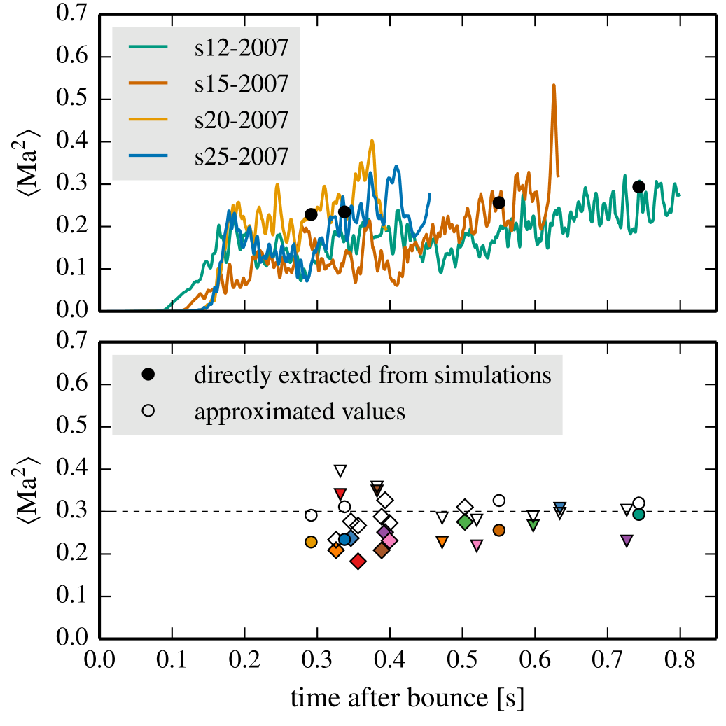
Figure 13.— In the upper panel, the time evolution of the average squared Mach number in the gain layer (calculated without approximation) is shown for the simulations of Model Set I. The curves in the upper panel are smoothed by running averages of 5 ms. In the bottom panel, the average squared Mach number (cf. Eq. 21) is given for all 18 models at the time when the ratio $\tau_{\mathrm{adv}}/\tau_{\mathrm{heat}}$ reaches unity. Filled symbols indicate the values directly evaluated from the simulations, empty symbols denote the approximation given by Equations (41) and (52) of Müller & Janka (2015). The dashed line indicates the critical limit suggested by Müller & Janka (2015).

Although the time-scale criterion appears to be a reliable concept for the description of the explosion behavior in all 18 axisymmetric simulations (in a post-dictive, diagnostic manner), at first glance no obvious correlations with other characteristic quantities can be found that point to generally valid properties at the onset of the explosion. At the time the ratio $\tau_{\mathrm{adv}}/\tau_{\mathrm{heat}}$ reaches unity, the models exhibit a diverse range of average and maximum shock radii, neutrino luminosities and mean energies, kinetic energies and fractions of recombined matter in the gain layer, etc. (see, for example, Tab. 1 and Figs. 2 to 6), and the conditions necessary for shock revival do not seem to be constrained tightly enough to define a common framework for a successful runaway.

Müller & Janka (2015) suggest that in 2D a squared turbulent Mach number of $\langle\mathrm{Ma}^{2}\rangle\gtrsim 0.3$ is needed for runaway. The average squared Mach number of the turbulent lateral motions in the gain region is defined as

$$\langle\mathrm{Ma}^{2}\rangle=\frac{\langle v_{\theta}^{2}\rangle}{\langle c_{\mathrm{s,g}}^{2}\rangle}=\frac{2E_{\mathrm{kin,g}}^{\mathrm{lat}}/M_{\mathrm{g}}}{\langle c_{\mathrm{s,g}}^{2}\rangle}.$$ (21)

In contrast to Müller & Janka (2015), we do not employ further approximations for the sound speed $c_{\mathrm{s,g}}$, but extract all quantities directly from the numerical simulations as mass-weighted averages over the gain layer instead of quantities measured behind the shock:

$$\langle c_{\mathrm{s,g}}^{2}\rangle=\frac{1}{M_{\mathrm{g}}}\int\limits_{R_{\mathrm{g}}(\theta)<r<R_{\mathrm{s}}(\theta)}c_{\mathrm{s}}^{2}\rho\,\mathrm{d}V.$$ (22)

The consequences of the two different approaches concerning the determination of $c_{\mathrm{s,g}}$ can be inferred from Fig. 13, where the time evolution of the average squared Mach number for Model Set I is shown (calculated without approximation, see upper panel) and the average squared Mach numbers of all 18 models are given at the time the ratio $\tau_{\mathrm{adv}}/\tau_{\mathrm{heat}}$ reaches unity (calculated with and without approximation, see lower panel). The time scales $\tau_{\mathrm{adv}}$ and $\tau_{\mathrm{heat}}$ are calculated according to Eqs. (4) and (6). While the approximate calculation of $\langle\mathrm{Ma}^{2}\rangle$ only takes into account post-shock quantities with a number of simplifying assumptions (see Müller & Janka, 2015), the direct calculation considers the (averaged) properties of the whole gain region, because such an analysis offers more numerical robustness than a calculation directly behind the shock. The latter approach typically results in smaller Mach numbers (compare empty and filled circles in the lower panel of Fig. 13), and the correlation between Mach number and the onset of explosion (defined by $\tau_{\mathrm{adv}}/\tau_{\mathrm{heat}}=1$) points towards a ‘critical squared Mach number’ around $\sim 0.25$ and thus below the value of 0.3 found by Müller & Janka (2015). However, there are considerable temporary fluctuations in which $\langle\mathrm{Ma}^{2}\rangle$ can exceed the value of 0.25 for transient times even before shock runaway occurs. Moreover, at the time when $\tau_{\mathrm{adv}}/\tau_{\mathrm{heat}}\sim 1$, the individual values scatter by more than $\sim 30\,\%$ around the mean critical value of all models, for which reason the turbulent Mach number is at most indicative, but has no hard threshold for shock runaway. This suggests a considerable model-to-model variation of the turbulent pressure contribution, being only one of several elements that play a role in triggering the explosion.

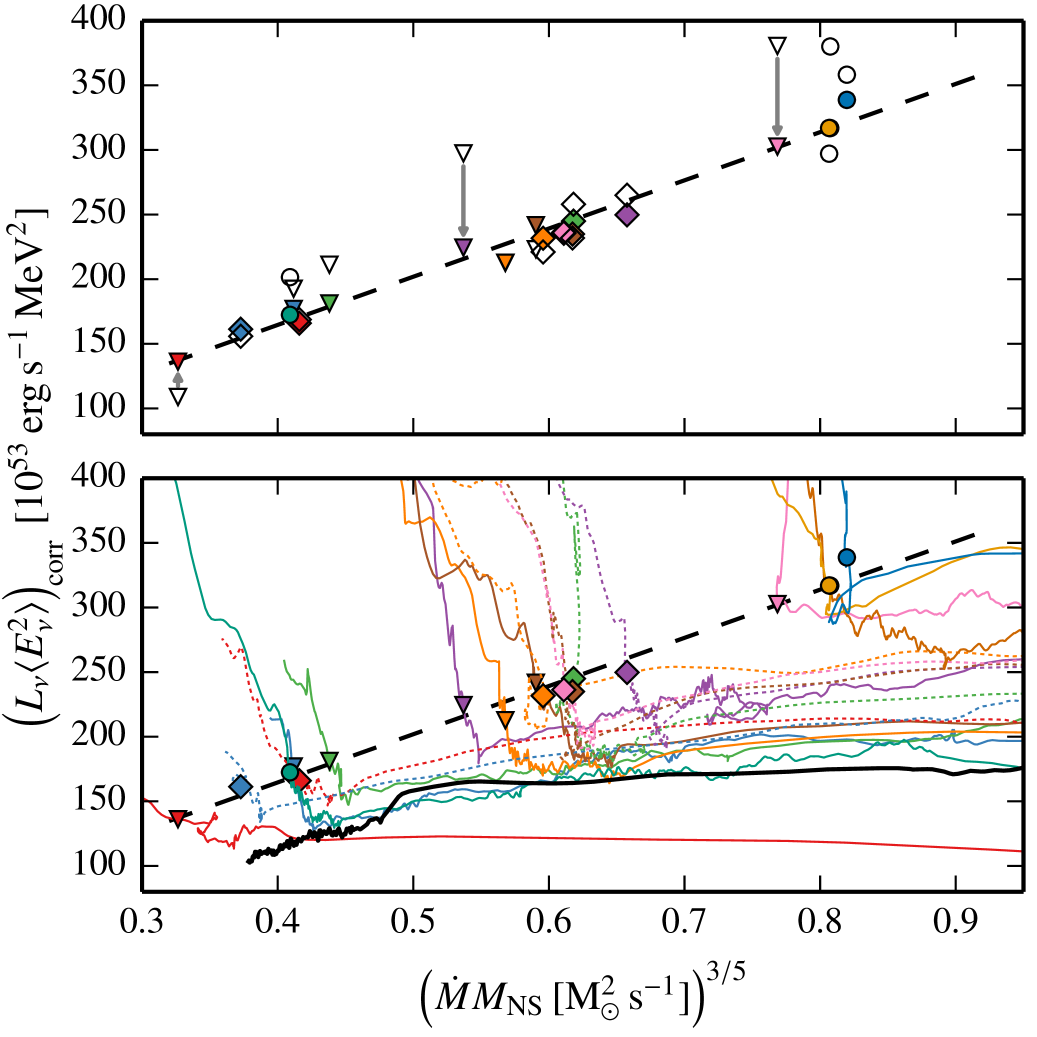
Figure 14.— Critical luminosity condition for explosion. In both panels, the critical relation between $\left(L_{\nu}\langle E_{\nu}^{2}\rangle\right)_{\mathrm{corr}}$ and $\left(\dot{M}M_{\mathrm{NS}}\right)^{3/5}$ for the onset of explosion (see Eqs. 32 and 34) is depicted as black dashed line obtained from a least-squares fit to the critical points of all 18 axisymmetric models. The symbols indicate these critical points corresponding to the time when the ratio $\tau_{\mathrm{adv}}/\tau_{\mathrm{heat}}$ reaches unity. Circles denote the models of Set I, and triangles (diamonds) indicate the models of Set II with lower (higher) ZAMS masses following the classification and color coding used in previous figures. In the upper panel, a comparison between corrected (filled symbols) and uncorrected (empty symbols) values of the critical luminosity is shown. In three exemplary cases, the shifts introduced by the correction factor are indicated by gray arrows. In the lower panel, the trajectories of all 18 models in the $\left(L_{\nu}\langle E_{\nu}^{2}\rangle\right)_{\mathrm{corr}}$-$\left(\dot{M}M_{\mathrm{NS}}\right)^{3/5}$ plane for corrected values are additionally given (models of Set II with higher ZAMS masses are shown with dotted lines). Furthermore, an axisymmetric (2D) $15\,\mathrm{M}_{\odot}$ model of Heger et al. (2005) that does not evolve towards an explosion is depicted with a black solid line. All depicted values are smoothed by running averages of 25 ms.

In principle, it is possible to relate the ‘critical luminosity’ (Burrows & Goshy, 1993; Murphy & Burrows, 2008; Pejcha & Thompson, 2012) that is required to overcome the ram pressure at a given mass-accretion rate to the time-scale criterion $\tau_{\mathrm{adv}}/\tau_{\mathrm{heat}}\gtrsim 1$ (cf. Janka, 2012). But in contrast to studies in spherical symmetry, non-radial instabilities in multidimensional simulations play a crucial role for the supernova explosion mechanism and directly influence the critical luminosity condition. While theories have been proposed to describe the saturation properties of the SASI (e.g. Guilet et al., 2010) and of convection (e.g. Murphy & Meakin, 2011; Murphy et al., 2013), only few works focused on a simplification of these theories to scaling laws that can be easily verified by the extraction of volume-integrated quantities from multidimensional simulations. Murphy et al. (2013) performed a quantitative analysis of the interdependence of neutrino heating and non-radial instabilities with respect to the effect of turbulent motions on the average shock radius. In Müller & Janka (2015), semi-empirical scaling laws were formulated that describe the relations between the turbulent kinetic energy and Mach number, shock deformation, and neutrino heating. In the following, guided by the results of Müller & Janka (2015), we aim at investigating to what extent the additional consideration of turbulent stresses in the gain layer can lead to a generalizable description of the explosion conditions, being commonly applicable to all 18 simulations.

In order to derive the critical luminosity, we start with the spherical symmetric case, considering the scaling relations for $\tau_{\mathrm{adv}}$,

$$\tau_{\mathrm{adv}}\propto\frac{R_{\mathrm{s}}^{3/2}}{\sqrt{M_{\mathrm{NS}}}},$$ (23)

and $\tau_{\mathrm{heat}}$,

$$\tau_{\mathrm{heat}}\propto\frac{\left|\bar{e}_{\mathrm{tot,g}}\right|R_{\mathrm{g}}^{2}}{L_{\nu}\langle E_{\nu}^{2}\rangle}$$ (24)

(see Janka, 2012). Here, $\bar{e}_{\mathrm{tot,g}}$ is the average mass-specific binding energy in the gain layer:

$$\bar{e}_{\mathrm{tot,g}}=\frac{E_{\mathrm{tot,g}}}{M_{\mathrm{g}}},$$ (25)

where $E_{\mathrm{tot,g}}$ is defined in Eq. (7). $L_{\nu}$ is defined as the total luminosity $L_{\nu}=L_{\nu_{\mathrm{e}}}+L_{\bar{\nu}_{\mathrm{e}}}$ of $\nu_{\mathrm{e}}$ and $\bar{\nu}_{\mathrm{e}}$, and $\langle E_{\nu}^{2}\rangle$ denotes the weighted average of the mean squared energies of electron neutrinos and antineutrinos:

$$\langle E_{\nu}^{2}\rangle=\frac{L_{\nu_{\mathrm{e}}}\langle E_{\nu_{\mathrm{e}}}^{2}\rangle+L_{\bar{\nu}_{\mathrm{e}}}\langle E_{\bar{\nu}_{\mathrm{e}}}^{2}\rangle}{L_{\nu_{\mathrm{e}}}+L_{\bar{\nu}_{\mathrm{e}}}}.$$ (26)

As in Eq. (10), the mean squared energies are defined as $\langle E_{\nu_{\mathrm{e}}}^{2}\rangle\coloneqq\langle\epsilon_{\nu_{\mathrm{e}}}^{3}\rangle/\langle\epsilon_{\nu_{\mathrm{e}}}\rangle$ and $\langle E_{\bar{\nu}_{\mathrm{e}}}^{2}\rangle\coloneqq\langle\epsilon_{\bar{\nu}_{\mathrm{e}}}^{3}\rangle/\langle\epsilon_{\bar{\nu}_{\mathrm{e}}}\rangle$. According to Janka (2012), the shock radius in spherical symmetry follows the relation

$$R_{\mathrm{s}}\propto\frac{\left(L_{\nu}\langle E_{\nu}^{2}\rangle\right)^{4/9}R_{\mathrm{g}}^{16/9}}{\dot{M}^{2/3}M_{\mathrm{NS}}^{1/3}}.$$ (27)

By the use of these approximate scaling relations, the time-scale criterion $\tau_{\mathrm{adv}}/\tau_{\mathrm{heat}}\sim 1$ can be translated into a critical luminosity condition which depends on the mass-accretion rate, the proto-neutron star mass, the gain radius, and the average specific binding energy in the gain layer:

$$\left(L_{\nu}\langle E_{\nu}^{2}\rangle\right)_{\mathrm{crit}}\propto\left(\dot{M}M_{\mathrm{NS}}\right)^{3/5}\left|\bar{e}_{\mathrm{tot,g}}\right|^{3/5}R_{\mathrm{g}}^{-2/5}.$$ (28)

Note that we do not omit $\bar{e}_{\mathrm{tot,g}}$ and $R_{\mathrm{g}}$ in this relation.

For the multidimensional case, we follow Müller & Janka (2015) and consider the turbulent stresses of multidimensional flows in the gain layer by introducing an additional isotropic pressure contribution $P_{\mathrm{turb}}\approx\langle\delta v^{2}\rangle\rho\approx 4/3\langle\mathrm{Ma}^{2}\rangle P$. The consideration of this additional post-shock pressure leads to an increased advection time scale because of a larger radius of the stalled shock compared to Eq. (27):

$$R_{\mathrm{s}}\propto\frac{\left(L_{\nu}\langle E_{\nu}^{2}\rangle\right)^{4/9}R_{\mathrm{g}}^{16/9}}{\dot{M}^{2/3}M_{\mathrm{NS}}^{1/3}}\left(1+\frac{4\langle\mathrm{Ma}^{2}\rangle}{3}\right)^{2/3}$$ (29)

(see Appendix B of Müller & Janka, 2015). Taking this modification into account, the scaling relation for the critical luminosity now reads

$$\left(L_{\nu}\langle E_{\nu}^{2}\rangle\right)_{\mathrm{crit}}\propto\left(\dot{M}M_{\mathrm{NS}}\right)^{3/5}\xi_{\mathrm{g}},$$ (30)

where the time dependent quantity $\xi_{\mathrm{g}}$ subsumes all gain-layer related properties:

$$\xi_{\mathrm{g}}\coloneqq\left|\bar{e}_{\mathrm{tot,g}}\right|^{3/5}R_{\mathrm{g}}^{-2/5}\left(1+\frac{4\langle\mathrm{Ma}^{2}\rangle}{3}\right)^{-3/5}.$$ (31)

$\xi_{\mathrm{g}}$ can be used to correct $L_{\nu}\langle E_{\nu}^{2}\rangle$ with respect to the time-dependent evolution of gain radius, binding energy, and turbulent pressure in the gain layer, which lead to a time and model dependence of the critical luminosity condition for an explosion in addition to its dependence on $M_{\mathrm{NS}}$ and $\dot{M}$:

$$\left(L_{\nu}\langle E_{\nu}^{2}\rangle\right)_{\mathrm{crit,corr}}\coloneqq\frac{1}{\xi_{\mathrm{g}}/\xi_{\mathrm{g}}^{*}}\left(L_{\nu}\langle E_{\nu}^{2}\rangle\right)_{\mathrm{crit}}.$$ (32)

In order to obtain a meaningful comparison between different models, we also introduce a constant normalization factor $\xi_{\mathrm{g}}^{*}$ such that the correction is applied relative to a reference model. This reference model can be chosen arbitrarily. For our analysis we selected model s16.8 and evaluated $\xi_{\mathrm{g}}^{*}$ at the time when the ratio $\tau_{\mathrm{adv}}/\tau_{\mathrm{heat}}$ reaches unity:

$$\xi_{\mathrm{g}}^{*}\coloneqq\left.\left|\bar{e}_{\mathrm{tot,g}}\right|^{3/5}R_{\mathrm{g}}^{-2/5}\left(1+\frac{4\langle\mathrm{Ma}^{2}\rangle}{3}\right)^{-3/5}\right|^{\mathrm{s16.8}}_{\tau_{\mathrm{adv}}/\tau_{\mathrm{heat}}=1}.$$ (33)

This, finally, leads to a generalized version of the critical condition, now applying to the corrected values of $L_{\nu}\langle E_{\nu}^{2}\rangle$:

$$\left(L_{\nu}\langle E_{\nu}^{2}\rangle\right)_{\mathrm{crit,corr}}\propto\left(\dot{M}M_{\mathrm{NS}}\right)^{3/5}.$$ (34)

The results of our analysis are shown in Fig. 14, the corresponding correction factors are given in Table 2. In addition to the time evolution of the corrected and normalized values of $\left(L_{\nu}\langle E_{\nu}^{2}\rangle\right)_{\mathrm{corr}}=\left(\xi_{\mathrm{g}}/\xi_{\mathrm{g}}^{*}\right)^{-1}\left(L_{\nu}\langle E_{\nu}^{2}\rangle\right)$ versus $\left(\dot{M}M_{\mathrm{NS}}\right)^{3/5}$ (lower panel), we depict the instants when the ratio $\tau_{\mathrm{adv}}/\tau_{\mathrm{heat}}$ exceeds unity. In the upper panel, these points are shown with corrections (filled symbols) and without corrections (empty symbols). The success of the correction procedure is evident: accounting for the additional dependence of the critical luminosity condition on $\bar{e}_{\mathrm{tot,g}}$, $R_{\mathrm{g}}$, and in particular on the turbulent stresses of multidimensional flows in the gain layer leads to the expected strong correlation with $\dot{M}M_{\mathrm{NS}}$, and a generalized critical curve (indicated by the black dashed line) appears which is valid for all 18 explosion models. Note that the critical curve shows up as a straight line in Fig. 14 since we plot $\left(\dot{M}M_{\mathrm{NS}}\right)^{3/5}$ on the abscissa. All models approach the critical curve from the right and move upwards after reaching the critical condition. The upward bending of the evolutionary tracks at the onset of explosion is caused by a steep drop of $\xi_{\mathrm{g}}$ in the denominator while $\left(L_{\nu}\langle E_{\nu}^{2}\rangle\right)$ in the numerator evolves slowly. The decline of $\xi_{\mathrm{g}}$ occurs because an increase of $\left(1+4/3\langle\mathrm{Ma}^{2}\rangle\right)$ supports the outward acceleration of the shock and, as a consequence, the specific binding energy of the gain layer, $\left|\bar{e}_{\mathrm{tot,g}}\right|$, plummets in addition. Interestingly, also the behavior of the models exploding at rather late times after bounce is correctly captured by this condition. This further underlines the general validity of the critical curve defined above.

In view of the analysis of Radice et al. (2016), which demonstrates that aside of the turbulent pressure other effects of turbulence, e.g. a term associated with centrifugal support, play an equally important role, it is quite astonishing that a simple correction by the turbulent pressure term in the critical luminosity condition seems to capture the overall effects of multidimensional fluid motions in the gain layer remarkably well.

For comparison, we also show the trajectory of a model from Heger et al. (2005) (m15b6, simulated in axisymmetry (2D) without the consideration of rotational effects) that does not explode. As indicated by the solid black line in the lower panel of Fig. 14, this model does not reach the critical luminosity condition, but evolves in parallel to the critical curve in downward direction. The fact that this model does not fulfill the necessary condition for a successful runaway is correctly mirrored by its time evolution in the $\left(L_{\nu}\langle E_{\nu}^{2}\rangle\right)_{\mathrm{corr}}-\left(\dot{M}M_{\mathrm{NS}}\right)^{3/5}$ plane (Eqs. 31-34). In summary, the critical curve constructed as described above proves to be an excellent yardstick for the onset of the explosion and defines a reliable, general criterion for the development of runaway conditions in the simulations.

5. Conclusions

Our study of 18 pre-supernova models in a range of 11 to 28 solar masses, using 2D simulations with three-flavor, energy dependent, ray-by-ray-plus neutrino transport including the full set of state-of-the-art neutrino reactions and microphysics, underlines the viability of the neutrino-driven mechanism in axisymmetry. All investigated models explode and a systematic comparison of the model set shows that the explosions are strongly influenced by the pre-collapse structure of the progenitor star.

If the progenitor exhibits a pronounced decline of the density at the Si/Si-O composition shell interface, the rapid drop of the mass-accretion rate at the time when the interface arrives at the shock front induces a steep reduction of the accretion ram pressure. This causes a strong shock expansion supported by neutrino heating and thus favors an early explosion. Such a behavior is particularly likely when the mass-accretion rate is high before the Si/Si-O interface passes the shock. In this case the neutron star mass grows quickly and a high accretion luminosity ensures a high neutrino heating rate even after the composition-shell interface has fallen through the shock. If the progenitor structure does not exhibit a pronounced density jump at the Si/Si-O interface and the mass-accretion rate decreases more slowly, the models tend to explode rather late when the mass-accretion rate has declined enough for the neutrino heating to overcome the accretion ram pressure.

Due to initially rather short advection time scales, our simulations provide favorable conditions for the efficient growth of the SASI. Large-scale mass motions in the post-shock layer associated with low-mode oscillations of the supernova shock front along the symmetry axis mirror the vivid SASI activity in our models, and the final shock expansion is initiated by the growth of large bubbles supported by this instability. But also the strong influence of convection is visible: When the time-scale ratio approaches unity, the $\chi$ parameter increases above the critical value of 3. A comparison to the SASI and convection dominated models discussed by Fernández et al. (2014) confirms the typical fingerprints of both convection and the SASI in our models, since the turbulent energy spectra of our simulations show the characteristic SASI peak at a spherical harmonics mode of $l=2$ as well as enhanced convective power at higher modes of $l=5-10$.

Table 2Correction factors for the critical luminosity
used in Eq. (32)

model	$(\xi_{\mathrm{g}}/\xi_{\mathrm{g}}^{*})^{-1}$	model	$(\xi_{\mathrm{g}}/\xi_{\mathrm{g}}^{*})^{-1}$
Model Set I		Model Set II
s12-2007	0.86	s11.2	1.25
s15-2007	0.83	s12.4	0.92
s20-2007	1.07	s13.2	0.86
s25-2007	0.95	s14.4	0.75
		s16.8	1.00
		s17.2	1.08
		s18.4	0.80
		s19.6	0.98
		s20.2	1.04
		s21.6	0.95
		s22.4	0.94
		s26.6	1.05
		s27.0	1.01
		s28.0	1.00

Note. — $\xi_{\mathrm{g}}$ and $\xi_{\mathrm{g}}^{*}$ are defined in Eqs. (31) and (33).

The investigation of a larger set of self-consistent CCSN simulations naturally leads to the question of common properties shared by all models that govern the onset of the successful explosions. Although the time-scale criterion proves to be a reliable diagnostic parameter for runaway, obvious correlations with specific values of other variables discussed in Sect. 3 cannot be found. Following the approach suggested by Müller & Janka (2015) to account for the role of non-radial instabilities in the concept of a critical neutrino luminosity for the onset of neutrino-driven explosions, we generalize the critical luminosity relation by including corrections for the effects of turbulent stresses (and of other time-dependent parameters) in the gain layer (see Eqs. 31-34). This relation defines a direct proportionality between the corrected product of $\left(L_{\nu}\langle E_{\nu}^{2}\rangle\right)_{\mathrm{corr}}$ and $\left(\dot{M}M_{\mathrm{NS}}\right)^{3/5}$ and captures the explosion behavior of all 18 models in an excellent way, thus reliably determining the conditions necessary for the onset of the runaway. Our $\left(L_{\nu}\langle E_{\nu}^{2}\rangle\right)_{\mathrm{corr}}-\dot{M}M_{\mathrm{NS}}$ relation (see Eq. (34) and Fig. 14) leads to a considerable reduction of the scattering of the critical runaway condition of all models compared to the uncorrected case as well as compared to the $L_{\nu}-\dot{M}$ condition discussed by Suwa et al. (2016), see Figure 18 there.

Since recent 2D core-collapse simulations by Bruenn et al. (2013, 2016), Dolence et al. (2015), O’Connor & Couch (2015), and Skinner et al. (2015) focused on four progenitors models of Woosley & Heger (2007) that are extensively investigated also in this work, detailed comparisons between different codes applied to the CCSN problem become possible now. At first glance, the differences between the results give reasons for concern (for a cautious effort of a comparative discussion see also Janka et al., 2016): the same progenitor models fail to explode (e.g. Dolence et al., 2015, but with Newtonian gravity and different EoS), explode very early at a time that is nearly independent of the progenitor mass (e.g. Bruenn et al., 2013, 2016), or explode later, showing a strong influence of the respective progenitor structure (this work). However, O’Connor & Couch (2015) demonstrated that Newtonian gravity (as applied by Dolence et al., 2015) is not favorable for explosions while a relativistic potential is. Skinner et al. (2015) reported differences in the dynamical evolution of the four progenitor models with M1 and ray-by-ray neutrino transport, the latter favoring explosions. But these results are in conflict with the M1 models of O’Connor & Couch (2015), which show overall agreement with the ray-by-ray-plus results presented in our work. Curiously, the differences observed by Skinner et al. (2015) decreased when the resolution of their simulations was enhanced. Good overall agreement with our results was also demonstrated in a recent conference talk at FOE2015 by K. Kotake, who presented his simulations for a subset of cases of our Model Set II.

A profound analysis of similarities and differences of simulations depending on the applied codes and microphysics is demanded to shed light on the sensitivity of the CCSN dynamics to the approximations still used in current simulations. Particular attention will have to be paid to the possible role of code- and method inherent numerical perturbations, which might foster the growth of post-shock instabilities and could have important consequences for the onset of explosions (Couch & Ott, 2013, 2015; Müller & Janka, 2015). A close comparison will help putting present CCSN simulations on a touchstone and will point to necessary improvements in the modeling of this important astrophysical problem.

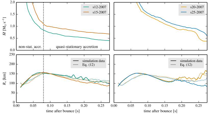
Figure 15.— Mass-accretion rates (top panels) and mean shock trajectories (bottom panels) for the models of Set I with the lower-mass cases on the left and the higher-mass cases on the right. In the lower panels, solid lines denote the simulation data, while the dotted lines provide the analytic approximation of Eq. (12). The latter holds for quasi-stationary accretion conditions, which apply better in the low-mass cases after an initial phase of high mass-accretion rates. In the high-mass models, the accretion rates continue to remain on a high level with a steep decline for a longer period of time, for which reason the analytic approximation roughly captures the general trend but does not show the good quality of the quantitative agreement visible in the lower left panel.

The following appendices provide information on several aspects of discussion in detail. First, we demonstrate the viability of Eq. (12) for a rough description of the steady-state evolution of the radius of the accretion shock. Second, we follow Nakamura et al. (2015) and present correlations of some explosion properties with the compactness parameter $\xi_{2.0}$ defined by Eq. (1).

Moreover, we aim at studying the resolution and stochasticity dependence of our results with respect to the point in time when the explosion sets in. This is intended to further validate the connection between progenitor structure and post-bounce evolution that is evident in our simulations and has been extensively discussed in this paper. We also vary the chosen transition density between the high- and the low-density EoS and study the influence of different treatments of energy conservation on the simulation outcome.

In addition, we will test the effects of differences in the employed neutrino physics compared to the models of Bruenn et al. (2013, 2016) on the shock and neutron star radii. Even in 1D, these quantities differ significantly between the simulation results of Prometheus-Vertex and the published results of the Chimera code used by the Oak Ridge group. We note, however, that the Oak Ridge group has recently presented 1D results for “Series C” models (Lentz et al., 2015), where the shock radii are considerably smaller than in the previous “Series B” 1D models of Bruenn et al. (2013, 2016), and therefore closer to our results obtained with Prometheus-Vertex.

We emphasize that our multidimensional code retains spherical symmetry exactly if no seed perturbations are applied. Despite their potentially important role for the development of post-shock instabilities (Couch & Ott, 2013, 2015; Müller & Janka, 2015), we have not varied the recipe of random seeds employed in this study but have constrained ourselves to the seeding method described in Sect. 2 for all models.

Appendix A Evolution of mean shock radius and analytic approximation

In order to demonstrate the viability of Eq. (12) for a rough description of the time evolution of the mean shock radius, Fig. 15 displays the shock trajectories for the four models of our Set I. Both the simulation data (solid lines) and the proportionality relation according to Eq. (12) (dotted lines; the normalization constant of this relation is chosen such that the relation matches the simulation data at 0.1 s) are shown. Eq. (12) describes the simulation data very closely only in a time interval in which steady-state conditions are roughly fulfilled. This is the case after the early maximum of the shock expansion (the initial shock expansion is driven by the non-stationary accumulation of an accretion mantle around the neutron star) and before the development of strong non-radial mass motions in the post-shock flow. A steep decline of the mass-accretion rate continues for a longer period of time in the two more massive models, while the two less massive cases reach a quasi-stationary accretion state after about 80 ms of post-bounce evolution (see top row of Fig. 15). Therefore the requirement of stationarity is better fulfilled for the two less massive stars, for which reason the proportionality relation of Eq. (12) agrees better with the simulation data. Since the low-mass cases explode only late, their early conditions are farther away from the threshold to explosion and multidimensional effects play a minor role, whereas such effects are slightly more visible in the two more massive models.

Appendix B Explosion properties and compactness parameter

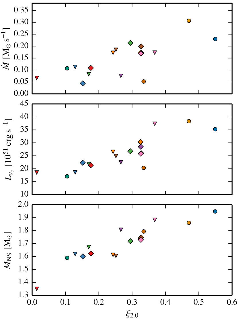
Figure 16.— Mass-accretion rate, electron neutrino luminosity, and proto-neutron star mass as functions of the compactness parameter $\xi_{2.0}$ (from top to bottom). Following Nakamura et al. (2015), the proto-neutron star mass is given at the final time of the simulation, the two other quantities are evaluated at the time when the mean shock radius reaches 400 km. Circles denote the models of Set I, and triangles (diamonds) indicate the models of Set II with lower (higher) ZAMS masses in line with the classification and color coding used in previous figures.

In Fig. 16, the mass-accretion rate, $\dot{M}$, the electron neutrino luminosity, $L_{\nu_{\mathrm{e}}}$, and the mass of the proto-neutron star, $M_{\mathrm{NS}}$, are shown for our 18 explosion models as functions of the compactness parameter $\xi_{2.0}$ (cf. Eq. 1). As in Table 1, the compactness parameter is calculated from the pre-supernova model (which in this case is identical to the value at bounce). Following Nakamura et al. (2015), $\dot{M}$ and $L_{\nu_{\mathrm{e}}}$ (as defined in Sect. 3.1.1) are evaluated at the time when the mean shock radius reaches a value of 400 km, while $M_{\mathrm{NS}}$ is given at the final time of our simulations. We constrain the cases of Fig. 16 to a single value of $\xi_{M}$ (different from Nakamura et al., 2015), since choices of $1.5\lesssim M\lesssim 2.5$ show similar correlations. Although our model set exhibits the same increasing trends found by Nakamura et al. (2015), only 18 data points do not provide sufficient statistics for a meaningful derivation of correlations. The observed trends can also be expected for fundamental physical reasons and are therefore not astonishing: For models with a higher compactness parameter $\xi_{2.0}$, the mass coordinate of $2.0\,\mathrm{M}_{\odot}$ is located at a smaller radius $R(M=2.0\,\mathrm{M}_{\odot})$ than for models with lower compactness. The same mass being compressed into a smaller sphere of radius $R(M=2.0\,\mathrm{M}_{\odot})$ then translates into a longer-lasting high mass-accretion rate (Fig. 16, top panel), leading to a higher accretion luminosity (Fig. 16, middle panel) and to a higher proto-neutron star mass (Fig. 16, bottom panel). But we would also like to underline that, despite of the overall rough trends, the significant scatter of the depicted quantities points towards peculiar model characteristics which cannot be captured sufficiently well by a single parameter like the compactness. As discussed and demonstrated in Sect. 4, the formulation of a criterion that reliably determines the development of runaway conditions in multidimensional simulations especially requires a proper consideration of the model-dependent effects of non-radial mass motions.

Appendix C Resolution Dependence and Stochasticity of the Results

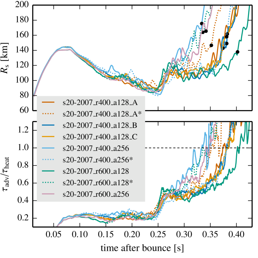
Figure 17.— Time evolution of shock radius (upper panel) and time-scale ratio (lower panel) for a set of nine 2D simulations for the same progenitor model, but with different angular and radial resolutions and with different random perturbations for seeding non-radial hydrodynamic instabilities. The black dots in the top panel mark the point in time when the ratio $\tau_{\mathrm{adv}}/\tau_{\mathrm{heat}}$ reaches unity. All quantities are angle-averaged and the curves are smoothed by running averages of 5 ms.

For the resolution study, we chose model s20-2007 of Woosley & Heger (2007). The setups of the simulations are listed in Table  3. Besides two different angular resolutions of 128 and 256 angular zones, radial grids of initially 400 and 600 zones (both gradually further refined during the simulations) were used, and various combinations of the highly and moderately resolved angular and radial grids were tested. We also varied the random seeds (but without changing the seeding recipe) for the density perturbations introduced 10 ms after bounce (compare model s20-2007_r400_a128_A, s20-2007_r400_a128_B, and s20-2007_r400_a128_C). This affects only the perturbation pattern, the perturbation amplitude of 0.1 % in density was the same for all models. In order to test for the stochasticity of the results, the models with names appended by an asterisk are just a repetition of the simulations without asterisk for the same initial conditions (i.e., also the same perturbations).

The numerical setup of the models was identical to the description in Sect. 2 except for several code improvements that were only used in the simulations of this section. Besides minor changes this includes a more sophisticated treatment of total energy conservation (cf. Müller et al., 2010) and the correction of an erroneously applied identity of the charged-current neutrino absorption coefficient in eight-cell OpenMP patches. While the latter improvement has no noticeable effects on the results of test calculations, the improved treatment of the total energy conservation leads to slightly smaller shock radii at earlier times ($\Delta R_{\mathrm{s}}\lesssim 10\,\mathrm{km}$ at the time of maximal shock expansion, $R_{\mathrm{s,max}}\sim 150\,\mathrm{km}$), and we observe a somewhat delayed ($\sim 70\,\mathrm{ms}-100\,\mathrm{ms}$) development of a runaway situation compared to the s20-2007 case presented in Sect. 3 (compare Figs. 17 and 2). But as we will show in the following, stochasticity seems to be the key determinant for the exact timing of the onset of explosion.

Since the hydrodynamic flow behind the shock front evolves highly non-linearly and in a chaotic way, differences in the detailed post-bounce dynamics of the presented simulations are expected, even if initial conditions and grid resolutions are identical. After 150 ms, this can be observed in the evolution of the shock radius and the time-scale ratio of models s20-2007_r400_a128_A and s20-2007_r400_a128_A* shown in Fig. 17. The stochastic nature of the developing non-radial flow in the post-shock layer results in a difference of $\sim 30\,\mathrm{ms}$ between the times when the critical condition $\tau_{\mathrm{adv}}/\tau_{\mathrm{heat}}\gtrsim 1$ is reached (see Fig. 17). Similar stochastic differences can be observed for the models with higher resolution (compare the time evolution of models s20-2007_r600_a128 with s20-2007_r600_a128* or s20-2007_r400_a256 with s20-2007_r400_a256*). It is remarkable that not even in the case of the same initial conditions our simulations completely agree in the details of their time evolution. This can be explained by the applied compiler optimizations which are chosen to enhance the code performance, but also marginally influence the precision of floating-point operations. Further enhanced by the turbulent, non-linear evolution of the hydrodynamic dynamics behind the shock, these minimal differences can lead to a certain spread in the evolution of the models.

Models with a higher angular resolution of 256 zones seem to show a trend towards a slightly earlier runaway than the simulations with 128 angular zones. This is in accordance with the results of Hanke et al. (2012) and their set of simulations using only a simplified and parametrized neutrino treatment. However, the rather small difference in time when the critical condition is met compared to models s20-2007_r400_a128_A* and s20-2007_r600_a128*, which show the earliest runaway of all models with lower angular resolution, again suggests stochastics as likely main reason for the observed differences between the models. This is also the case for the models with initially higher radial resolution: Only differences of the order of a few tens of milliseconds can be observed concerning the points in time when the runaway sets in.

Table 3Tests of resolution and EoS treatment

model	# of radial zones	# of angular zones
Resolution tests:
s20-2007_r400_a128_A	400	128
s20-2007_r400_a128_A*	400	128
s20-2007_r400_a128_B	400	128
s20-2007_r400_a128_C	400	128
s20-2007_r400_a256	400	256
s20-2007_r400_a256*	400	256
s20-2007_r600_a128	600	128
s20-2007_r600_a128*	600	128
s20-2007_r600_a256	600	256
Transition density tests:
s20-2007_r400_a88_rho3.4e7	400	88
s20-2007_r400_a88_rho6.0e7	400	88
s20-2007_r400_a88_rho3.0e8	400	88

Note. — Naming convention: numerical values following the small letters ‘r’ and ‘a’ indicate the numbers of radial and angular grid cells, respectively. Capital letters A, B, and C at the end of the model name denote different patterns of density perturbations imposed 10 ms after bounce. Models with an asterisk are just a repetition of the models without asterisk with the same initial conditions. In the cases of the tests for the EoS transition density, the respective density values are also given. In all resolution tests, a transition density of $3.0\times 10^{8}\mathrm{g\,cm}^{-3}$ was applied.

In a similar resolution study performed by Hanke (2014) for model s27.0, higher angular resolution hardly made any difference for the simulation results, whereas higher radial resolution (combined with high angular resolution) led to a delay of the runaway. While our study also shows a delay in the case of model s20-2007_r600_a128, where only the radial resolution was increased, our two models with enhanced angular and enhanced angular and radial resolution, respectively, explode rather early. This is also the case for model s20-2007_r600_a128*. The fact that the resolution changes do not produce uniform results again underlines the strong influence of stochastic turbulent motions on the onset of explosion.

Overall, the results of our resolution study can be summarized as follows. Although the time difference between the simulation showing the earliest runaway and the simulation exploding latest amounts to $\sim 80\,\mathrm{ms}$ (defined by the point in time when the critical time-scale ratio is reached), the development of the explosion is mainly triggered by the arrival of the Si/Si-O composition shell interface at the shock. When the ram pressure of the infalling material is reduced to such an extent that neutrino heating can revive the shock, the explosion is initiated. The associated development of turbulent motions due to convection and the SASI promotes the shock revival by increasing the dwell time of matter in the gain layer and additional support of the shock by turbulent momentum flows and pressure, and the stochasticity of these fluid motions finally leads to the moderate variance regarding the further evolution of the explosion. Different patterns of initial density perturbations or an energy cascade better resolved by a higher number of grid zones affect the evolution of the turbulent motions, but according to our resolution study, these are only secondary effects. This underlines the validity of our conclusions regarding the strong connection between post-bounce evolution and pre-collapse structure as evident in the results presented in the main text of our paper.

Appendix D Influence of pre-bounce EoS transition density

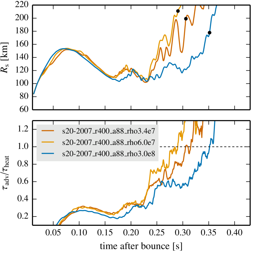
Figure 18.— Time evolution of shock radius (upper panel) and time-scale ratio (lower panel) for a set of three 2D simulations for the same progenitor model, but with different choices for the transition density between the high- and the low-density EoS before bounce. The black dots in the top panel mark the point in time when the ratio $\tau_{\mathrm{adv}}/\tau_{\mathrm{heat}}$ reaches unity. All quantities are angle-averaged and the curves are smoothed by running averages of 5 ms.

In addition to the tests of resolution and stochastic effects, we also varied the choice of the density at which the transition from the high-density to the low-density EoS is placed (cf. Rampp & Janka, 2002; Buras et al., 2006a). During the collapse phase until core bounce, the values for the transition density were chosen to be $3.4\times 10^{7}\,\mathrm{g\,cm}^{-3}$, $6.0\times 10^{7}\,\mathrm{g\,cm}^{-3}$, and $3.0\times 10^{8}\,\mathrm{g\,cm}^{-3}$, respectively (see Table 3 and Fig. 18). The last value was the one used in all 18 simulations presented in Sect. 3. In the post-bounce phase the transition density was moved to $10^{11}\,\mathrm{g\,cm}^{-3}$ in all cases, because below this density nucleon interactions play a negligible role and our low-density NSE solver allows for the consideration of a larger set of nuclear species during the expansion phase of the high-entropy shock- and neutrino-heated gas, connecting smoothly to the nuclear freeze-out and nuclear burning in the shock-accelerated ejecta. For the three simulations, the same code version as in Sect. 3 was applied, and the number of angular zones was reduced to 88. Even though the time when the critical time-scale ratio is reached differs by $\sim 80\,\mathrm{ms}$ (see Fig. 18) between the simulations, this difference is still in the ballpark of the stochastic effects discussed above, showing that the exact choice of the transition density (in contrast to the progenitor structure) has no major impact on the post-bounce dynamics beyond the level of variation associated with stochastic fluctuations. The shift is a consequence of differences in the infall profile of the outer Fe-core and Si-shell layers, which develop between the start of the simulations and core bounce, i.e. before the time when the EoS transition density is set to $10^{11}\,\mathrm{g\,cm}^{-3}$ in all cases.

Appendix E Neutrino-pair conversion and scattering processes and effective mass corrections

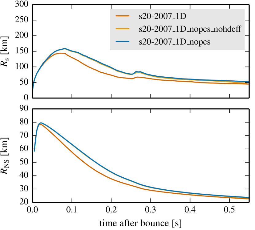
Figure 19.— Time evolution of shock radius (upper panel) and neutron star radius (lower panel) for three 1D simulations applying different neutrino physics. The neutron star radius is defined by the density surface at $10^{11}\,\mathrm{g}\,\mathrm{cm}^{-3}$. While model s20-2007_1D includes the full set of neutrino reactions, pair-conversion processes between different $\nu$ flavors and $\nu\nu$ scattering reactions are disabled in model s20-2007_1D_nopcs, and high-density nucleon correlations as well as effective mass corrections are additionally switched off in model s20-2007_1D_nopcs_nohdeff. Note that the lines for models s20-2007_1D_nopcs and s20-2007_1D_nopcs_nohdeff fall on top of each other. The curves are smoothed by running averages of 5 ms.

According to Bruenn et al. (2013, 2016), the employed neutrino physics in the Chimera and Prometheus-Vertex simulations is similar except for the treatment of in-medium nucleon correlations and nucleon-mass corrections at high densities, $\nu_{\mathrm{e}}\bar{\nu}_{\mathrm{e}}\leftrightarrow\nu_{\mu\tau}\bar{\nu}_{\mu\tau}$ pair-conversion processes, and pure neutrino-scattering reactions (Buras et al., 2003), which are not included in the Chimera code. In order to test if these differences in the neutrino physics can explain the considerable differences between the results of the Oak Ridge group (“Series B”) and the Garching group concerning shock and neutron star radii, we performed three 1D simulations of the 20 M_⊙ progenitor of Woosley & Heger (2007).

Besides a simulation with the full neutrino physics (s20-2007_1D), a second simulation was run with neutrino pair-conversion and scattering processes switched off (s20-2007_1D_nopcs) and a third simulation with high-density nucleon correlations and in-medium mass corrections (s20-2007_1D_nopcs_nohdeff) additionally disabled. The improved treatment of energy conservation described in Appendix C was also applied here. The results are shown in Fig. 19. While the omission of neutrino pair-conversion and scattering processes leads to slightly larger shock and neutron star radii, the high-density effects do not have any significant additional influence on the displayed quantities. Therefore, the differences in the applied neutrino physics cannot account for the larger shock and neutron star radii observed even in the 1D simulations with the Chimera code (Bruenn et al., 2013, 2016). Note that the neutron star radii depicted in Figure 3 of Bruenn et al. (2013) seem to be – in contrast to our previous statement – smaller than those for our models shown in Fig. 10 (second panel from top). However, since the proportionality between shock radius and neutron star radius given in Eq. (12) should also hold for the results of Bruenn et al. (2013) and the smaller neutron star radius values shown by Bruenn et al. (2013) do not make sense for their larger shock radii, we attribute this discrepancy to the accidental omission of a scaling factor in their figure.

Furthermore, a comparison to Figure 4 of Steiner et al. (2013) shows good agreement between the results of our simulations with Prometheus-Vertex and the 1D simulations with the Agile-Boltztran code, an independently developed general relativistic hydrodynamics solver with three-flavor Boltzmann neutrino transport. In view of this unsatisfactory situation further comparisons between different codes employed for CCSN simulations are indispensable in order to determine the origin of the current discrepancies in the field.

References

- Bethe & Wilson (1985) Bethe, H. A., & Wilson, J. R. 1985, ApJ, 295, 14
- Blondin et al. (2003) Blondin, J. M., Mezzacappa, A., & DeMarino, C. 2003, ApJ, 584, 971
- Bruenn et al. (2013) Bruenn, S. W., Mezzacappa, A., Hix, W. R., et al. 2013, ApJ, 767, L6
- Bruenn et al. (2016) Bruenn, S. W., Lentz, E. J., Hix, W. R., et al. 2016, ApJ, 818, 123
- Buras et al. (2003) Buras, R., Janka, H.-T., Keil, M. T., Raffelt, G. G., & Rampp, M. 2003, ApJ, 587, 320
- Buras et al. (2006a) Buras, R., Janka, H.-T., Rampp, M., & Kifonidis, K. 2006a, A&A, 457, 281
- Buras et al. (2006b) Buras, R., Rampp, M., Janka, H.-T., & Kifonidis, K. 2006b, A&A, 447, 1049
- Burrows (2012) Burrows, A. 2012, in American Institute of Physics Conference Series, Vol. 1484, American Institute of Physics Conference Series, ed. S. Kubono, T. Hayakawa, T. Kajino, H. Miyatake, T. Motobayashi, & K. Nomoto, 5–12
- Burrows & Goshy (1993) Burrows, A., & Goshy, J. 1993, ApJ, 416, L75
- Colella & Woodward (1984) Colella, P., & Woodward, P. R. 1984, Journal of Computational Physics, 54, 174
- Colgate & White (1966) Colgate, S. A., & White, R. H. 1966, ApJ, 143, 626
- Couch (2013) Couch, S. M. 2013, ApJ, 775, 35
- Couch & Ott (2013) Couch, S. M., & Ott, C. D. 2013, ApJ, 778, L7
- Couch & Ott (2015) —. 2015, ApJ, 799, 5
- Dolence et al. (2015) Dolence, J. C., Burrows, A., & Zhang, W. 2015, ApJ, 800, 10
- Ertl et al. (2016) Ertl, T., Janka, H.-T., Woosley, S. E., Sukhbold, T., & Ugliano, M. 2016, ApJ, 818, 124
- Fernández (2012) Fernández, R. 2012, ApJ, 749, 142
- Fernández et al. (2014) Fernández, R., Müller, B., Foglizzo, T., & Janka, H.-T. 2014, MNRAS, 440, 2763
- Fernández & Thompson (2009) Fernández, R., & Thompson, C. 2009, ApJ, 697, 1827
- Fischer et al. (2010) Fischer, T., Whitehouse, S. C., Mezzacappa, A., Thielemann, F., & Liebendörfer, M. 2010, A&A, 517, A80+
- Foglizzo et al. (2007) Foglizzo, T., Galletti, P., Scheck, L., & Janka, H.-T. 2007, ApJ, 654, 1006
- Foglizzo et al. (2006) Foglizzo, T., Scheck, L., & Janka, H.-T. 2006, ApJ, 652, 1436
- Fryxell et al. (1989) Fryxell, B., Müller, E., & Arnett, W. 1989, Hydrodynamics and Nuclear Burning (Garching: Max-Planck-Institut für Astrophysik)
- Gabay et al. (2015) Gabay, D., Balberg, S., & Keshet, U. 2015, ApJ, 815, 37
- Guilet & Foglizzo (2012) Guilet, J., & Foglizzo, T. 2012, MNRAS, 421, 546
- Guilet et al. (2010) Guilet, J., Sato, J., & Foglizzo, T. 2010, ApJ, 713, 1350
- Hanke (2014) Hanke, F. 2014, Dissertation, Technische Universität München, München
- Hanke et al. (2012) Hanke, F., Marek, A., Müller, B., & Janka, H.-T. 2012, ApJ, 755, 138
- Hanke et al. (2013) Hanke, F., Müller, B., Wongwathanarat, A., Marek, A., & Janka, H.-T. 2013, ApJ, 770, 66
- Hebeler et al. (2010) Hebeler, K., Lattimer, J. M., Pethick, C. J., & Schwenk, A. 2010, Physical Review Letters, 105, 161102
- Heger et al. (2005) Heger, A., Woosley, S. E., & Spruit, H. C. 2005, ApJ, 626, 350
- Janka (2001) Janka, H.-T. 2001, A&A, 368, 527
- Janka (2012) —. 2012, Annual Review of Nuclear and Particle Science, 62, 407
- Janka et al. (2012) Janka, H.-T., Hanke, F., Hüdepohl, L., et al. 2012, Progress of Theoretical and Experimental Physics, 2012, 01A309
- Janka et al. (2001) Janka, H.-T., Kifonidis, K., & Rampp, M. 2001, in Lecture Notes in Physics, Berlin Springer Verlag, Vol. 578, Physics of Neutron Star Interiors, ed. D. Blaschke, N. K. Glendenning, & A. Sedrakian, 363
- Janka et al. (2016) Janka, H.-T., Melson, T., & Summa, A. 2016, arXiv:1602.05576
- Janka et al. (2008) Janka, H.-T., Müller, B., Kitaura, F. S., & Buras, R. 2008, A&A, 485, 199
- Janka & Müller (1996) Janka, H.-T., & Müller, E. 1996, A&A, 306, 167
- Kitaura et al. (2006) Kitaura, F. S., Janka, H.-T., & Hillebrandt, W. 2006, A&A, 450, 345
- Kraichnan (1967) Kraichnan, R. H. 1967, Physics of Fluids, 10, 1417
- Kuroda et al. (2012) Kuroda, T., Kotake, K., & Takiwaki, T. 2012, ApJ, 755, 11
- Kuroda et al. (2016) Kuroda, T., Takiwaki, T., & Kotake, K. 2016, ApJS, 222, 20
- Lattimer & Swesty (1991) Lattimer, J. M., & Swesty, F. D. 1991, Nuclear Physics A, 535, 331
- Lentz et al. (2015) Lentz, E. J., Bruenn, S. W., Hix, W. R., et al. 2015, ApJ, 807, L31
- Marek et al. (2006) Marek, A., Dimmelmeier, H., Janka, H.-T., Müller, E., & Buras, R. 2006, A&A, 445, 273
- Marek & Janka (2009) Marek, A., & Janka, H.-T. 2009, ApJ, 694, 664
- Melson et al. (2015a) Melson, T., Janka, H.-T., Bollig, R., et al. 2015a, ApJ, 808, L42
- Melson et al. (2015b) Melson, T., Janka, H.-T., & Marek, A. 2015b, ApJ, 801, L24
- Müller (2015) Müller, B. 2015, MNRAS, 453, 287
- Müller et al. (2010) Müller, B., Janka, H., & Dimmelmeier, H. 2010, ApJS, 189, 104
- Müller & Janka (2014) Müller, B., & Janka, H.-T. 2014, ApJ, 788, 82
- Müller & Janka (2015) —. 2015, MNRAS, 448, 2141
- Müller et al. (2012a) Müller, B., Janka, H.-T., & Heger, A. 2012a, ApJ, 761, 72
- Müller et al. (2012b) Müller, B., Janka, H.-T., & Marek, A. 2012b, ApJ, 756, 84
- Murphy & Burrows (2008) Murphy, J. W., & Burrows, A. 2008, ApJ, 688, 1159
- Murphy & Dolence (2015) Murphy, J. W., & Dolence, J. C. 2015, arXiv:1507.08314
- Murphy et al. (2013) Murphy, J. W., Dolence, J. C., & Burrows, A. 2013, ApJ, 771, 52
- Murphy & Meakin (2011) Murphy, J. W., & Meakin, C. 2011, ApJ, 742, 74
- Nakamura et al. (2015) Nakamura, K., Takiwaki, T., Kuroda, T., & Kotake, K. 2015, PASJ, psv073, arXiv:1406.2415
- Nordhaus et al. (2010) Nordhaus, J., Burrows, A., Almgren, A., & Bell, J. 2010, ApJ, 720, 694
- O’Connor & Couch (2015) O’Connor, E., & Couch, S. 2015, arXiv:1511.07443
- O’Connor & Ott (2011) O’Connor, E., & Ott, C. D. 2011, ApJ, 730, 70
- Ott et al. (2013) Ott, C. D., Abdikamalov, E., Mösta, P., et al. 2013, ApJ, 768, 115
- Pan et al. (2016) Pan, K.-C., Liebendörfer, M., Hempel, M., & Thielemann, F.-K. 2016, ApJ, 817, 72
- Pejcha & Thompson (2012) Pejcha, O., & Thompson, T. A. 2012, ApJ, 746, 106
- Radice et al. (2016) Radice, D., Ott, C. D., Abdikamalov, E., et al. 2016, ApJ, 820, 76
- Rampp & Janka (2002) Rampp, M., & Janka, H.-T. 2002, A&A, 396, 361
- Scheck et al. (2008) Scheck, L., Janka, H.-T., Foglizzo, T., & Kifonidis, K. 2008, A&A, 477, 931
- Scheck et al. (2006) Scheck, L., Kifonidis, K., Janka, H.-T., & Müller, E. 2006, A&A, 457, 963
- Skinner et al. (2015) Skinner, M. A., Burrows, A., & Dolence, J. C. 2015, arXiv:1512.00113
- Steiner et al. (2013) Steiner, A. W., Hempel, M., & Fischer, T. 2013, ApJ, 774, 17
- Steiner et al. (2010) Steiner, A. W., Lattimer, J. M., & Brown, E. F. 2010, ApJ, 722, 33
- Suwa et al. (2010) Suwa, Y., Kotake, K., Takiwaki, T., et al. 2010, PASJ, 62, L49
- Suwa et al. (2013) Suwa, Y., Takiwaki, T., Kotake, K., et al. 2013, ApJ, 764, 99
- Suwa et al. (2016) Suwa, Y., Yamada, S., Takiwaki, T., & Kotake, K. 2016, ApJ, 816, 43
- Takiwaki et al. (2012) Takiwaki, T., Kotake, K., & Suwa, Y. 2012, ApJ, 749, 98
- Takiwaki et al. (2014) —. 2014, ApJ, 786, 83
- Tamborra et al. (2014a) Tamborra, I., Hanke, F., Janka, H.-T., et al. 2014a, ApJ, 792, 96
- Tamborra et al. (2013) Tamborra, I., Hanke, F., Müller, B., Janka, H.-T., & Raffelt, G. 2013, Physical Review Letters, 111, 121104
- Tamborra et al. (2014b) Tamborra, I., Raffelt, G., Hanke, F., Janka, H.-T., & Müller, B. 2014b, Phys. Rev. D, 90, 045032
- Thompson et al. (2005) Thompson, T. A., Quataert, E., & Burrows, A. 2005, ApJ, 620, 861
- Ugliano et al. (2012) Ugliano, M., Janka, H.-T., Marek, A., & Arcones, A. 2012, ApJ, 757, 69
- Woosley & Heger (2007) Woosley, S. E., & Heger, A. 2007, Phys. Rep., 442, 269
- Woosley et al. (2002) Woosley, S. E., Heger, A., & Weaver, T. A. 2002, Reviews of Modern Physics, 74, 1015
- Yamasaki & Yamada (2005) Yamasaki, T., & Yamada, S. 2005, ApJ, 623, 1000