Nonlin. Phen. Compl. Syst. 17 (2014) 433-438
Complex Masses of Resonances in the Potential Approach

Abstract

Quarkonium resonances in the complex-mass scale are studied. Relativistic quark potential model is used to describe the quark-antiquark system. The complex-mass formula is obtained from two exact asymptotic solutions for the QCD motivated potential with the distance-dependent value of the strong coupling in QCD. The centered masses and total widths of some meson resonances are calculated. A possible origin of the “dark matter” and the “Missing Mass”is discussed.

PACS numbers

11.10.St; 12.39.Pn; 12.40.Nn; 12.40.Yx.

Keywords

meson,quark,bound state,resonance,complex mass,width.

Introduction

The concept of resonance arises from the study of oscillating systems in classical mechanics and extends its applications to physical theories like electromagnetism, optics, acoustics, and Quantum Mechanics. In QM and Quantum Field Theory resonances may appear in similar circumstances to classical physics. However, they can also be thought of as unstable particles with the particle’s complex-energy poles in the scattering amplitude. In the version of QFT, the resonances are described by the complex-mass poles of the scattering matrix.

Most particles listed in the Particle Data Group tables [1] are unstable. A thorough understanding of the physics summarized by the PDG is related to the concept of a resonance. There are great amount and variety of experimental data and the different approaches used to extract the intrinsic properties of the resonances. There is the lack of a precise definition of what is meant by mass and width of resonance. There are two well-known definitions of mass and width of a given resonance, both widely used in the hadron physics [2]. One definition, known as the conventional approach is based on the behavior of the phase shift $\delta$ of the resonance as a function of the energy, while the other, known as the pole approach, is based on the pole position of the resonance and includes several approaches [3].

In this work, in contrast to the usual analysis of the scattering amplitude, we consider meson resonances in bound state region, i. e., quasi-bound states of the meson constituents. In traditional approach to investigate resonances one deals with the scattering theory, exploring the properties of S-matrix and partial amplitudes. In contrast to the usual analysis, meson resonances are considered to be the transient oscillations of the quark-antiquark system. We consider the bound-state problem using the potential approach and analyze the mass spectrum generated from solution of the relativistic quasi-classical (QC) wave equation.

1 The complex-mass scale

The complex numbers generalize the real numbers. These numbers are important even if one wants to find real solutions of a problem. Using complex numbers, we are getting more than what we insert. Remind the important properties of complex numbers such as the fundamental theorem of algebra, i. e., the existence of $n$ roots of any $n$-th order polynomial with complex coefficients. As known, it would’t work if we demanded real solutions. Holomorphic (natural) functions of a complex variable have many important mathematical properties that turn complex numbers into useful if not essential tools, e. g. in the case of two-dimensional conformal field theories (CFT). In many of the applications, the complex numbers may be viewed as non-essential but very useful technical tricks.

Operators in QM are Hermitian and the corresponding eigenvalues are real. However, in scattering experiment, the wave function requires different boundary condition, that is why the complex energy is required [4, 5]. There is the connection between the widths of resonances, $\Gamma_{n}$, and the imaginary part of the complex poles of the S-matrix. The full-width half-maximum of the $n$th Lorentzian peak, $\Gamma_{n}=1/\tau_{n}$, is the inverse lifetime of the resonance state, $\Gamma_{n}=1/\tau_{n}$. This analysis shows that the resonance phenomenon as obtained in a scattering experiment is mainly controlled by poles of the scattering matrix. They are associated with the scattering particle and the target which create an unstable intermediate (short-living bound) state of the system. This means we can start with the bound state problem and make the analytic continuation to the scattering region.

The concept of a purely outgoing wave belonging to the complex eigenvalue, ${\mathcal{E}}_{n}$, was introduced in 1939 by Siegert [6] that is an appropriate tool in the studying of resonances. The resonance poles are complex eigenvalues of the Hamiltonian,

$$\hat{\mathcal{H}}(r)\Psi_{n}^{res}(r)=\mathcal{E}_{n}\Psi_{n}^{res}(r),\quad\mathcal{E}_{n}=M_{n}-i\frac{\Gamma_{n}}{2},$$ (1)

where $\mathcal{E}_{n}$ is the resonance position above the threshold. Equation (1) is the basic equation in the resonance theory for time-independent Hamiltonians. The resonances in scattering experiments are associated with complex eigenvalues of the (unscaled) Hamiltonian which describes the physical system. Here $\Gamma_{n}$ corresponds to the inverse of resonance’s lifetime, $\Gamma_{n}=1/\tau_{n}$, of the resonance state.

Resonances in QFT are described by the complex-mass poles of the scattering matrix [5]. The complex eigenvalue also corresponds to a first-order pole of the S-matrix [7]. The masses of the states develop imaginary masses from loop corrections [8, 9]. In this case, the probability density comes from the particle’s propagator with the complex mass.

Resonances in hadron physics are complex values and can be described by the complex numbers. Resonance is present as transient oscillation associated with metastable states. In the pole approach the parameters $M_{p}$ and $\Gamma_{p}$ of the resonance are defined in terms of the pole position, $s_{p}$, in the complex Mandelshtam’s $s$-plane as [2, 3, 10, 11]

$$s_{p}=M_{p}^{2}-iM_{p}\Gamma_{p}.$$ (2)

Fundamentals of scattering theory and strict mathematical definition of resonances in QM was considered in [10, 11]. The rigorous QM definition of a resonance requires determining the pole position in the second Riemann sheet of the analytically continued partial-wave scattering amplitude in the complex Mandelstam $s$ variable plane [12]. This definition has the advantage of being quite universal regarding the pole position, but can only be applied if the amplitude can be analytically continued in a reliable way. It is easy to see that (2) is the approximation of the complex expression

$$\mathcal{M}_{N}^{2}=\left(M_{N}-i\frac{\Gamma_{N}}{2}\right)^{2},$$ (3)

which turns in (2) when $\Gamma_{N}\ll M_{N}$, that is usually observed in practice. The poles given by (3) are located in the fourth quadrant of the complex surface $s=\mathcal{M}^{2}$. The complex mass eigenvalues (eigenmasses), $\mathcal{M}_{N}$, can be found in the framework of the quark potential model from solution of the QC wave equation for the QCD-motivated potential.

2 The Cornell potential

The Cornell potential is a special in hadron physics. It is fixed in an extremely simple manner in terms of very small number of parameters. This potential is unique in that sense, if considered in the complex-mass scheme, it yields the complex eigenmasses for hadrons and resonances.

It is known that in perturbative QCD, as in QED the essential interaction at small distances is instantaneous Coulomb one-gluon exchange (OGE); in QCD, it is $qq$, $qg$, or $gg$ Coulomb scattering [13]. Therefore, one expects from OGE a Coulomb-like contribution to the potential, i. e., $V_{S}(r)\propto-\alpha_{s}/r$ at $r\rightarrow 0$. For large distances, in order to be able to describe confinement, the potential has to rise to infinity. From lattice-gauge-theory computations [14] follows that this rise is an approximately linear, i. e., $V_{L}(r)\simeq\sigma r+$const for large $r$, where $\sigma\simeq 0.15$ GeV² is the string tension. These two contributions by simple summation lead to the famous Cornell $q\bar{q}$ potential [14, 15],

$$V(r)=V_{S}(r)+V_{L}(r)\equiv-\frac{4}{3}\frac{\alpha_{s}}{r}+\sigma r;$$ (4)

its parameters are directly related to basic physical quantities noted above. The potential (4) is one of the most popular in hadron physics; it incorporates in clear form the basic features of the strong interaction. All phenomenologically acceptable QCD-inspired potentials are only variations around this potential.

In hadron physics, the nature of the potential is very important. There are normalizable solutions for scalar like potentials, but not for vector like. The effective interaction has to be Lorentz-scalar in order to confine quarks and gluons [16, 17]. In our consideration, we take the potential (4) to be Lorentz-scalar.

3 Two asymptotic solutions

Our aim is to find the analytic form for the resonances’ eigenmasses. This problem is not easy if one uses known relativistic wave equations with the potential (4). However, it can be done from solution of the QC wave equation for this potential [18, 19]. An important feature of this equation is that, for two and more turning-point problems, it can be solved exactly by the conventional WKB method [18, 19]. We use the advantage of analyzing the system in the complex-mass scale that has important features such as a simpler and more general framework [8, 9].

To show that, analyze the eigenvalues obtained separately for the two components of the potential (4), i. e., the Coulomb term $V_{S}(r)$ and the linear one $V_{L}(r)$. Then, using the two-point Padé approximant, we join these two exact asymptotic solutions; this results in the interpolating mass formula [20, 21]:

$$M_{N}^{2}=4\left[2\sigma\tilde{N}-\left(\frac{\tilde{\alpha}m}{N}\right)^{2}+m^{2}-2\tilde{\alpha}\sigma\right],$$ (5)

where $\tilde{\alpha}=4\alpha_{S}/3$, $\tilde{N}=N+n_{r}+1/2$, $N=n_{r}+J+1$ and $m$ is the constituent quark mass. The simple mass formula (5) describes equally well the mass spectra of all $q\bar{q}$ and $Q\bar{Q}$ quarkonia ranging from the $u\bar{d}$ ($d\bar{d}$, $u\bar{u}$, $s\bar{s}$) states up to the heaviest known $Q\bar{Q}$ systems [20, 21]. The universal formula (5) has been used to calculate the glueball masses and Regge trajectories including the Pomeron [22, 23]. It appears to be successful in many other applications.

The “saturating” Regge trajectories obtained from (5) [20, 21] were applied with success to the photoproduction of vector mesons that provide an excellent simultaneous description of the high and low $-t$ behavior of the $\gamma\,p\rightarrow p\,\rho$, $\omega$, $\phi$ cross sections [24, 25], given an appropriate choice of the relevant coupling constants [26, 27]. It was shown that the hard-scattering mechanism is incorporated in an effective way by using the “saturated” Regge trajectories that are independent of $t$ at large $-t$ [20, 21].

The mass formula (5) is very transparent physically, as well as the potential (4) (Coulomb + linear). This formula contains in a hidden form some important information; we can get it in the following way. It is easy to see that (5) is the real part of the complex expression,

$$\mathcal{M}_{N}^{2}=4\left[\left(\sqrt{2\sigma\tilde{N}}-i\frac{\tilde{\alpha}m}{N}\right)^{2}+\left(m+i\sqrt{2\tilde{\alpha}\sigma}\right)^{2}\right]\equiv 4\left[\pi_{{}_{N}}^{2}+\mu^{2}\right].$$ (6)

This expression has the form of equation for two free relativistic particles with the complex momentum,

$$\pi_{{}_{N}}=\sqrt{2\sigma\tilde{N}}-i\frac{\tilde{\alpha}m}{N},$$ (7)

and mass,

$$\mu=m+i\mu_{{\mbox{\scriptsize I}}},\quad\mu_{{\mbox{\scriptsize I}}}=\sqrt{2\tilde{\alpha}\sigma}.$$ (8)

The complex-mass expression (6) contains additional information, but let us give some ground to our consideration.

An important hint we observe studying the hydrogen atom problem. The total energy eigenvalues for the non-relativistic Coulomb problem can be written with the use of complex quantities in the form of the kinetic energy for a free particle,

$$E_{n}=\frac{p_{n}^{2}}{2m},\quad p_{n}=\frac{i\alpha m}{n_{r}+l+1}\equiv mv_{n},$$ (9)

where $p_{n}$ is the electron’s momentum eigenvalue with the imaginary discrete velocity, $v_{n}=i\alpha/(n_{r}+l+1)$. This means, that the motion of the electron in a hydrogen atom is free, but restricted by the “walls” of the potential [18, 19].

The relativistic two-body problem with the scalar-like Coulomb potential for particles of equal masses can be solved analytically [18]. The exact expression for the c. m. energy squared is written in the form of two free relativistic particles as [22, 23]:

$$E_{N}^{2}=4\left[\left(i{\rm Im}\{\pi_{{}_{N}}\}\right)^{2}+m^{2}\right],\quad{\rm Im}\{\pi_{{}_{N}}\}=\frac{\tilde{\alpha}m}{N}\equiv mv_{{}_{N}},$$ (10)

where $N$ is given above, and we have introduced the imaginary momentum eigenvalues, $i{\rm Im}\{\pi_{{}_{N}}\}$, and discrete velocity $v_{{}_{N}}$.

The linear term of the Cornell potential (4) can be dealt with analogously. In this case the exact solution is also well known [18, 22, 23]:

$$E_{N}^{2}=8\sigma\tilde{N},\quad\tilde{N}=N+\left(n_{r}+\frac{1}{2}\right).$$ (11)

This expression does not contain the mass term and can be written in the similar to (10) relativistic form,

$$E_{N}^{2}=4\left({\rm Re}\{\pi_{{}_{N}}\}\right)^{2},\quad{\rm Re}\{\pi_{{}_{N}}\}=\sqrt{2\sigma\tilde{N}},$$ (12)

where ${\rm Re}\{\pi_{{}_{N}}\}$ is the real momentum eigenvalue.

Thus, two asymptotic additive terms of the potential (4), $V_{S}(r)$ and $V_{L}(r)$, separately, yield the imaginary (10) and real (12) momentum eigenvalues. These terms of the potential represent two “different physics” (Coulomb OGE at small distances $r$ and the linear string tension at large $r$), therefore, two different realms of the interaction. Each of these two expressions, (10) and (12), is exact and was obtained independently, therefore, we can consider the complex sum, $\pi_{{}_{N}}={\rm Re}\{\pi_{{}_{N}}\}+i{\rm Im}\{\pi_{{}_{N}}\}$ given by (7). Here we accept the quark complex eigenmomentum, $\pi_{{}_{N}}$, that means the resonance total energy and mass should be complex as well.

It is an experimental fact that the dependence $M_{N}^{2}(J)$ is linear for light mesons [28]. However, at present, the best way to reproduce the experimental masses of particles is to rescale the entire spectrum given by (11) assuming that the masses of the mesons are expressed by the relation [16]

$$M_{N}^{2}=E_{N}^{2}-C^{2},$$ (13)

where $C$ is a constant energy (shift parameter). Relation (13) is used to shift the spectra and appears as a means to  simulate the effects of unknown structure approximately. But, if we rewrite (13) in the usual relativistic form,

$$M_{N}^{2}=4\left[\left({\rm Re}\{\pi_{{}_{N}}\}\right)^{2}+(\pm i\mu_{{\mbox{\scriptsize I}}})^{2}\right],$$ (14)

where ${\rm Re}\{\pi_{{}_{N}}\}$ is given by (12), we come to the concept of the imaginary mass, $\mu_{{\mbox{\scriptsize I}}}$. Here in (14) we have introduced the notation, $4(\pm i\mu_{{\mbox{\scriptsize I}}})^{2}=-C^{2}$. What is the mass $\mu_{{\mbox{\scriptsize I}}}$?

The required shift of the spectra naturally follows from the asymptotic solution of the QC wave equation for the potential (4) [18, 22, 23, 29]. To show that, we account for the “weak coupling effect”, i. e., together with the linear dependence in (12) we should include the contribution of the Coulomb term, $-\alpha_{S}/r$, of the potential. These kind of calculations result in the asymptotic expression similar to (13) [18, 22]. Comparing (15) with (14), we come to the equation:

$$M_{N}^{2}=8\sigma(\tilde{N}-\tilde{\alpha})\equiv 4\left[2\sigma\tilde{N}+(i\mu_{{\mbox{\scriptsize I}}})^{2}\right],$$ (15)

where $\mu_{{\mbox{\scriptsize I}}}$ is the quark imaginary-part mass. We see that the additional term, $-8\tilde{\alpha}\sigma$ arises from the interference of the Coulomb and linear components of the Cornell potential (4). Therefore, we have the quark real-part (constituent) mass, $\mu_{\mbox{\scriptsize R}}=m$, and the imaginary-part mass (8). As in case of the eigenmomenta, we introduce the quark complex mass, $\mu=\mu_{\mbox{\scriptsize R}}+i\mu_{{\mbox{\scriptsize I}}}$ given by (8).

The interference term $-8\tilde{\alpha}\sigma=4(i\mu_{{\mbox{\scriptsize I}}})^{2}$ in (15) contains only the parameters of the potential (4) and is Lorentz-scalar, i. e., additive to the particle masses. This is why, we accept the last additive term in (15) to be the mass term, which contributes to the quark complex mass (8). This term is negative and effectively this reduces the quark effective mass (8). This means, that a part of the quark mass goes into the interaction’s field that causes the quark’s mass defect, which is similar to one we observe in nucleus (nuclear energy).

4 The resonance’s mass and total width

Fundamentals of scattering theory and strict mathematical definition of resonances in QM was considered in [10]. It is possible to extend the Hamiltonian that describes a quantum system into the complex domain while still retaining the fundamental properties of a quantum theory. One of such approaches is Complex Quantum Mechanics (CQM) [30]. The CQM has proved to be so interesting that research activity in this area has motivated studies of complex classical mechanics [31]. Complex energies and masses cannot be measured experimentally nor simulated by lattice QCD calculations, and basically an extrapolation is needed, which is a potentially uncontrolled arbitrary procedure.

The complex eigenvalues correspond to a first-order poles of the S-matrix [7]. In order to deduce these poles reliably, one must either have narrow resonances, small backgrounds, or accurate amplitudes, requirements which are rarely met in the PDG compilation [1]. Each unstable particle in CQM is associated with a well-defined object, which is a discrete generalized eigenstate of the Hamiltonian having its real and negative imaginary parts being the centered mass, $M_{N}$, and half-width, $\Gamma_{n}/2$, of the particle, respectively [30, 31].

We have obtained two exact asymptotic solutions, i. e., (10) and (15). The complex mass (6) can be written in the form (2),

$$\mathcal{M}_{N}^{2}={\rm Re}\{\mathcal{M}_{N}^{2}\}+i{\rm Im}\{\mathcal{M}_{N}^{2}\},$$ (16)

where ${\rm Re}\{\mathcal{M}_{N}^{2}\}$ is given by the interpolating mass formula (5) [20, 21, 22, 23], and the imaginary part is given by expression:

$${\rm Im}\{\mathcal{M}_{N}^{2}\}=8m\sqrt{2\tilde{\alpha}\sigma}\left(1-\frac{\sqrt{\tilde{\alpha}\tilde{N}}}{N}\right).$$ (17)

Comparing (16) and (2), we obtain the centered mass squared, $M_{N}^{2}$, given by (5), and the total width,

$$\Gamma_{N}^{\mbox{\scriptsize TOT}}=\sqrt{2\tilde{\alpha}\sigma}\frac{8m}{M_{N}}\left|1-\frac{\sqrt{\tilde{\alpha}\tilde{N}}}{N}\right|.$$ (18)

One can consider another resonance’s definition in the pole approach. In general (mathematically), the S-matrix is a meromorphic function of complex variable $\mathcal{M}=\pm\sqrt{s}$, where the complex $s$-plane is replaced by the two-sheet Riemann surface, $\pm\sqrt{s}$, made up of two sheets $R_{0}$ and $R_{1}$, each cut along the positive real axis, Re$\mathcal{M}$, and with $R_{1}$ placed in front of $R_{0}$ [10, 12].

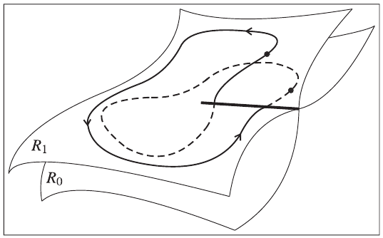
Figure 1: The two-sheet Riemann surface $\mathcal{M}=\pm\sqrt{s}$. The lower edge of the slit in $R_{0}$ is joined to the upper edge of the slit in $R_{1}$, and the lower edge of the slit in $R_{1}$ is joined to the upper edge of the slit in $R_{0}$.

The resonance positions are symmetrically located in the Riemann $\mathcal{M}$-surface (Fig. 1).

The square root of the complex expression (16) gives

$$\sqrt{\mathcal{M}_{N}^{2}}=\pm\Bigl{(}{\rm Re}\{\mathcal{M}_{N}\}+i\xi{\rm Im}\{\mathcal{M}_{N}\}\Bigr{)},$$ (19)

where

$${\rm Re}\{\mathcal{M}_{N}\}=\sqrt{\frac{|\mathcal{M}_{N}^{2}|+{\rm Re}\{\mathcal{M}_{N}^{2}\}}{2}},$$ (20)

$${\rm Im}\{\mathcal{M}_{N}\}=\sqrt{\frac{|\mathcal{M}_{N}^{2}|-{\rm Re}\{\mathcal{M}_{N}^{2}\}}{2}}=-\frac{\Gamma_{N}^{\mbox{\scriptsize TOT}}}{2},$$ (21)

$|\mathcal{M}_{N}^{2}|=\Bigl{[}\Bigl{(}{\rm Re}\{\mathcal{M}_{N}^{2}\}\Bigr{)}^{2}+\Bigl{(}{\rm Im}\{\mathcal{M}_{N}^{2}\}\Bigr{)}^{2}\Bigr{]}^{1/2}$, $\xi={\rm sgn}({\rm Im}\{\mathcal{M}_{N}^{2}\})$. The expressions (20) and (21) define the resonance position in the Riemann $\mathcal{M}$-surface. The centered mass, $M_{N}^{R}={\rm Re}\{\mathcal{M}_{N}\}$, and the total width, $\Gamma_{N}^{\mbox{\scriptsize TOT}}=-2{\rm Im}\{\mathcal{M}_{N}\}$, are process independent parameters of the resonance.

Resonance masses arise in complex conjugate pairs. Poles in the left half-plane correspond to either bound or anti-bound states [4, 32]. If $\mathcal{M}_{N}=M_{N}-i\Gamma_{N}/2$ is a pole in the fourth quadrant of the surface $\pm\sqrt{s}$, then $\mathcal{M}_{N}=-M_{N}-i\Gamma_{N}/2$ is also a pole, but in the third quadrant (antiparticle) [4]. Comprehensive definitions of the resonance’s parameters, i. e., their masses and widths, require further investigations. An alternate definition of the resonance’s width can be obtained from (17). According to the definition (2) the width is given by the imaginary-part mass of the resonance’s complex mass, $\mathcal{M}_{N}$. Dividing (17) by $8m$ (exclusion of the real-mass term), we come to the following expression:

$$\Gamma_{N}^{\mbox{\scriptsize TOT}}=\sqrt{2\tilde{\alpha}\sigma}\left|1-\frac{\sqrt{\tilde{\alpha}\tilde{N}}}{N}\right|.$$ (22)

This total width is restricted by the maximum possible value $\Gamma_{N}^{\mbox{\scriptsize max}}=\mu_{{\mbox{\scriptsize I}}}\equiv\sqrt{2\tilde{\alpha}\sigma}$ for highest excitations (resonances) at $N\rightarrow\infty$.

5 Results and discussions

Quantum theory of resonances, calculating energies, width and cross sections was considered in [4] by complex scaling. This method enables one to associate the resonance phenomenon with a single square integrable eigenfunction of the complex-scaled Hamiltonian, rather than with a collection of continuum eigenstates of the unscaled Hermitian Hamiltonian.

As an example, we have considered the $\rho$-family $J=l+1$ resonances of the leading Regge trajectory, $\alpha_{\rho}(s)$. Calculation results are in Table 1, where masses and widths are in MeV.

Table 1: Masses and total widths of the $\rho$-family resonances

Meson	$\ J^{PC}$	$\ \ M_{N}^{ex}$	$\ \ M_{N}^{th}$	$\ \ \Gamma_{N}^{ex}$	$\Gamma_{N}^{th}(\ref{ImMN})$	$\Gamma_{N}^{th}(\ref{GamnV})$
$\rho\ (1S)$	$\ \ 1^{--}$	776	775	149	150	75
$a_{2}(1P)$	$\ \ 2^{++}$	1318	1323	107	108	93
$\rho_{3}(1D)$	$\ \ 3^{--}$	1689	1689	161	170	188
$a_{4}(1F)$	$\ \ 4^{++}$	1996	1985	255	194	249
$\rho_{5}(1G)$	$\ \ 5^{--}$	$-$	2234	$-$	202	294
$a_{6}(1H)$	$\ \ 6^{++}$	$-$	2462	$-$	205	328

Parameters in these calculations are found from the best fit to the available data [1]: $\alpha_{S}=1.463$, string tension $\sigma=0.134$ GeV², the quark effective mass $m=193$ MeV. The widths $\Gamma_{N}^{th}(\ref{ImMN})$ and $\Gamma_{N}^{th}(\ref{GamnV})$ are calculated with the use of the formulas (21) and (22). The maximum width $\Gamma_{N}^{\mbox{\scriptsize max}}=\mu_{{\mbox{\scriptsize I}}}=723$ MeV. More accurate calculations require taking into account the spin-spin and spin-orbit interactions to the potential (4); the spin corrections have been considered in [20].

Location of the $\rho$-family resonances in the complex $\mathcal{M}$-surface is shown in Fig. 2.

Figure 2: The complex Riemann $\mathcal{M}=\pm\sqrt{s}$-surface. Stars show location of the complex-mass resonances relating to the leading $\rho$ Regge trajectory; the imaginary-part component of the resonances gives its half-width. Other notations are shown on the figure. Calculations done with the use of the formulas (21) and (22).

It is known that complex poles of the S-matrix always arise in conjugate pairs [32, 33]. Poles in the lower half-plane are complex-conjugated with zeros in upper half-plane. Zeros above and on the real axis correspond to bound states, and resonances are located in the lower half-plane. Purely outgoing resonant states are defined by poles in the second Riemann sheet, i. e., fourth quadrant of the complex surface ${\mathcal{M}}=\pm\sqrt{s}$ [10, 12].

Note another feature of the $\rho$-family resonance data. There is a dip ($\Gamma_{N}^{\mbox{\scriptsize TOT}}=107$ MeV) for the $a_{2}(1320)$ resonance (see Fig. 2). This dip is described in our scheme and has the following explanation. In our consideration, the resonance’s pole definition is true for all resonances except the first 1S $\rho(770)$ meson state with the quantum numbers $n_{r}=0$ and $l=0$. Equations (20) and (21) define the poles’ location in the whole two-sheet Riemann surface $\mathcal{M}=\pm\sqrt{s}$. Analysis and numerical calculations using these formulas show that the imaginary-part mass, ${\rm Im}\{\mathcal{M}_{N}\}$, of the $\rho(770)$ resonance is positive, i. e., the $\rho(770)$-state is located in the first quadrant of the complex $\mathcal{M}$-surface (${\rm Re}\{\mathcal{M}_{N}\}>0$, ${\rm Im}\{\mathcal{M}_{N}\}>0$). All other states of the $\rho(770)$-family Regge trajectory are embedded in the fourth quadrant (${\rm Re}\{\mathcal{M}_{N}\}>0$, ${\rm Im}\{\mathcal{M}_{N}\}<0$).

One can give the following explanation to this phenomenon. If we define resonance to be an excited state with non-zero quantum numbers either $l$ or $n_{r}$, then $\rho(770)$ meson with $l=0$ and $n_{r}=0$ is not resonance but the bound state with parallel spins of quarks (vector particle). This is only difference between $\rho$ and $\pi$-mesons. In this case all resonances have non-zero quantum numbers ($l\neq 0$ or $n_{r}\neq 0$, or both) and located below of the real axis. If we accept this definition, then all $(n_{r}+1)l(J^{PC})=$ $1S(J^{--})$ states are mesons if they are located in the first quadrant of the complex $\mathcal{M}$-surface.

Conclusion

The complex-scaled method is the extension of theorems and principles, which were originally proved in quantum mechanics for Hermitian operators, to non-Hermitian operators and also on the development of the complex-coordinate scattering theory. The method enables the calculation of the energy positions, lifetimes and partial widths of resonance states. We have studied meson resonances to be the quasi-bound eigenstates of two quarks interacting by the Cornell potential. Using the complex analysis, we have derived the quarkonia complex-mass formula, in which the real and imaginary parts are exact expressions. This approach has allowed us to simultaneously describe in the unified way the centered masses and total widths of the $\rho$-family resonances.

The complex-mass scale has relation to some non-Hermitian Hamiltonian. In disagreement with a widely spread belief that the width $\Gamma_{N}(M_{N})$ of meson resonances linearly depends on their mass, we have found this inconsistent with an existence of non-linear Regge trajectories. We have shown, that the Regge trajectories are non-linear analytic functions of the invariant squared mass $s=\mathcal{M}^{2}$ as their widths obtained in this work, which are restricted or decreasing with the resonance mass $M_{N}$.

Resonances represent a very economical way in theoretical description of hadronic reactions at high energies. Such a task is very important nowadays since a great significance of the width of heavy resonances. Our analysis may be important for further development of the string model of hadrons and for improvement of such transport codes as the hadron string dynamics by including the finite width of heavy resonances.

The complex masses and energies are not observable directly but may have relation to the “Missing Mass” and “Dark Matter”. We have shown in this work that the energy, momentum and mass of particles and resonances are complex. Reggeons in the Regge theory (Regge trajectories $\alpha(t)$) are the complex functions of the transfered momentum $t$ (negative invariant squared mass $s$) are the imaginary-mass hypothetical objects. But they describe the real interactions. The imaginary mass may have the same possibility to exist as the real one.

The imaginary mass is contained in the magnitude of the complex mass, $|\mathcal{M}|=(\mathcal{M}_{R}^{2}+\mathcal{M}_{{\mbox{\scriptsize I}}}^{2})^{1/2}$, and give contribution to observables. Missing Mass can perhaps be measured, and mass or energy apparently vanishing from a region of space-time may be taken as an indication that something is leaving that region, perhaps along another perpendicular axis, the imaginary one. This would mean the “Missing Mass” and “Dark Matter”…

This work was done in the framework of investigations for the experiment ATLAS (LHC), code 02-0-1081-2009/2016, “Physical explorations at LHC” (JINR-ATLAS).

References

- [1] J. Beringer. Phys. Rev. D, 86:010001, 2012.
- [2] G.L. Castro A. Bernicha and J. Pestieau. Nucl. Phys. A., 597:623, 1996.
- [3] D. Morgan and M. R. Pennington. Phys. Rev. D, 48:1185, 1993.
- [4] N. Moiseyev. Phys. Rep., 302:211, 1998.
- [5] J. R. Taylor. The Quantum Theory of Nonrelativistic Collisions. Dover Publications, 2006.
- [6] A. J. F. Siegert. Phys. Rev., 56:750, 1939.
- [7] W. Heitler and N. Hu. Phys. Rev., 159:776, 1947.
- [8] T. Bauer. Complex-mass scheme and resonances in EFT. The 8th International workshop on the physics of excited nucleons: NSTAR 2011, volume 1432. AIP Conf. Proc., Reading, Massachusetts, 2011.
- [9] M. Roth A. Denner, S. Dittmaier and D. Wackeroth. Nucl. Phys. B, 560:33, 1999.
- [10] P. D. Hislop and C. Villegas-Blas. Semiclassical szego limit of resonance clasters for the hydrogen atom stark hamiltonian. [arXiv:math-ph/1104.4466v1], 2011.
- [11] R. Brummelhuis and A. Uribe. Commun. Math. Phys., 136:567, 1991.
- [12] J. Nieves and E. R. Arriola. Phys. Lett. B, 679:449, 2009.
- [13] J. D. Bjorken and E. Paschos. Phys. Rev., 185:1975, 1969.
- [14] G. S. Bali. Phys. Rep., 343:1, 2001.
- [15] H. Mahlke E. Eichten, S. Godfrey and J. L. Rosner. Rev. Mod. Phys., 80:1161, 2008.
- [16] J. Sucher. Phys. Rev. D, 51:5965, 1995.
- [17] C. Semay and R. Ceuleneer. Phys. Rev. D, 48:5965, 1993.
- [18] M. N. Sergeenko. Mod. Phys. Lett. A, 12:2859, 1997.
- [19] M. N. Sergeenko. Phys. Rev. A, 53:3798, 1996.
- [20] M. N. Sergeenko. Z. Phys. C, 64:315, 1994.
- [21] M. N. Sergeenko. Phys. At. Nucl., 56:365, 1993.
- [22] M. N. Sergeenko. Eur. Phys. J. C, 72:2128, 2012.
- [23] M. N. Sergeenko. Europhys. Lett., 89:11001, 2010.
- [24] J. M. Laget. Phys. Rev. D, 70:054023, 2004.
- [25] M. Battaglieri. (CLAS Collaboration), Phys. Rev. Lett., 90:022002, 2003.
- [26] M. Battaglieri. (CLAS Collaboration), Phys. Rev. Lett., 87:172002, 2001.
- [27] L. Morand. (CLAS Collaboration), Eur. Phys. J. A, 24:445, 2005.
- [28] P. D. B. Collins. An Introduction to Regge Theory and High-Energy Physics. England: Cambridge Univ. Press, 1977.
- [29] M. N. Sergeenko. Int. J. Mod. Phys. A, 18:1, 2003. [arXiv:quant-ph/0010084].
- [30] D. C. Brody C. M. Bender and D. W. Hook. J. Phys. A, 41:352003, 2008.
- [31] C. Dunning P. Dorey and R. Tateo. J. Phys. A: Math. Gen., 40:R205, 2007.
- [32] L. D. Landau and E. M. Lifshitz. Quantum Mechanics. Pergamon, 1965.
- [33] N. Fernández-García and O. Rosas-Ortiz. Ann. Phys., 323:1397, 2008.