Planar three-body bound states induced by a $p$-wave interatomic resonance

Abstract

We consider the bound states of a system consisting of a light particle and two heavy bosonic ones, which are restricted in their quantum mechanical motion to two space dimensions. A $p$-wave resonance in the heavy-light short-range potential establishes the interaction between the two heavy particles. Due to the large ratio of the atomic masses this planar three-body system is perfectly suited for the Born-Oppenheimer approximation which predicts a Coulomb energy spectrum with a Gaussian cut-off.

Keywords: Few-body physics, cold-atom mixture, Born-Oppenheimer approach

1 Introduction

Borromean rings are an arrangement of three rings linked in such a way that removing one would set the other two free. In nuclear physics or in cold atoms such three-body bound states are refered to as Efimov states [1]. However, they occur only when the three particles live in three space dimensions [2, 3], and the two-particle interaction has a single $s$-wave resonance [4]. In the present article we propose a new class of three-body bound states emerging in a system composed of a light particle and two heavy bosonic ones, when the particles are restricted to two space dimensions and the heavy-light short-range interaction potential has a $p$-wave resonance. In particular, we show that this situation leads to a Coulomb energy spectrum with a Gaussian cut-off determined by the large mass ratio of the particles.

1.1 Interplay between space dimension and symmetry of resonance

In the case of a three-dimensional $s$-wave resonance, the Efimov states are supported by a underlying effective potential, which decays with the square of the distance [1, 3, 5, 6] between the particles. However, a three-dimensional $p$-wave resonance leads to an effective potential, which decays [7, 8] with the cube of the distance. Consequently, in the Efimov effect the energy spectrum depends exponentially [1, 9, 10] on the quantum number $n$, whereas in the case of the $p$-wave resonance it scales with the sixth power [7], as shown in the first row of Table 1. As a result, in the case of three dimensions, the change of the symmetry of the underlying two-body resonance results in a finite number of three-body bound state induced by the $p$-wave resonance, instead of the infinite number of the Efimov states originating from the $s$-wave resonance.

We emphasize that the shape of the effective potentials and the associated energy spectra are intimately connected to the fact that the particles experience a three-dimensional space. Indeed, in the case of a two-dimensional space there is no Efimov effect [2]. The spectrum of the three-body bound states is finite and determined by the masses of particles [11] as indicated by the left lower corner of Table 1.

Table 1: Dependence of the energy $E_{n}$ for $n\gg 1$ as well as the number $N_{b}$ of three-body bound states on the dimensionality of the problem and the symmetry of the underlying two-body resonance. Here $\alpha$, $\alpha^{\prime}$, $\beta$, and $n_{*}$ are constants determined by the masses and quantum statistics of the particles, and the number of two-body resonant interactions. Moreover, $E_{1}$ and $E_{2}$ denote the binding energies of three two-dimensional identical bosons interacting via a $s$-wave resonant potential expressed in terms of the binding energy $E_{b}$ of two bosons [2]. In the case of a $p$-wave resonance we distinguish the total angular momentum $L=0$ and $L=\pm 1$ discussed in the present article and Ref. [19], respectively.

• space	symmetry of two-body resonance
  dimension	$s$-wave	$p$-wave
  3	$E_{n}\propto\exp(-\alpha n)$	$E_{n}\propto(n_{*}-n)^{6}$
  	$N_{b}$ infinite	$N_{b}$ finite
  	(Efimov effect)
  2		$L=0$	$L=\pm 1$
  	$E_{2}=-1.27|E_{b}|$	$E_{n}\propto n^{-2}\exp(-\beta n^{2})$	$E_{n}\propto\exp[-2\exp(\alpha^{\prime}n)]$
  	$E_{1}=-16.5|E_{b}|$
  	$N_{b}$ finite	$N_{b}$ infinite	$N_{b}$ infinite

In the present article we study a three-body system composed of a light atom of mass $m$ and two heavy bosonic ones of mass $M$ with a $p$-wave resonance in the heavy-light interaction, provided the three particles are moving in two space dimensions. Due to the large mass ratio the familiar Born-Oppenheimer approximation [12] allows us to determine the effective potential by a self-consistent scattering [7] of the light particle off the two heavy ones in the case of two space dimensions. The key point of our method [7] is not to solve the Schrödinger equation for the light particle, that is a differential equation, but an equivalent system of linear algebraic equations.

Mixtures with a $p$-wave resonance have already been realized with ${\rm K}$ and ${\rm Rb}$ [13], ${\rm Li}$ and ${\rm Rb}$ [14], as well as with a Rydberg electron and a neutral atom [15], corresponding to the mass ratios $m_{\rm K}/M_{\rm Rb}\approx 0.5$, $m_{\rm Li}/M_{\rm Rb}\approx 0.1$, and $m_{\rm e}/M_{\rm Rb}\approx 10^{-5}$, respectively. Hence, the latter mixtures are promising candidates to verify our predictions. Moreover, experimentally the reduction of the dimensionality can be achieved by using off-resonant light to confine ultra-cold gases in one- or two-dimensional periodic lattices [16].

In the case of the total angular momentum $L=0$, we derive an effective potential which is the product of the Efimov potential and the inverse of the logarithm, with the length scale of the logarithm determined by the parameters of the two-dimensional $p$-wave resonance. This potential gives rise to an infinite quasi-Coulomb series

$$E_{n}=-\frac{E_{0}}{n^{2}}\exp\left(-\frac{\pi^{2}}{2}\frac{\mu}{M}\,n^{2}\right)$$ (1)

of three-body bound states for large integer $n$.

As depicted by the left column of the right lower corner of Table 1 and shown on the left of Fig. 1, the familiar Coulomb series is modified by a Gaussian cut-off governed by the mass ratio $\mu/M$, where $\mu\equiv 2mM/(m+2M)$ denotes the reduced mass and $E_{0}$ is the characteristic energy determined by the short-range physics. In order to observe many states, it is necessary to have the ratio

$$\frac{E_{n+1}}{E_{n}}\cong\exp\left[-\pi^{2}\frac{\mu}{M}\left(n+\frac{1}{2}\right)\right]$$ (2)

of the neighboring energies to be of the order of unity, giving rise to the maximum number

$$n_{\rm max}\cong\frac{1}{\pi^{2}}\frac{M}{m}$$ (3)

of observable states as $M\gg m$.

A system consisting of a Rydberg electron and two neutral atoms [17, 18] with the mass relation $M\cong 10^{5}m$, shown on the right panel of Fig. 1, represents a promising candidate to verify our predictions. In this case, equation (3) predicts that we can observe about $10^{3}$ states of the quasi-Coulomb series given by equation (1).

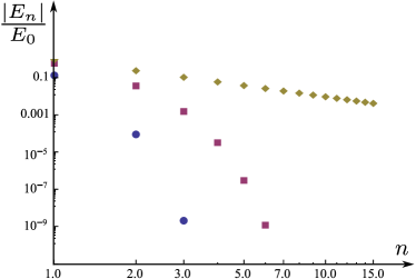
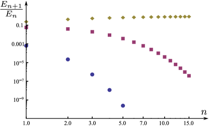
Figure 1: Quasi-Coulomb energy spectrum $E_{n}$ (left) and the resulting ratio $E_{n+1}/E_{n}$ (right) of the neighboring energy eigenvalues given by equation (1) represented in a double-logarithmic plot for three different mass ratios: $m_{\rm K}/M_{\rm Rb}=0.5$ [13] (blue dots), $m_{\rm Li}/M_{\rm Rb}=0.1$ [14] (magenta squares), $m_{\rm e}/M_{\rm Rb}=10^{-5}$ [15] (yellow diamonds).

In contrast to the case of total angular momentum $L=0$ central to the present discussion, the situation $L=\pm 1$ analyzed in Ref. [19] and summarized in the right column of the right lower corner of Table 1 leads to the “super Efimov“ effect, that is the emergence of an infinite number of the planar three-body bound states induced by the $p$-wave inter-particle resonance [20, 21].

1.2 Outline

Our article is organized as follows. In section 2 we briefly summarize the essential ingredients of our Born-Oppenheimer approach towards the three-body problem. We then employ in section 3 a scattering approach to derive a system of linear equations for the expansion coefficients of the two-dimensional waves. The effective potential for the two heavy particles follows from the condition that the determinant vanishes providing us with a transcendental equation. In section 4 we use these relations to rederive the familiar result that in the case of a planar $s$-wave resonance the Efimov effect is absent. We then dedicate section 5 to a thorough analysis of the effective potentials induced by the planar $p$-wave resonance, and discuss the resulting bound state spectrum in section 6. Finally section 7 suggests possible ways of observing the predicted bound state series. We conclude in section 8 by presenting a summary and an outlook.

In order to keep the article self-contained we include an appendix in which we establish a WKB approach towards the time-independent Schrödinger equation corresponding to the induced potentials. Here we first derive with the help of the Langer transformation [22, 23] the exact solution for zero energy, and then obtain approximate analytical expressions for non-zero energies.

2 Born-Oppenheimer approach

Since our three-body system consists of a light particle which interacts with two heavy particles, it can easily be analyzed [7, 8, 24, 25] within the Born-Oppenheimer approximation [12]. For this reason, the Schrödinger equation for the full wave function $\Phi({\bf r},{\bf R})=\Psi({\bf r};{\bf R})\chi({\bf R})$ separates into two two-dimensional equations, and the one for the light particle reads

$$\left[-\frac{\hbar^{2}}{2\mu}\Delta_{\bf r}^{(2)}+U({\bf r}_{-})+U({\bf r}_{+})\right]\Psi({\bf r};{\bf R})=-\frac{\hbar^{2}\kappa^{2}}{2\mu}\Psi({\bf r};{\bf R})$$ (4)

with ${\bf r}_{\pm}\equiv{\bf r}\pm\frac{1}{2}{\bf R}$. Here ${\bf R}$ denotes the separation between the two heavy particles and $\Delta_{\bf r}^{(2)}$ is the Laplacian in two dimensions. For the sake of simplicity we assume the potential $U$ to be cylindrically symmetric and to have the finite range $r_{0}$, that is $U(r>R_{0})=0$.

The bound-state energies

$${\mathcal{V}}({\bf R})\equiv-\frac{[\hbar\kappa({\bf R)}]^{2}}{2\mu}$$ (5)

of the light particle, corresponding to different expressions for $\kappa$ following from equation (4), serve as effective interaction potentials for the relative motion of the heavy particles given by

$$\left\{\Delta_{\bf R}^{(2)}+\frac{M}{\hbar^{2}}\left[E-{\mathcal{V}}({\bf R})\right]\right\}\chi({\bf R})=0,$$ (6)

where $E$ is the total three-body energy.

For atoms the direct heavy-heavy interaction potential is typically a short-range potential, and has for large distances a van-der-Waals tail given by $1/R^{6}$. We now show that in the case of an exact planar $p$-wave resonance, the effective potential ${\mathcal{V}}$ is a long-range one, ${\mathcal{V}}\sim 1/(R^{2}\ln R)$, and therefore the direct heavy-heavy interaction has no effect on the behavior of the total potential for large distances.

3 Interaction potential between heavy particles from scattering theory

In this section we determine ${\mathcal{V}}$ by a self-consistent scattering of the light particle off the two heavy ones in two dimensions. For this purpose, we apply the method suggested in Ref. [7] and cast equation (4) into the integral equation [12]

$$\Psi({\bf r})=\frac{\mu}{2i\hbar^{2}}\int d{\bf r}^{\prime}H_{0}^{(1)}(i\kappa|{\bf r}-{\bf r}^{\prime}|)\left[U({\bf r}_{-}^{\prime})+U({\bf r}_{+}^{\prime})\right]\Psi({\bf r}^{\prime}),$$ (7)

where $(-i/4)H_{0}^{(1)}(i\kappa|{\bf r}|)$ is the Green function of the two-dimensional Schrödinger equation (4) presented in terms of the Bessel function $H_{0}^{(1)}$ of the third kind, that is the Hankel function [26].

The Schrödinger equation (4) with a two-center potential $U({\bf r}_{-})+U({\bf r}_{+})$ is rather difficult to work with due to the fact that the solution corresponding to the two potentials is not a linear superposition of the two solutions corresponding to a single potential. However, if we regard the values of the wave function inside the potential wells as given, the wave function outside is subject to the superposition principle. Indeed, the heavy-light potential $U$ is a short-range one and the wave outside of the wells is a solution of the free Schrödinger equation in the form of a purely outgoing wave. Since the total heavy-light potential $U({\bf r}_{-})+U({\bf r}_{+})$ is nonzero only inside two spheres of radius $r_{0}$ centered at ${\bf r}=\pm\frac{1}{2}{\bf R}$, we represent equation (7) as the superposition

$$\Psi({\bf r})=\Psi^{(-)}({\bf r})+\Psi^{(+)}({\bf r})$$ (8)

of the two waves

$$\Psi^{(\pm)}({\bf r})\equiv\int\limits_{|{\bf r}^{\prime}\pm\frac{{\bf R}}{2}|\leq r_{0}}d{\bf r}^{\prime}\sigma^{(\pm)}({\bf r}^{\prime})H_{0}^{(1)}(i\kappa|{\bf r}-{\bf r^{\prime}}|)$$ (9)

with

$$\sigma^{(\pm)}({\bf r})\equiv\frac{\mu}{2i\hbar^{2}}\,U\left({\bf r}\pm\frac{1}{2}{\bf R}\right)\Psi({\bf r}).$$ (10)

The addition theorem [26]

$$H_{0}^{(1)}(i\kappa|{\bf r}-{\bf r^{\prime}}|)=\sum_{m=-\infty}^{\infty}J_{m}(i\kappa r^{\prime})H_{m}^{(1)}(i\kappa r)e^{im(\varphi_{\bf r}-\varphi_{\bf r^{\prime}})}$$ (11)

for the Bessel functions $J_{m}$ and $H_{m}^{(1)}$ with $m=0,\pm 1,\pm 2$,.. and $r>r^{\prime}$, transforms equation (9) into

$$\Psi^{(\pm)}({\bf r})=\frac{1}{\sqrt{2\pi}}\sum_{m=-\infty}^{\infty}C_{m}^{(\pm)}H_{m}^{(1)}(i\kappa r_{\pm})e^{im\varphi_{\bf r_{\pm}}},$$ (12)

with $\varphi_{\bf r}$ being the polar angle of the two-dimensional vector ${\bf r}\equiv(r\cos\varphi_{\bf r},r\sin\varphi_{\bf r})$.

We regard the coefficients $C_{m}^{(\pm)}$ determined by the integral in equation (9) as independent variables and apply scattering theory to obtain from equations (8) and (12) explicit equations for $C_{m}^{(\pm)}$ coupled by the $S$-matrix elements of the potential $U$. For this purpose, we consider a vicinity of the first potential well, that is ${\bf r}=-\frac{1}{2}{\bf R}+{\bf x}$ with $|{\bf x}|\approx r_{0}$, where the total solution

$$\Psi\left(-\frac{1}{2}{\bf R}+{\bf x}\right)=\frac{1}{\sqrt{2\pi}}\sum_{m=-\infty}^{\infty}R_{m}(|{\bf x}|)e^{im\varphi_{\bf x}}$$

given by equation (8) can be expanded into the polar harmonics $e^{im\varphi_{\bf x}}$. Here the radial wave function

$$R_{m}(|{\bf x}|)=C_{m}^{(+)}H_{m}^{(1)}(i\kappa|{\bf x}|)+J_{m}(i\kappa|{\bf x}|)\sum_{m^{\prime}=-\infty}^{\infty}H_{m-m^{\prime}}^{(1)}(i\kappa R)e^{i(m^{\prime}-m)\varphi_{\bf R}}C_{m^{\prime}}^{(-)}$$ (13)

is determined by the sum of the two contributions resulting from $\Psi^{(\pm)}(-\frac{1}{2}{\bf R}+{\bf x})$ defined by equation (12), and the sum over $m^{\prime}$ originates from the re-expansion of $H_{m}^{(1)}(i\kappa|{\bf x}-{\bf R}|)e^{im\varphi_{{\bf x}-{\bf R}}}$ into the polar harmonics $e^{im\varphi_{\bf x}}$.

In order to derive an equation for $C_{m}^{(\pm)}$ we cast the radial wave $R_{m}$ given by equation (13) into the superposition

$$R_{m}(|{\bf x}|)=a_{m}(\kappa)H_{m}^{(1)}(i\kappa|{\bf x}|)+b_{m}(\kappa)H_{m}^{(2)}(i\kappa|{\bf x}|)$$

of outgoing and incoming radial waves $H_{m}^{(1)}$ and $H_{m}^{(2)}$ with amplitudes

$$a_{m}=C_{m}^{(+)}+\frac{1}{2}\sum_{m^{\prime}=-\infty}^{\infty}H_{m-m^{\prime}}^{(1)}(i\kappa R)e^{i(m^{\prime}-m)\varphi_{\bf R}}C_{m^{\prime}}^{(-)}$$ (14)

and

$$b_{m}=\frac{1}{2}\sum_{m^{\prime}=-\infty}^{\infty}H_{m-m^{\prime}}^{(1)}(i\kappa R)e^{i(m^{\prime}-m)\varphi_{\bf R}}C_{m^{\prime}}^{(-)}.$$ (15)

Here $J_{m}$ is expressed [26] in terms of the Bessel functions of the third kind $H_{m}^{(1)}$ and $H_{m}^{(2)}$ as $J_{m}(z)=[H_{m}^{(1)}(z)+H_{m}^{(2)}(z)]/2$.

Since the amplitudes $a_{m}$ and $b_{m}$ of the outgoing and incoming waves are coupled [12, 27] by the on-shell $T$-matrix elements

$$T_{m}(i\kappa)=-\frac{1}{\pi}\frac{1}{\cot[\delta_{m}(i\kappa)]-i}$$ (16)

of the scattering potential $U$, with $\delta_{m}$ being the corresponding scattering phase, that is

$$\frac{a_{m}(\kappa)}{b_{m}(\kappa)}=1-2i\pi\,T_{m}(i\kappa),$$

we arrive at

$$C_{m}^{(+)}+i\pi\,T_{m}(i\kappa)\sum_{m^{\prime}=-\infty}^{\infty}H_{m-m^{\prime}}^{(1)}(i\kappa R)C_{m^{\prime}}^{(-)}=0.$$ (17)

Here we have used the fact that the vector ${\bf R}$ is directed along the $x$-axis, and hence $\varphi_{\bf R}=0$.

Similarly, we obtain from the second potential well centered at ${\bf r}=\frac{1}{2}{\bf R}$, the relation

$$C_{m}^{(-)}+i\pi\,T_{m}(i\kappa)\sum_{m^{\prime}=-\infty}^{\infty}H_{m^{\prime}-m}^{(1)}(i\kappa R)C_{m^{\prime}}^{(+)}=0.$$ (18)

The values of $\kappa=\kappa(R)$, and consequently the effective potential ${\mathcal{V}}$ given by equation (5), follow [7] from the condition that the determinant of the system of linear algebraic equations (17)-(18) for the coefficients $C_{m}^{(\pm)}$ vanishes. This constraint provides us with a transcendental equation for $\kappa$.

We emphasize that a similar set of equations emerges [7] in the three-dimensional case. However, the main difference in two dimensions is the appearance of the Hankel functions $H_{m}^{(1)}$ with an integer rather than a half-integer index. This substitution is a consequence of the reduced dimensionality and can be traced back to the Green function [12] of a free particle in two dimensions being proportional to $H_{0}^{(1)}$.

4 Planar $s$-wave resonance: No Efimov effect

In this section we apply our method to the case when the heavy-light interaction potential $U$ is of zero-range with a single $s$-wave resonance. This technique allows us to rederive immediately the results of Ref. [11] and serves as a guide for our next move to the uncharted territory of planar $p$-wave resonances analyzed in the following section.

The $s$-wave resonance corresponds to $m=0$ and the system of equations (17) and (18) reduces to

$$C_{0}^{(+)}+i\pi\,T_{0}(i\kappa)H_{0}^{(1)}(i\kappa R)C_{0}^{(-)}=0$$

$$C_{0}^{(-)}+i\pi\,T_{0}(i\kappa)H_{0}^{(1)}(i\kappa R)C_{0}^{(+)}=0.$$

The condition of a vanishing determinant leads us to the relation

$$i\pi\,T_{0}(i\kappa)H_{0}^{(1)}(i\kappa R)=\pm 1.$$ (19)

In the low-energy limit, that is for $\kappa r_{0}\ll 1$, the relation [28]

$$\cot[\delta_{0}(i\kappa)]\cong\frac{2}{\pi}\left[\gamma+\ln\left(\frac{i\kappa a_{0}}{2}\right)\right]$$ (20)

involves the two-dimensional scattering length $a_{0}$ linked to the energy

$$\varepsilon_{0}\equiv-2e^{-2\gamma}\frac{\hbar^{2}}{\mu a_{0}^{2}}$$ (21)

of the $s$-wave weakly-bound state in the heavy-light potential $U$ for $a_{0}\gg r_{0}$. Here $\gamma$ is the Euler constant.

When we substitute equations (16) and (20) into the condition equation (19), recall the identity $K_{m}(z)=(\pi/2)i^{m+1}H_{m}^{(1)}(iz)$ for the modified Bessel function of the second kind [26], and introduce the dimensionless variable $\xi\equiv e^{\gamma}(\kappa a_{0}/2)$, we arrive at the transcendental equation

$$K_{0}\left[\left(\frac{2}{e^{\gamma}}\frac{R}{a_{0}}\right)\xi\right]=\pm\ln\xi.$$ (22)

The two solutions $\xi_{\pm}$ of equation (22) determine the two effective potentials

$$\mathcal{V}_{\pm}(R)\equiv\varepsilon_{0}\xi_{\pm}^{2}(R),$$ (23)

shown in Fig. 2, which for large and small distances $R$ read

$${\mathcal{V}}_{+}(R)=-|\varepsilon_{0}|\left\{\begin{array}[]{ll}\frac{a_{0}}{R}\;\;\;\;\;\;\;\;\;\;\;\;\;\;\;\;\;\;\;\;\;\;\;\;\;\;\;\;\;\;\;\;\;\;\;\;\;\,{\rm for}\;R\ll a_{0}\\ \\ 1+\sqrt{\pi e^{\gamma}\frac{a_{0}}{R}}\exp\left(-\frac{2}{e^{\gamma}}\frac{R}{a_{0}}\right)\;\;{\rm for}\;R\gg a_{0}\end{array}\right.$$ (24)

and

$${\mathcal{V}}_{-}(R)=-|\varepsilon_{0}|\left\{\begin{array}[]{ll}e^{2\gamma}\ln\left(\frac{R}{a_{0}}\right)\frac{a_{0}^{2}}{R^{2}}\;\;\;\;\;\;\;\;\;\;\;\;\;\;\;\;\;\;\;\;\;{\rm for}\;R\gtrsim a_{0}\\ \\ 1-\sqrt{\pi e^{\gamma}\frac{a_{0}}{R}}\exp\left(-\frac{2}{e^{\gamma}}\frac{R}{a_{0}}\right)\;\;{\rm for}\;R\gg a_{0}.\end{array}\right.$$ (25)

As depicted in Fig. 2, the potential ${\mathcal{V}}_{-}$ is repulsive for $R\geq a_{0}$. Here we do not show ${\mathcal{V}}_{-}$ for $R<a_{0}$ since in this regime the solution $\xi_{-}$ of equation (22) is complex-valued.

In contrast to ${\mathcal{V}}_{-}$ the potential ${\mathcal{V}}_{+}$ is attractive and has the range of the order of $a_{0}$. Thus, the potential ${\mathcal{V}}_{+}$ can support only a finite number of three-body bound states, resulting in the absence [2, 11] of the Efimov effect in two dimensions.

Figure 2: Effective potentials ${\mathcal{V}}_{+}={\mathcal{V}}_{+}(R)$ (solid curve) and ${\mathcal{V}}_{-}={\mathcal{V}}_{-}(R)$ (dashed curve) induced by a $s$-wave resonant two-body interaction in two space dimensions and given by equations (22) and (23) as functions of the separation $R$ between the two heavy particles. Since ${\mathcal{V}}_{-}$ is repulsive, three-bound states can only result from the attractive potential ${\mathcal{V}}_{+}$. However, due to the exponential decay of ${\mathcal{V}}_{+}(R)$ towards $-|\varepsilon_{0}|$ for $R\rightarrow\infty$, as shown by equation (24), only a finite number of three-body bound states emerges. As a consequence, the Efimov effect does not exist in two space dimensions.

5 Planar $p$-wave resonance: Emergence of new three-body bound states

In this section we address the case of a $p$-wave resonance in the heavy-light potential $U$ and first derive the transcendental equations for $\kappa$ starting from the system of equations (17) and (18). We then solve these equations for $\kappa$ to obtain the effective potentials ${\mathcal{V}}$ given by equation (5).

5.1 Derivation of transcendental equations for $\kappa$

Similar to the expression, equation (20), for the $s$-wave scattering phase, in the low-energy limit, that is for $\kappa r_{0}\ll 1$, we can again parametrize the corresponding formula for the $p$-wave scattering phase within the two-dimensional effective-range expansion [29] by the $p$-wave effective scattering length $a_{1}$ and effective range $r_{1}$, leading us to

$$\cot[\delta_{1}(i\kappa)]\cong\frac{2}{\pi}\left[\frac{1}{a_{1}\kappa^{2}}+\ln\left(i\kappa r_{1}\right)\right].$$ (26)

Here $a_{1}$ and $r_{1}$ are non-negative parameters and for $a_{1}\gg r_{1}^{2}$ they are determined by the energy

$$\varepsilon_{1}\cong-\frac{\hbar^{2}}{\mu a_{1}\ln[a_{1}/(2r_{1}^{2})]}$$ (27)

of the $p$-wave bound state.

The latter is defined by the positive-valued pole $\kappa_{1}$ of the matrix element $T_{1}$ given by equation (16) with equation (26), that is

$$\varepsilon_{1}\equiv-\frac{\hbar^{2}\kappa_{1}^{2}}{2\mu}.$$ (28)

Moreover, in the case of a $p$-wave resonance, that is $a_{1}^{-1}=0$, the effective range $r_{1}$ has an upper bound [29] determined by the potential range $r_{0}$, that is $r_{1}\leq\frac{1}{2}e^{\gamma}r_{0}$, for any two-dimensional short-range potential.

In the case of $a_{1}^{-1}=0$ the matrix element $T_{1}$ given by equations (16) and (26) for the resonant channel is of the same order as $T_{0}$ determined by equations (16) and (20) for the non-resonant channel. Moreover, due to the scaling $T_{m>1}(i\kappa)\sim(\kappa r_{0})^{2m}$ in the low-energy limit, we need to take into account in equations (17) and (18) only the $s$- and $p$-waves, giving rise to the system

$$\begin{array}[]{r@{}l}C_{0}^{(+)}+\alpha_{1}C_{-1}^{(-)}+\alpha_{0}C_{0}^{(-)}-\alpha_{1}C_{1}^{(-)}=0\\ C_{0}^{(-)}-\alpha_{1}C_{-1}^{(+)}+\alpha_{0}C_{0}^{(+)}+\alpha_{1}C_{1}^{(+)}=0\\ C_{1}^{(+)}+\beta_{2}C_{-1}^{(-)}+\beta_{1}C_{0}^{(-)}+\beta_{0}C_{1}^{(-)}=0\\ C_{-1}^{(+)}+\beta_{0}C_{-1}^{(-)}-\beta_{1}C_{0}^{(-)}+\beta_{2}C_{1}^{(-)}=0\\ C_{1}^{(-)}+\beta_{2}C_{-1}^{(+)}-\beta_{1}C_{0}^{(+)}+\beta_{0}C_{1}^{(+)}=0\\ C_{-1}^{(-)}+\beta_{0}C_{-1}^{(+)}+\beta_{1}C_{0}^{(+)}+\beta_{2}C_{1}^{(+)}=0\end{array}$$ (29)

of six algebraic equations for $C_{0}^{(\pm)}$, $C_{1}^{(\pm)}$, and $C_{-1}^{(\pm)}$. Here we have defined the abbreviations

$$\alpha_{m}\equiv i\pi T_{0}(i\kappa)H_{m}^{(1)}(i\kappa R)$$ (30)

for $m=0,1$ and

$$\beta_{m^{\prime}}\equiv i\pi T_{1}(i\kappa)H_{m^{\prime}}^{(1)}(i\kappa R)$$ (31)

for $m^{\prime}=0,1,2$.

In order to find a non-trivial solution of equation (29), we cast equation (29) into the form of the linear equation

$${\mathcal{M}}{\bf C}=0$$ (32)

for the vector

$${\bf C}\equiv\begin{pmatrix}C_{0}^{(+)}+C_{0}^{(-)}\\ C_{1}^{(+)}-C_{-1}^{(+)}-C_{1}^{(-)}+C_{-1}^{(-)}\\ C_{0}^{(+)}-C_{0}^{(-)}\\ C_{1}^{(+)}-C_{-1}^{(+)}+C_{1}^{(-)}-C_{-1}^{(-)}\\ C_{1}^{(+)}+C_{-1}^{(+)}\\ C_{1}^{(-)}+C_{-1}^{(-)}\end{pmatrix},$$ (33)

where the matrix

$${\mathcal{M}}\equiv\begin{pmatrix}{\mathcal{M}}_{+}&0&0\\ 0&{\mathcal{M}}_{-}&0\\ 0&0&{\mathcal{M}}_{0}\end{pmatrix}$$ (34)

has the block-diagonal form, with

$${\mathcal{M}}_{\pm}\equiv\begin{pmatrix}1\pm\alpha_{0}&\pm\alpha_{1}\\ \pm 2\beta_{1}&1\pm(\beta_{2}-\beta_{0})\end{pmatrix}$$ (35)

and

$${\mathcal{M}}_{0}\equiv\begin{pmatrix}1&\beta_{0}+\beta_{2}\\ \beta_{0}+\beta_{2}&1\end{pmatrix}.$$ (36)

As a result, equation (32) has a non-trivial solution only if the determinant of ${\mathcal{M}}$ vanishes, giving rise to the two conditions

$$\beta_{0}+\beta_{2}=\mp 1,$$ (37)

and

$$(\alpha_{0}\pm 1)(\beta_{2}-\beta_{0}\pm 1)-2\alpha_{1}\beta_{1}=0.$$ (38)

When we substitute equations (16) and (26) into the condition equation (37) and recall the definition equation (31) with the identity [26] $K_{m}(z)=(\pi/2)i^{m+1}H_{m}^{(1)}(iz)$ , we arrive at the transcendental equation

$$K_{0}\left(\xi\,\frac{R}{r_{1}}\right)-K_{2}\left(\xi\,\frac{R}{r_{1}}\right)=\pm\left(\frac{r_{1}^{2}}{a_{1}}\frac{1}{\xi^{2}}+\ln\xi\right)$$ (39)

for the dimensionless variable $\xi\equiv\kappa r_{1}$.

The two solutions $\xi_{\rm I}^{(\pm)}$ of equation (39) correspond to the wave function $\Psi=\Psi({\bf r})$ of the light particle, equations (8) and (12), having the form of the symmetric, $\Psi_{{\rm I}}^{(+)}$, and asymmetric, $\Psi_{{\rm I}}^{(-)}$, superpositions of the pure $p$-waves, that is

$$\Psi_{{\rm I}}^{(\pm)}({\bf r})\propto\left[\sin(\varphi_{{\bf r}_{+}})K_{1}(\kappa r_{+})\pm\sin(\varphi_{{\bf r}_{-}})K_{1}(\kappa r_{-})\right].$$ (40)

Here the subscript ${\rm I}$ refers to the first branch.

Similarly, we can rewrite the second condition, equation (38), in the form of the transcendental equation

$$\left[K_{2}\left(\xi\frac{R}{r_{1}}\right)+K_{0}\left(\xi\frac{R}{r_{1}}\right)\pm\left(\frac{r_{1}^{2}}{a_{1}}\frac{1}{\xi^{2}}+\ln\xi\right)\right]\times$$

$$\left[K_{0}\left(\xi\frac{R}{r_{1}}\right)\mp\ln\left(\xi\frac{e^{\gamma}}{2}\frac{a_{0}}{r_{1}}\right)\right]=2K_{1}^{2}\left(\xi\frac{R}{r_{1}}\right).$$ (41)

The two solutions $\xi_{\rm II}^{(\pm)}$ of equation (41) correspond to the wave-function $\Psi=\Psi({\bf r})$ of the light particle, equations (8) and (12), having the form of the symmetric, $\Psi_{{\rm II}}^{(+)}$, and asymmetric, $\Psi_{{\rm II}}^{(-)}$, superpositions of the $s$- and $p$-waves, that is

$$\Psi_{{\rm II}}^{(\pm)}({\bf r})\propto K_{0}(\kappa r_{+})\pm K_{0}(\kappa r_{-})-A_{\pm}[\cos(\varphi_{{\bf r}_{+}})K_{1}(\kappa r_{+})\mp\cos(\varphi_{{\bf r}_{-}})K_{1}(\kappa r_{-})],$$ (42)

with $A_{\pm}\equiv[2T_{0}K_{0}(\kappa R)\pm 1][2T_{0}K_{1}(\kappa R)]^{-1}$. Here the subscript ${\rm II}$ refers to the second branch.

5.2 Solutions of two transcendental equations for $\kappa$

Next we focus on solving the two transcendental equations (39) and (41) for $\kappa$ in the case of an exact $p$-wave resonance, that is for $a_{1}^{-1}=0$, and obtaining the corresponding effective potentials ${\mathcal{V}}$, equation (5). We first address equation (39) and then turn to the slightly more complicated case of equation (41).

5.2.1 Solution of equation (39): superposition of $p$-waves

When we introduce the variable $z\equiv\xi(Rr_{1}^{-1})=\kappa R$ and use the asymptotic behavior [26] of $K_{m}(z)$ as $z\rightarrow 0$ with $m=0$ and $m=2$, we cast equation (39) for the case of $a_{1}^{-1}=0$ into the form

$$K_{0}(z)-K_{2}(z)\cong-\frac{2}{z^{2}}-\ln\frac{z}{2}-\gamma+\frac{1}{2}+\mathcal{O}\left(z^{2}\right)=\pm\left(\ln z-\ln\frac{R}{r_{1}}\right),$$ (43)

which has a solution only for the positive sign on the right-hand side as $R\gg r_{1}$ and $z\ll 1$.

Moreover, we introduce the variable $\rho\equiv\exp(\frac{1}{2}-\gamma)(Rr_{1}^{-1})$, rewrite equation (43) as

$$\frac{2}{z^{2}}=\ln\rho+\ln\frac{2}{z^{2}},$$

and solve this equation perturbativally with respect to the term $\ln(z^{2}/2)$ as $\rho\gg 1$.

As a result, we arrive at the solution

$$z^{2}\cong\frac{2}{\ln\rho+\ln\ln\rho}$$

or

$$\left(\xi_{I}^{(0)}\right)^{2}\cong\frac{2r_{1}^{2}}{R^{2}}\frac{1}{\ln\frac{R}{r_{1}}-\gamma+\frac{1}{2}+\ln\left(\ln\frac{R}{r_{1}}-\gamma+\frac{1}{2}\right)}.$$

Thus, the effective potential

$${\mathcal{V}}_{{\rm I}}^{(0)}\equiv-\frac{\hbar^{2}}{2\mu r_{1}^{2}}\left(\xi_{{\rm I}}^{(0)}\right)^{2}$$ (44)

given by equation (5) reads

$${\mathcal{V}}_{{\rm I}}^{(0)}\cong-\frac{\hbar^{2}}{\mu R^{2}}\frac{1}{\ln\frac{R}{r_{1}}-\gamma+\frac{1}{2}+\ln\left(\ln\frac{R}{r_{1}}-\gamma+\frac{1}{2}\right)}$$ (45)

for $R\gg r_{1}$.

However, near the resonance, $a_{1}\gg r_{1}^{2}$, that is in the case of the weakly-bound $p$-wave state in $U$, the effective potentials

$${\mathcal{V}}_{{\rm I}}^{(\pm)}\equiv-\frac{\hbar^{2}}{2\mu r_{1}^{2}}\left(\xi_{{\rm I}}^{(\pm)}\right)^{2}$$ (46)

are determined by the two solutions $\xi_{{\rm I}}^{(\pm)}$ of equation (39) and presented in Fig. 3. The ranges of ${\mathcal{V}}_{{\rm I}}^{(+)}$ and ${\mathcal{V}}_{{\rm I}}^{(-)}$ are identical and equal to

$$R_{1}\equiv\frac{\hbar}{\sqrt{2\mu|\varepsilon_{1}|}}\cong\left(\frac{a_{1}}{2}\ln\frac{a_{1}}{2r_{1}^{2}}\right)^{\frac{1}{2}}.$$ (47)

For large distances, $R\gtrsim R_{1}$, they approach exponentially the bound state energy $\varepsilon_{1}$ of the light particle defined by equation (27), as depicted in Fig. 3. For short distances, $R\lesssim R_{1}$, the potential ${\mathcal{V}}_{\rm I}^{(+)}$ decreases monotonically and approaches ${\mathcal{V}}_{\rm I}^{(0)}$, equation (45), whereas ${\mathcal{V}}_{\rm I}^{(-)}$ increases monotonically and vanishes at $R=\sqrt{2a_{1}}$.

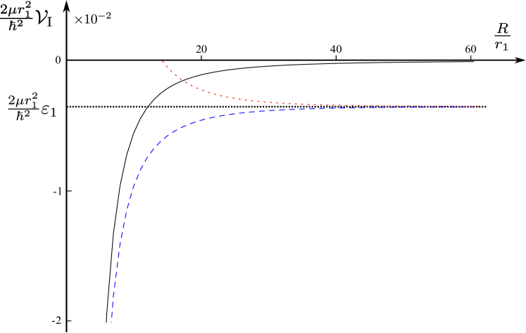
Figure 3: Effective potentials ${\mathcal{V}}_{\rm I}^{(0)}={\mathcal{V}}_{\rm I}^{(0)}(R)$ (solid black curve), ${\mathcal{V}}_{\rm I}^{(+)}={\mathcal{V}}_{\rm I}^{(+)}(R)$ (dashed blue curve), and ${\mathcal{V}}_{\rm I}^{(-)}={\mathcal{V}}_{\rm I}^{(-)}(R)$ (dotted red curve) induced by a $p$-wave resonant two-body interaction in two space dimensions and corresponding to the first branch, equations (44) and (46), as functions of the separation $R$ between the two heavy particles. Here $\varepsilon_{1}$ is the energy of the $p$-wave bound state given by equations (27) and (28) for the $p$-wave scattering length $a_{1}=100\,r_{1}^{2}$, with $r_{1}$ being the $p$-wave effective range. In complete accordance with the case of a $s$-wave resonant interaction, discussed in Fig. 2, we again find two potentials ${\mathcal{V}}_{\rm I}^{(\pm)}$, one attractive and one repulsive. However, in contrast to a $s$-wave resonance we can now have $\varepsilon_{1}=0$ corresponding to an exact $p$-wave resonance giving rise to ${\mathcal{V}}_{\rm I}^{(0)}$. Only this potential decreases appropriately for $R\rightarrow\infty$ as to support infinitely many three-body bound states.

5.2.2 Solution of equation (41): superposition of $s$- and $p$-waves

Finally we turn to the second branch of solutions of the truncated system of equations (29) determined by the transcendental equation (41).

In the case of $a_{1}^{-1}=0$, we introduce again the variable $z\equiv\xi(Rr_{1}^{-1})=\kappa R$ and use the asymptotic behavior [26] of $K_{m}(z)$ as $z\rightarrow 0$ with $m=0,1,2$, which leads us to the form

$$\left[\ln\frac{R}{r_{1}}\mp a_{\pm}\right]\left[\ln\frac{R}{r_{1}}\pm b_{\pm}\right]=-\frac{2}{z^{2}}-\ln\frac{z^{2}}{4}-2\gamma+1+\mathcal{O}(z^{2})$$ (48)

of equation (41) with the asymptotic expressions for the functions

$$a_{+}\cong\frac{2}{z^{2}}-\gamma-\frac{1}{2}+\ln 2+\mathcal{O}(z^{2})$$

$$a_{-}\cong\frac{2}{z^{2}}-\ln\frac{z^{2}}{2}-\gamma-\frac{1}{2}+\mathcal{O}(z^{2})$$

$$b_{+}\cong-2\gamma-\ln\frac{a_{0}}{r_{1}}-\ln\frac{z^{2}}{4}-\frac{z^{2}}{4}\left(\ln\frac{z}{2}+\gamma-1\right)+\mathcal{O}(z^{2})$$

$$b_{-}\cong\ln\frac{a_{0}}{r_{1}}-\frac{z^{2}}{4}\left(\ln\frac{z}{2}+\gamma-1\right)+\mathcal{O}(z^{2})$$

as $z$ tends to zero.

A solution of equation (48) occurs only with non-vanishing values of $a_{+}$ and $b_{+}$. In order to find this solution we rewrite this equation as

$$\ln\frac{R}{r_{1}}=\frac{2}{z^{2}}-\gamma-\frac{1}{2}+\ln 2-\frac{2+\mathcal{O}(z^{2})}{z^{2}\left(\ln\frac{R}{r_{1}}\right)+\mathcal{O}(z^{2})}$$

and solve it perturbativally with respect to the last term on the right-hand side, resulting in

$$\ln\frac{R}{r_{1}}\cong\frac{2}{z^{2}}-\gamma-\frac{3}{2}+\ln 2+\mathcal{O}(z^{2})$$

or

$$\left(\xi_{II}^{(0)}\right)^{2}\cong\frac{2r_{1}^{2}}{R^{2}}\frac{1}{\ln\frac{R}{2r_{1}}+\gamma+\frac{3}{2}}.$$

Thus, the effective potential

$${\mathcal{V}}_{{\rm II}}^{(0)}\equiv-\frac{\hbar^{2}}{2\mu r_{1}^{2}}\left(\xi_{{\rm II}}^{(0)}\right)^{2}$$ (49)

given by equation (5) reads

$${\mathcal{V}}_{{\rm II}}^{(0)}\cong-\frac{\hbar^{2}}{\mu R^{2}}\frac{1}{\ln\frac{R}{2r_{1}}+\gamma+\frac{3}{2}}$$ (50)

for $R\gg r_{1}$.

As a result, on the $p$-wave resonance and for $R\rightarrow\infty$, both potentials ${\mathcal{V}}_{\rm I}^{(0)}$ and ${\mathcal{V}}_{\rm II}^{(0)}$ given by equations (45) and (50) approach the same behavior

$${\mathcal{V}_{\rm I}^{(0)}}(R\rightarrow\infty)\cong{\mathcal{V}_{\rm II}^{(0)}}(R\rightarrow\infty)\cong{\mathcal{V}}(R)\equiv-\frac{\hbar^{2}}{\mu R^{2}}\frac{1}{\ln\frac{R}{r_{1}}}$$ (51)

determined by the $p$-wave effective range $r_{1}$, where $r_{1}$ is of the order of the two-body range $r_{0}$.

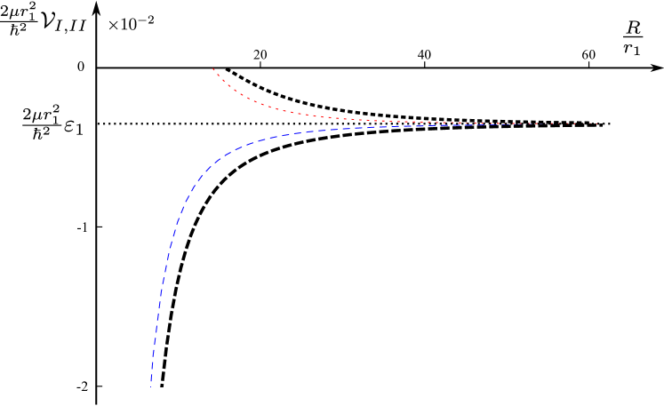
Figure 4: Effective potentials ${\mathcal{V}}_{\rm II}^{(+)}={\mathcal{V}}_{\rm II}^{(+)}(R)$ (dashed black curve) and ${\mathcal{V}}_{\rm II}^{(-)}={\mathcal{V}}_{\rm II}^{(-)}(R)$ (dotted black curve) induced by a $p$-wave resonant two-body interaction in two space dimensions and corresponding to the second branch, equation (52), compared and contrasted to the effective potentials ${\mathcal{V}}_{\rm I}^{(+)}={\mathcal{V}}_{\rm I}^{(+)}(R)$ (dashed blue curve) and ${\mathcal{V}}_{\rm I}^{(-)}={\mathcal{V}}_{\rm I}^{(-)}(R)$ (dotted red curve) of the first branch, equations (44) and (46). Here $\varepsilon_{1}$ is the energy of the $p$-wave bound state given by equations (27) and (28) for the $p$-wave scattering length $a_{1}=100\,r_{1}^{2}$ and the $s$-wave scattering length $a_{0}=10\,r_{1}$, with $r_{1}$ being the $p$-wave effective range. Whereas for short distances there is a small deviation between the potentials of different branches, asymptotically, that is for $R\rightarrow\infty$, they are identical.

In the neighborhood of the resonance, $a_{1}\gg r_{1}^{2}$, the effective potentials

$${\mathcal{V}}_{{\rm II}}^{(\pm)}\equiv-\frac{\hbar^{2}}{2\mu r_{1}^{2}}\left(\xi_{{\rm II}}^{(\pm)}\right)^{2}$$ (52)

are determined by the two solutions $\xi_{{\rm II}}^{(\pm)}$ of equation (41) and presented in Fig. 4.

6 Quasi-Coulomb energy spectrum

We are now in the position to address the two-dimensional dynamics of the two heavy bosonic particles dictated by the Schrödinger equation (6) with the potential ${\mathcal{V}}$ given by equation (51), and induced by the $p$-wave resonance in the heavy-light interaction. In particular, we show that ${\mathcal{V}}$ supports an infinite number of three-body bound states following a quasi-Coulomb series. Here we first focus our discussion on an exact resonance and then relax this requirement.

For the case of a vanishing orbital angular momentum between the two heavy bosonic particles, equation (6) describing their relative motion reduces to the radial equation

$$\left\{\frac{d^{2}}{dR^{2}}+\frac{1}{R}\frac{d}{dR}+\frac{M}{\hbar^{2}}\left[E-{\mathcal{V}}(R)\right]\right\}\chi_{E}(R)=0$$ (53)

with the WKB-solution

$$\chi_{E}(R)\cong\frac{{\mathcal{N}}_{E}}{\left\{(MR^{2}/\hbar^{2})[E-{\mathcal{V}}(R)]\right\}^{\frac{1}{4}}}\sin\left[\varphi(R,R_{E})\right]$$ (54)

derived in the Appendix. Here ${\mathcal{N}}_{E}$ is the normalization constant and the phase

$$\varphi(R,R_{E})\equiv\frac{1}{\hbar}\int_{R}^{R_{E}}dR^{\prime}\sqrt{M[E-{\mathcal{V}}(R^{\prime})]}+\theta_{E}$$ (55)

is accumulated between $R$ and the outer turning point $R_{E}$ determined by the condition ${\mathcal{V}}(R_{E})=E$. Moreover, we emphasize that the phase $\theta_{E}$ with $|\theta_{E}|\leq\pi$, which depends only weakly on the energy $E$, is determined by the behavior of the potential at short distances, that is for $R\sim r_{1}\sim r_{0}$.

6.1 Exact $p$-wave resonance

Since we are interested in the spectrum of the bound states in ${\mathcal{V}}$ close to the threshold $E=0$, we need to know the behavior of $\varphi$ as $E\rightarrow 0$. Indeed, in the limit of a slightly negative energy, $|E|\ll\hbar^{2}/(Mr_{1}^{2})$, and large distances, $r_{1}\ll R\ll R_{E}$, we show in the Appendix that we can neglect the energy $E$ under the square root on the right-hand side of equation (55) and obtain with equation (51) the approximation

$$\varphi(R,R_{E})\cong 2\sqrt{\frac{M}{\mu}}\left[\left(\ln\frac{R_{E}}{r_{1}}\right)^{\frac{1}{2}}-\left(\ln\frac{R}{r_{1}}\right)^{\frac{1}{2}}\right]+\theta_{0}$$ (56)

for the accumulated phase.

The energy spectrum of the weakly bound states caught in the potential ${\mathcal{V}}$ follows from the familiar WKB quantization rule

$$\varphi(r_{1},\rho_{n})=\pi n,$$ (57)

giving rise to the discrete positions

$$\rho_{n}\cong r_{1}\exp\left(\frac{\pi^{2}}{4}\frac{\mu}{M}\,n^{2}\right)$$ (58)

of the outer turning points for $n\gg 1$.

The connection $E_{n}={\mathcal{V}}(\rho_{n})$ between the binding energy $E_{n}$ and $\rho_{n}$ finally yields with equation (51) the asymptotic energy spectrum

$$E_{n}=-\frac{E_{0}}{n^{2}}\exp\left(-\frac{\pi^{2}}{2}\frac{\mu}{M}\,n^{2}\right)$$ (59)

for $n\gg 1$ in the form of the Coulomb series with a Gaussian cut-off governed by small mass ratio $\mu/M$. The characteristic energy $E_{0}\sim\hbar^{2}/(\mu r_{0}^{2})$ is determined by the short-range physics of the system under consideration.

Since all parameters of the short-range interaction are absorbed into the characteristic energy $E_{0}$, the spectrum given by equation (59) has a universal form and is solely determined by the mass ratio $\mu/M$ as shown in Fig. 1.

6.2 In the neighborhood of a $p$-wave resonance: number of three-body bound states

An exact two-dimensional $p$-wave resonance in the heavy-light short-range interaction potential, that is $a_{1}^{-1}=0$, creates the two long-range effective potentials ${\mathcal{V}}_{{\rm I}}^{(0)}$ and ${\mathcal{V}}_{{\rm II}}^{(0)}$ given by equations (45) and (50), respectively. They both merge into the same asymptotic potential ${\mathcal{V}}$, equation (51), which gives rise to an infinite series of the weakly bound three-body states.

However, near the resonance, that is for large but finite values of $a_{1}$, the range $R_{1}$ given by equation (47) is finite and the effective potentials ${\mathcal{V}}_{\rm I}^{(0)}$ and ${\mathcal{V}}_{\rm II}^{(0)}$ are valid only in the region $r_{1}\lesssim R\lesssim R_{1}$. As a result, the number $N_{b}$ of bound states supported by these potentials is finite and given by the number of nodes of the zero-energy solution $\chi_{0}$ defined by equation (54) with the phase $\varphi(R,R_{1})$, equation (56), accumulated between $R$ and $R_{E}\sim R_{1}$,

Since $R_{1}\gg r_{1}$, we can estimate the number

$$N_{b}\cong\frac{1}{\pi}\,\varphi(r_{1},R_{1})$$

of the three-body bound states with the help of equation (47) as

$$N_{b}\cong\frac{2}{\pi}\left(\frac{M}{\mu}\ln\frac{R_{1}}{r_{1}}\right)^{\frac{1}{2}}\cong\frac{1}{\pi}\left(2\,\frac{M}{\mu}\ln\frac{a_{1}}{2r_{1}^{2}}\right)^{\frac{1}{2}}.$$ (60)

Thus, $N_{b}$ increases with the square root of $M/\mu$ and diverges weakly as a logarithm of $a_{1}/r_{1}^{2}$ when we tune $a_{1}$ closer to the $p$-wave resonance, that is for $a_{1}\rightarrow\infty$. For this reason we obtain an infinite number of three-body bound states in the limit of an exact $p$-wave resonance.

7 Resonances in atom-molecule scattering confirm quasi-Coulomb series

We can verify experimentally the existence of the binding potentials ${\mathcal{V}}_{\rm I}^{(0)}$ and ${\mathcal{V}}_{\rm II}^{(0)}$ given by equations (45) and (50), respectively, by scattering [25, 30] a heavy atom off the diatomic molecule consisting of the heavy and the light atom. The predicted three-body bound states manifest themselves as resonances in the cross section of the atom-molecule scattering when we tune the scattering length using Feshbach resonances [31] and approach the two-dimensional $p$-wave resonance.

At the low incident energy $(\hbar k)^{2}/M\equiv E-\varepsilon_{1}$, such as $kr_{1}\ll 1$, the total atom-molecule cross-section [12]

$$\sigma_{0}=\frac{\pi^{2}}{k}\left[\frac{\pi^{2}}{4}+\ln^{2}\left(\frac{kA_{0}}{2}\,e^{\gamma}\right)\right]^{-1}$$ (61)

is determined mainly by the two-dimensional atom-molecule scattering length $A_{0}$.

In order to estimate the atom-molecule scattering length $A_{0}$ for large values of $a_{1}$ we need to solve equation (53) with $E=0$ and the potential ${\mathcal{V}}$ given by equation (51).

For the large distances $R\gtrsim R_{1}$, where the effective potential ${\mathcal{V}}$ vanishes, the zero-energy solution $\chi_{0}(R)$ of the radial Schrödinger equation (53) reads $\chi_{0}(R\gtrsim R_{1})\propto\ln(R/A_{0})$. In contrast, for the small distances $R\lesssim R_{1}$, the solution $\chi_{0}(R)$ is derived in Appendix and has the form $\chi_{0}(R\lesssim R_{1})\propto\sin[\varphi(r_{1},R)]$ with the phase $\varphi(r_{1},R)$ given by equation (56). When we match the logarithmic derivatives of these two solutions at a distance $R\sim R_{1}$, we find the relation

$$\frac{1}{\ln(R_{1}/A_{0})}=R_{1}\frac{\chi^{\prime}_{0}(R_{1})}{\chi_{0}(R_{1})}=\frac{2M}{\mu}\frac{\cot\left(\pi N_{b}\right)}{\pi N_{b}}$$

with $N_{b}$ given by equation (60).

Hence, the atom-molecule scattering length

$$A_{0}=\left(\frac{a_{1}}{2}\ln\frac{a_{1}}{2r_{1}^{2}}\right)^{\frac{1}{2}}\exp\left\{-\frac{\mu}{2M}\frac{\pi N_{b}(a_{1})}{\cot\left[\pi N_{b}(a_{1})\right]}\right\}$$ (62)

exhibits an infinite series of resonances at $a_{1}=a_{1}^{(n)}$, where $a_{1}^{(n)}$ are the zeros of the equation

$$N_{b}\left(a_{1}^{(n)}\right)=\left(n+\frac{1}{2}\right).$$ (63)

For $n\gg 1$, equation (60) provides us with the expression

$$a_{1}^{(n)}\sim r_{1}^{2}\exp\left(\frac{\pi^{2}}{2}\frac{\mu}{M}n^{2}\right)$$ (64)

for the position of the resonances in the total atom-molecule cross-section $\sigma_{0}$ given by equation (61) as a function of the two-dimensional $p$-wave scattering length $a_{1}$. For a large mass-ratio $M/\mu$ the maximum number of observable resonances is given by equation (3).

8 Summary and outlook

We have found a series of bound states in a three-body system consisting of a light particle and two heavy bosonic ones when the heavy-light short-range interaction potential has a two-dimensional $p$-wave resonance, and the system is constrained to two space dimensions. When the total angular momentum of the three particle vanishes and we tune the heavy-light interaction to an exact $p$-wave resonance, the effective potentials between the two heavy particles are attractive and of long-range. They support an infinite number of bound states and the corresponding spectrum has the form of the Coulomb series with a Gaussian cut-off governed by the mass ratio. We emphasize that these results are a consequence of an intricate interplay between the symmetry properties of the underlying resonances and the dimensionality of the problem.

We are well-aware of the fact these results are obtained within a Born-Oppenheimer approach and questions about its validity are justified. In order to answer them, we are presently developing a computer code based on parallel programming [32], which solves the Schrödinger equation for three interacting particles in two space dimensions with arbitrary masses and the heavy-light interaction being fine-tuned to the $p$-wave resonance. This approach is important from both theoretical and experimental points of view, since it will allow us to compare our approximate but analytical predictions to exact numerical solutions and those based on an adiabatic hyperspherical expansion [20, 21].

For any experiment involving mixtures of cold atoms with a large mass ratio the gravitational sag is an important issue to be reckoned with, especially in observing the quasi-Coulomb spectrum given by equation (1). Indeed, different species experience different gravitational potentials. This fact leads to a shift in the centre of the trap, and for a large mass ratio it could even result in a complete spatial separation of the individual atomic gases.

This effect can be reduced in the laboratory by a rather sophisticated arrangement of bichromatic trapping potential [33] created by overlapping optical dipole traps with two distinct wavelengths. Another very timely approach consists of bringing the experiment into a microgravity environment such as a drop tower [34], an airplane in parabolic flight [35], or a sounding rocket [36] with the International Space Station [37] being ultimate long-time low gravity platform. We are confident that such extreme conditions will lead to the experimental confirmation of the predicted quasi-Coulomb spectrum.

Appendix A Relative motion of the heavy particles: WKB approach

In this Appendix we derive the solutions of equation (53) for two different energies: (i) an exact solution for $E=0$, and (ii) an approximate solution for a slightly negative energy $E$. In the latter case we take advantage of the WKB approach [12].

A.1 Exact solution for zero energy

For this purpose we first apply the Langer transformation [22]

$$R\equiv r_{1}e^{x}$$ (65)

of the coordinate $R$ with $x\geq 0$ and cast equation (53) into the form

$$\frac{d^{2}}{dx^{2}}\,\chi+\left(\varepsilon e^{2x}+\frac{\nu_{0}}{x}\right)\chi=0.$$ (66)

Here we have introduced the dimensionless energy

$$\varepsilon\equiv\frac{Mr_{1}^{2}E}{\hbar^{2}}$$

and the effective strength

$$\nu_{0}\equiv\frac{M}{\mu}$$

of the one-dimensional Coulomb potential.

For the total three-body energy $E=0$, that is $\varepsilon=0$, equation (66) coincides with the Schrödinger equation for the one-dimensional Coulomb potential [23] $-\nu_{0}/x$ at zero energy, which with the transformation $4\nu_{0}x\equiv\zeta^{2}$ turns into

$$\left[\frac{d^{2}}{d\zeta^{2}}+\frac{1}{\zeta}\frac{d}{d\zeta}+\left(1-\frac{1}{\zeta^{2}}\right)\right]\frac{\chi_{0}}{\zeta}=0.$$ (67)

When we recall the differential equation [26]

$$\frac{d^{2}}{d\zeta^{2}}Z_{n}+\frac{1}{\zeta}\frac{d}{d\zeta}Z_{n}+\left(1-\frac{n^{2}}{\zeta^{2}}\right)Z_{n}=0$$

for the Bessel functions $Z_{n}=Z_{n}(\zeta)$, we find the analytical solution

$$\chi_{0}(x)=\sqrt{x}\left[AJ_{1}\left(2\sqrt{\nu_{0}x}\right)+BY_{1}\left(2\sqrt{\nu_{0}x}\right)\right]$$ (68)

in the form of a linear superposition of the Bessel functions $J_{1}$ and $Y_{1}$ [26] with coefficients $A$ and $B$.

Since the potential ${\mathcal{V}}$ given by equation (51) is valid only for $R\gg r_{1}$, that is $x\gg 1$, we can use the asymptotic expansion of the Bessel functions for large arguments. As a result, the exact zero-energy solution $\chi_{0}$, equation (68), reads

$$\chi_{0}(x)\propto x^{\frac{1}{4}}\sin\left(2\sqrt{\nu_{0}x}-\theta_{0}\right),$$ (69)

where the phase

$$\theta_{0}\equiv\arctan\left(\frac{B}{A}\right)+\frac{\pi}{4}$$ (70)

is determined by the potential at short distances $x\sim 1$.

A.2 Approximate solution for a slightly negative energy

Next we obtain the solution of equation (66) in the case of a slightly negative energy $\varepsilon$ by an analytical continuation of the zero-energy solution $\chi_{0}$ given by equation (68). Here we take advantage of the familiar WKB approach and find the approximate solution in the domain $1\ll x\ll x_{\varepsilon}$ governed by the outer turning point $x_{\varepsilon}$ following from the condition $x_{\varepsilon}e^{2x_{\varepsilon}}=\nu_{0}/|\varepsilon|$.

Indeed, the WKB solution

$$\chi_{\varepsilon}(x)\cong{\mathcal{N}}_{\varepsilon}\left(\frac{x}{\nu_{0}-|\varepsilon|xe^{2x}}\right)^{\frac{1}{4}}\sin\left[\varphi(x,x_{\varepsilon})\right]$$ (71)

with the quasi-classical phase

$$\varphi(x,x_{\varepsilon})\equiv\sqrt{\nu_{0}}\int_{x}^{x_{\varepsilon}}\frac{dx^{\prime}}{\sqrt{x^{\prime}}}\left(1-\frac{|\varepsilon|}{\nu_{0}}x^{\prime}e^{2x^{\prime}}\right)^{\frac{1}{2}}+\theta_{\varepsilon}$$ (72)

reproduces the exact solution $\chi_{0}$ given by equation (69) in the limit $\varepsilon\rightarrow 0$. Here ${\mathcal{N}}_{\varepsilon}$ is the normalization constant and the phase $\theta_{\varepsilon}$, which is weakly dependent on the energy $\varepsilon$ and is determined by the potential at short distances $x\sim 1$.

In order to find the energy spectrum we need to know the behavior of the phase $\varphi$ defined by equation (72) for small negative energies, $|\varepsilon|\ll 1$, and at large distances. For this purpose, we cast equation (72) into the form

$$\varphi(x,x_{\varepsilon})=\sqrt{\nu_{0}}\int_{x}^{x_{\varepsilon}}\frac{dx^{\prime}}{\sqrt{x^{\prime}}}+\theta_{\varepsilon}-\Phi$$ (73)

and show that the correction

$$\Phi\equiv\sqrt{\nu_{0}}\int_{x}^{x_{\varepsilon}}\frac{dx^{\prime}}{\sqrt{x^{\prime}}}\left[1-\left(1-\frac{|\varepsilon|}{\nu_{0}}x^{\prime}e^{2x^{\prime}}\right)^{\frac{1}{2}}\right]$$ (74)

decreases as $x_{\varepsilon}^{-\frac{1}{2}}$ as $x_{\varepsilon}\rightarrow\infty$.

Indeed, when we make in equation (74) the change of variable, $x^{\prime}\equiv x_{\varepsilon}-\xi$, we arrive at

$$\Phi=\sqrt{\frac{\nu_{0}}{x_{\varepsilon}}}\int_{0}^{x_{\varepsilon}-x}\frac{\sqrt{1-\xi/x_{\varepsilon}}}{1+\sqrt{1-(1-\xi/x_{\varepsilon})e^{-2\xi}}}\,e^{-2\xi}\,d\xi.$$ (75)

In the case of $x_{\varepsilon}\rightarrow\infty$ we can simplify the integral on the right-hand side of equation (75) to give rise to

$$\Phi\cong\sqrt{\frac{\nu_{0}}{x_{\varepsilon}}}\int_{0}^{\infty}\frac{e^{-2\xi}}{1+\sqrt{1-e^{-2\xi}}}\,d\xi=(1-\ln 2)\sqrt{\frac{\nu_{0}}{x_{\varepsilon}}},$$ (76)

where we have used the transformation $1-e^{-2\xi}\equiv z^{2}$.

Finally we use equations (65), (73), and (76) and obtain the behavior

$$\varphi(R,R_{E})\cong 2\sqrt{\frac{M}{\mu}}\left[\left(\ln\frac{R_{E}}{r_{1}}\right)^{\frac{1}{2}}-\left(\ln\frac{R}{r_{1}}\right)^{\frac{1}{2}}\right]+\theta_{E}$$ (77)

of the WKB-phase for a slightly negative energy $E$ and large distances, that is $r_{1}\ll R\ll R_{E}$.

References

References

- [1] V. Efimov, Phys. Lett. B 33, 563 (1970); Sov. J. Nucl. Phys. 12, 589 (1971); Nucl. Phys. A 210, 157 (1973)
- [2] L.W. Bruch and J.A. Tjon, Phys. Rev. A 19, 425 (1979); T.K. Lim and P.A. Maurone, Phys. Rev. B 22, 1467 (1980); S.A. Vugal’ter and G.M. Zhishin, Theor. Math. Phys. 55, 493 (1983); J. Levinsen, P. Massignan, and M.M. Parish, Phys. Rev. X 4, 031020 (2014)
- [3] A.S. Jensen, K. Riisager, D.V. Fedorov, and E. Garrido, Rev. Mod. Phys. 76, 215 (2004)
- [4] Y. Nishida, Phys. Rev. A 86, 012710 (2012)
- [5] E. Nielsen, D.V. Fedorov, A.S. Jensen, E. Garrido, Phys. Rep. 347, 373 (2001)
- [6] E. Braaten and H.-W. Hammer, Phys. Rep. 428, 259 (2006); Ann. Phys. (NY) 322, 120 (2007)
- [7] M.A. Efremov, L. Plimak, M.Yu. Ivanov, and W.P. Schleich, Phys. Rev. Lett. 111, 113201 (2013)
- [8] S. Zhu and S. Tan, Phys. Rev. A 87, 063629 (2013)
- [9] F. Ferlaino and R. Grimm, Physics 3, 9 (2010); B. Huang, L.A. Sidorenkov, R. Grimm, and J.M. Hutson, Phys. Rev. Lett. 112, 190401 (2014); S.-K. Tung, K. Jiménez-García, J. Johansen, C. Parker, and C. Chin, Phys. Rev. Lett. 113, 240402 (2014); R. Pires, J. Ulmanis, S. Häfner, M. Repp, A. Arias, E.D. Kuhnle, and M. Weidemüller, Phys. Rev. Lett. 112, 250404 (2014)
- [10] R.E. Grisenti, W. Schöllkopf, J.P. Toennies, G.C. Hegerfeldt, T. Köhler, and M. Stoll, Phys. Rev. Lett. 85, 2284 (2000); R. Brühl, A. Kalinin, O. Kornilov, J.P. Toennies, G.C. Hegerfeldt, and M. Stoll, Phys. Rev. Lett. 95, 063002 (2005); M. Kunitski, S. Zeller, J. Voigtsberger, A. Kalinin, L.Ph.H. Schmidt, M. Schöffler, A. Czasch, W. Schöllkopf, R.E. Grisenti, T. Jahnke, D. Blume, R. Dörner, Science 348, 551 (2015)
- [11] L. Pricoupenko and P. Pedri, Phys. Rev. A 82, 033625 (2010); F.F. Bellotti, T. Frederico, M.T. Yamashita, D.V. Fedorov, A.S. Jensen, and N.T. Zinner, J. Phys. B: At.Mol.Opt.Phys. 46, 055301 (2013); V. Ngampruetikorn, M.M. Parish, and J. Levinsen, EPL 102, 13001 (2013)
- [12] L.D. Landau and E.M. Lifshitz, Quantum Mechanics (Pergamon Press, Oxford, 1977)
- [13] F. Ferlaino, C. D’Errico, G. Roati, M. Zaccanti, M. Inguscio, G. Modugno, and A. Simoni, Phys. Rev. A 73, 040702(R) (2006)
- [14] B. Deh, C. Marzok, C. Zimmermann, and Ph.W. Courteille, Phys. Rev. A 77, 010701(R) (2008); C. Marzok, B. Deh, C. Zimmermann, Ph.W. Courteille, E. Tiemann, Y.V. Vanne, and A. Saenz, Phys. Rev. A 79, 012717 (2009)
- [15] I.I. Fabrikant, Journal of Physics B: Atomic and Molecular Physics 19, 1527 (1986); M. Schlagmüller, T.C. Liebisch, H. Nguyen, G. Lochead, F. Engel, F. Böttcher, K.M. Westphal, K.S. Kleinbach, R. Löw, S. Hofferberth, T. Pfau, J. Pérez-Ríos, C.H. Greene, Phys. Rev. Lett. 116, 053001 (2016)
- [16] I. Bloch, J. Dalibard, and W. Zwerger, Rev. Mod. Phys. 80, 885 (2008)
- [17] V. Bendkowsky, B. Butscher, J. Nipper, J.B. Balewski, J. P. Shaffer, R. Löw, T. Pfau, W. Li, J. Stanojevic, T. Pohl, and J.M. Rost, Phys. Rev. Lett. 105, 163201 (2010)
- [18] E.L. Hamilton, C.H. Greene, and H.R. Sadeghpour, J. Phys. B: At. Mol. Opt. Phys. 35, L199 (2002); C.H. Greene, A.S. Dickinson, and H.R. Sadeghpour, Phys. Rev. Lett. 85, 2458 (2000)
- [19] Y. Nishida, S. Moroz, and D.T. Son, Phys. Rev. Lett. 110, 235301 (2013); S. Moroz and Y. Nishida, Phys. Rev. A 90, 063631 (2014)
- [20] D.K. Gridnev, J. Phys. A: Math. Theor. 47, 505204 (2014)
- [21] A.G. Volosniev, D.V. Fedorov, A.S. Jensen, and N.T. Zinner, J. Phys. B: At. Mol. Opt. Phys. 47, 185302 (2014); C. Gao, J. Wang, and Z. Yu, Phys. Rev. A 92, 020504(R) (2015)
- [22] R.E. Langer, Phys. Rev. 51, 669 (1937); J.P. Dahl and W.P. Schleich, J. Phys. Chem. A 108, 8713 (2004)
- [23] R. Loudon, Am. J. Phys. 27, 649 (1959)
- [24] A.C. Fonseca, E.F. Redish, and P.E. Shanley, Nuclear Physics A 320, 273 (1979)
- [25] M.A. Efremov, L. Plimak, B. Berg, M.Yu. Ivanov, and W.P. Schleich, Phys. Rev. A 80, 022714 (2009)
- [26] Handbook of Mathematical Functions, edited by M. Abramowitz and I.A. Stegun (Dover, New York, 1972)
- [27] R.G. Newton, Scattering Theory of Waves and Particles (Springer, Heidelberg, 1982)
- [28] D. Bollé and F. Gesztesy, Phys. Rev. Lett. 52, 1469 (1984); B.J. Verhaar, J.P.H.W. van den Eijnde, M.A.J. Voermans, and M.M.J. Schaffrath, J. Phys. A: Math.Gen. 17, 595 (1984)
- [29] H.-W. Hammer and D. Lee, Ann. Phys. (NY) 325, 2212 (2010); M. Randeria, J.M. Duan, and L.Y. Shieh, Phys. Rev. B 41, 327 (1990); S.A. Rakityansky and N. Elander, J. Phys. A: Math.Theor. 45, 135209 (2012)
- [30] K. Helfrich, H.-W. Hammer, and D. S. Petrov, Phys. Rev. A 81, 042715 (2010)
- [31] C. Chin, R. Grimm, P. Julienne, and E. Tiesinga, Rev. Mod. Phys. 82, 1225 (2010)
- [32] We perform our numerical simulations on the recently invented high-performance computer ”Hypatia” of Data Vortex Technology (http://www.datavortex.com).
- [33] J. Ulmanis, S. Häfner, R. Pires, F. Werner, D.S. Petrov, E.D. Kuhnle, and M. Weidemüller, Phys. Rev. A 93, 022707 (2016)
- [34] T. van Zoest et al., Science 328, 1540 (2010); H. Müntinga et al. Phys. Rev. Lett. 110, 093602 (2013)
- [35] R. Geiger et al., Nat. Commun. 2, 474 (2011)
- [36] H. Ahlers et al., Phys. Rev. Lett. 116, 173601 (2016)
- [37] J. Williams, S. Chiow, N. Yu, and H. Müller, New J. Phys. 18, 18 025018 (2016)