Asymptotic behavior for the critical nonhomogeneous porous medium equation in low dimensions

Abstract

We deal with the large time behavior for a porous medium equation posed in nonhomogeneous media with singular critical density

$$|x|^{-2}\partial_{t}u(x,t)=\Delta u^{m}(x,t),\quad(x,t)\in\mathbb{R}^{N}\times(0,\infty),\ m\geq 1,$$

posed in dimensions $N=1$ and $N=2$, which are also interesting in applied models according to works by Kamin and Rosenau. We deal with the Cauchy problem with bounded and continuous initial data $u_{0}$. We show that in dimension $N=2$, the asymptotic profiles are self-similar solutions that vary depending on whether $u_{0}(0)=0$ or $u_{0}(0)=K\in(0,\infty)$. In dimension $N=1$, things are strikingly different, and we find new asymptotic profiles of an unusual mixture between self-similar and traveling wave forms. We thus complete the study performed in previous recent works for the bigger dimensions $N\geq 3$.

AMS Subject Classification 2010: 35B33, 35B40, 35K10, 35K67, 35Q79.

Keywords and phrases: porous medium equation, non-homogeneous media, singular density, asymptotic behavior, radially symmetric solutions, nonlinear diffusion.

1 Introduction

The goal of this work is to study the asymptotic behavior of solutions to the following nonhomogeneous porous medium equation with critical singular density

$$|x|^{-2}\partial_{t}u(x,t)=\Delta u^{m}(x,t),\quad(x,t)\in\mathbb{R}^{N}\times(0,\infty),$$ (1.1)

where $m\geq 1$ and we restrict ourselves to low dimensions $N=1$ and $N=2$. This completes the panorama of the large time behavior of solutions to Eq. (1.1), already studied in dimensions $N\geq 3$ in previous recent works by the authors [12, 13]. We will work with the Cauchy problem for initial data satisfying

$$u(x,0)=u_{0}(x)\in L^{\infty}(\mathbb{R}^{N})\cap C(\mathbb{R}^{N}),\ u_{0}\geq 0,\ u_{0}\not\equiv 0,\quad{\rm for\ any}\ x\in\mathbb{R}^{N}.$$ (1.2)

Moreover, unless we explicitly state the contrary, we will always consider radially symmetric initial conditions, that is, $u_{0}(x)=u_{0}(r)$, $r=|x|$.

Equations such as

$$\varrho(x)\partial_{t}u(x,t)=\Delta u^{m}(x,t),\quad(x,t)\in\mathbb{R}^{N}\times(0,\infty),$$ (1.3)

where $\varrho$ is a density function with suitable behavior, have been proposed by Kamin and Rosenau in several classical papers [15, 16, 17] as a model for thermal propagation by radiation in non-homogeneous plasma. Afterwards, a big development of the mathematical theory associated to Eq. (1.3) begun, assuming that the density satisfies

$$\varrho(x)\sim|x|^{-\gamma},\quad\hbox{as}\ |x|\to\infty,$$

for some $\gamma>0$, as for example in the following papers [6, 7, 8, 10, 24, 28, 25, 26, 14, 21] where its qualitative properties and asymptotic behavior are studied. In particular, some of these works were also considering purely singular densities such as $\varrho(x)=|x|^{-\gamma}$, and proving that asymptotic profiles for (1.3) come from explicit solutions to equations with singular density. Moreover, it came out that the density $\varrho(x)=|x|^{-2}$ (or $\varrho(x)\sim|x|^{-2}$ as $|x|\to\infty$) is critical for both the qualitative properties (well-posedness, regularity) and large time behavior: indeed, for $\gamma\in(0,2)$, properties do not depart from those already well investigated of the porous medium equation $u_{t}=\Delta u^{m}$, while for $\gamma>2$, they are different.

Restricting ourselves to the singular case $\varrho(x)=|x|^{-\gamma}$, its theory developed later, due to the difficulties involved by the presence of the singular coefficient. Some results on qualitative behavior were established in [10], then later in [14, Section 6] and [21, Section 3], the latter two using weighted spaces for well-posedness, and restricting the study to dimensions $N\geq 3$. On the other hand, formal transformations and explicit solutions were established in [8, 11], where it becomes clear why $\gamma=2$ is a critical exponent. Restricting to (1.1), the large time behavior in dimensions $N\geq 3$ has been established recently by the authors [12, 13], and the results were quite striking: the presence of both critical density $\gamma=2$ and the singularity at $x=0$ led to many new and unexpected mathematical phenomena, that in the general, non-critical and/or non-singular case do not happen. We recently learned that also the nonhomogeneous equation for the fractional porous medium

$$\varrho(x)\partial_{t}u=(-\Delta)^{s}(u^{m}),\quad m>1,\ s\in(0,1),$$

has been proposed in [9], where the qualitative properties and large time behavior are studied for suitable $\varrho(x)$, but again excluding the critical density (that in the fractional case holds for $\gamma=2s$).

1.1 Main results

We are now ready to state the main results of this paper. As already explained, we deal with radially symmetric solutions $u(x,t)$ to Eq. (1.1) having initial condition $u_{0}$ as in (1.2). We refer the reader to Section 2 for the well-posedness of the Cauchy problem (1.1)-(1.2) in our framework, and also to some changes of function and variable converting (1.1) into other nonlinear diffusion equations. As also seen in our precedent works [12, 13], an important difference in the asymptotic behavior will appear with respect to the value of $u_{0}$ at the origin: profiles are very different when $u_{0}(0)=0$ or $u_{0}(0)=K$.

But the main motivation for us to write this paper is that the large time behavior differs according to the dimension $N=1$ and $N=2$ and in some cases strikingly departs from the parallel results in dimension $N\geq 3$ given in [13]. We state in the sequel the results corresponding to $m>1$, as the case $m=1$ is easy and is reduced to a comment in Section 5.

Large time behavior in dimension $N=2$. The asymptotic profiles to Eq. (1.1) with $m>1$ and in dimension $N=2$ are of self-similar type, but with logarithmic variables. This is explained by the fact that there exists a one-to-one correspondence between radially symmetric solutions to (1.1) and solutions to the standard porous medium equation

$$\partial_{t}w(s,t)=\partial_{ss}(w^{m})(s,t),\qquad(s,t)\in\mathbb{R}\times(0,\infty),$$ (1.4)

in one dimension. We next state the precise results.

Theorem 1.1.

Let $u$ be a solution to (1.1) with $m>1$ and posed in dimension $N=2$, with radially symmetric initial condition $u_{0}$, satisfying (1.2) and moreover the following integral condition (in radial variables)

$$u_{0}(0)=0,\qquad\int_{0}^{\infty}\frac{u_{0}(r)}{r}\,dr<\infty.$$ (1.5)

Then we have

$$\lim\limits_{t\to\infty}t^{\alpha}\|u(\cdot,t)-U_{0}(\cdot,t)\|_{\infty}=0,\qquad\alpha=\frac{1}{m+1},$$ (1.6)

where

$$U_{0}(x,t)=t^{-\alpha}\left[C_{0}-k\left(\frac{\log\,|x|}{t^{\alpha}}\right)^{2}\right]_{+}^{1/(m-1)},\qquad k=\frac{m-1}{2(m+1)},$$ (1.7)

and $C_{0}=C(u_{0})$ is uniquely determined by the initial condition $u_{0}$.

In the case when $u_{0}(0)=K>0$, the asymptotic profile is non-explicit but nevertheless it still has self-similar form. More precisely

Theorem 1.2.

Let $u$ be a solution to (1.1) with $m>1$ and posed in dimension $N=2$, with radially symmetric initial condition $u_{0}$, satisfying (1.2) and moreover

$$u_{0}(0)=K>0,\qquad\lim\limits_{|x|\to\infty}u_{0}(x)=0.$$

Then there exists a radially symmetric profile

$$W(x,t)=f\left(\frac{\log\,|x|}{\sqrt{t}}\right),\qquad W(0,t)=K,\ {\rm for\ any}\ t>0,$$ (1.8)

such that

$$\lim\limits_{t\to\infty}\|u(\cdot,t)-W(\cdot,t)\|_{\infty}=0.$$ (1.9)

In particular, we also get that $u(0,t)=K$ for any $t>0$, that is, the value at the origin do not change along the evolution.

Remarks. 1. Let us notice that, while Theorem 1.1 requires some control of the tail of $u_{0}$ (via (1.5)), in Theorem 1.2 there is no need for such control, only that $u_{0}(r)\to 0$ as $r\to\infty$. This is explained by the fact that, when $u_{0}(0)=K>0$, there is no time decay rate $t^{-\alpha}$ and thus, the global large time behavior is dominated by the inner behavior, that is, in dynamic regions close to $x=0$.

2. The profile $W$ (or $f$) in (1.8) comes from a special self-similar solution to (1.4) which is not explicit, but it was introduced via a scaling process in [1, 29]. More details about it in Subsection 3.2 below, where its properties are recalled.

3. Results in Theorem 1.2 remind of those for the similar equation in dimension $N\geq 3$, see [13, Theorem 1.6], although the profile there is explicit. Meanwhile, Theorem 1.1 departs strongly from the results in dimensions $N\geq 3$, [13, Theorem 1.4], as there the profiles were coming via an asymptotic simplification to a conservation law leading to peak-form profiles, while in the present case we have a regular, self-similar type function.

Large time behavior in dimension $N=1$. In this case, things are surprisingly different, although in appearance the equation is the same. The is understood via some natural change of variable indicated at the end of Section 2, leading to a porous medium equation with convection:

$$\partial_{t}w(s,t)=\partial_{ss}(w^{m})(s,t)-\partial_{s}(w^{m})(s,t),\qquad(s,t)\in\mathbb{R}\times(0,\infty),$$ (1.10)

whose behavior (of traveling waves type) is essentially different from the one for the standard porous medium equation (1.4). There is once more a difference on whether $u_{0}(0)=0$ or $u_{0}(0)>0$.

The case of initial conditions $u_{0}$ with $u_{0}(0)=0$ is largely similar to the equivalent case in [13]. As there, we will get an asymptotic profile presenting a peak-type discontinuity, thus, the uniform convergence will be replaced by a slightly weaker concept, the convergence in the sense of graphs for multivalued functions, which allows us to deal with jump discontinuities. For the sake of completeness, we recall here this concept (following [5, 13]). Let $f$, $g:D\subseteq\mathbb{R}\mapsto 2^{\mathbb{R}}$ be two multivalued functions. We define the distance between their graphs as

$$d_{g}(f(x),g(x))=\inf\{|y-z|:y\in f(x),\ z\in g(x)\},\qquad{\rm for\ any}\ x\in D.$$

Let $\{f_{k}\}:D\subseteq\mathbb{R}\mapsto 2^{\mathbb{R}}$ be a sequence of multivalued functions and $F:D\subseteq\mathbb{R}\mapsto 2^{\mathbb{R}}$. We say that ${f_{k}}$ converges in the sense of graphs to $F$ if for any $\varepsilon>0$, there exists $k(\varepsilon)>0$ sufficiently large such that

$$d_{g}(f_{k}(x),F(x))\leq\varepsilon,\qquad{\rm for\ any}\ k\geq k(\varepsilon),\ x\in D.$$

Notice that, in the standard case of univalued functions, this notion reduces to the usual uniform convergence. In the case of a function $F$ having a jump discontinuity at $x_{0}\in D$ (as it will be our case below), letting

$$l_{-}:=\lim\limits_{x\to x_{0}^{-}}F(x)<\lim\limits_{x\to x_{0}^{+}}F(x)=l_{+},$$

we will work with $F(x_{0})=[l_{-},l_{+}]$. We define, for a measurable function $h$, the norm

$$\|h\|_{p,1}:=\left(\int_{\mathbb{R}}\frac{|h(x)|^{p}}{|x|}\,dx\right)^{1/p}.$$

With these definitions, we are now ready to state our convergence result.

Theorem 1.3.

Let $u$ be a solution to (1.1) with $m>1$, posed in dimension $N=1$, with radially symmetric initial condition $u_{0}$ satisfying (1.2) and moreover

$$u_{0}(0)=0,\qquad M_{0}:=\int_{0}^{\infty}\frac{u_{0}(x)}{x}\,dx<\infty.$$ (1.11)

Then:

(a) For any $p\in[1,\infty)$, we have

$$\lim\limits_{t\to\infty}t^{(p-1)/mp}\|u(\cdot,t)-F(\cdot,t)\|_{p,1}=0,$$ (1.12)

where

$$F(x,t)=\left\{\begin{array}[]{ll}t^{-1/m}\left[\frac{1}{m}t^{-1/m}\log\,|x|\right]_{+}^{1/(m-1)},&{\rm for}\ 0<|x|<e^{kt^{1/m}},\\ 0,&{\rm for}\ |x|\geq e^{kt^{1/m}}.\end{array}\right.$$ (1.13)

and $k=k(M_{0})$ depends only on $M_{0}$.

(b) Introducing self-similar changes of variable and function

$$\overline{u}(y,t)=t^{1/m}u(x,t),\qquad\overline{F}(y)=t^{1/m}F(y,t)=\left[\frac{y}{m}\right]^{1/(m-1)},\ y=t^{-1/m}\log\,|x|,$$ (1.14)

we have

$$\overline{u}(y,t)\longrightarrow\overline{F}(y),\qquad{\rm as}\ t\to\infty,$$ (1.15)

the convergence being in the sense of graphs.

Remarks. 1. It is obvious that we cannot get uniform convergence in (1.12) (by letting $p\to\infty$), as the limit profile $F$ presents a peak-type discontinuity and it cannot thus be a uniform limit of continuous functions. The convergence in the sense of graphs replaces the uniform convergence here.

2. The results are quite similar to [13, Theorems 1.1 and 1.4]. The main difference with respect to there is that the direction of evolution of the profile is forward, as in dimension $N\geq 3$ it evolves backward.

3. Faster decay in the inner region. The fact that the limit profile vanishes for $x\in[0,1]$ only means that in that region, the solutions decay in time faster than the global time scale $t^{-1/m}$. Indeed, we infer from the self-map (inversion) for (1.1) between dimensions $N=3$ and $N=1$ (see [11, Section 2.1]), and from the large time behavior in outer regions for $N\geq 3$ [21, Theorem 1.1] and [13, Theorem 1.11], that the large time behavior in inner regions near $x=0$ states

$$\lim\limits_{t\to\infty}t^{1/(m-1)}\|u(\cdot,t)-B_{D}(\cdot,t)\|_{\infty}=0,\qquad{\rm uniformly\ in\ sets}\ \{|x|\leq\delta t^{-1/(m-1)}\},$$

for any $\delta>0$, where $B_{D}$ is an explicit profile,

$$B_{D}(x,t)=t^{-1/(m-1)}\left[D+\frac{1}{m}\log\left(|x|t^{1/(m-1)}\right)\right]_{+}^{1/(m-1)},$$

for some $D>0$ depending only on the initial condition $u_{0}$. This shows in particular that the time decay rate in inner regions of the form above is faster, as expected ($t^{-1/(m-1)}$ instead of the global $t^{-1/m}$), whence the uniform vanishing near $x=0$ of the global profile $F$ in (1.13).

4. The appearance of a peak-type profile is a very surprising and interesting result at first sight. It is explained by the fact that Eq. (1.10) lies in a regime where the convection term dominates on the large-time evolution, producing limit profiles characteristic to conservation laws, not to diffusion equations.

When $u_{0}(0)=K>0$, the asymptotic profiles are of a ”special self-similar” type. This comes in fact from a traveling wave profile in transformed variables. More precisely,

Theorem 1.4.

Let $u$ be a solution to (1.1) with $m>1$, posed in dimension $N=1$, with radially symmetric initial condition $u_{0}$ satisfying (1.2) and moreover

$$u_{0}(0)=K>0,\qquad\lim\limits_{|x|\to\infty}u_{0}(x)=0,\qquad 0\leq u_{0}(x)\leq K,\ {\rm for\ any}\ x\in\mathbb{R},$$ (1.16)

and

$$u_{0}\in C^{0,\alpha}(\mathbb{R}),\ {\rm for\ some}\ \alpha\in(0,1].$$ (1.17)

Then, there exists $x_{0}>0$ (depending only on $u_{0}$) such that

$$\lim\limits_{t\to\infty}\|u(\cdot,t)-U_{x_{0}}(\cdot,t)\|_{\infty}=0,$$ (1.18)

where

$$U_{x_{0}}(x,t)=\left[K^{m-1}-\left(\frac{|x|}{x_{0}}e^{-ct}\right)^{(m-1)/m}\right]_{+}^{1/(m-1)},\qquad c=K^{m-1}.$$ (1.19)

The dependence of $x_{0}$ on the initial condition $u_{0}$ is given via an integral condition in transformed variables, see (4.5) in Subsection 4.2.

Remarks. 1. Profiles (1.19) were first obtained in [8, Section 7]. The form of them is not standard self-similar.

2. In fact, we have a family of profiles $U_{x_{0}}$, for any $x_{0}\in\mathbb{R}$, and one can readily notice that they are not equivalent, that is,

$$\|U_{x_{0}}(\cdot,t)-U_{y_{0}}(\cdot,t)\|\not\to 0,\qquad{\rm as}\ t\to\infty,$$

for $x_{0}\neq y_{0}$. Thus, it is a relevant fact that we can identify the exact translation parameter $x_{0}$, only in terms of the initial condition $u_{0}$.

3. Result for non-radial solutions. In dimension $N=1$, we are able to extend the large time behavior to solutions with general (not radially symmetric) data $u_{0}$. We postpone this fact to the final section, see (5.7) for a result.

Organization of the paper. We begin with a rather standard section which gathers well-posedness and some preliminary facts about the solutions to (1.1), that are later used in the proofs. We devote further Sections 3 and 4 to the proofs of the main results Theorems 1.1 and 1.2 (concerning dimension $N=2$), respectively Theorems 1.3 and 1.4 (concerning dimension $N=1$). Both sections are divided into symmetrical subsections, according to whether $u_{0}(0)=0$ or $u_{0}(0)>0$. In general, the proofs for the case $u_{0}(0)=0$ are quite short, while the cases when $u_{0}(0)>0$ are the most interesting. We end the present work by Section 5 of extensions and comments, in which, noticeably, we complete the panorama of the large time behavior for data $u_{0}$ which are not radially symmetric in dimension $N=1$ and with the (easy) linear case $m=1$.

2 Preliminaries: well-posedness and change of variable

The existence and uniqueness of solutions to (1.1) posed in radially symmetric variables is granted by the results in [10, Section 5]. We sketch them here for the sake of completeness. Let us consider the more general Cauchy problem (with radially symmetric general density function $\varrho$) (1.3)-(1.2) with $u_{0}$ radially symmetric and $m\geq 1$. We state the following

Definition 2.1.

By a radial solution to problem (1.3)-(1.2) in $\mathbb{R}^{N}\times(0,\infty)$, we understand any nonnegative, radially symmetric function $u$, continuous in $\mathbb{R}^{N}\times(0,\infty)$ such that, for any rectangle $(r_{1},r_{2})\times(0,T)$ with $0<r_{1}<r_{2}$, $T\in(0,\infty)$ we have

$$\begin{split}\int_{0}^{T}\int_{r_{1}}^{r_{2}}&\left[\varrho u\varphi_{t}+\left(\varphi_{rr}+\frac{N-1}{r}\varphi_{r}\right)u^{m}\right]r^{N-1}\,dr\,dt\\ &=\int_{r_{1}}^{r_{2}}\varrho\left[u(r,T)\varphi(r,T)-u_{0}(r)\varphi(r,0)\right]r^{N-1}\,dr\\ &+\int_{0}^{T}\left[r_{2}^{N-1}u^{m}(r_{2},t)\varphi_{r}(r_{2},t)-r_{1}^{N-1}u^{m}(r_{1},t)\varphi_{r}(r_{1},t)\right]\,dt,\end{split}$$ (2.1)

for any test function $\varphi\in C^{2,1}((r_{1},r_{2})\times(0,T))$, $\varphi\geq 0$, such that $\varphi(r_{1},t)=\varphi(r_{2},t)=0$ for any $t\in[0,T)$.

Notice that Definition 2.1 extends in fact the standard notion of very weak solution to a parabolic PDE (when all derivatives are translated to the test function), employed for example in [31, Chapter 6.2]. In this general framework, the well-posedness result is given by [10, Theorem 5.2, part (i)], which states the following:

Proposition 2.2.

Let $\varrho(r)\sim r^{-\gamma}$ both as $r\to 0$ and as $r\to\infty$. Then, in the previous conditions and notation, the Cauchy problem (1.3)-(1.2) is well-posed in $L^{\infty}([0,T];\mathbb{R}^{N})\cap C({\mathbb{R}^{N}\times(0,\infty)})$ for any $T<\infty$, if and only if either $N=2$ or $\gamma=2$. Letting in particular $\varrho(r)=r^{-2}$, it follows that the Cauchy problem (1.1)-(1.2) is well-posed.

The following standard result is useful in the sequel.

Lemma 2.3.

Let $u$ be a solution to Eq. (1.1), with initial condition $u_{0}$ as in (1.2) and moreover radially symmetric and radially non-increasing. Then, the solution $u(x,t)$ is also radially symmetric and radially non-increasing at any time $t>0$

Proof.

The radial symmetry follows from the invariance of Eq. (1.1) to rotations. For the radial monotonicity, we use a standard argument with a twist, that we only give at formal level. We write Eq. (1.1) in radial variables as

$$\partial_{t}u=r^{2}\partial_{rr}(u^{m})+(N-1)r\partial_{r}(u^{m}),$$

and, by letting $v(r,t)=u^{m}(r,t)$, we obtain

$$\partial_{t}v=m\left[r^{2}v^{(m-1)/m}\partial_{rr}v+(N-1)rv^{(m-1)/m}\partial_{r}v\right],$$ (2.2)

with the property that $\partial_{r}v(r,0)\leq 0$, for any $r\geq 0$. We now consider $z:=\partial_{r}v$, differentiate Eq. (2.2) with respect to $r$ and, after straightforward calculations (that we leave to the reader), we get the equation satisfied by $z$:

$$\begin{split}\partial_{t}z&-mr^{2}v^{(m-1)/m}\partial_{rr}z-\left[2mrv^{(m-1)/m}+m(N-1)rv^{(m-1)/m}-(m-1)r^{2}v^{-1/m}z\right]z_{r}\\ &-\left[(N-1)mv^{(m-1)/m}z+(m-1)(N-1)rv^{-1/m}z^{2}\right]=0.\end{split}$$ (2.3)

From the assumption of monotonicity, we know that $z(r,0)=\partial_{r}v(r,0)\leq 0$, for any $r\geq 0$. Since $z\equiv 0$ is a solution to (2.3) and $z(0,t)=\partial_{r}(u^{m})(0,t)=0$ for any $t>0$, by comparison we obtain that $z(r,t)=\partial_{r}(u^{m})(r,t)\leq 0$, for any $(r,t)\in[0,\infty)\times(0,\infty)$, which implies that $u^{m}(r,t)$, hence also $u(r,t)$, is radially non-increasing for any $t>0$. All the above is justified at formal level. A rigorous proof follows by standard approximation following the method in [31, Chapter 9.3].        

In order to be able to pass from estimates in $L^{1}$ to estimates in $L^{\infty}$ for the solutions in dimension $N=1$, we need some further regularity of the solutions. This is insured by the following

Lemma 2.4.

Let $u$ be a non-negative, radially symmetric solution to (1.1) in dimension $N=1$, such that its initial condition satisfies $u_{0}\in C^{0,\alpha}(\mathbb{R})$, for some $\alpha\in(0,1)$, and moreover $u(0,t)=K>0$ for any $t\geq 0$. Then $u(\cdot,t)\in C^{0,\alpha}(\mathbb{R})$ for any $t>0$, and the Holder constant is uniformly bounded (that is, independent of time variable).

The unusual condition $u(0,t)=K$ for any $t>0$ is specific to Eq. (1.1), as shown in Subsections 3.2 and 4.2 (see also [13, Theorem 1.6] for dimension $N\geq 3$).

Proof.

The proof relies on the comparison principle. As the result is obvious at the regular points of $u$, we will only prove it around $x=0$. From hypothesis, we know that there exists $H>0$ such that

$$|u_{0}(x)-K|\leq H|x|^{\alpha},\qquad{\rm for\ any}\ x\in[0,\infty),$$

or equivalently

$$w_{-}(x):=\left[K-Hx^{\alpha}\right]_{+}\leq u_{0}(x)\leq w_{+}(x):=K+Hx^{\alpha},\qquad{\rm for\ any}\ x\in[0,\infty),$$

the radial symmetry insuring that it is enough to work on the right half-line. We next show that $w_{-}$ and $w_{+}$ are respectively a sub- and a supersolution to (1.1) in $(0,\infty)\times(0,\infty)$. Indeed, defining the operator

$$\mathcal{L}u(x,t):=|x|^{-2}\partial_{t}u(x,t)-\Delta u^{m}(x,t),$$

we have for $x>0$

$$\mathcal{L}w_{-}(x,t)=-m(m-1)\left[K-Hx^{\alpha}\right]_{+}^{m-2}\alpha^{2}x^{2\alpha-2}+m\left[K-Hx^{\alpha}\right]_{+}^{m-1}\alpha(\alpha-1)x^{\alpha-2}\leq 0,$$

which shows that $w_{-}$ is a subsolution. On the other hand,

$$\begin{split}\mathcal{L}w_{+}(x,t)&=-m(m-1)\left[K+Hx^{\alpha}\right]^{m-2}\alpha^{2}x^{2\alpha-2}\\ &-m\left[K+Hx^{\alpha}\right]^{m-1}\alpha(\alpha-1)x^{\alpha-2}\\ &=-m\left[K+Hx^{\alpha}\right]^{m-2}\alpha x^{\alpha-2}\left[r^{\alpha}((m-1)\alpha-H(1-\alpha))-K(1-\alpha)\right].\end{split}$$

Since $\alpha<1$, one can choose $H_{0}>0$ sufficiently large such that

$$\alpha\leq\frac{H}{m-1+H},\qquad{\rm for\ any}\ H\geq H_{0},$$

or equivalently, $(m-1)\alpha-H(1-\alpha)\leq 0$. As $K(1-\alpha)>0$, it readily follows that $\mathcal{L}w_{+}\geq 0$. Since $w_{-}$ and $w_{+}$ are stationary, and the comparison on the lateral boundary $\{0\}\times(0,\infty)$ is insured by the fact that $u(0,t)=K$ for any $t>0$, the comparison principle entails

$$w_{-}(x)\leq u(x,t)\leq w_{+}(x),\qquad{\rm for\ any}\ (x,t)\in(0,\infty)\times(0,\infty),$$

whence $u(\cdot,t)\in C^{0,\alpha}(\mathbb{R})$ for any $t>0$. Moreover, the Holder constant is uniformly bounded by the sufficiently large $H_{0}$ chosen for $w_{+}$ to be a supersolution, and this constant does not depend on time.        

Remark. The proof above does not directly allow for $\alpha=1$, that is, Lipschitz data. But if $u_{0}$ is Lipschitz and uniformly bounded, it is also Holder continuous for any $\alpha<1$, since if $x$, $y\in\mathbb{R}$ such that $|x-y|\geq 1$, then

$$|u_{0}(x)-u_{0}(y)|\leq 2\|u_{0}\|_{\infty}\leq 2\|u_{0}\|_{\infty}|x-y|^{\alpha},$$

for any $\alpha<1$, and if $|x-y|<1$, then

$$|u_{0}(x)-u_{0}(y)|\leq L|x-y|\leq L|x-y|^{\alpha},$$

for any $\alpha<1$. Thus, we get the following

Corollary 2.5.

If, in the previous notation and hypothesis, $u_{0}$ is a Lipschitz function, then $u(\cdot,t)\in C^{0,\alpha}(\mathbb{R})$ for any $\alpha\in(0,1)$ and $t>0$.

As it was already established in our previous works [12, 13], the study of Eq. (1.1) is strongly based on some transformations at the level of radially symmetric variables, which lead to equations where the effects of the singular coefficient are transformed into absorption or convection effects, which are better understood. We recall the transformations adapted to our special cases.

1. The quasilinear case $m>1$. We write (1.1) in radial variables as

$$r^{-2}\partial_{t}u(r,t)=\partial_{rr}(u^{m})(r,t)+\frac{N-1}{r}\partial_{r}(u^{m})(r,t)$$

and make the change of variable and function $u(r,t)=w(s,t)$, $r=e^{s}$. Then, the new function $w$ solves either the standard porous medium equation in one dimension, if the starting dimension for Eq. (1.1) was $N=2$

$$\partial_{t}w(s,t)=\partial_{ss}(w^{m})(s,t),\qquad(s,t)\in\mathbb{R}\times(0,\infty),$$

or a porous medium equation with convection also in one dimension,

$$\partial_{t}w(s,t)=\partial_{ss}(w^{m})(s,t)-\partial_{s}(w^{m})(s,t),\qquad(s,t)\in\mathbb{R}\times(0,\infty),$$

if the starting dimension for Eq. (1.1) was $N=1$. More details about the transformation (in the general case) are given in [13, Section 3].

2. The linear case $m=1$. In this case, the transformation given in [12, Section 3] works similarly; more precisely, letting

$$u(r,t)=w(s,t),\qquad s=\log\,r+(N-2)t,$$ (2.4)

it follows that $w$ is a solution to the heat equation in one dimension:

$$\partial_{t}w(s,t)=\partial_{ss}w(s,t),\qquad(s,t)\in\mathbb{R}\times(0,\infty).$$ (2.5)

Through these transformations, we transform our problem into equations for which most of their features are by now well understood. Proofs of the main results thus come from arguments at the level of the transformed equations (1.4), (1.10) or (2.5). In the sequel, we will work with $m>1$ and reduce the easy linear case $m=1$ to a final comment in Section 5.

3 Large time behavior in dimension $N=2$

We establish the asymptotic behavior of solutions to the Cauchy problem (1.1)-(1.2) for $N=2$ and $m>1$, thus proving Theorems 1.1 and 1.2. As usual, we consider $u_{0}$ radially symmetric, so that the solution $u$ is radially symmetric, well defined, bounded and continuous (according to Definition 2.1 and Proposition 2.2). As specified in the Introduction and precedent work [13], the analysis is divided on whether $u_{0}(0)=0$ or $u_{0}(0)=K>0$.

3.1 Large time behavior for data with $u_{0}(0)=0$

As explained in Section 2, by doing the transformation $w(s,t)=u(r,t)$, where $r=e^{s}$, we obtain the porous medium equation (1.4) in $\mathbb{R}\times(0,\infty)$. Moreover, the initial condition becomes $w_{0}(s)=u_{0}(r)$, which, taking into account (1.5), satisfies

$$\int_{\mathbb{R}}w_{0}(s)\,ds=\int_{0}^{\infty}\frac{w_{0}(\log\,r)}{r}\,dr=\int_{0}^{\infty}\frac{u_{0}(r)}{r}\,dr<\infty,$$

whence $w_{0}\in L^{1}(\mathbb{R})$. By standard results in the theory of the porous medium equation (see for example [30]), we know that

$$\lim\limits_{t\to\infty}t^{\alpha}|w(s,t)-B_{0}(s,t)|=0,$$ (3.1)

uniformly in $\mathbb{R}$, where $B_{0}(s,t)$ is the Barenblatt (fundamental) solution to (1.4) with the same total mass as $w_{0}$, more precisely

$$B_{0}(s,t)=t^{-\alpha}\left[C_{0}-k\left(\frac{s}{t^{\alpha}}\right)^{2}\right]_{+}^{1/(m-1)},\qquad\alpha=\frac{1}{m+1},\ k=\frac{m-1}{2(m+1)},$$

and the parameter $C_{0}>0$ is uniquely determined by the fact that

$$\int_{-\infty}^{\infty}B_{0}(s,t)\,ds=\int_{-\infty}^{\infty}w_{0}(s)\,ds.$$

Undoing the previous transformation $s=\log\,r$ and passing to initial variables, we get

$$\lim\limits_{t\to\infty}t^{\alpha}|u(r,t)-U_{0}(r,t)|=0,\qquad U_{0}(r,t)=t^{-\alpha}\left[C_{0}-k\left(\frac{\log\,r}{t^{\alpha}}\right)^{2}\right]_{+}^{1/(m-1)},$$

uniformly for $r\in[0,\infty)$, proving thus Theorem 1.1.

3.2 Large time behavior for data with $u_{0}(0)=K>0$

In this case, things are a bit more complicated. By the same transformation $w(s,t)=u(r,t)$, $r=e^{s}$, we arrive to Eq. (1.4) but with initial data $w_{0}$ such that

$$\lim\limits_{s\to-\infty}w_{0}(s)=K>0,\qquad\lim\limits_{s\to\infty}w_{0}(s)=0.$$ (3.2)

We need thus to find the asymptotic profile of the porous medium equation with such initial data, which is obviously non-integrable in $\mathbb{R}$. To this end, we have a non-explicit candidate, in self-similar form, given in [1] and [29, Section 4] as a particular case (with $\alpha=0$ in their notation) of a more general family of solutions. More precisely, it is shown that there exists a self-similar solution of the form

$$W(s,t)=f(st^{-\beta}),\qquad\beta=\frac{1}{2},$$ (3.3)

having as initial trace as $t\to 0$, the Heaviside function

$$W_{0}(x):=W(x,0)=\left\{\begin{array}[]{ll}1,\quad{\rm for}\ x\leq 0,\\ 0,\quad{\rm for}\ x>0,\end{array}\right.$$

We next show that $W$ is the asymptotic profile as $s\to\infty$ for solutions to (1.4) with initial data as in (3.2) with $K=1$, the result being then extended to general $K>0$ by a rescaling.

Proof of Theorem 1.2.

The desired large-time behavior for Eq. (1.4) with data as in (3.2) is proved in [4], with a technique involving somehow complex gradient and integral estimates. We present (in a rather sketchy form) an alternative proof which relies on the established four step method (see for example [30]), along the lines of the parallel result in [13, Section 5]. We divide it into several parts and we pass quickly through the standard ones.

Step 1. Rescaling. For $w$ solution to (1.4) with initial data as in (3.2), define the family of rescaled functions

$$w_{\lambda}(s,t):=w(\lambda^{1/2}s,\lambda t).$$ (3.4)

It is immediate to check that $w_{\lambda}$ is again a solution to (1.4).

Steps 2-3. Uniform estimates and passage to the limit. We want to get suitable uniform estimates in order to be able to pass to the limit as $\lambda\to\infty$. This follows easily from the well-established theory of Eq. (1.4). On the one hand, by immediate comparison, we get

$$|w_{\lambda}(s,t)|=|w(\lambda^{1/2}s,\lambda t)|\leq\|w_{0}\|_{\infty},$$

since constants are solutions to (1.4). On the other hand, an uniform modulus of continuity for bounded solutions to (1.4) is well-known, see [2] and [31, Chapter 7]. By Arzela-Ascoli theorem, there exists (along a subsequence) a limit $W_{\infty}(s,t)$ of $w_{\lambda}$, as $\lambda\to\infty$, with uniform convergence on compact sets in $\mathbb{R}$. It is a standard step to prove (see for example [31, Chapter 18]) that $W_{\infty}$ is a weak solution to Eq. (1.4), satisfying the same uniform bounds as the family $w_{\lambda}$.

Step 4. Identification of the limit. It remains to show that $W_{\infty}=W$, where $W$ is given in (3.3). To this end, following ideas in [13, Section 5], we want to show that $W_{\infty}$ takes as initial trace when $t\to 0$ a Heaviside-type function, that means

$$\lim\limits_{t\to 0}W_{\infty}(s,t)=\left\{\begin{array}[]{ll}1,\qquad{\rm for}\ s\leq 0,\\ 0,\qquad{\rm for}s>0,\end{array}\right.$$

in the sense of distributions, or equivalently,

$$\lim\limits_{t\to 0}\int_{-\infty}^{\infty}\left[W_{\infty}(s,t)\Phi(s)\,ds-\int_{-\infty}^{0}\Phi(s)\,ds\right]=0,$$ (3.5)

for any test function $\Phi\in{\cal D}(\mathbb{R})$ (recall that we are working for the moment with the assumption $K=1$). Let $\Phi\in{\cal D}(\mathbb{R})$ and estimate

$$\begin{split}\left|\int_{-\infty}^{\infty}(w_{\lambda}(s,t)-w_{\lambda}(s,0))\Phi(s)\,ds\right|&=\left|\int_{-\infty}^{\infty}\int_{0}^{t}\partial_{t}w_{\lambda}(s,\theta)\Phi(s)\,d\theta\,ds\right|\\ &=\left|\int_{-\infty}^{\infty}\int_{0}^{t}\partial_{ss}(w_{\lambda}^{m})(s,\theta)\Phi(s)\,d\theta\,ds\right|\\ &=\left|\int_{0}^{t}\left[\int_{-\infty}^{\infty}w_{\lambda}^{m}(s,\theta)\Phi^{\prime\prime}(s)\,ds\right]\,d\theta\right|\\ &\leq C\|w_{0}\|_{\infty}|{\rm supp}\,\Phi|\|\Phi^{\prime\prime}\|_{\infty}t\to 0,\qquad{\rm as}\ t\to 0,\end{split}$$

where by $|{\rm supp}\,\Phi|$ we denote the Lebesgue measure of the (compact) support of the test function $\Phi$. We have thus shown by now that

$$\lim\limits_{t\to 0}\int_{-\infty}^{\infty}w_{\lambda}(s,t)\Phi(s)\,ds=\int_{-\infty}^{\infty}w_{\lambda}(s,0)\Phi(s)\,ds,$$ (3.6)

for any $\Phi\in{\cal D}(\mathbb{R})$ and $\lambda>0$, the convergence being uniform with respect to $\lambda$ in any interval of the form $[\lambda_{0},\infty)$ with $\lambda_{0}>0$. It still remains to show that

$$\lim\limits_{\lambda\to\infty}\int_{-\infty}^{\infty}w_{\lambda}(s,0)\Phi(s)\,ds=\int_{-\infty}^{0}\Phi(s)\,ds,$$

for any $\Phi\in{\cal D}(\mathbb{R})$. By splitting the integral, we obtain

$$\begin{split}\int_{-\infty}^{\infty}w_{\lambda}(s,0)\Phi(s)\,ds&=\left(\int_{-\infty}^{0}+\int_{0}^{\infty}\right)w_{0}(\lambda s)\Phi(s)\,ds\\ &=\int_{-\infty}^{0}\Phi(s)\,ds+\int_{-\infty}^{0}(w_{0}(\lambda s)-1)\Phi(s)\,ds+\int_{0}^{\infty}w_{0}(\lambda s)\Phi(s)\,ds\\ &=T_{1}+T_{2}+T_{3},\end{split}$$

and the convergence of $T_{2}$ and $T_{3}$ to 0 as $\lambda\to\infty$ (even on subsequences) follows from the Lebesgue’s Dominated Convergence Theorem and the boundedness of $w_{0}$. We omit the details, which are very similar to the ones in [13, Section 5]. By uniqueness, we obtain that $W_{\infty}\equiv W$, the self-similar solution in (3.3), and that $w_{\lambda}\to W$ as $\lambda\to\infty$ (that means, not only on a subsequence). We have thus proved that

$$\lim\limits_{\lambda\to\infty}|w_{\lambda}(s,t)-W(s,t)|=0,$$

uniformly for $(s,t)\in K\times(0,\infty)$ with $K$ compact subset of $\mathbb{R}$, or equivalently

$$\lim\limits_{\lambda\to\infty}|w(\lambda^{1/2}s,\lambda t)-W(s,t)|=0.$$

Letting first $t=1$ fixed, then relabeling $\lambda=t$ and $s\mapsto t^{1/2}s$, we obtain that

$$\lim\limits_{t\to\infty}|w(s,t)-W(s,t)|=0,$$

with uniform convergence on sets of the form $\{-Rt^{1/2}\leq s\leq Rt^{1/2}\}$, for any $R>0$.

Step 5. General $K>0$. Recall that, by easyness of writing, all the previous analysis has been done under the assumption that $K=1$. In order to pass to general $K>0$, let $w_{0}$ be an initial condition satisfying (3.2) and $w(s,t)$ be the corresponding solution to (1.4). Define then

$$z(s,t)=\frac{1}{K}w(K^{(m-1)/2}s,t),$$

which is another solution to (1.4), but this time with $z(s,t)\to 1$ as $s\to-\infty$, for any $t\geq 0$. We apply the previous step for $z(s,t)$, then undo the rescaling to get that

$$\lim\limits_{t\to\infty}|w(s,t)-KW(K^{-(m-1)/2}s,t)|=0,$$

uniformly on on sets of the form $\{-Rt^{1/2}\leq s\leq Rt^{1/2}\}$, for any $R>0$.

Step 6. Back to initial variables. Behavior at the origin. Undoing the transformation in Section 2 and getting back to radial variables $(r,t)$, we have shown that

$$\lim\limits_{t\to\infty}\left|u(r,t)-Kf\left(K^{-(m-1)/2}\frac{\log\,r}{\sqrt{t}}\right)\right|=0,$$ (3.7)

uniformly in sets of the form $\{e^{-R\sqrt{t}}\leq r\leq e^{R\sqrt{t}}\}$, for any $R>0$. It remains to prove that this convergence holds true uniformly in the whole $\mathbb{R}^{2}$. To this end, we follow the same strategy as in [13, Section 5, Steps 5 and 6], by showing first the following

Claim: The value at point $x=0$ doesn’t change, that is $u(0,t)=K$ for any $t>0$, if $u_{0}(0)=K>0$.

Proof of the Claim.

In order to simplify the notation, let

$$W_{K}(r,t)=Kf\left(K^{-(m-1)/2}\frac{\log\,r}{\sqrt{t}}\right),$$ (3.8)

with $f$ being the profile introduced in (3.3). Arguing by contradiction, assume $u_{0}(0)=K>0$ and there exists $t_{0}>0$ such that $u(0,t_{0})=K_{1}\in(0,K)$ (if $K_{1}>K$ the argument is identical). Then, we can start the evolution at $t=t_{0}$ and the solution to (1.1) with initial data $u(x,t_{0})$ is $u(x,t+t_{0})$ by uniqueness. Applying (3.7) for both $u$ and $u(\cdot+t_{0})$, we find that

$$\lim\limits_{t\to\infty}\left|u(r,t)-W_{K}(r,t)\right|=0$$

and at the same time

$$\lim\limits_{t\to\infty}\left|u(r,t+t_{0})-W_{K_{1}}(r,t)\right|=0,$$

with uniform convergence in sets of the form $\{e^{-R\sqrt{t}}\leq r\leq e^{R\sqrt{t}}\}$, for any $R>0$. But the two assertions above are contradictory, as the profiles $W_{K}$ and $W_{K_{1}}$ are essentially different in sufficiently large sets.        

Showing the uniform convergence in (3.7) in the whole space becomes now a standard fact, as it is immediate for radially non-increasing solutions (using Lemma 2.3), and it extends to general data (and solutions) by comparison at the level of transformed $(s,t)$ variables. Details are totally identical to those in Big Step A and Step 6 in [13, Section 5], to which we refer the reader.        

4 Large time behavior in dimension $N=1$

We deal here with the most interesting and novel behavior of the present work, the large time behavior for $m>1$ and in dimension $N=1$. As stated in the Introduction, evolution in dimension $N=1$ departs strongly from the one in dimension $N\geq 2$, but in order to be understood, it is at the level of the transformed equation (1.10) where one should look for qualitative differences.

4.1 Large time behavior for initial data with $u_{0}(0)=0$

The aim of this subsection is to prove Theorem 1.3. This is now rather simple, in view of the work already done in [13, Section 4] to which we refer the reader, so we will be quite brief.

Proof of Theorem 1.3.

Let $u$ be a solution to (1.1) with initial condition $u_{0}$ as in Theorem 1.3. We recall the transformation $w(s,t)=u(x,t)$, $s=\log\,|x|$, which leads to Eq. (1.10) solved by $w$. By (1.11), we obtain that $w_{0}(s)\to 0$ as $s\to-\infty$ and $w_{0}\in L^{1}(\mathbb{R})$, since

$$\int_{-\infty}^{\infty}w_{0}(s)\,ds=\int_{0}^{\infty}\frac{u_{0}(x)}{x}\,dx=M_{0}<\infty.$$

Let us also recall the following explicit profile for Eq. (1.10), obtained at the beginning of [13, Section 4] (see also [19])

$$W(s,t)=\left\{\begin{array}[]{ll}t^{-1/m}\left[\frac{1}{m}st^{-1/m}\right]^{1/(m-1)},&{\rm for}\ s\in[0,kt^{1/m}),\\ 0,&{\rm otherwise},\end{array}\right.$$ (4.1)

where the constant $k=k(M_{0})$ from the branching point is uniquely chosen such that

$$\int_{-\infty}^{\infty}W(s,t)\,ds=\int_{0}^{kt^{1/m}}W(s,t)\,ds=M_{0}.$$

Since $w_{0}\in L^{1}$ and has mass $M_{0}$, we are in the same conditions as in [20, Theorem 1.4] (for the special case $q=m$ in their notation), whence we deduce that, for any $p\in[1,\infty)$ we have

$$\lim\limits_{t\to\infty}t^{(p-1)/mp}\|w(\cdot,t)-W(\cdot,t)\|_{p}=0,$$

where $W$ is the profile defined in (4.1). Going back to initial variables $(x,t)$, we readily obtain the convergence in (1.12). The convergence in the sense of graphs (1.15) follows now identically as in [13, Proof of Theorem 1.4, p. 234], thus we omit it here.        

4.2 Large time behavior for initial data with $u_{0}(0)=K>0$

We let again $w(s,t)=u(x,t)$, $s=\log\,|x|\in\mathbb{R}$, and we arrive to the diffusion-convection equation (1.10) solved by $w$. Moreover, $w_{0}(s)=w(s,0)=u(e^{s},0)$, thus (1.16) implies

$$\lim\limits_{s\to-\infty}w_{0}(s)=K>0,\qquad\lim\limits_{s\to\infty}w_{0}(s)=0,\qquad 0\leq w_{0}(s)\leq K,\ {\rm for\ any}\ s\in\mathbb{R},$$ (4.2)

and in fact, if we begin from compactly supported initial data $u_{0}$, then $w_{0}$ has an interface on the right. In our previous paper [13], we were dealing with apparently similar $w_{0}$ but where the limit $K>0$ was taking place as $s\to\infty$. We show here, as a consequence of our analysis, that these two situations are strikingly different at the level of Eq. (1.10): while in the latter, an asymptotic simplification was taking place (see [13, Section 5]), in the former there is no such phenomenon and solutions joining the effect of both diffusion and convection appear, in the form of traveling waves. This is intuitively explained by the following:

$\bullet$ When $w_{0}(s)\to 0$ as $s\to-\infty$ and $w_{0}(s)\to K$ as $s\to\infty$, there is no mass coming from $-\infty$; thus, the effect of the diffusion becomes secondary and the convection gains, [13].

$\bullet$ When (as in our case), we have the reversed limits as in (4.2), there is always mass entering via the diffusion process, whence both diffusion and convection will play a role. This leads to the idea of traveling waves (fronts advancing to the right).

We thus put $w(s,t)=f(s-ct)$ in Eq. (1.10), $c>0$ being the ”speed”. Then $f$ solves the following ODE:

$$-cf(\xi)=(f^{m})^{\prime}(\xi)-f^{m}(\xi),\qquad\xi:=s-ct,$$

which can be explicitly integrated to find

$$f(\xi)=\left[c-K_{0}e^{(m-1)\xi/m}\right]_{+}^{1/(m-1)},$$

hence the explicit family of solutions to (1.10) subject to conditions (4.2) is given by

$$W_{s_{0}}(s,t)=\left[c-e^{(m-1)(s-s_{0}-ct)/m}\right]_{+}^{1/(m-1)},\qquad c=K^{m-1},$$ (4.3)

where $s_{0}\in\mathbb{R}$ is a free parameter. Let us also notice that $W_{s_{0}}$ are ordered, in the sense that $-\infty<s_{0,1}\leq s_{0,2}<\infty$ implies $W_{s_{0,1}}(s,t)\leq W_{s_{0,2}}(s,t)$.

We thus have a one-parameter family of candidate profiles, presenting the expected behavior. In order to prove asymptotic convergence (in the uniform sense) to one profile of the form (4.3), we have to pass first through the $L^{1}$ convergence. Let us then proceed with the rigorous proof.

Proof of Theorem 1.4.

Let $u_{0}$ be a radially symmetric initial condition as in the statement of Theorem 1.4 and $u(x,t)$ be the corresponding solution to (1.1), in dimension $N=1$. Then $u(x,t)$ is radially symmetric for any $t>0$, according to Lemma 2.3. Applying the transformation $w(s,t)=u(r,t)$, $s=\log\,r$, we find a solution $w(s,t)$ to Eq. (1.10), whose initial condition $w_{0}$ satisfies (4.2). We then infer from [22, Theorem B] and [3, Theorem A] that there exists a unique $s_{0}\in\mathbb{R}$ such that

$$\lim\limits_{t\to\infty}\|w(\cdot,t)-W_{s_{0}}(\cdot,t)\|_{1}=0,$$ (4.4)

where $s_{0}$ is the unique translation parameter such that

$$\int_{-\infty}^{\infty}(w_{0}(s)-W_{s_{0}}(s,0))\,ds=0.$$ (4.5)

Moreover, one can readily deduce that

$$\lim\limits_{s\to-\infty}w(s,t)=K,\quad{\rm for\ any}\ t>0.$$ (4.6)

This follows by a direct comparison argument that we only sketch. Since $0\leq w_{0}(s)\leq K$ for any $s\in\mathbb{R}$, by comparison one gets $w(s,t)\leq K$ for any $t>0$ and $s\in\mathbb{R}$. Fix now $\varepsilon>0$ small. One can readily find profiles of the form (4.3) with speed $c_{-}=(K-\varepsilon)^{m-1}$, and translated with a very small parameter $s_{0}$, lying below $w_{0}$. It then follows that

$$K-\varepsilon\leq\liminf\limits_{s\to-\infty}w(s,t)\leq\limsup\limits_{s\to-\infty}w(s,t)\leq K,\qquad{\rm for\ any}\ t>0,$$

which gives (4.6).

Undoing the transformation and coming back to initial variables, we get from (4.4)

$$\lim\limits_{t\to\infty}\|u(\cdot,t)-U_{x_{0}}(\cdot,t)\|_{1}=0,$$ (4.7)

where $U_{x_{0}}$ is defined in (1.19), $c=K^{m-1}$ and $x_{0}=e^{s_{0}}>0$, with $s_{0}$ introduced in (4.5). Let us recall that $U_{x_{0}}$ has been obtained previously in [8, Section 7], only as an example of explicit solution. In order to pass now from the convergence in $L^{1}$ to the convergence in $L^{\infty}$, we use the following result of real analysis, taken from [3, Lemma 2.8] (see also [23, Lemma 3]):

Lemma 4.1.

Let $\Phi:[0,\infty)\mapsto[0,\infty)$ be a function satisfying: $\Phi(0)=0$, $\Phi\in L^{1}([0,\infty))$ and $\Phi$ is uniformly Holder continuous on $[0,\infty)$ with exponent $\alpha$ and constant $H>0$. Then

$$\|\Phi\|_{\infty}\leq H^{1/(1+\alpha)}\left(\frac{1+\alpha}{\alpha}\|\Phi\|_{1}\right)^{\alpha/(1+\alpha)}.$$ (4.8)

Moreover, we get from (4.6) that $u(0,t)=K$ for any $t>0$. Since by (1.17) $u_{0}\in C^{0,\alpha}(\mathbb{R})$, $\alpha\in(0,1]$, we readily deduce from Lemma 2.4 and Corollary 2.5 that the function $\Phi(x):=|u(x,t)-U_{x_{0}}(x,t)|$ satisfies the conditions in Lemma 4.1 for any $t>0$. Joining (4.8) and (4.7), we readily infer the uniform convergence (1.18), ending the proof.        

We end this subsection with a numerical experiment illustrating the evolution towards translated profiles of the type $U_{x_{0}}(x,t)$, as stated by Theorem 1.4 and just proved above. In Figure 1 we show in parallel a generic solution to Eq. (1.1) (taking for the experiment $u_{0}(x)=0.1(0.5-x^{2})_{+}$), respectively the corresponding explicit asymptotic profile.

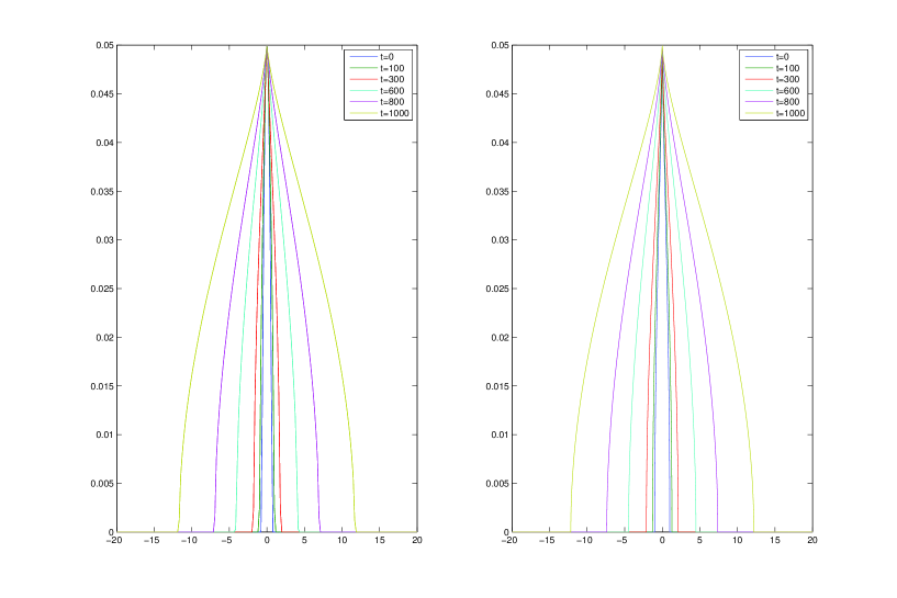
Figure 1: A generic solution and the asymptotic profile for Eq. (1.1) in dimension $N=1$, with $m=3$.

5 Further extensions, comments and open problems

In this final section we extend some results and state some open problems related to the present work. In particular, we discuss the large time behavior for non-radial initial data in dimension $N=1$.

1. The linear case $m=1$. This case is easy, since it can be directly transformed into the standard Heat Equation (2.5) by the change of variable (2.4). Thus, we get from [12] that the large time behavior is given by the same asymptotic profiles as there, but in our case with $N\in\{1,2\}$, namely (omitting the exact regularity assumptions on $u_{0}$, which are the same as in [12, Theorems 1.1 and 1.2])

$\bullet$ If $u_{0}(0)=0$, we have

$$\lim\limits_{t\to\infty}t^{1/2}\left\|u(\cdot,t)-\frac{M_{u_{0}}}{\omega}F(\cdot,t)\right\|_{\infty}=0,$$ (5.1)

where $\omega=2\pi$ if $N=2$ and $\omega=1$ if $N=1$,

$$M_{u_{0}}:=\int_{\mathbb{R}^{N}}|x|^{-N}u_{0}(x)\,dx<\infty,$$

and

$$F(x,t):=\left\{\begin{array}[]{ll}\frac{1}{\sqrt{4\pi t}}G\left(\frac{\log|x|+(N-2)t}{2\sqrt{t}}\right),\quad G(\xi)=e^{-\xi^{2}},&{\rm for}\ |x|\neq 0,\\ 0,&{\rm for}\ x=0,\end{array}\right.$$ (5.2)

$\bullet$ If $u_{0}(0)=K>0$, we have

$$\left\|u(\cdot,t)-\frac{K}{2}E(\cdot,t)\right\|_{\infty}=O(t^{-1/2}),\quad{\rm as}\ t\to\infty,$$ (5.3)

where

$$E(x,t):=\left\{\begin{array}[]{ll}{\rm erfc}\left(\frac{\log|x|+(N-2)t}{2\sqrt{t}}\right),\quad{\rm erfc}(\xi)=\frac{2}{\sqrt{\pi}}\int_{\xi}^{\infty}e^{-\theta^{2}}\,d\theta,&{\rm for}\ |x|\neq 0,\\ K,&{\rm for}\ x=0.\end{array}\right.$$ (5.4)

These statements are given here only at a formal level, for a rigorous analysis see [12].

2. Non radially symmetric solutions. This is a natural question, as on the one hand, our techniques (specially in dimension $N=2$) depend strongly on the symmetry of the solutions, and on the other hand, in the linear case the authors were able to show that the evolution do not symmetrize in the large time behavior (see [12, Introduction] for a counterexample). In dimension $N=1$, one can get a full result for general data $u_{0}$ by noticing that the origin is disconnecting the real line. Thus, if $u_{0}$ is a general data, we can define the radially symmetric data

$$u_{0}^{+}(x)=\left\{\begin{array}[]{ll}u_{0}(x),&{\rm for}\ x\geq 0,\\ u_{0}(-x),&{\rm for}\ x<0,\end{array}\right.\qquad u_{0}^{-}(x)=\left\{\begin{array}[]{ll}u_{0}(x),&{\rm for}\ x\leq 0,\\ u_{0}(-x),&{\rm for}\ x>0,\end{array}\right.$$

and respectively, the corresponding radially symmetric solutions $u^{+}(x,t)$, $u^{-}(x,t)$. To give an example, suppose that $u_{0}(0)=K>0$ (the case $u_{0}(0)=0$ is similar), then $u_{0}^{+}(0)=u_{0}^{-}(0)=K$, whence, by Theorem 1.4, there exist $x_{0}^{+}$ and $x_{0}^{-}\in\mathbb{R}$ such that

$$\lim\limits_{t\to\infty}\|u^{+}(\cdot,t)-U_{x_{0}^{+}}(\cdot,t)\|_{\infty}=\lim\limits_{t\to\infty}\|u^{-}(\cdot,t)-U_{x_{0}^{-}}(\cdot,t)\|_{\infty}=0.$$ (5.5)

Moreover, since $u(0,t)=K$ for any $t>0$, solving the Cauchy problem with $u_{0}$ reduces to solving two Dirichlet problems on the two half-lines with boundary data $K>0$ and then matching the two solutions. This shows that

$$u(x,t)=\left\{\begin{array}[]{ll}u^{+}(x,t),&{\rm for}\ x\geq 0,\\ u^{-}(x,t),&{\rm for}\ x<0,\end{array}\right.$$ (5.6)

for any $(x,t)\in\mathbb{R}\times(0,\infty)$. We thus infer from (5.5) and (5.6) that

$$\lim\limits_{t\to\infty}\|u(\cdot,t)-U(\cdot,t)\|_{\infty}=0,\qquad U(x,t)=\left\{\begin{array}[]{ll}U_{x_{0}^{+}}(x,t),&{\rm for}\ x\geq 0,\\ U_{x_{0}^{-}}(x,t),&{\rm for}\ x<0,\end{array}\right.$$ (5.7)

which is the desired large time behavior.

However, in dimension $N=2$ the previous argument does not work, and we do not have for the moment an answer to the question whether general data also lead to radially symmetric profiles or not. We leave this as an open problem. Our conjecture is that non-radial asymptotic behavior should appear, in line with [12].

3. Open problems for other $\gamma$ and $m$. In the papers [18, 27], a connection between equations such as (1.1) in dimension $N=1$ (but with general density $\varrho(x)=|x|^{-\gamma}$ for $\gamma=(3m+1)/2m$) and some Fisher-KPP type equations is done. As a byproduct, the authors deduce that the large time behavior in their cases is given by self-similar, dipole-type profiles. This is in itself a very interesting result, but does not interact with ours, since $\gamma=2$ implies $m=1$, while the transformation in [18] only applies to $m>1$. However, having these works as starting point, we raise the open problem of studying the large time behavior for the general form of (1.1), that is

$$|x|^{-\gamma}\partial_{t}u(x,t)=\Delta u^{m}(x,t),$$

where the most interesting case is when $2<\gamma$ and $m>1$. It seems to us that for the general case $(\gamma,m)$, there is no useful mapping to another well-known equation; such mappings may exist, but only for some special relations between $\gamma$ and $m$.

References

- [1] N. Alikakos, R. Rostamian, On the uniformization of the solutions of the porous medium equation in , Isralel J. Math., 47 (1984), no. 4, 270-290.
- [2] E. DiBenedetto, A. Friedman, Holder estimates to nonlinear degenerate parabolic systems, J. Reine Angew. Math., 357 (1985), 1-22.
- [3] C. J. van Duijn, J. M. de Graaf, Large time behavior of solutions of the porous medium equation with convection, J. Differential Equations, 84 (1990), no. 1, 183-203.
- [4] C. J. van Duijn, L. A. Peletier, Asymptotic behavior of solutions of a nonlinear diffusion equation, Arch. Rational Mech. Anal., 65 (1977), 363-377.
- [5] M. Escobedo, J. L. Vázquez, E. Zuazua, Asymptotic behavior and source-type solutions for a diffusion-convection equation, Arch. Rational Mech. Anal., 124 (1993), 43-65.
- [6] D. Eidus, The Cauchy problem for the nonlinear filtration equation, J. Differential Equations, 84 (1990), 309-318.
- [7] D. Eidus, S. Kamin, The filtration equation in a class of functions decreasing at infinity, Proc. Amer. Math. Society, 120 (1994), no. 3, 825-830.
- [8] V. A. Galaktionov, S. Kamin, R. Kersner, J. L. Vázquez, Intermediate asymptotics for a nonhomogeneous nonlinear heat equation, Tr. Semin. im. I. G. Petrovskogo, 23 (2003), 61-92, translation in J. Math. Sci. 120 (2004), no. 3, 1277-1294.
- [9] G. Grillo, M. Muratori, F. Punzo, On the asymptotic behavior of solutions to the fractional porous medium equation with variable density, Discrete Cont. Dyn. Syst., 35 (2015), no. 12, 5927-5962.
- [10] R. Kersner, A. Tesei, Well-posedness of initial value problems for singular parabolic equations, J. Differential Equations, 199 (2004), no. 1, 47-76.
- [11] R. Iagar, G. Reyes, A. Sánchez, Radial equivalence of nonhomogeneous nonlinear diffusion equations, Acta Appl. Math., 123 (2013), 53-72.
- [12] R. Iagar, A. Sánchez, Asymptotic behavior for the heat equation in nonhomogeneous media with critical density, Nonl. Anal., 89 (2013), 24-35.
- [13] R. Iagar, A. Sánchez, Large time behavior for a porous medium equation in a nonhomogeneous medium with critical density, Nonl. Anal, 102 (2014), 224-241.
- [14] S. Kamin, G. Reyes, J. L. Vázquez, Long time behavior for the inhomogeneous PME in a medium with rapidly decaying density, Discrete Contin. Dyn. Syst. 26 (2010), no. 2, 521-549.
- [15] S. Kamin, P. Rosenau, Propagation of thermal waves in an inhomogeneous medium, Comm. Pure Appl. Math, 34 (1981), no. 6, 831-852.
- [16] S. Kamin, P. Rosenau, Nonlinear thermal evolution in an inhomogeneous medium, J. Math. Phys., 23 (1982), no. 7, 1385-1390.
- [17] S. Kamin, P. Rosenau, Thermal waves in an absorbing and convecting medium, Phys. D., 8 (1983), no. 1-2, 273-283.
- [18] S. Kamin, P. Rosenau, Emergence of waves in a nonlinear convection-reaction-diffusion equation, Adv. Nonlinear Stud, 4 (2004), no. 3, 251-272.
- [19] Ph. Laurençot, F. Simondon, Source-type solutions to porous medium equations with convection, Commun. Appl. Anal., 1 (1997), no. 4, 489-502.
- [20] Ph. Laurençot, F. Simondon, Long-time behavior to porous medium equations with convection, Proc. Roy. Soc. Edinburgh Sect. A, 128 (1998), no. 2, 315-336.
- [21] E. S. Nieto, G. Reyes, Asymptotic behavior of the solutions of the inhomogeneous porous medium equation with critical vanishing density, Commun. Pure Appl. Anal., 12 (2013), no. 2, 1123-1139.
- [22] S. Osher, J. Ralston, stability of traveling waves with application to convective porous media flow, Comm. Pure Appl. Math., 35 (1982), 737-749.
- [23] L. A. Peletier, Asymptotic behavior of solutions of the porous media equation, SIAM J. Appl. Math, 21 (1971), 542-551.
- [24] G. Reyes, J. L. Vázquez, The Cauchy problem for the inhomogeneous porous medium equation, Network Heterog. Media 1 (2006), no. 2 337-351.
- [25] G. Reyes, J. L. Vázquez, The inhomogeneous PME in several space dimensions. Existence and uniqueness of finite energy solutions, Commun. Pure Appl. Anal., 7 (2008), no. 6, 1275-1294.
- [26] G. Reyes, J. L. Vázquez, Long time behavior for the inhomogeneous PME in a medium with slowly decaying density, Commun. Pure Appl. Anal., 8 (2009), no. 2, 493-508.
- [27] P. Rosenau, Reaction and concentration dependent diffusion model, Phys. Rev. Let., 88 (2002), no. 19, 194501-4.
- [28] A. F. Tedeev, The interface blow-up phenomenon and local estimates for doubly degenerate parabolic equations, Appl. Anal., 86 (2007), no. 6, 755-782.
- [29] J. L. Vázquez, The interfaces of one-dimensional flows in porous media, Trans. Amer. Math. Soc., 285 (1984), no. 2, 717-737.
- [30] J. L. Vázquez, Asymptotic behavior for the porous medium equation posed in the whole space. Dedicated to Philippe Benilan, J. Evol. Equ. 3 (2003), no. 1, 67-118.
- [31] J.L. Vázquez, The Porous Medium Equation. Mathematical Theory, Oxford Math. Monographs, Oxford Univ. Press, Oxford, 2007.