Galileon Higgs Vortices

Abstract

Vortex solutions are topologically stable field configurations that can play an important role in condensed matter, field theory, and cosmology. We investigate vortex configuration in a 2+1 dimensional Abelian Higgs theory supplemented by higher order derivative self-interactions, related with Galileons. Our vortex solutions have features that make them qualitatively different from well-known Abrikosov–Nielsen-Olesen configurations, since the derivative interactions turn on gauge invariant field profiles that break axial symmetry. By promoting the system to a 3+1 dimensional string configuration, we study its gravitational backreaction. Our results are all derived within a specific, analytically manageable system, and might offer indications for understanding Galileonic interactions and screening mechanisms around configurations that are not spherically symmetric, but only at most cylindrically symmetric.

1 Introduction

Exact solutions to classical equations of motion offer glimpses on the non-perturbative structure of a given field theory, and can have important physical applications. Vortex solutions (Abrikosov abrvortex , Nielsen-Olesen Nielsen:1973cs ) are a good example since they play an essential role in the physics of superfluidity and superconductivity (see for example Donnelly ), and might exist in our 3+1 dimensional universe in the form of cosmic strings (see e.g. Vilenkin:2000jqa ). In a covariant Abelian Higgs theory, Nielsen-Olesen (NO) vortex solutions are axially symmetric field configurations of finite energy, characterised by couplings to the Higgs scalar and the electromagnetic vector field. They support a non-vanishing magnetic flux, and spontaneously break the Abelian gauge symmetry out of the vortex core. See e.g. Weinberg:2012pjx ; Dunne:1998qy for excellent textbook discussions on topological solutions in field theories.

In this paper, we ask what happens when the standard Abelian Higgs action is modified by adding higher order, gauge invariant derivative self-interactions for the Higgs field. For this aim, we focus on exploring vortex configurations in a Higgs model in $2+1$ dimensions, supplemented by derivative Higgs self-interactions related with Galileons Hull:2014bga .

Our motivations are the following:

• In the context of scalar tensor theories of gravity, or massive gravity, theories with Galileonic symmetries Nicolis:2008in have received much attention. They enjoy powerful non-renormalization theorems Nicolis:2004qq ; Nicolis:2008in , and offer good control of strongly coupled regimes that realise a Vainshtein mechanisms to screen scalar fifth forces and to raise the effective cut-off of the theory (see e.g. Brax:2013ida ; Babichev:2013usa for reviews) . Much of the analytic studies have focussed on spherically symmetric configurations, since the relevant field equations become algebraic Babichev:2012re ; Sbisa:2012zk ; Koyama:2013paa . On the other hand, it is interesting and important to ask what happens to the Vainshtein mechanism for less symmetric cases, as for cylindrical configurations (see e.g. Bloomfield:2014zfa for a preliminary study on this respect that neglects gravity backreaction, or the slowly rotating solutions discussed in Chagoya:2014fza ). The theory we consider is simpler than systems involving gravity, so it allows us to address analytically the problem of finding configurations in axially symmetric set-ups. Some of the relevant equations of motion are algebraic, making the analysis particularly straightforward. At the same time, the action is sufficiently non-linear to lead to new properties that are absent for the NO vortex, and that might be shared with systems where gravity is important.

• For Galileon symmetric theories, an analogue of Derrick theorem applies, preventing the existence of vortex configurations of finite energy in systems with scalar derivative self-interactions only Endlich:2010zj (see also Padilla:2010ir ). Recall that in the standard case of a theory of scalar fields with non-derivative interactions, the classical Derrick theorem Derrick:1964ww states that no finite energy vortex solutions exist. This conclusion can be circumvented by adding more structure to the theory, for example gauging the system by introducing vector fields with appropriate couplings and asymptotic behaviour. In this work, we are interested in a theory characterized by a Mexican hat Higgs potential; additionally, it contains higher order Higgs derivative self-interactions related with Galileons, and being gauged it couples the Higgs to a vector field Hull:2014bga . In such a framework, it is natural to ask whether the new Higgs derivative interactions qualitatively modify the structure of NO vortex, leading to novel effects that is worth exploring.

Starting from these motivations, we add higher order, derivative self-interactions to the standard Abelian Higgs Lagrangian. Such interactions have been first introduced in Hull:2014bga for providing a Higgs mechanism to spontaneously break the gauge symmetry through vector Galileon interactions Tasinato:2014eka ; Heisenberg:2014rta . They are ghost free, and in a suitable high energy limit they enjoy Galilean symmetries that might protect their structure. We dub this system Galileon Higgs model .

Within this framework, we are able to determine vortex solutions characterised by topologically conserved winding numbers. They have features that make them qualitatively different from the NO vortex. The derivative non-linear interactions necessarily turn on a new gauge invariant radial vector component. This radial component violates a reflection symmetry around one of the axis of the Cartesian coordinates, and leads to configurations that additionally break the axial symmetry of the configuration. Interestingly, some of the equations of motion reduce to quadratic algebraic equations, making our analysis particularly straightforward.

Figure 1 provides a graphical anticipation of our results: we show the gradient of the phase of the scalar field for the NO solution (left) and our Galileon Higgs vortex configuration (right) in a plane with Cartesian coordinates $(x_{1},\,x_{2})$. The violation of a reflection symmetry $x_{1}\to-x_{1}$ is manifest, and axial symmetry is broken since surfaces of constant scalar phase are not invariant under rotation of the central axis. Although in Fig 1 we focus on the Higgs phase, as we will discuss the same effect is manifest when discussing quantities that are gauge invariant.

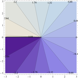
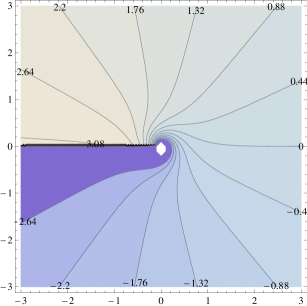
Figure 1: A representative example of the gradient of the Higgs phase for the Nielsen-Olesen vortex solution (left) and an approximate solution for the Galileonic vortex (right), plotted in the $x$-$y$ plane. The lines correspond to constant values for the Higgs phase.

Interestingly, the equation of motion for the radial vector component is a quadratic algebraic equation, and for some parameter choice its roots can become complex. This implies that the vortex solution ceases to exist in a region surrounding the origin of the radial coordinate, leading to a ‘thick’ singularity. We will develop a geometric understanding of this non-linear effect, and we will discuss some of its physical consequences.

It is also possible to study the backreaction of the system when coupling it with gravity. The new gauge invariant field profiles excite new components of the energy momentum tensor, that need to switch on appropriate metric components in order to satisfy Einstein equations. On the other hand, we show that field dependent coordinate transformations exist, that ‘adapt’ the geometry to our special vortex profile, and that make the resulting space-time manifestly axially symmetric.

2 A review: Vortex in the Abelian Higgs model

2.1 The Abelian-Higgs system

The Abelian Higgs Lagrangian is a U(1) gauge invariant system describing a massless gauge field, $A_{a}$, and a self interacting complex scalar field $\Phi$. Within a mostly minus signature convention, it is given by

$$\mathcal{L}_{AH}[\Phi,A_{a}]=(D_{a}\Phi)^{\dagger}D^{a}\Phi-\frac{1}{4}F_{ab}F^{ab}-\frac{\lambda}{4}\left(\Phi^{\dagger}\Phi-\eta^{2}\right)^{2},$$ (1)

where $D_{a}=\partial_{a}+ieA_{a}$ and $F_{ab}=D_{a}A_{b}-D_{b}A_{a}$. Although our discussion can be extended to four space-time dimensions, we restrict ourselves to 2+1 dimensions labeled by $(t,\,x_{1},\,x_{2})$. Thus the mass dimensions of the quantities above are $[\Phi\Phi^{\dagger}]=[e^{2}]=[\lambda]=[\eta^{2}]=[A^{2}]=1$. We will come back later to the Lagrangian in the form (1), but in order to present vortex configurations it is useful to take a shortcut by introducing the Ansatz

$$\Phi(x^{\alpha}) =\eta X(x^{\alpha})e^{i\chi(x^{\alpha})},$$ (2a)

$$A_{a}(x^{\alpha}) =\frac{1}{e}\left[\hat{A}_{a}(x^{\alpha})-\partial_{a}\chi(x^{\alpha})\right],$$ (2b)

where the new fields are all real and have mass dimensions $[\hat{A}_{a}]=1$ and $[X]=[\chi]=0$. The Lagrangian is invariant under a U(1) gauge transformation

$$\Phi\to\Phi e^{i\xi}\hskip 28.45274pt{\text{and}}\hskip 28.45274ptA_{a}\to A_{a}-e^{-1}\partial_{a}\xi,\,$$ (3)

for an arbitrary function $\xi$. The fields $X,$ and $\hat{A}_{a}$ introduced in eq. (2) are invariant under such a transformation.

The advantage of using Ansatz (2) is that $\chi$ drops out from the Lagrangian, that rewrites

$$\mathcal{L}_{AH}[X,\hat{A}_{a}]=\eta^{2}\partial_{a}X\partial^{a}X+\eta^{2}X^{2}\hat{A}_{a}\hat{A}^{a}-\frac{1}{4e^{2}}F_{ab}F^{ab}-\frac{\lambda\eta^{4}}{4}\left(X^{2}-1\right)^{2},$$ (4)

where $F_{ab}=\partial_{a}\hat{A}_{b}-\partial_{b}\hat{A}_{a}$. In this way the gauge invariant, physical degrees of freedom of the model have been extracted. The corresponding equations of motion are

$$\Box X-X\hat{A}_{a}\hat{A}^{a}+\frac{\lambda\eta^{2}}{2}\left(X^{2}-1\right)X =0,$$ (5a)

$$\partial_{a}F^{ab}+2e^{2}\eta^{2}X^{2}\hat{A}^{b} =0.$$ (5b)

We can identify two mass scales in these equations. The scalar equation contains $\sqrt{2}m_{X}=\sqrt{\lambda}\eta$, while the last term in the vector equation contains a mass associated to the vector field, $m_{V}=\sqrt{2}e\eta$. As we will see next, the mass scales $m_{X}$ and $m_{V}$ control the field profiles, and therefore the localization properties of the vortex.

2.2 The Nielsen-Olesen vortex

The vortex is a solution to gauge theories with scalar fields first studied by Abrikosov abrvortex , and Nielsen and Olesen Nielsen:1973cs . This solution describes a vortex-like object carrying a localized magnetic flux in its core. The size of the core depends on the mass scales of the theory, i.e. on the mass of the scalar and gauge fields.

Some simplifying assumptions can be done. First, $A_{0}$ is not a propagating degree of freedom, and it is consistent to set $A_{0}=0$ since this quantity appears at least quadratically in the Lagrangian. Furthermore, only static configurations are considered. Using Cartesian coordinates for the spatial part of the metric, the energy functional for such configurations is given by

$$\mathcal{E}_{AH}=\int d^{2}x\left[\frac{1}{2}B^{2}+|\vec{D}\Phi|^{2}+\frac{\lambda}{4}(|\Phi|^{2}-\eta^{2})^{2}\right],$$ (6)

where $B=-F_{12}=\partial_{x_{2}}A_{x_{1}}-\partial_{x_{1}}A_{x_{2}}$, and $\vec{D}$ has for components the spatial parts of $D_{a}$. Axial coordinates, that we use more frequently, are defined as usual as

$$r = \sqrt{x_{1}^{2}+x_{2}^{2}}\hskip 28.45274pt,\hskip 28.45274pt\theta\,=\,\arctan\left[\frac{x_{2}}{x_{1}}\right].$$ (7)

The integral (6) spans over the entire space, therefore in order to keep the energy finite we require the potential of the scalar field to vanish for large $r$, thus $|\Phi|^{2}=\eta^{2}$ asymptotically, or equivalently $X\to 1$ as $r\to\infty$.

Indeed the potential minimum is isomorphic to a circle and has solutions characterised by the phase $\chi$, $\Phi=\eta e^{i\chi}$. Asymptotically, $\chi$ defines a mapping from a circle of radius $r$ in real space to a circle of radius $\eta$ in the complex plane. Mappings from one circle to $N-$circles are described by

$$\chi=N\theta\,,$$ (8)

where $\theta$ is the polar angle and the integer $N$ is the winding number. It counts the number of circles in complex space corresponding to a circle at spatial infinity. The winding number is a topological invariant, in the sense that the asymptotic value of the phase (8) cannot be modified by a gauge transformation that is regular everywhere. Hence the winding number characterises different classes of finite energy solutions.

One further asymptotic condition that we must impose to keep the energy finite is $D_{a}\Phi=0$ at $r\to\infty$. This requirement can be fulfilled thanks to the coupling of the scalar with the vector field, and it is crucial to avoid Derrick theorem. Using the definition of $D_{a}$, this asymptotic condition implies

$$A_{a}\sim\frac{i}{e}\partial_{a}\ln\Phi\sim-\frac{N}{e}\partial_{a}\theta,$$ (9)

as $r\to\infty$. Hence the vector field profile compensates for the scalar contribution at large $r$, keeping the energy finite Weinberg:2012pjx . Once we know the asymptotic form of the gauge field for a vortex, we can readily compute its magnetic flux by integrating over a loop at $r\to\infty$,

$${\text{Flux}}\,=\,e\int d^{2}xB=-e\oint A_{i}dx^{i}=2\pi N,$$ (10)

then the flux is an integer multiple of $2\pi$. This result depends only on the asymptotic behaviour of the fields and therefore it holds also for the model of Galileon Higgs that we use in the next section.

In addition to the asymptotic conditions at $r\to\infty$, we also need

$$A_{a}(r\to 0)=0,\ \ X(r\to 0)=0$$ (11)

to guarantee the regularity of the solutions at the origin. As (4) shows, when we use the Ansatz (2), the Higgs phase $\chi$ drops out and the physical degrees of freedom of the theory are only in $\hat{A}_{a}$ and $X$. In consequence, at this point we are free to fix the phase to depend on $\theta$ only, as $\chi=N\theta$. After making this choice, we are no longer free to perform a gauge transformation to remove the radial component of $A_{r}$ (the longitudinal mode), though. Nevertheless, for the system we consider in this section, it is consistent to assume that the component $A_{r}$ vanishes.

More precisely, in order to uniquely determine the vortex solution we impose the following two conditions Weinberg:2012pjx :

1. Rotational symmetry, in the sense that the effects of spatial rotations can be compensated by a gauge transformation that is uniform all over the space.

2. Invariance under reflection about the $x_{1}$ axis, accompanied by complex conjugation of the scalar field. Such discrete symmetry requires that the vector components obey

   $${A}_{1}(r,\,\theta)=-{A}_{1}(r,-\theta)\hskip 28.45274pt{\text{ and}}\hskip 28.45274pt{A}_{2}(r,\,\theta)={A}_{2}(r,-\theta).$$ (12)

We introduce the following Ansatz for the gauge invariant vector components (recall that vector gauge invariant components are labeled with a hat)

$$\hat{A}_{i}\,dx^{i}=\left[-\epsilon_{ij}\,\frac{{x_{j}}}{r}\,\hat{A}_{\theta}(r)+\frac{x_{i}}{r}\,\hat{A}_{r}(r)\right]\,dx^{i}.$$ (13)

The previous requirements implies that $X$, $\hat{A}_{\theta}$, and $\hat{A}_{r}$ depend on $r$ only. To make Ansatz (13) compatible with (12) accompanied by a complex conjugation of the scalar field, the second requirement imposes that $\partial_{r}\chi\,=\,0$, and at the same time $\hat{A}_{r}\,=\,{A}_{r}\,=\,0$. This condition is compatible with the equations of motion, since $\hat{A}_{r}$ appears at least quadratically in the action (this is a major difference with respect to the Galileon Higgs theory that we will discuss in the next section).

Within this Ansatz, the four equations given by (5) are reduced to two coupled equations for the fields $X$, $\hat{A}_{\theta}$:

$$r\eta^{4}\lambda X\left(1-X^{2}\right)-\frac{2\eta^{2}\hat{A}_{\theta}^{2}X}{r}+2\eta^{2}X^{\prime}+2r\eta^{2}X^{\prime\prime} =0,$$ (14a)

$$-2e^{2}r\eta^{2}\hat{A}_{\theta}X^{2}-\hat{A}_{\theta}^{\prime}+r\hat{A}_{\theta}^{\prime\prime} =0.$$ (14b)

Exact solutions to these equations can not be expressed in terms of standard functions; however several numerical and approximate results both for the Abelian Higgs model and generalizations exist (see e.g. Lake:2010wt, ; Kawabe:1997ua, ; Jatkar:2000ei, ).

Figure 2: $\hat{A}_{\theta}$ (green) and $X$ (blue) for Nielsen-Olesen vortices with $N=1$ and $\lambda=2e^{2}$. For the solid lines $\lambda=\eta=1$, while for the dashed lines $\lambda=\eta=0.8$. By changing these parameters we are changing the masses of the scalar and vector fields, and this modifies the width of the vortex core.

In Fig. 2 we show the representative example of a numerical solution to the equations (14), it corresponds to a vortex with winding number $N=1$. Notice that although the equations of motion do not depend explicitly on the vorticity, the boundary conditions do so (see eq. (9)). In this sense, the winding number does control the solutions. The profile for the scalar and magnetic fields can be understood as follows Weinberg:2012pjx . Since there is non-vanishing vorticity, there must be regions where the magnetic field is different from zero. The gauge field acquires a mass when the scalar field is non-vanishing. Hence it is energetically favoured for the magnetic field to be concentrated in a region near the origin, where the scalar field acquires a value close to zero; moreover, rendering this region thicker reduces the magnetic energy contribution. Contrasting this effect, and favouring a smaller vortex core, is the fact that it costs energy for the scalar to be away from the minimum of its Mexican hat potential. The relative strength of these two competing effects is determined by $\lambda/e^{2}$.

2.3 Boundedness of the Hamiltonian and the BPS bound

Another important property of NO configurations is the existence of a particular point in the parameter space known as the Bogomol’nyi point Bogomolny:1975de , or alternatively as the BPS bound, given by $\lambda=2e^{2}$. To see what makes this point special we need to consider the energy functional for static configurations:

$$\mathcal{E}_{AH}=\int d^{2}x\left[\frac{1}{2}B^{2}+|\vec{D}\Phi|^{2}+\frac{\lambda}{4}(|\Phi|^{2}-\eta^{2})^{2}\right].$$ (15)

Noticing that $|\vec{D}_{\Phi}|^{2}=|(D_{1}\pm iD_{2})\Phi|^{2}\mp eB|\Phi|^{2}\pm 2\partial_{\{i}J_{j\}}$, where $2iJ_{j}=\Phi^{\dagger}D_{j}\Phi-\Phi(D_{j}\Phi)^{\dagger}$, making a ‘complete the square’ argument and dropping boundary terms, the energy functional becomes

$$\mathcal{E}_{AH}=\int d^{2}x\left[\frac{1}{2}\left(B\mp e(|\Phi|^{2}-\eta^{2})\right)^{2}+|D_{\pm}\Phi|^{2}+\left(\frac{\lambda}{4}-\frac{e^{2}}{2}\right)\left(|\Phi|^{2}-\eta^{2}\right)^{2}\mp e\eta^{2}B\right].$$ (16)

This expression shows that it is bounded from below. The potential term vanishes if $\lambda=2e^{2}$. The other conditions to minimize the energy functional are

$$D_{\pm}\Phi =0,$$ (17a)

$$B =\pm e\left(|\Phi|^{2}-\eta^{2}\right).$$ (17b)

These are known as the BPS self-duality equations Prasad:1975kr ; Coleman:1976uk . By considering axially symmetric configurations these equations reduce to (14) with $\lambda=2e^{2}$.

3 The vortex in presence of Galileon Higgs interactions

3.1 The Higgs model including higher order derivative self-interactions

The Abelian Higgs model defined by Lagrangian (1) can be extended including non-linear derivative self-interactions of the gauge field, which can be relevant in the context of vector-field models for dark energy (see, e.g. Clifton:2011jh for a general review). Such derivative interactions are ghost free and gauge invariant; since they involve covariant derivatives they couple the Higgs to gauge fields. They have been introduced in Hull:2014bga as a way for Higgsing the Abelian symmetry breaking model of vector Galileons Tasinato:2014eka ; Heisenberg:2014rta ; Tasinato:2014mia . Regardless of this motivation, they can be seen as ghost-free derivative extensions of the Abelian Higgs model, related with Galileon systems in an appropriate decoupling limit (as we will review below). This connection with Galileons can be useful for analysing the (non-)renormalization properties of our derivative interactions under quantum corrections. This is an issue outside the scope of this work, and that we leave for further studies.

In three space-time dimensions only two of the three new proposed operators can be defined, and in static situations only the lowest dimensional of these operators is different from zero. This operator, which we call $\mathcal{L}_{6}$ in reference to its mass dimension, is given by

$$\mathcal{L}_{\mathrm{6}} = -\frac{1}{\Lambda^{3}}\,\varepsilon^{ca_{1}a_{2}}\varepsilon_{cb_{1}b_{2}}\,\left[\,\alpha_{(6)}L_{a_{1}}^{\,b_{1}}P_{a_{2}}^{\,b_{2}}+\beta_{(6)}L_{a_{1}}^{\,b_{1}}Q_{a_{1}}^{\,b_{2}}\,\right],$$ (18)

where $\Lambda$ has dimensions of mass and $\alpha_{(6)}$ and $\beta_{(6)}$ are dimensionless; all these parameters are constant. $\varepsilon_{abc}$ is a totally antisymmetric tensor in three dimensions with $\varepsilon_{123}=1$, and the gauge invariant operators $P_{ab}$ and $Q_{ab}$ are expressed in terms of the Higgs covariant derivatives by

$$L_{{a}{b}} \equiv\frac{1}{2}\left[({D}_{{a}}\Phi)^{*}({D}_{{b}}\Phi)+({D}_{{b}}\Phi)^{*}({D}_{{a}}\Phi)\right]\,,$$ (19a)

$$P_{{a}{b}} \equiv\frac{1}{2}\left[\Phi^{*}{D}_{{a}}{D}_{{b}}\Phi+\Phi\,\left({D}_{{a}}{D}_{{b}}\Phi\right)^{*}\right]\,,$$ (19b)

$$\,Q_{{a}{b}} \equiv\frac{i}{2}\left[\Phi\left({D}_{{a}}{D}_{{b}}\Phi\right)^{*}-\Phi^{*}{D}_{{a}}{D}_{{b}}\Phi\right]\,.$$ (19c)

These operators are symmetric as can be verified by expanding the gauge derivatives. Following the same route as in the previous section, we proceed to write down the Lagrangian in terms of the fields $X,\chi$ and $\hat{A}_{a}$. Using the ansatz (2) we write the previous operators in terms of the gauge invariant field $\hat{A}_{a}$ and the real scalar field $X$,

$$L_{{a}{b}} =\eta^{2}\partial_{{a}}X\partial_{{b}}X+\eta^{2}X^{2}\hat{A}_{{a}}\hat{A}_{{b}}\,,$$ (20a)

$$P_{{a}{b}} =\eta^{2}X\partial_{{a}}\partial_{{b}}X-\eta^{2}X^{2}\hat{A}_{{a}}\hat{A}_{{b}}\,,$$ (20b)

$$Q_{{a}{b}}\, =\frac{1}{2}\eta^{2}\,[\partial_{{a}}(X^{2}\hat{A}_{{b}})+\partial_{{b}}(X^{2}\hat{A}_{{a}})]\,.$$ (20c)

Notice that the phase $\chi$ does not appear in the previous expressions, as expected since all quantities are written in a gauge invariant form. For simplicity, we focus only in the part of the Lagrangian proportional to $\beta_{(6)}$ that depends on vector field derivatives, and that as we will discuss switches on new field profiles that we wish to investigate. Hence, making a rescaling and redefining $\beta_{(6)}=\Lambda^{3}\beta$ the Lagrangian $\mathcal{L}_{6}$ that we study is

$$\mathcal{L}_{6}[X,\hat{A}]=\beta\eta^{4}\left(\partial_{a}X\partial_{b}X+X^{2}\hat{A}_{a}\hat{A}_{b}\right)\left[\eta^{ab}\partial^{c}(X^{2}\hat{A}_{c})-\partial^{a}(X^{2}\hat{A}^{b})\right].$$ (21)

3.2 (Bi)galileons from decoupling limit

In this subsection, we review the connection between the Higgs derivative self-interactions that we consider, and Galileon theories, referring to Hull:2014bga for a more extensive discussion.

We first need to expand the Higgs around its vev: using our notation, this implies that we introduce the field $h$ as a perturbation around the $X=1$ Higgs vev:

$$X\,\equiv\,1+\frac{h}{\sqrt{2}}.$$ (22)

The total Lagrangian, expanded in terms of the field $h$ and the vector fields, reads

$${\cal L}_{tot} = -\frac{1}{4}F_{\mu\nu}F^{\mu\nu}-m_{A}^{2}\,\hat{A}^{2}-\tilde{\beta}\,\hat{A}_{\mu}\hat{A}^{\mu}\,\partial_{\rho}\hat{A}^{\rho}$$ (23)

$$-\frac{1}{2}\,(\partial h)^{2}-\frac{1}{2}\,m_{h}^{2}\,h^{2}\,-\frac{\sqrt{\lambda}\,m_{h}}{4}\,h^{3}\,-\frac{{\lambda}\,}{{16}}\,h^{4}-\sqrt{2}\,e\,m_{A}\,h\,\hat{A}_{\mu}\hat{A}^{\mu}-\frac{e^{2}}{2}\,h^{2}\,\hat{A}_{\mu}\hat{A}^{\mu}\,$$

$$+\frac{4\,e\,\tilde{\beta}}{3\,m_{A}}\,\left(\sqrt{2}\,h+\frac{3\,e}{2\,m_{A}}\,h^{2}\,+\frac{e^{2}}{\sqrt{2}\,m_{A}^{2}}\,h^{3}+\frac{e^{3}}{8\,m_{A}^{3}}\,h^{4}\right)\,\left(\hat{A}_{\mu}\,\hat{A}^{\nu}\,\partial_{\nu}\hat{A}^{\mu}-\hat{A}_{\mu}\,\hat{A}^{\mu}\,\partial_{\rho}\hat{A}^{\rho}\right)$$

$$+\frac{\tilde{\beta}}{3\,m_{A}^{2}}\,\left(1+\frac{\sqrt{2}\,e}{m_{A}}\,h+\frac{e^{2}}{2\,m_{A}^{2}}\,h^{2}\right)\left(\partial_{\mu}h\,\partial^{\nu}h\,\partial_{\nu}\hat{A}^{\mu}-\partial_{\mu}h\,\partial^{\mu}h\,\partial_{\rho}\hat{A}^{\rho}\right)\,,$$

with

$$m_{A} = e\,\eta\,,$$ (24a)

$$\tilde{\beta} = -\frac{3\,e^{3}\,\beta_{(6)}\,v^{4}}{2\Lambda^{4}}\,,$$ (24b)

$$m_{h} = \sqrt{\lambda}\,\eta\,.$$ (24c)

Such Lagrangian is gauge invariant; nevertheless the system exhibits spontaneous symmetry breaking, and it contains a mass for the Higgs field $h$ and the vector field, as well as various derivative interactions between the Higgs and the vector components. Since the vector is now massive, it propagates three degrees of freedom, two transverse and one longitudinal. We are now interested to exhibit a ‘decoupling limit’ where the only interactions left are the ones between the Higgs with itself and with the longitudinal component of the vector. We will learn that such interactions have a bi-Galileon structure.

In order to make such interactions more manifest, we introduce by hand a ‘Stückelberg’ field to identify more simply the vector longitudinal mode: whenever we meet a vector in the Lagrangian (23) we substitute it with

$$\hat{A}_{\mu}\,\to\,\hat{A}_{\mu}-\frac{\partial_{\mu}\,\hat{\pi}}{\sqrt{2}\,m_{A}}.$$ (25)

The theory acquires an additional gauge symmetry $A_{\mu}\to A_{\mu}+2m_{A}\,\omega$, $\pi\to\pi+\omega$. Choosing a gauge in which $\pi=0$ one recovers the original Lagrangian. The field $\pi$ plays the physical role of the vector longitudinal polarization.

Consider the decoupling limit

$$e\to 0\hskip 14.22636pt,\hskip 14.22636pt\lambda\to 0\hskip 14.22636pt,\hskip 14.22636pt\beta_{(6)}\to 0\hskip 14.22636pt,\hskip 14.22636pt\eta\to\infty\,\,,$$ (26)

such that

$$m_{A}\to 0\hskip 14.22636pt,\hskip 14.22636ptm_{h}\to 0\hskip 14.22636pt,\hskip 14.22636pt\tilde{\beta}\to 0\hskip 14.22636pt,\hskip 14.22636pt\frac{\tilde{\beta}}{m_{A}^{3}}\,=\,{\rm fixed}\,\equiv\,\frac{1}{\Lambda_{g}^{3}}\,\,,$$ (27)

where $\Lambda_{g}$ is a mass scale associated with the Galileon interactions. In order to have a correctly normalized kinetic term for the Stückelberg field $\pi$ (corresponding to the vector longitudinal polarization) we rescale it, and define $\pi=\hat{\pi}/(\sqrt{2}m_{A})$. Within the decoupling limit, $\hat{\pi}$ plays the role of Goldstone boson of the broken symmetry. In the limit (26, 27), when expressed in terms of the canonically normalized Goldstone field $\hat{\pi}$, the total Lagrangian ${\cal L}_{tot}$ reduces to

$${\cal L}_{tot}\,=\,-\frac{1}{4}F_{\mu\nu}F^{\mu\nu}-\frac{1}{\Lambda_{g}^{3}}\,\left(\partial_{\mu}\hat{\pi}\partial^{\mu}\hat{\pi}\right)\,\Box\hat{\pi}-\frac{1}{3\,\Lambda_{g}^{3}}\left(\partial_{\mu}h\,\partial^{\mu}h\,\Box\hat{\pi}-\partial_{\mu}h\,\partial^{\nu}h\,\partial_{\nu}\partial^{\mu}\hat{\pi}\right)\,.$$ (28)

Hence in this decoupling limit the Lagrangian acquires a bi-Galileon structure, since the Higgs itself acquires bi-Galileon couplings with the field $\hat{\pi}$, corresponding to the vector longitudinal polarization. Outside the decoupling limit, the Higgs couple with the transverse polarizations of the vector as well, and this fact allows the system to circumvent Derrick’s theorem and to find vortex solutions of finite energy.

3.3 Equations of motion for a vortex configuration

As for the Abelian-Higgs model, the phase $\chi$ – and the vorticity as well – do not appear explicitly in the equations of motion, that can be expressed in a gauge invariant form. At large $r$ we impose the phase to be asymptotically

$$\chi=N\theta,$$ (29)

so to equip the configuration with a topologically invariant winding number.

On the other hand, analogously to the case of the NO vortex, the degrees of freedom $\hat{A}_{a}$ and $X$ are aware of the value of the vorticity through the boundary conditions (9), which together with $|\Phi|^{2}=|\eta^{2}|$ guarantee that the static energy functional is finite since all the terms in the Lagrangian vanish asymptotically. Hence the same asymptotic conditions for a Nielsen-Olesen vortex in the Abelian Higgs model remain valid when $\mathcal{L}_{6}$ is turned on. The presence of the vector allows us to find finite energy vortex configurations. In terms of our Ansatz of eqs. (2) and (13), that we write again here

$$\Phi = \eta X(r)e^{i\chi}\,,$$ (30a)

$$A_{a}(x^{\alpha}) = \frac{1}{e}\left[\hat{A}_{a}(x^{\alpha})-\partial_{a}\chi(x^{\alpha})\right],$$ (30b)

$$\hat{A}_{i}\,dx^{i} = \left[-\epsilon_{ij}\,\frac{{x_{j}}}{r}\,\hat{A}_{\theta}(r)+\frac{x_{i}}{r}\,\hat{A}_{r}(r)\right]\,dx^{i},$$ (30c)

the asymptotic conditions required in order to get finite energy solutions are

$$\hat{A}_{\theta}\to 0,\ \ \hat{A}_{r}\to 0,\ \ X\to 1,$$ (31)

at $r\to\infty$. Additionally, in order to compensate for the scalar contributions to the energy density, recall that $A_{\theta}$ satisfies the asymptotic condition (9).

The equations of motion can be expressed in fully covariant form. However it is more convenient for our purposes to write $\mathcal{L}_{6}$ in terms of the components of Ansatz (30c)

$$\mathcal{L}_{6}= \frac{4\beta\eta^{4}}{r^{3}}X{}^{2}\left[r^{2}\hat{A}_{r}{}{}^{3}X{}^{2}+r\hat{A}_{\theta}{}{}^{2}X{}^{2}\hat{A}_{r}{}^{\prime}{}+\hat{A}_{r}{}{}\left(2\hat{A}_{\theta}{}{}^{2}X{}^{2}-r\hat{A}_{\theta}{}{}X{}^{2}\hat{A}_{\theta}{}^{\prime}{}+r^{2}X^{\prime}{}^{2}\right)\right],$$ (32)

and to compute the equations of motion explicitly by taking the variation of the action with respect to these components. In doing so we should be careful not to oversimplify things. In particular, since none of our fields depends on time we can, and we had, set the time component $\hat{A}_{0}$ equal to zero, but we cannot do the same for the radial component, $\hat{A}_{r}$, because (32) contains terms linear in $\hat{A}_{r}$ whose contribution to the equations of motion would be missing if we set $\hat{A}_{r}=0$.

As a consequence, the complete Lagrangian

$$\mathcal{L}_{AHG}=\mathcal{L}_{AH}+\mathcal{L}_{6},$$ (33)

leads to three independent equations of motion, expressed in terms of gauge invariant quantities:

$$r\eta^{4}\lambda X\left(1-X^{2}\right)-\frac{2\eta^{2}\hat{A}_{\theta}^{2}X}{r}+2\eta^{2}X^{\prime}+2r\eta^{2}X^{\prime\prime}$$

$$+16\beta\eta^{4}X^{3}\hat{A}_{r}\left[\hat{A}_{r}^{2}+\frac{2{}\hat{A}_{\theta}^{2}}{r^{2}}+\frac{{}\hat{A}_{\theta}^{2}\hat{A}_{r}^{\prime}{}}{r\hat{A}_{r}}-\frac{{}{}\hat{A}_{\theta}{}\hat{A}_{\theta}^{\prime}{}}{r}-\frac{{}\hat{A}_{r}^{\prime}{}X^{\prime}{}}{2X\hat{A}_{r}}-\frac{{}{}X^{\prime}{}^{2}}{2X^{2}}-\frac{{}{}X^{\prime\prime}{}}{2X}\right] =0,$$ (34a)

$$-2e^{2}r\eta^{2}\hat{A}_{\theta}X^{2}-\hat{A}_{\theta}^{\prime}+r\hat{A}_{\theta}^{\prime\prime}+12\beta e^{2}\eta^{4}X^{4}r\hat{A}_{\theta}\left[\frac{{}\hat{A}_{r}{}}{r}+{}\hat{A}_{r}^{\prime}{}+\frac{4{}\hat{A}_{r}{}X^{\prime}{}}{3X}\right] =0,$$ (34b)

$$-r\eta^{2}\hat{A}_{r}{}X{}^{2}+6\beta\eta^{4}X^{4}\left[\hat{A}_{r}^{2}+\frac{\hat{A}_{\theta}^{2}}{r^{2}}-\frac{\hat{A}_{\theta}{}\hat{A}_{\theta}^{\prime}{}}{r}-\frac{4{}\hat{A}_{\theta}^{2}X^{\prime}{}}{3Xr}+\frac{{}X^{\prime}{}^{2}}{3X^{2}}\right] =0.$$ (34c)

We reiterate that, as for the NO vortex, the phase and the vorticity do not appear in the equations of motion for our gauge invariant quantities; but they do determine the profile of the fields by means of the boundary conditions required to get finite energy solutions.

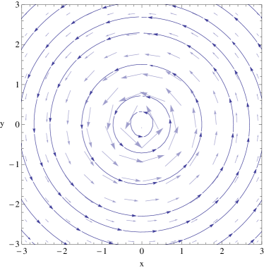
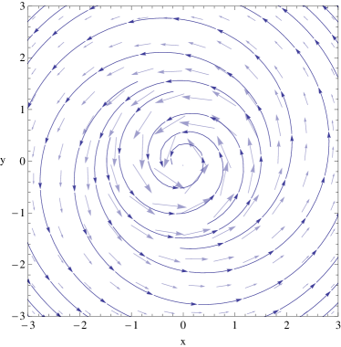
Figure 3: A representative example of the gauge invariant vector field $\hat{A}_{i}$ in Cartesian coordinates for a NO vortex (left) and for a Galileon Higgs vortex with $\beta=0.40$. Reflection invariance around a Cartesian axis is lost in the Galileon Higgs case.

The most interesting new feature of this set of equations is eq. (34c), the algebraic equation of motion for $\hat{A}_{r}$. For $\beta\neq 0$ this quadratic algebraic equation does not admit the solution $\hat{A}_{r}=0$. Instead the formal solution of this equation – compatible with our asymptotic conditions for vanishing asymptotic gauge fields – is

$$\hat{A}_{r}=\frac{r}{12\beta\eta^{2}X^{2}}\left[1-\sqrt{1-\left(\frac{12\beta\eta^{2}X^{2}}{r}\right)^{2}\,\left[\frac{\hat{A}_{\theta}}{r^{2}}(\hat{A}_{\theta}-r\hat{A}_{\theta}^{\prime}{})+\frac{X^{\prime}}{3X}\left(\frac{X^{\prime}{}}{X}-\frac{4\hat{A}_{\theta}^{2}}{r}\right)\right]}\right].$$ (35)

A non-vanishing $\hat{A}_{r}$ implies that we are violating the second requirement discussed in the previous section (in particular eq. (12)), hence we have a system that is not invariant under reflection around the $x_{1}$-axis, accompanied by a complex conjugation of the scalar field . The expression (35) for $\hat{A}_{r}$ can be substituted into eqs. (14a) and (14b) to find solutions for $X$ and $\hat{A}_{\theta}$. The solutions for $\hat{A}_{\theta}$, $\hat{A}_{r}$ can be included into the Ansatz (13) to obtain configurations for the gauge invariant components $\hat{A}_{1}$ and $\hat{A}_{2}$ in cartesian coordinates. Fig 3 shows a comparison of the profiles for $\hat{A}_{1}$ and $\hat{A}_{2}$ between NO and our vortex solution. The breaking of reflection symmetry is evident. We emphasize that in Fig 3 we are plotting gauge invariant, physical quantities. Our resulting vortex configurations do not switch on new electric fields, but nevertheless they locally modify the profiles for the Higgs and magnetic fields associated with NO solutions.

Notice that the configuration (35) contains a square root – being solution of a quadratic equation – hence for some choices of parameters a real solution for $\hat{A}_{r}$ might not exist in some regions of the radial coordinate. This fact is crucial for determining explicit solutions: we discuss this issue in what comes next.

3.4 Constructing Galileon Higgs vortex solutions

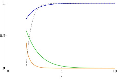
Figure 4: $\hat{A}_{\theta}$ (green), $\hat{A}_{r}$ (orange) and $X$ (blue) for a solution to eqs. (34) with $\beta=0.5$, $\lambda=1$ and $\eta=1$. This solution breaks down at the point where the argument of the square root in (35) (dashed line) drops to zero, showing that $\hat{A}_{r}$ does not admit a real solution for every set of parameters.

From the equations of motion for the AHG (Abelian Higgs Galileon) system, (34), we learn that although $\hat{A}_{r}$ does not have a dynamical equation of motion, it constrains the space of solutions to a subset for which $\hat{A}_{r}$ is real.

To see that this is indeed a constraint, we start considering an extreme, singular example in Fig. 4, where we present an explicit solution for our equations with $\beta=0.5$, selecting all the parameters and boundary conditions equal to those of a NO vortex. Although this solution is well behaved asymptotically, it breaks down before the vortex is formed. This occurs when $\hat{A}_{r}$ becomes complex, and is associated with the formation of a singularity. This example indicates clearly that in order to avoid singularities and find regular vortex solutions, we will have to control some features of our configuration.

To incorporate numerically the restriction imposed by $\hat{A}_{r}$, we allow the boundary conditions to vary until we find regular solutions across all the space. The system of equations that we solve is obtained by substituting (35) into (34a) and (34b). In Fig. 5 we show some of the solutions for different values of the coupling constant $\beta$. The boundary conditions for ‘large $r$’ are imposed at $r=20$. Note that $\hat{A}_{\theta}(r\to\infty)$ does not contain direct information about the vorticity since asymptotically such information cancels out in the gauge transformation (2b). However, at a finite but large $r$ the cancellation is not exact, and $\hat{A}_{\theta}$ is affected by the value of the vorticity. Conversely, a change in the boundary conditions for $\hat{A}_{\theta}$ and its derivative implies a change in the vorticity. In view of (2b) and (11), the change of vorticity becomes manifest at $r=0$, since $\hat{A}_{\theta}(r\to 0)=N$. This is indeed seen in Fig. 5, for example the vortices with $\beta=0.4$ and $\beta=0.5$ correspond approximately to $N=2$ and $N=3$ respectively. Increasing the vorticity, we find well-behaved solutions along the entire radial direction, even for larger values of the parameter $\beta$.

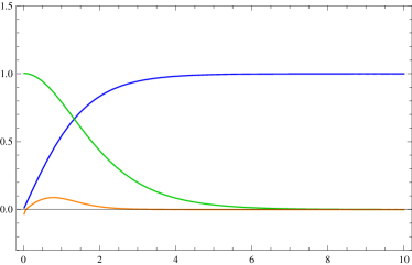
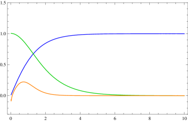
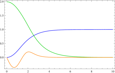
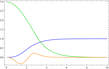
Figure 5: From top left to bottom right: $\beta=0.10\,\,(N=1),\,\beta=0.20\,\,(N=1),\,\beta=0.40\,\,(N=2)\text{ and }\,\beta=0.49\,\,(N=3)$. The fields shown are $\hat{A}_{\theta}$ (green), $\hat{A}_{r}$ (orange) and $X$ (blue). In all cases $\lambda=\eta=1$.

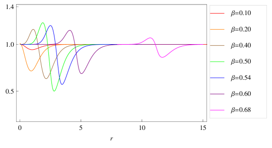
Figure 6: Argument of the square root that appears in $\hat{A}_{r}$, equation (35). The deviations from one correspond to regions where the non-linear effects can become large.

After analysing several numerical solutions with different boundary conditions, we conclude that there is a minimal vorticity to obtain complete solutions in the entire radial direction. Such minimal value increases with $\beta$ in a non-linear way. For example, for $0<\beta\lesssim 0.25$ any vorticity is allowed, for $0.25\lesssim\beta\lesssim 0.44$ the minimal vorticity is $N=2$ and for $0.44\lesssim\beta\lesssim 0.50$ the minimal vorticity is $N=3$.

The fact that increasing vorticity one finds real solutions over all the radial coordinate might be interpreted as follows. As explained at the end of Section 2.2, a vortex configuration is a balance between the tendencies of the magnetic field to get localized near the origin, and of the scalar field to lie on the minimum of its Mexican hat potential. Increasing vorticity changes the boundary conditions for the gauge field, and causes the vortex to become wider. When the Higgs derivative self-interactions are turned on, they can destabilise the aforementioned balance, since the new contributions of the gauge component $\hat{A}_{r}$ tend to make the the field profiles wider, up to a point where no static configurations exist. A way out is to increase the vorticity, since changing boundary conditions for the gauge field do allow for a wider vortex configurations, that are able to accommodate sizeable contributions of $\hat{A}_{r}$.

The argument of the square root in the algebraic solution for $\hat{A}_{r}$, (35), is shown in Fig. 6. If such profiles are close to the value $1$, then $\hat{A}_{r}$ is close to zero. The profiles support the interpretation given above for the existence of a minimum vorticity. We see that the $\hat{A}_{r}$ profile acquires a sizeable ‘bump’ at a distance from the origin that increases with $\beta$. Such non-trivial profiles modify the vortex configuration tending to increase its width. Increasing the vorticity, one is able to keep these effects under control.

To conclude this Section, it is also interesting to notice that, in the case of small vorticity, the first derivative of $\hat{A}_{r}$ does not vanish at the origin for our solutions (see the first three plots of Fig. 5). This does not correspond to any singularity for such field at $r\,=\,0$, though, since the equation of motion for $\hat{A}_{r}$, eq (34c), is algebraic and exactly solvable along the entire radial direction. We interpret the non-vanishing slope for the profile of $\hat{A}_{r}$ at $r\,=\,0$ as supported by the modified slope of the real part of the Higgs profile at the origin – that is sourced by the presence of $\hat{A}_{r}$, see eq (34a) – in such a way to have a regular solution everywhere. The profile for $\hat{A}_{r}$ does acquire a vanishing first derivative when increasing vorticity: see the last plot in Fig. 5.

3.5 Anatomy of the vortex

The distinguishing feature of our vortex configuration is the fact that gauge invariant field profiles break the reflection symmetry around an axis, accompanied by the complex conjugation of the scalar. This is a qualitatively new effect absent for NO configurations. Given a vorticity $N$, for sufficiently large values of the parameter $\beta$ the solution becomes singular near the core, since the argument of the square root in eq. (35) becomes negative hence the solution becomes imaginary. The vortex ceases to exist, and a ‘thick singularity’ develops at the core of the configuration. This limits the allowed vorticities for a given $\beta$. We discuss these properties by adopting a specific gauge that makes them easier to study. From its definition (2b), we see that the gauge invariant quantity $\hat{A}_{r}$ is formed by combining two quantities that are gauge dependent:

$$\hat{A}_{r}\,=\,e\,A_{r}+\partial_{r}\chi\,.$$ (36)

If one wishes to select a particular gauge, a non-vanishing $\hat{A}_{r}$ can be attributed to a non-vanishing radial component of the gauge field, or to a radial dependent Higgs phase. Each one of the two cases can be instructive, depending on the purpose. Here we focus on the case in which the vector component vanishes, $A_{r}=0$, while a radial dependent contribution to the phase $\chi\,=\,N\theta+\tilde{\chi}(r)$ is turned on. We represent in Fig 7 the scalar phase for vortices with increasing values of $\beta$. The lines correspond to lines of constant phase: $N\theta+\tilde{\chi}(r)\,=\,\text{constant}$. The first three plots represent regular solutions, the last one a singular configuration.

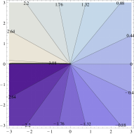
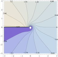
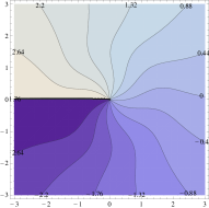
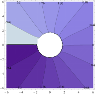
Figure 7: From left to right, lines of constant values of the Higgs phase for a) a NO vortex, b) a vortex computed in the limit of small $\beta$, where the backreaction of $\hat{A}_{r}$ onto the other fields can be neglected, c) a numerical solution with $\beta=0.40$ and $N=2$, and d) a numerical solution with $\beta=0.50$ displaying a ‘thick’ singularity. For the last two solutions we chose relatively large values of $\beta$ in order to make the effects of non-linearities more evident. Notice how non-linear effects associated with our derivative interactions qualitatively change the Higgs phase profile.

It is clear that for Galileon Higgs vortices the figure is not symmetric under a reflection around the $x_{1}$ axis. At sufficiently large values of the parameter $\beta$, the solution of the phase ceases to be well defined in the entire radial coordinate, and the vortex core is substituted by a ‘thick’ singularity (recall that we graphically met this phenomenon also in Fig 4 when discussing the profile for $\hat{A}_{r}$).

It is interesting to speculate what are the physical consequences of this fact. In particular what happens in the interior part of the thick singularity, that we define as the cylindrical surface with boundary at $r=r_{c}$ where the square root turns complex. Possibly, a solution with the same Ansatz (30) as the one we considered arises, but with different ‘vorticity’ (in the sense that while the exterior solution has asymptotically a vorticity (say) $N=1$, the interior solution satisfies boundary conditions at the origin that correspond to higher vorticity $N>1$). Such configuration would be well-behaved for $r\to 0$, and then would continuously connect with the exterior solution at the core surface $r_{c}$. However, in trying to explicit determine the solution, we numerically find that some of the field first derivatives are discontinuous at $r=r_{c}$.

Hence in these theories the system seems to need a sort of ‘thick brane’ regularization of a singularity. It might be that such systems are related to – and find applications for – the SLED proposal pushed forward by Burgess and collaborators (see e.g. Aghababaie:2003wz ), that makes use of the properties of codimension two object for addressing the cosmological constant problem. We leave these questions to further study.

3.6 The energy functional for the galileon vortex

It is a natural question to ask whether our configurations are stable under small perturbations. For the case of Abelian Higgs vortex, the energy functional is known to be bounded from below: a BPS bound exists corresponding to a minimum for the energy. For the case of Galileon vortex, a similar result does not hold: the existence of a BPS bound is not automatic, and additional assumptions on the configurations considered have to be imposed. On the other hand, our configurations are characterized by non-vanishing vorticity – a topologically conserved number – hence they cannot continuosly change and decay to zero vorticity configurations. Moreover, we are able to show that the energy density is bounded for the static solutions we considered in the previous section.

First, we discuss the issue of a BPS bound for a Galileon Higgs vortex. In section 2.3 we saw that when the BPS bound, $\lambda=2e^{2}$, and the self-dual equations (17) are satisfied, the energy functional for the Abelian-Higgs Lagrangian reaches the minimum

$$\mathcal{E}_{AH}=e\eta^{2}\left|\int d^{2}xB\right|.$$

We now analyze self-dual equations for the Abelian Higgs-Galileon Lagrangian (33). For this purpose, the first step is to write the Lagrangian for Galileon Higgs in terms of the derivative operators $D_{\pm}\equiv D_{1}\pm iD_{2}$, this gives

$$\mathcal{L}_{6} =\mathrm{Im}\left\{-\frac{1}{4}\left(|D_{+}\Phi|^{2}+|D_{-}\Phi|^{2}\right)\Phi^{\star}D^{2}\Phi\right.$$

$$\left.-\frac{1}{4}\left[(D_{+}\Phi)(D_{-}\Phi)^{\dagger}\Phi^{\star}D_{-}D_{-}\Phi+(D_{+}\Phi)^{\dagger}(D_{-}\Phi)\Phi^{\star}D_{+}D_{+}\Phi\right]\right\}.$$ (37)

In order to isolate the explicit dependence on the magnetic field, we use $D^{2}=D_{\mp}D_{\pm}\mp iBe$, which can be proved by expanding $(D_{1}\mp iD_{2})(D_{1}\pm iD_{2})$. It also follows that $2D^{2}=D_{-}D_{+}+D_{+}D_{-}$. Assuming that all the fields are static, the total energy functional is the negative of the spatial part of the total Lagrangian (33),

$$\mathcal{E}_{AHG} =\int d^{2}x\left[\frac{1}{2}\left(B\mp e(|\Phi|^{2}-\eta^{2})\right)^{2}+|D_{\pm}\Phi|^{2}+\left(\frac{\lambda}{4}-\frac{e^{2}}{2}\right)\left(|\Phi|^{2}-\eta^{2}\right)^{2}\mp e\eta^{2}B\right.$$

$$\left.\mp\frac{\beta}{4}\left(|D_{+}\Phi|^{2}+|D_{-}\Phi|^{2}\right)|\Phi|^{2}Be+\frac{\beta}{4}\left(|D_{+}\Phi|^{2}+|D_{-}\Phi|^{2}\right)\text{Im}[\Phi^{\star}D_{\mp}D_{\pm}\Phi]+\frac{\beta}{4}M_{ab}\right],$$ (38)

where we have defined

$$M_{ab}=\text{Im}\left[(D_{+}\Phi)(D_{-}\Phi)^{\dagger}\Phi^{\star}D_{-}D_{-}\Phi+(D_{+}\Phi)^{\dagger}(D_{-}\Phi)\Phi^{\star}D_{+}D_{+}\Phi\right]\,.$$ (39)

The candidate for a self-dual point of the AH and of the AHG models is the same: indeed the potential term of $\mathcal{E}_{AHG}$, which we identify by the coefficient $\lambda$, is cancelled at $\lambda=2e^{2}$. However, a relevant difference is that for the AHG model the energy functional at the self-dual point is not automatically bounded from below since the last two terms in (38) are not automatically positive definite. A sufficient (but by no means necessary) condition to have an energy functional bounded from below is

$$\frac{\beta}{4}\left(|D_{+}\Phi|^{2}+|D_{-}\Phi|^{2}\right)\text{Im}[\Phi^{\star}D_{\mp}D_{\pm}\Phi]+\frac{\beta}{4}M_{ab}\geq c\,,$$ (40)

for a certain constant $c$ which can be negative as long as the total energy remains positive. This is the simplest way we found to make sure that the Abelian Higgs-Galileon system has an energy density bounded from below —other possibility might exist though. Given these preliminary results, it would be interesting to study more in general the stability of our configurations under small fluctuations, and to explore alternative methods to obtain the BPS equations for Galileon vortices, such as methods based on the energy-momentum tensor deVega:1976mi or on the Lagrangian of the system rather than on the Hamiltonian Atmaja:2014fha .

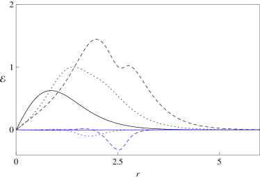
Figure 8: The total energy functional for $(\beta=0.1,N=1),(\beta=0.4,N=2)$ and $(\beta=0.5,N=3)$, is shown in solid, dotted and dashed lines respectively. The energy functional always develops a minimum at $r=0$. As $\beta$ increases, the energy density concentrates farther away from the origin and the total energy increases. In blue, we show the contribution from $\mathcal{L}_{6}$.

We end this section showing that the static configurations discussed in section 3.4 have positive definite energy for the values of $\beta$ we considered. We do not use the Lagrangian in terms of $D_{\pm}$, eq. (38), but rather we work directly with the static axially-symmetric ansatz. Then

$$\mathcal{E}_{AHG}[\hat{A}_{a}(r),X(r)]=-2\pi\int_{0}^{\infty}\left(\mathcal{L}_{AH}[\hat{A}_{a}(r),X(r)]+\mathcal{L}_{(6)}[\hat{A}_{a}(r),X(r)]\right)rdr.$$ (41)

The integrand of this expression is plotted in Fig. 8. The contribution to the energy coming from $\mathcal{L}_{(6)}$ is negligible only for $\beta=0.1$, and it is centred around the region where the non-linearities are relatively large, creating a local minimum. For any $\beta$ the energy of the vortex is finite and it always develops a global minimum at the locus of the vortex. If the non-linearities due to the derivative couplings are too large, we can suspect that the local minimum due to $\mathcal{L}_{6}$ approaches to zero, and if it tries to drive the total energy below zero then a thick singularity is formed. There might be well-behaved complete solutions where there are two global minima, both of them at $\mathcal{E}_{AHG}=0$, however we could not find numerically such solutions.

4 Coupling with gravity

It is known that a NO vortex coupled to gravity backreacts on the geometry, generating a space-time with a conical singularity when seen by a distant observer (see e.g. Gregory:1987gh ; Gregory:1997wk ). In this section we study the coupling to gravity of a Galileon Higgs vortex. We are interested to determine the gravitational backreaction of the field profiles of the vortex configuration that we determined in the previous sections. We will learn that, in a sense, Einstein equations ‘suggest’ a field dependent change of coordinates adapted to the vortex profile, that makes the resulting geometry particularly symmetric .

For our purpose, we consider the Einstein equations minimally coupled to the energy momentum tensors of the Abelian Higgs model and of the Higgs Galileon contributions. Despite we work in four spacetime dimensions we consider only the Galileons given by $\mathcal{L}^{(6)}$. In this way, we avoid the issue of having to include non-minimal couplings with gravity, that would be necessary to maintain a ghost-free condition Hull2 ; Tasinato:2014eka ; Heisenberg:2014rta .

The energy momentum tensor for the AH model is

$$T^{(AH)}_{{a}{b}} =\frac{2}{\sqrt{-g}}\frac{\delta(\sqrt{-g}\mathcal{L}_{AH})}{\delta g^{{a}{b}}}=-g_{{a}{b}}\mathcal{L}_{AH}+2\frac{\delta\mathcal{L}_{AH}}{\delta g^{{a}{b}}}$$

$$=-g_{{a}{b}}\mathcal{L}_{AH}+2\eta^{2}\nabla_{a}X\nabla_{b}X+2\eta^{2}X^{2}\hat{A}_{a}\hat{A}_{b}+\frac{1}{e^{2}}F_{{a}c}F^{c}{}_{b},$$ (42)

while for the Galileon Higgs we obtain

$$T^{(6)}_{{a}{b}}=-g_{{a}{b}}\mathcal{L}_{6}+2\beta\eta^{4}\left(L_{{a}{b}}Q+LQ_{{a}{b}}-Q_{{a}}{}^{c}{}L_{c{b}}-L_{{a}c}Q^{c}{}_{{b}}\right).$$ (43)

We restrict ourselves to small $\beta$ coupling, and to weak coupling to gravity. In particular we are interested in establishing how the spacetime metric can take into account the breaking of reflection symmetry shown by the Galileon Higgs vortex profiles. Inspection of the energy momentum tensor reveals that – for field configurations corresponding to a vortex – the profile for the gauge invariant field $\hat{A}_{r}$ induces a component $T^{(AH)}_{r\theta}$, which is not supported by the Einstein tensor relative to a diagonal metric. For this reason, we take a metric Ansatz of the form

$$ds^{2}=e^{2(\gamma-\Psi)}(dt^{2}-dr^{2})-e^{2\Psi}dz^{2}-\alpha^{2}e^{-2\Psi}d\theta^{2}-\beta\,\omega drd\theta,$$ (44)

where $\gamma$, $\Psi$, $\omega$ and $\alpha$ are functions only of $r$. The parameter $\beta$ – the same that multiplies $\mathcal{L}_{6}$ – is taken to be small. As we will see in a moment, such form of the metric, breaking the reflection symmetry $\theta\to-\theta$, is in principle able to accommodate for the specific field profiles we are considering. On the other hand, this metric is still axially symmetric, since all the metric components depend only on the radial direction. As we will discuss towards the end of this section, a coordinate transformation exists that is adapted to the vortex configuration, and that renders (44) explicitly diagonal.

4.1 Solving Einstein equations in a small $\beta$ limit

For the moment we work with the metric (44), to investigate how the non-diagonal metric component $\omega$ depends on the field profile. The Einstein equations controlling gravity minimally coupled to the vortex are

$$G_{ab}=8\pi G(T^{(AH)}_{ab}+T^{(6)}_{ab}).$$ (45)

Boost invariance along the $z$-axis is automatically satisfied for the energy-momentum tensor of the Abelian Higgs model (i.e. $T^{AH}{}^{t}\!{}_{t}=T^{AH}{}^{z}\!{}_{z}$), however it only holds for the Galileon Higgs if we impose the condition $\gamma=2\Psi$, which we will do from now on. As we explained, we take a small $\beta$ limit: the configuration of $\hat{A}_{r}$ can be easily obtained from eq (35) by expanding at first order in $\beta$:

$$\hat{A}_{r}\simeq\left(\frac{6\beta\eta^{2}X^{2}}{r}\right)\,\left[\frac{\hat{A}_{\theta}}{r^{2}}(\hat{A}_{\theta}-r\hat{A}_{\theta}^{\prime}{})+\frac{X^{\prime}}{3X}\left(\frac{X^{\prime}{}}{X}-\frac{4\hat{A}_{\theta}^{2}}{r}\right)\right]$$ (46)

and is then proportional to the quantity $\beta\eta^{2}$. In addition, in this limit $X$ and $\hat{A}_{\theta}$ describe standard NO vortices.

At our level of approximation – leading order in $\beta$ – the non-vanishing components of the total energy momentum tensor are only in the Abelian Higgs sector, and are given by:

$$T^{AH}_{tt} =\mathcal{P}_{t}=\frac{1}{4}e^{\gamma}\lambda\eta^{4}(X^{2}-1)^{2}+\frac{e^{2\gamma}\eta^{2}\hat{A}_{\theta}^{2}X^{2}}{\alpha^{2}}+\frac{e^{\gamma}\hat{A}_{\theta}^{\prime}{}^{2}}{2q^{2}\alpha^{2}}+\eta^{2}X^{\prime}{}^{2},$$ (47a)

$$T^{AH}_{rr} =\mathcal{P}_{r}=-\frac{1}{4}e^{\gamma}\lambda\eta^{4}(X^{2}-1)^{2}-\frac{e^{2\gamma}\eta^{2}\hat{A}_{\theta}^{2}X^{2}}{\alpha^{2}}+\frac{e^{\gamma}\hat{A}_{\theta}^{\prime}{}^{2}}{2q^{2}\alpha^{2}}+\eta^{2}X^{\prime}{}^{2},$$ (47b)

$$T^{AH}_{\theta\theta} =\mathcal{P}_{\theta}=-\frac{1}{4}e^{-\gamma}\lambda\eta^{4}\alpha^{2}(X^{2}-1)^{2}+\eta^{2}\hat{A}_{\theta}^{2}X^{2}+\frac{e^{-\gamma}\hat{A}_{\theta}^{\prime}{}^{2}}{2q^{2}}-e^{-2\gamma}\eta^{2}\alpha^{2}X^{\prime}{}^{2},$$ (47c)

$$T^{AH}_{zz} =-\mathcal{P}_{t}=-T^{AH}_{tt},$$ (47d)

$$T^{AH}_{r\theta} =\beta\mathcal{M}=\beta\frac{\eta^{2}\omega}{2}\left[\frac{4\eta^{2}\hat{A}_{r}^{(0)}\hat{A}_{\theta}X^{2}}{\omega}-\frac{1}{4}\eta^{2}\lambda(X^{2}-1)^{2}-\frac{e^{\gamma}\hat{A}_{\theta}^{2}X^{2}}{\alpha^{2}}+\frac{\hat{A}_{\theta}^{\prime}{}^{2}}{2q^{2}\alpha^{2}\eta^{2}}-e^{-\gamma}X^{\prime}{}^{2}\right].$$ (47e)

where we have defined $\hat{A}_{r}\equiv\beta\eta^{2}\hat{A}_{r}^{(0)}$. We emphasize that the fields $X$ and $\hat{A}_{\theta}$ have profiles corresponding to a NO vortex, since we are neglecting the ${\cal O}(\beta^{2})$ effects associated with the backreaction of $\hat{A}_{r}$ on their equations of motion.

Thus, the only consequence of the presence of $\mathcal{L}^{(6)}$ is that for Galileon Higgs vortices $\hat{A}_{r}$ is necessarily different from zero and therefore $T^{AH}_{r\theta}$ cannot be turned off. It is convenient to rescale $r\to\eta^{-1}r$ and $\alpha\to\eta^{-1}\alpha$, so that $\eta$ effectively controls the coupling strength between the vortex and the Einstein tensor,

$$\alpha^{\prime\prime} =-4\pi G\eta^{2}\alpha(\mathcal{P}_{0}-\mathcal{P}r),$$

$$(\alpha\gamma^{\prime})^{\prime} =4\pi G\eta^{2}\alpha(\mathcal{P}_{r}+\frac{e^{2\gamma}}{\alpha^{2}}\mathcal{P}_{\theta}),$$

$$\alpha^{\prime}\gamma^{\prime} =\frac{{\alpha}\gamma^{\prime}{}^{2}}{4}+4\pi G\eta^{2}{\alpha}\mathcal{P}_{r},$$

$$\frac{1}{8}e^{-\gamma}\omega(\gamma^{\prime}{}^{2}+4\gamma^{\prime\prime}) =4\pi G\eta^{2}\mathcal{M}.$$ (48)

Note that $\omega$ is completely determined by the solutions for the other fields, and it vanishes when $\hat{A}_{r}^{(0)}=0$ because its equation of motion acquires the form

$$\omega F(X,\hat{A}_{\theta},\alpha,\gamma,X^{\prime},\hat{A}_{\theta}^{\prime},\gamma^{\prime})=0,$$

where the function $F$ of the various fields does not generically vanish for vortex configurations. To the lowest order in $\eta^{2}$ and in the metric corrections, we find from the first, third, and fourth equations in (48) the solutions

$$\alpha =\left[1-4\pi G\eta^{2}\int r(\mathcal{P}_{0}-\mathcal{P}_{r})dr\right]r+4\pi G\eta^{2}\int r^{2}(\mathcal{P}_{0}-\mathcal{P}_{r})dr,$$ (49a)

$$\gamma =4\pi G\eta^{2}\int r\mathcal{P}_{r}dr,$$ (49b)

$$\omega =\frac{2\pi\mathcal{M}}{(r\mathcal{P}_{r})^{\prime}}.$$ (49c)

Using the Bianchi identity $r^{2}(r\mathcal{P}_{r})^{\prime}=\mathcal{P}_{\theta}+\mathcal{O}(\beta^{2})$ we can verify that the second equation in (48) is also satisfied by these solutions, and we can rewrite the solution for $\omega$ as $\omega\sim r^{2}\mathcal{M}/\mathcal{P}_{\theta}$.

The fields in the Galileon Higgs vortex decay fast, therefore the integrals in the solutions for the metric components quickly reach their asymptotic, constant values. To verify that $\omega$ is well behaved asymptotically we can consider the expression for $\hat{A}_{r}$ in the small $\beta$ limit, eq (46). Since $X(r\to\infty)\sim 1$ we see that $\hat{A}_{r}$ decays at least as $\hat{A}_{\theta}/r^{3}$. Using this information we learn that the first term in (47e) is sub-dominant with respect to the other terms, so that $\mathcal{M}/\mathcal{P}_{\theta}$ decays as $\omega/r^{2}$, and the only solution to eq. (49c) is $\omega=0$. This implies that for large $r$ the metric has the same form as the metric that would be obtained in the presence of a weakly coupled NO vortex, which was derived in Gregory:1987gh and corresponds to a conical metric with a deficit angle $\Delta=8\pi G\mu$ as seen by an asymptotic observer, where $\mu$ is the energy per unit length of the string.

With a little additional effort, we can also derive the asymptotic profiles for the fields involved, within our approximations. We start considering the asymptotic solutions for the profiles of $X$ and $\hat{A}_{\theta}$ for the NO vortex, also valid for our configuration, at leading order in a small $\beta$ expansion (see e.g. Rubakov:2002fi ):

$$X\approx 1-x_{0}\frac{e^{-\eta\sqrt{\lambda}r}}{\sqrt{r}},\ \ \ \hat{A}_{\theta}\approx a_{0}\sqrt{r}e^{-\sqrt{2}e\eta r},$$ (50)

where $x_{0}$, $a_{0}$, and $b_{0}$ (used in the next equation) are constants determined by the boundary conditions.

Plugging these solutions in (46) we get

$$\hat{A}_{r}\approx\frac{b_{0}}{r}{e^{-2\sqrt{2}e\eta r}},$$ (51)

Using these results and the background metric to evaluate $\mathcal{M}$ and $\mathcal{P}_{\theta}$ we find that asymptotically $\omega$ is given by

$$\omega\approx-\frac{1}{r^{3/2}}e^{-2\sqrt{2}er\eta}.$$ (52)

Hence we see that it has an exponential decay for large values of $r$.

4.2 A convenient coordinate transformation

So far, working at linearised order in $\beta$, we have shown that the field profile for $\hat{A}_{r}$ turn on a new metric component when coupling with gravity, that we denote with $\omega$ in eq (44). For concluding this Section, we show that taking advantage of the invariance under diffeomorphisms of General Relativity we can perform a change of coordinates that renders the metric diagonal and manifestly axially symmetric. Einstein equations relate the magnitude of the metric component $\omega$ – that breaks the reflection symmetry $\theta\to-\theta$ in metric (44) – with the size of the field $\hat{A}_{r}$, that as we learned is producing the twirling features of the vortex configurations. On the other hand, always working at leading order in $\beta$, the following redefinition of the angular coordinate

$${d\theta\,\to\,d\theta-\frac{\beta\,\omega}{2\,\alpha^{2}}\,e^{2\psi}\,dr}$$ (53)

renders the geometry manifestly axially symmetric, giving it a diagonal form. Such field redefinition adapts the geometry to the vortex configuration, and effectively ‘eats up’ the contribution of the field $\hat{A}_{r}$ that would cause an off-diagonal component $T_{r\theta}$ in the energy momentum tensor. Hence in this specific coordinate system, the coordinates adapt to the vortex lines, and the derivative interactions modulate the radial dependence of $\hat{A}_{\theta}$, $X$. It would be interesting to investigate whether the arguments we developed in this section can be extended to arbitrary values of $\beta$, to understand the gravitational backreaction in large $\beta$ regimes.

5 Outlook

In this work we presented and analysed finite energy vortex solutions in a 2+1 dimensional Abelian Higgs model supplemented by higher order derivative self-interactions for the Higgs field. Such interactions have been first introduced in Hull:2014bga for providing a Higgs mechanism to spontaneously break the gauge symmetry through vector Galileon interactions Tasinato:2014eka ; Heisenberg:2014rta . They are ghost free, and in a suitable high energy limit they enjoy Galilean symmetries that can help for protect their structure from quantum corrections. We dubbed this system Galileon Higgs. Within this framework, we have been able to determine vortex solutions characterised by topologically conserved winding numbers. They have features that make them qualitatively different from the Nielsen-Olesen vortex. The derivative non-linear interactions turn on new field profiles for gauge invariant field potentials that violate a reflection symmetry around one of the axis of the Cartesian coordinates, and lead to regular configurations that necessarily also break the axial symmetry of the configuration. Interestingly, some of the equations of motion reduce to quadratic algebraic equations, simplifying considerably our analysis. Moreover, we have also promoted our 2+1 dimensional solution to a 3+1 dimensional one, and coupled the resulting system to gravity, showing that gravity backreaction leads to a space-time that, depending on the coordinates one choose, can be described by a metric without reflection invariance, or a metric with non-standard angular and radial coordinates. One way or another, the effect of having a vortex with non-trivial field profiles is seen as a contribution to the space-time curvature and deficit angle.

Our results can find several applications and suggest further lines of research, opening possibilities for finding new classes of vortex solutions in system with derivative self-interactions. For example:

• It would be interesting to find non-relativistic analogues of our Galileon Higgs vortex configurations, for example in the context of superfluids or superconductors. Such non-standard vortex configurations might play some role in cases in which derivative interactions are important in the pattern of symmetry breaking. Also, in this context, the dynamics of multi-vortex solutions would be interesting to investigate, since it can be important when discussing the stability of our configurations when considering values of the vorticity larger than one.

• As discussed in the introduction, one motivation for studying cosmic strings/vortex solutions in this context is to understand screening mechanisms – as Vainshtein mechanism – in absence of spherical symmetry, taking into account the backreaction of all fields including gravity. This can be important when testing screening mechanisms in the context of cosmology as for understanding the cosmic web structure, where filaments and voids form (see e.g. Falck:2014jwa ; Falck:2015rsa ). Our results suggest that in some cases – depending on the field content and their interactions – the gravitational backreaction can be rather subtle, and axial symmetry of the system can be not manifest even for cylindrical sources. These findings might offer indications for determining accurate semi-analytical models for structure formation in models with screening mechanisms.

We plan to develop these arguments in further studies.

- (1) A. A. Abrikosov, “The magnetic properties of superconducting alloys,” JPCS 2 (1957) 3
- (2) H. B. Nielsen and P. Olesen, “Vortex Line Models for Dual Strings,” Nucl. Phys. B 61 (1973) 45.
- (3) R. J. Donnelly, “Quantized Vortices and Turbulence in Helium II,” Annual Review of Fluid Mechanics, Vol. 25: 325-371
- (4) A. Vilenkin and E. P. S. Shellard, “Cosmic Strings and Other Topological Defects,”
- (5) E. J. Weinberg, “Classical solutions in quantum field theory : Solitons and Instantons in High Energy Physics,”
- (6) G. V. Dunne, “Aspects of Chern-Simons theory,” hep-th/9902115.
- (7) M. Hull, K. Koyama and G. Tasinato, “A Higgs Mechanism for Vector Galileons,” arXiv:1408.6871 [hep-th].
- (8) A. Nicolis, R. Rattazzi and E. Trincherini, “The Galileon as a local modification of gravity,” Phys. Rev. D 79 (2009) 064036 [arXiv:0811.2197 [hep-th]].
- (9) A. Nicolis and R. Rattazzi, “Classical and quantum consistency of the DGP model,” JHEP 0406 (2004) 059 [hep-th/0404159].
- (10) P. Brax, “Screening mechanisms in modified gravity,” Class. Quant. Grav. 30 (2013) 214005.
- (11) E. Babichev and C. Deffayet, “An introduction to the Vainshtein mechanism,” Class. Quant. Grav. 30 (2013) 184001 [arXiv:1304.7240 [gr-qc]].
- (12) E. Babichev and G. Esposito-Farèse, “Time-Dependent Spherically Symmetric Covariant Galileons,” Phys. Rev. D 87 (2013) 044032 [arXiv:1212.1394 [gr-qc]].
- (13) F. Sbisa, G. Niz, K. Koyama and G. Tasinato, “Characterising Vainshtein Solutions in Massive Gravity,” Phys. Rev. D 86 (2012) 024033 [arXiv:1204.1193 [hep-th]].
- (14) K. Koyama, G. Niz and G. Tasinato, “Effective theory for the Vainshtein mechanism from the Horndeski action,” Phys. Rev. D 88 (2013) 021502 [arXiv:1305.0279 [hep-th]].
- (15) J. K. Bloomfield, C. Burrage and A. C. Davis, “The Shape Dependence of Vainshtein Screening,” arXiv:1408.4759 [gr-qc].
- (16) J. Chagoya, K. Koyama, G. Niz and G. Tasinato, “Galileons and strong gravity,” JCAP 1410 (2014) 10, 055 [arXiv:1407.7744 [hep-th]].
- (17) S. Endlich, K. Hinterbichler, L. Hui, A. Nicolis and J. Wang, “Derrick’s theorem beyond a potential,” JHEP 1105 (2011) 073 [arXiv:1002.4873 [hep-th]].
- (18) A. Padilla, P. M. Saffin and S. Y. Zhou, “Multi-galileons, solitons and Derrick’s theorem,” Phys. Rev. D 83 (2011) 045009 [arXiv:1008.0745 [hep-th]].
- (19) G. H. Derrick, “Comments on nonlinear wave equations as models for elementary particles,” J. Math. Phys. 5 (1964) 1252.
- (20) G. Tasinato, “Cosmic Acceleration from Abelian Symmetry Breaking,” JHEP 1404 (2014) 067 [arXiv:1402.6450 [hep-th]].
- (21) L. Heisenberg, “Generalization of the Proca Action,” JCAP 1405 (2014) 015 [arXiv:1402.7026 [hep-th]].
- (22) K. Kamada, T. Kobayashi, M. Yamaguchi and J. Yokoyama, “Higgs G-inflation,” Phys. Rev. D 83 (2011) 083515 [arXiv:1012.4238 [astro-ph.CO]]; K. Kamada, T. Kobayashi, T. Takahashi, M. Yamaguchi and J. Yokoyama, “Generalized Higgs inflation,” Phys. Rev. D 86 (2012) 023504 [arXiv:1203.4059 [hep-ph]].
- (23) M. Lake and J. Ward, “A Generalisation of the Nielsen-Olesen Vortex: Non-cylindrical strings in a modified Abelian-Higgs model,” JHEP 1104 (2011) 048 [arXiv:1009.2104 [hep-ph]].
- (24) T. Kawabe and S. Ohta, “Chaos and stability of Nielsen-Olesen vortex solution with cylindrical symmetry at critical coupling,” Phys. Lett. B 392 (1997) 433.
- (25) D. P. Jatkar, G. Mandal and S. R. Wadia, “Nielsen-Olesen vortices in noncommutative Abelian Higgs model,” JHEP 0009 (2000) 018 [hep-th/0007078].
- (26) E. B. Bogomolny, “Stability of Classical Solutions,” Sov. J. Nucl. Phys. 24 (1976) 449 [Yad. Fiz. 24 (1976) 861].
- (27) M. K. Prasad and C. M. Sommerfield, “An Exact Classical Solution for the ’t Hooft Monopole and the Julia-Zee Dyon,” Phys. Rev. Lett. 35 (1975) 760.
- (28) S. R. Coleman, S. J. Parke, A. Neveu and C. M. Sommerfield, “Can One Dent a Dyon?,” Phys. Rev. D 15 (1977) 544.
- (29) T. Clifton, P. G. Ferreira, A. Padilla and C. Skordis, “Modified Gravity and Cosmology,” Phys. Rept. 513 (2012) 1 [arXiv:1106.2476 [astro-ph.CO]].
- (30) G. Tasinato, “A small cosmological constant from Abelian symmetry breaking,” Class. Quant. Grav. 31 (2014) 225004 [arXiv:1404.4883 [hep-th]].
- (31) Y. Aghababaie, C. P. Burgess, S. L. Parameswaran and F. Quevedo, “Towards a naturally small cosmological constant from branes in 6-D supergravity,” Nucl. Phys. B 680 (2004) 389 [hep-th/0304256]; Y. Aghababaie et al., “Warped brane worlds in six-dimensional supergravity,” JHEP 0309 (2003) 037 [hep-th/0308064]. C. P. Burgess, F. Quevedo, G. Tasinato and I. Zavala, “General axisymmetric solutions and self-tuning in 6D chiral gauged supergravity,” JHEP 0411 (2004) 069 [hep-th/0408109].
- (32) H. J. de Vega and F. A. Schaposnik, Phys. Rev. D 14 (1976) 1100. doi:10.1103/PhysRevD.14.1100
- (33) A. N. Atmaja and H. S. Ramadhan, Phys. Rev. D 90, no. 10, 105009 (2014) doi:10.1103/PhysRevD.90.105009 [arXiv:1406.6180 [hep-th]].
- (34) R. Gregory, “Gravitational Stability of Local Strings,” Phys. Rev. Lett. 59 (1987) 740.
- (35) R. Gregory and C. Santos, “Cosmic strings in dilaton gravity,” Phys. Rev. D 56 (1997) 1194 [gr-qc/9701014].
- (36) M. Hull, K. Koyama and G. Tasinato, “Covariantised Vector Galileons,” arXiv:1510.07029 [hep-th].
- (37) V. A. Rubakov, “Classical theory of gauge fields,” Princeton, USA: Univ. Pr. (2002) 444 p
- (38) B. Falck, K. Koyama, G. b. Zhao and B. Li, “The Vainshtein Mechanism in the Cosmic Web,” JCAP 1407 (2014) 058 [arXiv:1404.2206 [astro-ph.CO]].
- (39) B. Falck, K. Koyama and G. B. Zhao, “Cosmic Web and Environmental Dependence of Screening: Vainshtein vs. Chameleon,” JCAP 1507 (2015) 07, 049 [arXiv:1503.06673 [astro-ph.CO]].