Massive star formation by accretion

Abstract

Context. Massive stars likely form by accretion and the evolutionary track of an accreting forming star corresponds to what is called the birthline in the HR diagram. The shape of this birthline is quite sensitive to the evolution of the entropy in the accreting star.

Aims. We first study the reasons why some birthlines published in past years present different behaviours for a given accretion rate. We then revisit the question of the accretion rate, which allows us to understand the distribution of the observed pre-main-sequence (pre-MS) stars in the Hertzsprung-Russell (HR) diagram. Finally, we identify the conditions needed to obtain a large inflation of the star along its pre-MS evolution that may push the birthline towards the Hayashi line in the upper part of the HR diagram.

Methods. We present new pre-MS models including accretion at various rates and for different initial structures of the accreting core. We compare them with previously published equivalent models. From the observed upper envelope of pre-MS stars in the HR diagram, we deduce the accretion law that best matches the accretion history of most of the intermediate-mass stars.

Results. In the numerical computation of the time derivative of the entropy, some treatment leads to an artificial loss of entropy and thus reduces the inflation that the accreting star undergoes along the birthline. In the case of cold disc accretion, the existence of a significant swelling during the accretion phase, which leads to radii $\gtrsim 100\,R_{\odot}$ and brings the star back to the red part of the HR diagram, depends sensitively on the initial conditions. For an accretion rate of $10^{-3}\,M_{\odot}\rm\,yr^{-1}$, only models starting from a core with a significant radiative region evolve back to the red part of the HR diagram. We also obtain that, in order to reproduce the observed upper envelope of pre-MS stars in the HR diagram with an accretion law deduced from the observed mass outflows in ultra-compact HII regions, the fraction of the mass that is accreted onto the star should represent a decreasing fraction of the mass outflows when the mass of the accreting object increases. In other words, the accretion efficiency (mass effectively accreted onto the star with respect to the total in falling matter) decreases when the mass of the star increases.

1 Introduction

Massive stars are rare, but their influence on our Universe is critical. They give the main chemical and dynamical inputs to the interstellar medium. Most of the heavy elements in our Universe were produced in the core of massive stars or during their deaths. The mass-loss during their lifetimes, and more dramatically their deaths in supernovae, feed the interstellar medium with these newly produced heavy elements. Such outflows and explosions, as well as the stellar radiation itself, are also thought to be the main mechanisms that trigger star formation. Thus, massive stars drive the star formation in their host galaxies and make them evolve. However, the formation of massive stars is currently the most poorly known part of their evolution.

Stars form in the gravitational collapse of cold dense clouds. Since the collapse is highly non-homologous, hydrostatic equilibrium is first reached by a small central core while the rest of the cloud is still collapsing, nearly in free-fall (e.g. McNally 1964, Bodenheimer & Sweigart 1968, Larson 1969, 1972). As the collapse proceeds, the hydrostatic core evolves as a pre-main-sequence (pre-MS) star, with a mass increasing with time. This is the accretion scenario (e.g. Shu 1977, Stahler et al. 1980a, b, 1986b, 1986a, Palla & Stahler 1990, 1991, 1992).

In the case of spherical symmetry, it has been shown that this scenario is not valid for massive stars ($M\gtrsim 40\,M_{\odot}$) owing to their strong radiation field (Kahn 1974; Yorke & Kruegel 1977; Wolfire & Cassinelli 1987). But we know now that an accretion flow with a disc geometry allows this limitation to be circumvented (Nakano 1989; Yorke & Sonnhalter 2002; Krumholz et al. 2009; Peters et al. 2010; Kuiper et al. 2010, 2011). Hydrodynamic simulations for the accretion flow in massive proto-stellar clouds (e.g. Peters et al. 2010; Kuiper et al. 2010), as well as observations of high-mass protostellar objects (e.g. Fazal et al. 2008), suggest that the typical value of the accretion rate during the formation of massive stars is $\sim 10^{-3}\,M_{\odot}\rm\,yr^{-1}$. This is in contrast with the case of low-mass stars, for which values of $\sim 10^{-5}\,M_{\odot}\rm\,yr^{-1}$ are expected (see e.g. Stahler et al. 1980a, b; Stahler 1983).

The accretion scenario for massive star formation has been explored by many authors in a stellar evolution approach. Bernasconi & Maeder (1996), Norberg & Maeder (2000), Behrend & Maeder (2001), and Haemmerlé et al. (2013) have computed stellar models with accretion using the Geneva Stellar Evolution code. The accretion rates used in these works were increasing functions of time, i.e. of the actual stellar mass. In the low-mass range ($M\lesssim 2\,M_{\odot}$) values around $10^{-5}\,M_{\odot}\rm\,yr^{-1}$ were considered, while in the high-mass range ($M\gtrsim 10\,M_{\odot}$) the values were $\sim 10^{-3}\,M_{\odot}\rm\,yr^{-1}$.

Hosokawa & Omukai (2009) and Hosokawa et al. (2010) have also computed stellar models with accretion for the formation of massive stars, using their own code. The accretion rates they used were constant in time (i.e. independent of the actual stellar mass), and so already had high values ($\sim 10^{-3}\,M_{\odot}\rm\,yr^{-1}$) in the low-mass range. They found that when a star accretes at such high rates in the intermediate-mass range ($2\,M_{\odot}\lesssim M\lesssim 10\,M_{\odot}$), it goes through a rapid swelling phase where the stellar radius can increase by more than one order of magnitude, leading to values as high as several $100\,R_{\odot}$ depending on the physical conditions. They also found that above a critical accretion rate of $\simeq 2-3\times 10^{-3}\,M_{\odot}\rm\,yr^{-1}$, a second swelling occurs before the star can contract to the zero-age-main-sequence (ZAMS), leading to stellar radii near $1000\,R_{\odot}$. In this case, at a mass around $\sim 50\,M_{\odot}$, steady accretion is no longer possible owing to the high radiation pressure that approaches the Eddington limit.

Since the works listed above were published, the treatment of accretion in the Geneva Stellar Evolution code has been improved (Haemmerlé 2014). In the original version of the code, an inconsistency in the treatment of the time derivatives was responsible for an artificial loss of entropy during the accretion phase. This inconsistency has been removed in the new version of the code. In the present paper, we show how these improvements modify pre-MS evolution with accretion. The paper is organized as follows. In Sect. 2, we describe the improvements brought to the code. In Sect. 3, we present models computed with the new version of the code using constant accretion rates, and we compare the results with those obtained with the original version of the code and with those of other authors. In Sect. 4, we do the same with the time-dependent accretion rate used by Behrend & Maeder (2001) and Haemmerlé et al. (2013). The conclusions are summarized in Sect. 5.

2 Improvements in the code

A full description of the original treatment of accretion in the Geneva Stellar Evolution code has already been given in the previous papers (Bernasconi & Maeder 1996; Haemmerlé et al. 2013). Here we focus on the improvements implemented since the last paper. A full description of the treatment of accretion in the new version of the code is available in Haemmerlé (2014). The treatment for the burning of light elements is also described in Haemmerlé et al. (2013), and a general description of the other physical ingredients in the code is available in Eggenberger et al. (2008).

The new improvements are related to the time variation of the thermodynamic quantities. Among the four equations of structure, the equation of energy conservation is the only one that involves time, so this is the equation that makes the star evolve. The equation is obtained from the energetic balance of a given mass element $dm$. A fraction of the energy generated by nuclear reactions is transformed into heat, the rest is radiated,

$$\int\epsilon_{n}\,dm\,=\int{dq\over dt}\,dm+\int{\nabla\@vec{F}\over\rho}dm,$$ (1)

where $\epsilon_{n}$ is the energy generation rate by nuclear reactions, $q$ the heat by unit of mass, $t$ the time, $\@vec{F}$ the flux, and $\rho$ the mass density. Since this equality is satisfied for any mass element, we have

$$\epsilon_{n}={dq\over dt}+{\nabla\@vec{F}\over\rho}=T\,{ds\over dt}+{dL_{r}\over dM_{r}},$$ (2)

where $s$ is the specific entropy, $T$ the temperature, $L_{r}$ the luminosity in the shell of radius $r$, and $M_{r}$ the total mass contained in the interior of this shell. We emphasize that

$${d\over dt}=\left.{d\over dt}\right|_{M_{r}}$$ (3)

since we started from the energetic balance of a given mass element (Lagrangian coordinates).

An alternative treatment is to use the relative mass coordinate

$$\mu={M_{r}\over M},$$ (4)

which is not a Lagrangian coordinate in the case of accretion since $M$ increases with time. With this coordinate, Eq. (2) becomes

$$\epsilon_{n}=T\left.{ds\over dt}\right|_{\mu}-{\mu\dot{M}\over M}\cdot T{ds\over d\mu}+{1\over M}{dL_{r}\over d\mu}.$$ (5)

Equation. (5) contains one more term than Eq. (2), which is proportional to the accretion rate and the entropy gradient. Since the entropy increases outwards and $\dot{M}>0$ during accretion, this additional term is negative. This procedure has been used by e.g. Stahler et al. (1980a, b) and Hosokawa & Omukai (2009). These two methods are physically equivalent.

In our code, we keep the Lagrangian formulation using Eq. (2). However, in the original version, we treated the differential $ds$ as a time variation at fixed $\mu$ instead of fixed $M_{r}$. In the constant mass case, such a treatment is fully consistent since a fixed $\mu$ also corresponds to a fixed $M_{r}$. However, in the case of accretion, it leads to an artificial loss of entropy. This inconsistency is physically equivalent to the neglect of the additional term in Eq. (5). If we neglect this negative term, this is equivalent to assuming that $\left.{ds\over dt}\right|_{M_{r}}=\left.{ds\over dt}\right|_{\mu}$, while actually $\left.{ds\over dt}\right|_{M_{r}}=\left.{ds\over dt}\right|_{\mu}-{\mu\dot{M}\over M}\cdot T{ds\over d\mu}$. Thus, we see that the neglect of the additional term implies a value for the time derivative of the entropy that is too large or in other words, an artificial loss of entropy. This inconsistency has been removed in the new version of the code: we still use Eq. (2), but the differential $ds$ that appears in this equation is now treated consistently as a time variation at constant $M_{r}$.

For the accretion of entropy (i.e. the computation of $ds/dt$ in the layer newly accreted at each time step), we make the assumption that the entropy of the material that is accreted is the same as the entropy of the stellar surface before the material is accreted. This is the assumption of cold disc accretion (see e.g. Palla & Stahler 1992; Hosokawa et al. 2010; Haemmerlé et al. 2013). It corresponds to the case of an accretion flow with a thin disc geometry, allowing any entropy excess to be radiated away in the polar directions before it is advected in the stellar interior. Thus, we do not add any contribution from the gravitational energy liberated by the material when it is accreted, and the entropy profiles are built continuously. This assumption is generally considered as the lower limit for the accretion of entropy (e.g. Hosokawa et al. 2010). The corresponding boundary conditions are the usual photospheric boundary conditions.

We use the Schwarzschild criterion for convection without overshooting. The chemical composition is solar ($Z=0.014$) with the abundances of Asplund et al. (2005) and Cunha et al. (2006). For deuterium, we take a mass fraction of $5\times 10^{-5}$ as in Bernasconi & Maeder (1996), Norberg & Maeder (2000), Behrend & Maeder (2001), and Haemmerlé et al. (2013).

3 Models with constant accretion rates

3.1 Case with $\dot{M}=10^{-4}\,M_{\odot}\rm\,yr^{-1}$

In order to illustrate the effect of the improvements described in Sect. 2, we first consider a pre-MS star accreting at a constant rate of

$$\dot{M}=10^{-4}\,M_{\odot}\rm\,yr^{-1}$$ (6)

For the initial model, we consider

$$M=0.7\,M_{\odot}\qquad L=9.57\,L_{\odot}\qquad T_{\rm eff}=4130\,K$$ (7)

This initial model has a radius of $6.06\,R_{\odot}$ and is fully convective. Starting from this initial model, we compute two models accreting at the rate of Eq. (6), one with the original version of the code, the other with the new version, including the improvements described in Sect. 2. The evolutionary tracks and the evolution of the radii and the internal structures of both models are shown in Figs. 1 and 2.

Figure 1: Evolutionary tracks of two models having the same initial conditions (Eq. 7) accreting at the same rate ($10^{-4}\,M_{\odot}\rm\,yr^{-1}$), but computed with the two different versions of the code. The black dotted straight lines are iso-radius for the indicated values of $R$, and the black short-dashed line is the ZAMS of Ekström et al. (2012) with a few masses indicated. From bottom to top, the filled squares on each track are the apparition of the radiative core, the end of the convective envelope, and the apparition of the convective core (see Fig. 2).

Figure 2: Evolution of the stellar radius and the internal structure for the same models as in Fig. 1. The horizontal axis corresponds to the stellar mass, which is a time coordinate in the case of accretion. In each case, the upper line indicates the stellar radius, the other continuous and long-dashed lines indicate the boundary between radiation and convection. The thin blue dotted lines are iso-mass of 1, 2, 3, …, $21\,M_{\odot}$ for the model computed with the new version of the code.

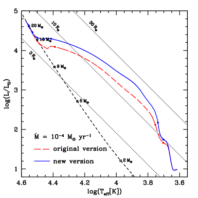
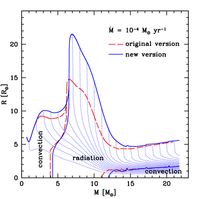
In the first stages of the evolution (low-mass range, $M\lesssim 2\,M_{\odot}$), both models are identical. In convective regions, the entropy gradient is flat, so that the time variation of entropy at fixed $\mu$ or at fixed $M_{r}$ is the same.

The initial value of the central temperature is too low for a significant D-burning, and the star takes its energy from gravitational contraction. At $M\simeq 1\,M_{\odot}$, the central temperature reaches $\sim 10^{6}K$ and D-burning becomes significant. Owing to its high sensitivity in temperature ($\epsilon_{\rm D}\sim T^{11.7}$, see e.g. Maeder 2009), D-burning has a thermostatic effect, leading to a central temperature $T_{c}$ that is nearly constant until the end of central burning. Since $T_{c}\sim M/R$, it produces an increase in the stellar radius, nearly linearly with respect to the stellar mass (see Fig. 2). The deuterium mass fraction decreases in the whole star, and goes to 0 at $M\simeq 2-3\,M_{\odot}$. D-burning becomes too weak for the star and gravitational contraction starts again.

It is at this point that both models start to diverge with a smaller radius for the original model than for the new model. But while the star is still fully convective, the differences remain relatively modest. The small differences that appear are due to the non-adiabaticity of convection in the external regions.

Since central D-burning is now negligible, $T_{c}$ can increase again, and the opacity decreases. At $M\simeq 4\,M_{\odot}$, a radiative core appears, earlier in the original model ($M=3.8\,M_{\odot}$) than in the new model ($M=4.3\,M_{\odot}$). The huge decrease in opacity in the deep regions leads to the so-called luminosity wave (e.g. Larson 1972; Hosokawa et al. 2010): the low opacity in the radiative core imposes a flux that is too strong for the convective envelope, in which opacity is still high. The convective envelope absorbs the flux, so that the luminosity profile has a maximum near the boundary between these two regions. As the temperature increases in the star, the radiative core grows in mass and the maximum in luminosity moves outwards. The energy absorbed by the convective envelope leads to an increase in the stellar radius, which becomes particularly strong as the convective envelope recedes.

It is at this point that the differences between the two models become really significant. While the original model reaches only $14.7\,R_{\odot}$, the new one reaches $21.5\,R_{\odot}$, which is 46% higher. Because of the strong entropy gradient that develops in the radiative regions, a $ds$ at a given $\mu$ or at a given $M_{r}$ are significantly different.

When the whole star becomes radiative, the radius decreases again, and the star contracts towards the ZAMS. Around $11-12\,M_{\odot}$, the triggering of the CN cycle produces a convective core, and the energy released by the nuclear reactions replaces the gravitational contraction as the main energy source of the star. Contraction slows down until the stellar radius reaches a minimum, which can be seen as the ZAMS at masses of $13.6\,M_{\odot}$ and $15.6\,M_{\odot}$ for the original and the new model, respectively. At this point, the differences between the two models become small again: for the original model the minimum radius is $4.3\,R_{\odot}$, while it is $4.7\,R_{\odot}$ for the new model (only 9% higher). Then, as accretion goes on the stellar radius increases nearly linearly with the stellar mass, following the ZAMS (see Fig. 1). We stopped the computation when the central mass fraction of hydrogen decreased by 0.3% with respect to its initial value.

To summarize, the differences between the two models are as follows:

• the new model evolves more slowly than the original;

• the new model reaches higher radii than the original, mainly during the swelling phase.

The other differences remain modest.

Why does the neglect of the additional term have the strongest effect during the swelling? Because the swelling occurs in the intermediate-mass range, when the star is fully radiative, having thus a strong entropy gradient. In this case, the artificial loss of entropy in the original model becomes significant. Using the homology relations $P\sim M^{2}/R^{4}$ and $T\sim M/R$ the specific entropy reads

$$s\sim-\ln{P\over T^{5/2}}\sim\ln(MR^{3})$$ (8)

(Hosokawa & Omukai 2009). It follows that, for a given mass, the smaller the entropy is, the smaller the radius. As a consequence, the artificial loss of entropy leads to artificially small radii, softening the swelling. Furthermore, since the gravitational contraction – which governs pre-MS evolution – corresponds to a decrease of the entropy, the artificial loss of entropy accelerates pre-MS evolution.

3.2 Case with $\dot{M}=10^{-3}\,M_{\odot}\rm\,yr^{-1}$

The typical value of the accretion rate for massive star formation is higher than the $10^{-4}\,M_{\odot}\rm\,yr^{-1}$ considered in Sect. 3.1. In the present section, we make the same comparison as in Sect. 3.1, but using the rate

$$\dot{M}=10^{-3}\,M_{\odot}\rm\,yr^{-1}.$$ (9)

For the initial model, we first consider

$$M=1.0\,M_{\odot}\qquad L=37.9\,L_{\odot}\qquad T_{\rm eff}=4130\,K$$ (10)

labelled CV1, which has a radius of $R=12.1\,R_{\odot}$ and is again fully convective. The evolutionary tracks and the evolution of the radii and the internal structures of models starting from CV1 accreting at the rate of Eq. (9) computed with both versions of the code are shown in Figs. 3 and 4.

Figure 3: Same as Fig. 1, but for an accretion rate of $10^{-3}\,M_{\odot}\rm\,yr^{-1}$ and the initial model CV1.

Figure 4: Same as Fig. 2, but for an accretion rate of $10^{-3}\,M_{\odot}\rm\,yr^{-1}$ and the initial model CV1. (The internal structure is shown only for the new model.)

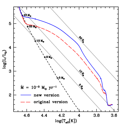
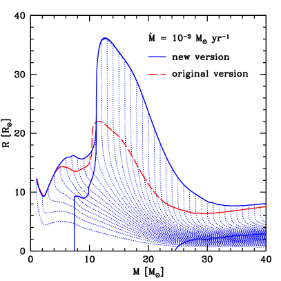
The result is qualitatively similar to the case with $10^{-4}\,M_{\odot}\rm\,yr^{-1}$. The original and the new model are identical until the end of central D-burning. Then the new model has larger radii and evolves more slowly than the original model. Again, the main difference is the magnitude of the swelling: while the maximum value of the stellar radius is $22.0\,R_{\odot}$ for the original model, it is $36.2\,R_{\odot}$ for the new model, which makes a relative difference of 65%. It illustrates the fact that the artificial loss of entropy is more important when the accretion rate is higher. For a given time-step $dt$ and a given value of $\mu$, the difference in $M_{r}$ between the model of age $t$ and the model of age $t+dt$ increases with the accretion rate since

$$dM_{r}=\mu\,dM=\mu\,\dot{M}dt.$$ (11)

In order to test the dependence of our results on the initial model, we compute two additional models with the new version of the code at the same rate of $10^{-3}\,M_{\odot}\rm\,yr^{-1}$, but using two different initial models, labelled CV2 and RC.

The CV2 model is given by

$$M=2.0\,M_{\odot}\qquad L=123\,L_{\odot}\qquad T_{\rm eff}=4270\,K.$$ (12)

This model has a radius of $20.4\,R_{\odot}$ and is fully convective, as is CV1. Both models are fully convective; CV2 differs from CV1 only in terms of global properties, and not in terms of internal structure. We note, however, that the CV2 model has a larger radius than the model of the same mass obtained by accretion starting from CV1. With CV1, the stellar radius reached when the mass is equal to $2\,M_{\odot}$ is only $9.4\,R_{\odot}$, so about a factor of two smaller than the radius of CV2. In agreement with Eq. (8), the larger radius of the CV2 model corresponds to a higher total amount of entropy.

Finally, the RC model is given by

$$M=2.0\,M_{\odot}\qquad L=4.32\,L_{\odot}\qquad T_{\rm eff}=5230\,K.$$ (13)

It has a radius of $2.53\,R_{\odot}$ and is thus much more compact than CV1 and CV2. Moreover, in contrast to all the previous cases, the initial RC model is not fully convective, but is made of a radiative core ($M_{r}<1.53\,M_{\odot}$) and a convective envelope. We note that for both CV2 and RC, we used a mass of $2\,M_{\odot}$, which is higher than for CV1. Because of numerical difficulties, it is easier to compute accreting models with the structure of RC at $M=2\,M_{\odot}$ than at $M=1\,M_{\odot}$. In order to allow a direct comparison, we used the same mass for CV2.

In terms of thermodynamic quantities, the main difference between the initial models CV2 and RC is the entropy profile. Both entropy profiles are shown in Fig. 5. First, we see that the global entropy is lower in the RC case than in the CV2 case, which was expected from Eq. (8). Moreover, in contrast to the entropy profile of CV2, which is flat (corresponding to a fully convective structure with adiabatic convection), the entropy profile of RC increases outwards (except in the convective envelope where it is flat). In the radiative core, the entropy profile increases nearly linearly with the Lagrangian coordinate with a gradient given by

$$\left.{ds\over dM_{r}}\right|_{\rm rad}\simeq 1.3\ k_{B}\,m_{H}^{-1}\,M_{\odot}^{-1}.$$ (14)

In other words, the RC model differs from the CV2 model not only in terms of global properties, but also (and more importantly) in terms of internal structure.

Figure 5: Entropy profiles of the initial models CV2 and RC. The square along the RC profile indicates the boundary between the radiative core and the convective envelope.

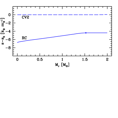
Another difference between these initial models is the deuterium abundance. The low central entropy of the RC model also corresponds to a high central temperature, which exceeds the temperature for D-burning: $T_{c}=6.1\times 10^{6}\,K$, instead of $7.7\times 10^{5}\,K$ in the case CV2. Indeed, Eq. (8) and $T_{c}\sim M/R$ give $s\sim\ln(M^{4}/T_{c}^{3})$, so that for a given mass, the lower is the entropy, the higher is the central temperature. With such a high temperature, we expect all the deuterium contained originally in the material of this “initial” model to be destroyed in the previous stages of the evolution, and we take $X_{2}=0$ in the initial model RC. However, we keep the usual mass fraction ($X_{2}=5\times 10^{-5}$, Sect. 2) in the accreted material, as in the CV cases.

Figure 6: Evolutionary tracks of the models computed from the initial models CV1, CV2 and RC at $\dot{M}=10^{-3}\,M_{\odot}\rm\,yr^{-1}$, using the new version of the code. For comparison, a series of points from the model MD3-D of Hosokawa et al. (2010) is indicated with connected black squares. The black dashed curve is the ZAMS of Ekström et al. (2012) with a few masses indicated, and the black dotted straight lines are iso-radius of 1, 10, 100 and $1000\,R_{\odot}$. The blue squares along the tracks correspond to the same masses as those indicated along the ZAMS. (Notice that, on the vertical axis, $L$ is the intrinsic stellar luminosity, without any contribution from the accretion luminosity.)

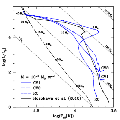
The evolutionary tracks obtained from these two new initial models are shown in Fig. 6, together with the track obtained from CV1 (which is the same as the blue track in Fig. 3). The evolution obtained from CV2 is similar to the CV1 case. The star is initially fully convective, until a radiative core appears, here at a mass of $8.8\,M_{\odot}$. Then the convective envelope recedes and disappears, while the luminosity wave described in Sect. 3.1 produces the swelling of the star. The radius reaches its maximum value of $48.6\,R_{\odot}$ at a mass of $12.6\,M_{\odot}$, before the star contracts towards the ZAMS (reached at $M\sim 30\,M_{\odot}$). This example shows that a change in the total amount of entropy in the initial model, without any difference in the internal distribution of the entropy, does not result in a significant difference in the stellar evolution during the accretion phase. For instance, while the initial radius of the CV2 model is more than a factor of 2 larger than that of CV1, the maximum value reached by the radius during the swelling is increased by only 34%.

The evolution corresponding to the RC model shows significant differences compared to the CV cases (i.e. CV1 and CV2). In the case of RC with its early radiative core, the evolution starts with the luminosity wave and the swelling. Owing to the low stellar luminosity, the external layers radiate away the entropy that they absorb from the central regions with less efficiency than in the CV cases: the Kelvin-Helmholtz time is longer. As a consequence, the accretion produces a stronger swelling, leading to radii higher than $100\,R_{\odot}$ already in the intermediate-mass range. In particular, the radius reaches its maximum value of $204\,R_{\odot}$ at a mass of $7.5\,M_{\odot}$. At this stage, the luminosity is sufficiently high to radiate the energy that was stored in the envelope and that was responsible for the swelling of the star. The accreting star decreases in radius and the birthline joins the ZAMS (reached again at $M\sim 30\,M_{\odot}$).

We see that in this case the maximum value reached by the radius during the accretion phase is nearly one order of magnitude higher than in the CV cases. It shows that a change in the internal distribution of entropy in the initial model results in significant differences in the stellar evolution during the accretion phase.

The rate considered in the present section (Eq. 9) is the same as the one used by Hosokawa et al. (2010). The model of these authors reached radii of $\sim 100\,R_{\odot}$ during the swelling, while our CV models reach only $\sim 40\,R_{\odot}$. However, we saw with the previous examples that the maximum value reached by the radius during the swelling depends on the initial model with a high sensitivity. When we use the initial model RC, we obtain values for the maximum radius that are higher than those of Hosokawa et al. (2010) by a factor of 2.

In the fiducial model of Hosokawa et al. (2010), the initial entropy profile is not flat. It increases outwards, linearly with the Lagrangian coordinate:

$$s=s_{c}+{k_{B}\over m_{H}}\cdot{M_{r}\over M}.$$ (15)

This initial model is thus fully radiative, instead of fully convective. Their initial mass ($0.1\,M_{\odot}$) is also lower by one order of magnitude than in our case, so that a direct comparison is not possible. However, if we use the same assumption of Eq. (15) for a $2\,M_{\odot}$ star, corresponding to the mass of our initial models CV2 and RC, we obtain an entropy gradient of

$$\left.{ds\over dM_{r}}\right|_{\rm H10}=0.5\,[k_{B}\,m_{H}^{-1}\,M_{\odot}^{-1}].$$ (16)

Thus we can see the fiducial model of Hosokawa et al. (2010) as an intermediate case between our models CV2, with a flat entropy profile, and RC, with a gradient given essentially by Eq. (14),

$$\left.{ds\over dM_{r}}\right|_{\rm CV2}<\left.{ds\over dM_{r}}\right|_{\rm H10}<\left.{ds\over dM_{r}}\right|_{\rm RC};$$ (17)

however, the second inequality holds only in the radiative core of the model RC, i.e. for $M_{r}\lesssim 1.5\,M_{\odot}$. In Fig. 6, we added a series of points from the fiducial model of Hosokawa et al. (2010) (their model labelled MD3-D). We see that the HR track of this model also corresponds to an intermediate case between our tracks CV2 and RC, which is consistent with Eq. (17).

Moreover, Hosokawa et al. (2010) tested the dependence of their results on the choice of the initial model by considering different initial entropy profiles. In particular, they used an initial model with a flat entropy profile (labelled MD3-cv), which is thus fully convective. In this case, during the swelling they obtained a maximum radius of only $30\,R_{\odot}$ (see their Fig. 9), which is even lower than the value we obtain in our models with a flat initial entropy profile (CV cases). We note that the total amount of entropy in their initial model is also lower than in our cases. Taking into account these differences in the initial conditions, it appears that for given physical conditions our models are in good agreement with those of Hosokawa et al. (2010).

It follows from the above examples that the maximum radius reached by a given star and the possibility for it to evolve towards the red part of the HR diagram depends sensitively on the initial conditions, namely on the initial entropy profile, which reflects the physics of the pre-stellar collapse, and is currently not known.

4 Models with the Churchwell-Henning accretion rate

4.1 Accretion rate

As mentioned in Sect. 1, pre-MS models with accretion for the formation of massive stars have been computed using an accretion rate increasing with time, instead of the constant accretion rates described in Sect. 3. In particular, Behrend & Maeder (2001) and Haemmerlé et al. (2013) used an accretion rate based on the Churchwell-Henning relation. This relation, established by Churchwell (1999) and confirmed by Henning et al. (2000), is an empirical correlation between the mass-loss rates through outflows $\dot{M}_{\rm out}$ in ultra-compact HII regions and the bolometric luminosity $L$ of the corresponding central sources. A polynomial fit gives (Behrend & Maeder 2001)

$$\begin{array}[]{l}\log\,(\dot{M}_{\rm out}[M_{\odot}{\rm\,yr^{-1}}])=-5.28+0.752\,\log\,(L[L_{\odot}])\\ \qquad\qquad\qquad\qquad\qquad\qquad\qquad-0.0278\,\log^{2}(L[L_{\odot}]).\end{array}$$ (18)

The correlation covers 6 orders of magnitude in luminosity, from $\sim L_{\odot}$ to $\sim 10^{6}L_{\odot}$, corresponding to ZAMS luminosities on the whole intermediate- and high-mass range.

Such mass outflows are expected to be produced at the inner boundary of accretion discs by mechanisms such as magnetic field or radiative heating in a way that is still poorly understood (Maeder 2009). From the material coming from the disc, a fraction $f$ is accreted by the central star, the rest ($1-f$) is rejected in the polar directions, producing the outflows. If we know the value of $f$, the Churchwell-Henning relation provides an accretion rate, given as a function of the bolometric luminosity of the accreting object. Indeed, since $\dot{M}=f\,\dot{M}_{\rm disc}$ and $\dot{M}_{\rm out}=(1-f)\,\dot{M}_{\rm disc}$, Eq. (18) gives

$$\begin{array}[]{l}\log\,({1-f\over f}\dot{M}[M_{\odot}{\rm\,yr^{-1}}])=-5.28+0.752\,\log\,(L[L_{\odot}])\\ \qquad\qquad\qquad\qquad\qquad\qquad\qquad-0.0278\,\log^{2}(L[L_{\odot}]).\end{array}$$ (19)

This procedure was used first by Behrend & Maeder (2001). Since the mechanisms producing the outflows are not yet understood, the value of $f$ is not known. With the assumption that $f$ is constant (independent of the mass of the accreting object), Behrend & Maeder (2001) computed birthlines with different values of $f$. By comparing the birthlines with the location of observed Herbig Ae/Be stars on the HR diagram, they found that the best fit was given by the value $f=1/3$ (i.e. $(1-f)/f=2$). With this value of $f$, they obtained a birthline which is in agreement with observations on the whole stellar-mass range. With a constant $f$, Eq. (19) gives an accretion rate that increases with $L$ and thus with $M$. We note that, since the relation between $M$ and $L$ is given by the stellar models, the accretion history $\dot{M}(M)$ also depends on the stellar models. With $f=1/3$, the values of the accretion rate obtained by Behrend & Maeder (2001) were $\sim 10^{-5}\,M_{\odot}\rm\,yr^{-1}$ in the low-mass range, $\sim 10^{-4}\,M_{\odot}\rm\,yr^{-1}$ in the intermediate-mass range, and $\sim 10^{-3}\,M_{\odot}\rm\,yr^{-1}$ in the high-mass range. With this accretion rate, they were able to produce stars of $85\,M_{\odot}$ still close to the ZAMS.

However, these results were obtained with the version of the code that overestimated the losses of entropy (see Sect. 2). It is therefore interesting to reconsider this question with the new version. This is the aim of the present section. We compute birthlines with the new version of the code, using the accretion rate given by Eq. (19) and various values of $f$. For $L$, we consider the intrinsic stellar luminosity without any contribution from the accretion luminosity, as in Behrend & Maeder (2001).

4.2 Model with $f=1/3$

We first consider the Churchwell-Henning accretion rate (Eq. 19) with the same value $f=1/3$ as used by Behrend & Maeder (2001). For the initial model, we take

$$M=0.7\,M_{\odot}\qquad L=13.2\,L_{\odot}\qquad T_{\rm eff}=4102\,K$$ (20)

and a solar composition, as in Sect. 3. This initial model has a radius of $7.2\,R_{\odot}$ and is again fully convective. As in Sect. 3.1 and 3.2, we compute birthlines starting with the same initial model (Eq. 20), accreting at the same rate (Eq. 19; $f=1/3$), but with the two different versions of the code (Sect. 2). The evolutionary tracks and the accretion histories of this models are shown in Figs. 7 and 8 (long-dashed red line and solid blue line). The birthline obtained in this way with the original version of the code (red dashed), is the same as that of Behrend & Maeder (2001). We see that this birthline closely corresponds to the empirical upper envelope of the pre-MS intermediate-mass stars observed by Alecian et al. (2013) and the pre-MS low-mass stars observed by Cohen & Kuhi (1979), indicated by the green dots.

Figure 7: Birthlines computed with the Churchwell-Henning accretion rate (Eq. 19) and the same initial model (Eq. 20), but with different versions of the code (labelled “original” and “new”) and different values of the fraction $f$ that appears in Eq. (19), $f=1/3$ and $1/11$. The green dots indicate observations of pre-MS stars (Herbig Ae/Be stars by Alecian et al. (2013), filled squares with error bars; T Tauri stars by Cohen & Kuhi (1979), empty squares). The black short-dashed line is the ZAMS of Ekström et al. (2012), with a few masses indicated, and the black dotted straight lines are iso-radius of indicated values. The final mass of each model is indicated at the end of the corresponding track.

Figure 8: Accretion histories of the same models as in Fig. 7. The black dotted horizontal line indicates the critical rate of Hosokawa & Omukai (2009) and Hosokawa et al. (2010).

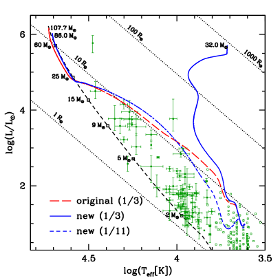
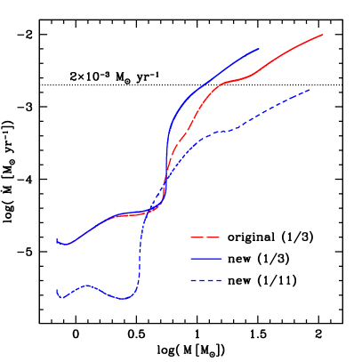
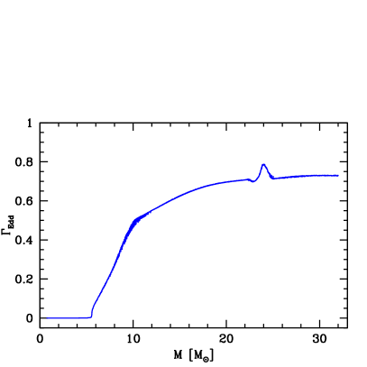
As in the case with a constant accretion rate (Sect. 3), both models remain essentially identical in the low-mass range, while the star is fully convective. But again, when the star enters the intermediate-mass range, becomes radiative, and starts its swelling, the two models diverge; the new model has a higher radius and luminosity than the original model (Fig. 7). However, in this case, the dependence of the accretion rate on the stellar luminosity produces a positive feedback: the rapid increase in luminosity in the new model leads to a rapid increase in its accretion rate (see Fig. 8). In this model, the accretion rate reaches $10^{-3}\,M_{\odot}\rm\,yr^{-1}$ already in the intermediate-mass range (at $M=7.3\,M_{\odot}$), while in the original model it is reached only in the high-mass range (at $M=10.6\,M_{\odot}$). As a consequence, the swelling is enhanced in the new model compared to the original one, leading to radii as high as $100\,R_{\odot}$ (Fig. 7) at a mass of $10.2\,M_{\odot}$. At such a mass, which corresponds roughly to the beginning of the high-mass range, the swelling slows down, but before the star can contract again, the positive feedback between the stellar luminosity and the accretion rate leads to the critical value of Hosokawa (Fig. 8, at a mass of $11.5\,M_{\odot}$). At this point, the stellar luminosity exceeds 50% of the Eddington luminosity (Fig. 9), and the second swelling occurs (see Sect. 1 or Hosokawa & Omukai 2009; Hosokawa et al. 2010 for more details). As we can see in Fig. 7, during this second swelling, the star goes back to the red until it reaches the boundary of the forbidden region of Hayashi, as in the case of a red giant. Then, as the swelling goes on, the star moves upwards on the HR diagram, along a vertical line, similar to the red giant branch (i.e. it moves up the Hayashi line). We stopped the computation when the stellar mass was $32\,M_{\odot}$ with a radius approaching $1000\,R_{\odot}$ and a luminosity close to 75% of the Eddington luminosity (Fig. 9). If we stop accretion at this point, the star simply contracts towards the ZAMS in a Kelvin-Helmholtz time ($45\,000\rm\,yr$ for such a mass), as in the canonical scenario of pre-MS at constant mass. It shows that the canonical scenario corresponds to the limit of the accretion scenario for a high accretion rate.

Figure 9: Eddington factor as a function of the stellar mass, for the model “new (1/3)” of Fig. 7, i.e. of the model computed with the accretion rate of Eq. (19) with $f=1/3$ using the new version of the code (Sect. 2), starting from the initial model given by Eq. (20).

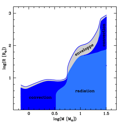
The internal structure of this model is shown in Fig. 10. Until the end of the first swelling, the internal structure is similar to the cases of constant accretion rates described in Sect. 3. But when the second swelling occurs, the convective envelope comes back, as in the case of a red giant or in the initial model of a $\sim 30\,M_{\odot}$ star in the canonical scenario.

Figure 10: Evolution of the radius (upper blue curve) and the internal structure of the model “new (1/3)” of Fig. 7, i.e. of the model computed with the accretion rate of Eq. (19) with $f=1/3$ using the new version of the code (Sect. 2), starting from the initial model given by Eq. (20). The dark blue areas are convective zones, the light blue areas are radiative regions, and the grey area is the envelope (see footnote 4).

The new birthline computed with $f=1/3$, if representative of the birthline for the majority of stars, would predict a much more extended distribution than the one observed for the pre-MS stars. In the next section we discuss a birthline obtained with a lower value of $f$, which produces an upper envelope more compatible with the observations.

4.3 Model with $f=1/11$

We computed a third birthline with the new version of the code, the same initial model, and the Churchwell-Henning accretion rate, but with a value of $f=1/11$ (i.e. $(1-f)/f=10$). The evolutionary track of this birthline is shown in Fig. 7 (blue dashed line), and the corresponding accretion history is in Fig. 8.

As we can see, thanks to the low value of $f$, the accretion rate of this new birthline is lower than in the other two cases by nearly one order of magnitude. This new birthline diverges rapidly from the other two already in the low-mass range, but when the star enters the intermediate-mass range, the swelling brings the new birthline back to the original one (see Fig. 7). Then, the two birthlines remain close to each other until the end of the computation at masses above $85\,M_{\odot}$. In particular, with this new birthline, we can also reach such high masses still close to the ZAMS.

4.4 Discussion

As we can see by looking at the two new birthlines in Sects. 4.2 and 4.3 (blue tracks in Fig. 7), if we want to reproduce the original birthline, which is in agreement with the observations in the whole stellar-mass range, it is necessary to consider a value of $f$ that decreases with the stellar mass. With the original value of $f=1/3$, we still obtain a satisfactory result in the low-mass range, but in the intermediate- and high-mass range, such a high value of $f$ leads to luminosities that are too high compared to those of Herbig Ae/Be stars. If such an accretion history was realistic, we would expect to observe massive pre-MS stars contracting towards the ZAMS at such high luminosities, which is not the case. Inversely, if we consider the value $f=1/11$, in the low-mass range we obtain an accretion rate that is much lower than the typical rate of $10^{-5}\,M_{\odot}\rm\,yr^{-1}$ expected for such masses (e.g. Stahler et al. 1980a, b). With this accretion rate, we obtain luminosities that are too low compared to the observed T Tauri stars, as can be seen in Fig. 7. But in the intermediate- and high-mass range, this new value of $f$ leads to a birthline that is in good agreement with the observations, fitting the upper envelope of Herbig Ae/Be stars and allowing us to produce stars of masses above $80\,M_{\odot}$ still close to the ZAMS. Interestingly, this value is also in good agreement with the observational estimations of Churchwell (1999) for B-type stars, which corresponds to the intermediate-mass range. As a consequence, our results suggest that the efficiency of accretion from a disc decreases with the stellar mass: the higher the stellar mass, the larger the fraction of the material coming from the disc that is rejected through the bipolar outflows.

The assumption of a unique accretion history is certainly an approximation, and we expect the real accretion histories of stars to depend on the final mass they are destined to reach. In this sense, each of our birthlines has to be seen as an upper envelope of the evolutionary tracks of each individual accreting star, corresponding to the main accretion phase (Maeder 2009). Even in this case, however, the value of $f$ during the main accretion phase has to be lower for stars of intermediate- and high-mass than for low-mass stars in order to reproduce the upper envelope of observed pre-MS stars.

We note that when we compute the accretion rate from the luminosity with Eq. (19), we do not include the accretion luminosity $L_{\rm accr}$. This additional contribution would increase the accretion rate, leading to a higher birthline on the HR diagram. In order to keep the birthline in agreement with the observations, we would need to reduce the value of $f$. Thus the value $f=1/11$ has to be seen as an upper limit for the intermediate- and high-mass range. Moreover, $L_{\rm accr}$ represents a larger fraction of the total luminosity $L_{\rm tot}=L+L_{\rm accr}$ in the low-mass range than in the intermediate- and high-mass ranges. In the low-mass range, $L_{\rm accr}\simeq 90\%L_{\rm tot}$ typically, while in the intermediate- and high-mass ranges $L_{\rm accr}\lesssim 50\%L_{\rm tot}$. As a consequence, taking into account the accretion luminosity would reduce the decrease of $f$ as a function of $M$.

Another issue is the dependence of these results on the initial model. In Sect. 3.2 we showed that for a constant accretion rate of $10^{-3}\,M_{\odot}\rm\,yr^{-1}$ the choice of the initial model has a critical impact on the evolution. However, in the case of the Churchwell-Henning accretion law for $f=1/11$, the accretion rate remains much lower than $10^{-3}\,M_{\odot}\rm\,yr^{-1}$ during the whole pre-MS phase (Fig. 8), and it turns out that the shape of this birthline is nearly unchanged when we use the initial model RC of Sect. 3.2 instead of the initial model given by Eq. (20). In other words, the choice of the initial model has no significant influence on the results of the present section.

4.5 Main sequence evolution and isochrones

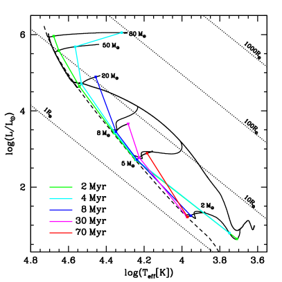
Usually, MS models are computed starting from the ZAMS with initial conditions obtained from canonical pre-MS at constant mass. However, Bernasconi & Maeder (1996) obtained in their models that the internal structure of a MS star is not the same in the accretion scenario as in the canonical scenario. They found that for a given mass and central mass fraction of hydrogen, a MS star formed by accretion has a smaller convective core than a MS star coming from a canonical pre-MS, leading thus to a shorter MS lifetime. In order to see how the pre-MS scenario described in the previous sections modifies the structure and the evolution of MS stars compared to canonical MS models, we computed contractions at constant masses from the birthline described in Sect. 4.3 (Churchwell-Henning accretion rate with $f=1/11$), and the subsequent MS evolution. We obtain that the internal structure on the ZAMS and the evolution on the MS are identical to those of canonical MS stars. The HR tracks of the contractions for $M=2$, 5, 8, 20, 50, and $80\,M_{\odot}$ and the subsequent MS tracks are shown in Fig. 11. We also added several isochrones of 2, 4, 8, 30, and 70 Myr. A more complete grid with isochrones will be available in a forthcoming paper.

Figure 11: HR tracks of the birthline “new(1/11)” (Sect. 4.3), and the subsequent contractions and MS tracks for $M=2$, 5, 8, 20, 50, and $80\,M_{\odot}$ (solid black lines). Several isochrones are indicated with coloured solid lines. The iso-radius of 1, 10, 100, and $1000\,R_{\odot}$ are indicated with black dotted lines and the ZAMS of Ekström et al. (2012) is shown with a black dashed line.

5 Conclusions and perspectives

We showed that the previous versions of the code contained an inconsistency that lead to an artificial loss of entropy in the case of an accreting star dominated by the radiative transport. As a result of this artificial loss of entropy, we underestimated the magnitude of the swelling that occurs when an intermediate-mass star accretes at a high rate ($\sim 10^{-3}\,M_{\odot}\rm\,yr^{-1}$). With the new version of the code, we obtain results that are in good agreement with those of other authors, provided that we compare models with the same physical conditions. In this context, we showed that the existence of a significant swelling that brings the star back towards the red part of the HR diagram, as described by other authors, depends critically on the initial conditions.

We looked at the effects of these improvements on the accretion history given by the Churchwell-Henning relation and considered various values of $f$, the fraction of the material coming from the disc which is effectively accreted by the star. Using the original value of $f=1/3$, we found that the first swelling of the star leads to a radius of $100\,R_{\odot}$; before the star can contract again, a second swelling occurs, which leads the star to the red part of the HR diagram until the boundary of the forbidden region of Hayashi with radii near $1000\,R_{\odot}$ and a new convective envelope. We showed that instead, with a fraction $f=1/11$, the birthline remains close to the original birthline of Behrend & Maeder (2001) in the intermediate- and high-mass range. This new value of $f$ is in good agreement with the estimations of Churchwell (1999) and provides a good fit to the observed upper envelope of pre-MS stars in the HR diagram for luminosities higher than about 2.5. At lower luminosities, a value of $f$ equal to 1/3 gives a better fit. Therefore, in order to reproduce these observations with the new version of the code, we conclude that it is necessary to consider a fraction $f$ that decreases with the stellar mass, which suggests that, when the stellar mass increases, the mass that is accreted represents a still smaller fraction of the mass that is in the outflows.

In the next paper in this series we will add the effects of rotation. Since pre-MS models simultaneously including the effects of accretion and rotation and computed with the original version of the code have been published (Haemmerlé et al. 2013), we will describe how the new improvements modify the results in the case of rotation.