Improved grand canonical sampling of vapour-liquid transitions

Abstract

Simulation within the grand canonical ensemble is the method of choice for accurate studies of first order vapour-liquid phase transitions in model fluids. Such simulations typically employ sampling that is biased with respect to the overall number density in order to overcome the free energy barrier associated with mixed phase states. However, at low temperature and for large system size, this approach suffers a drastic slowing down in sampling efficiency. The culprits are geometrically induced transitions (stemming from the periodic boundary conditions) which involve changes in droplet shape from sphere to cylinder and cylinder to slab. Since the overall number density doesn’t discriminate sufficiently between these shapes, it fails as an order parameter for biasing through the transitions. Here we report two approaches to ameliorating these difficulties. The first introduces a droplet shape based order parameter that generates a transition path from vapour to slab states for which spherical and cylindrical droplet are suppressed. The second simply biases with respect to the number density in a tetragonal subvolume of the system. Compared to the standard approach, both methods offer improved sampling, allowing estimates of coexistence parameters and vapor-liquid surface tension for larger system sizes and lower temperatures.

1 Introduction

An order parameter for a discontinuous phase transition is any quantity which distinguishes clearly between the states that coexist on the phase boundary. For magnets this is usually taken to be the magnetisation, while for the vapour-liquid (VL) transition of a single component fluid an appropriate choice is the overall number density $\rho=N/V$. A particularly successful approach for studying VL phase transitions utilizes grand canonical Monte Carlo (GCMC) simulation to study the probability distribution $p(\rho)$ of the fluctuating density [1]. Precisely at coexistence, $p(\rho)$ exhibits a pair of equally weighted peaks which are centred on the densities of the coexisting phases. These peaks are separated by a deep probability valley as is illustrated in Fig. 1 which displays the coexistence form of $\ln p(\rho)$ for the three dimensional (3d) Lennard-Jones (LJ) fluid at a strongly subcritical temperature. For sufficiently large system size and/or sufficiently low temperature, the valley exhibits a flat linear region corresponding to liquid slab configurations in which the liquid spans the periodic boundaries in $d-1$ dimensions and is separated from the vapor by a planar interface in the remaining dimension. Since the free energy is related to the probability distribution by $\beta f(\rho)=-\ln p(\rho)$, the valley flatness reflects the equality of the free energy of the coexisting phases, there being no cost involved in altering the width of the liquid slab.

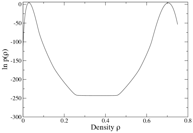
Figure 1: Estimates of the logarithm of the number density distribution $p(\rho)$ for the 3d LJ fluid at $T=0.775T_{c}$. The system volume is $V=(17.5\sigma)^{3}$. Note the equality of the peak weights and the deep probability valley, which is flat in the region for which liquid slab states occur. The distribution was obtained using MUCA biased with respect to the density $\rho$.

Slab configurations differ in free energy from a pure phase vapor (or a liquid) by the free energy cost of inserting a pair of vapor-liquid interfaces. Accordingly, the probability ratio of pure phase and slab states provides an accurate means of measuring the vapor-liquid surface tension [2, 3]. Specifically one finds for a 3d system of volume $V=L^{3}$,

$$\gamma_{vl}=(2\beta L^{2})^{-1}\ln(p_{\rm max}/p_{\rm min})\>,$$ (1)

where $\beta=(k_{B}T)^{-1}$ and $p_{max}\equiv p_{\rm vap}=p_{\rm liq}$ is the height of the peaks of $p(\rho)$.

Thus, in principle at least, GCMC estimates of $p(\rho)$ provide a route to determining both coexistence parameters (via the equality of peak weights or the flatness of the valley bottom) and vapor-liquid surface tension (via the peak to valley height). However the probability valley separating the two pure phases represents a serious obstacle to efficient MC sampling of the distribution. For modest system sizes this can be overcome using Multicanonical sampling (MUCA). MUCA is a biasing scheme for first order phase transitions which was first introduced in the context of lattice based spin models [4]. It was subsequently generalized to GCMC studies of fluid phase transitions [1] and used to study a wide variety of fluid models including some originally introduced by George Stell [5, 6, 7].

To recall how MUCA works with GCMC, consider a fluid system specified by a set of $N$ particles and their coordinates ${\bf r}^{N}$. MUCA samples not from the true Hamiltonian ${\cal H}({\bf r}^{N})$ but from a modified one

$${\cal H}^{\prime}({\bf r}^{N})={\cal H}({\bf r}^{N})+\eta({\bf r}^{N})\>,$$ (2)

where $\eta({\bf r}^{N})$ is a user defined weight function. In the original GCMC formulation [1], the weights $\eta({\bf r}^{N})$ were simply defined with respect to the overall density ie. $\eta({\bf r}^{N})=\eta(\rho)$. It is straightforward to show [8] that the choice $\eta(\rho)=-f(\rho)$ leads to uniform sampling of the density range. Of course, generally one doesn’t know the form of $f(\rho)$ a-priori. Nevertheless iterative [9, 10] or transition matrix methods [11] allow the determination of a good approximate form which should result in near-uniform sampling. Once such a preweighted simulation has been performed, it is a simple matter to unfold the bias [4, 8] to determine the requisite form of $p(\rho)$. GCMC in conjunction with density-weighted MUCA has been successful in yielding the form of $p(\rho)$ at VL phase transitions for moderate system sizes [1, 3]. However, for large system sizes and particularly at low temperatures, further sampling difficulties arise due to so-called droplet transitions for which $\rho$ does not provide a good order parameter for biasing purposes, as we now describe.

2 Droplet transitions and sampling issues

Droplet transitions are geometrically induced first order phase transitions which occur in systems that have periodic boundary conditions. They were first recorded in the context of the 2D Ising model [12]. For 3d fluids and for sufficiently system volumes, three droplet states are observed. As the density is raised above that of a homogeneous vapour, a state with a spherical droplet occurs. Further increasing the density results in a cylindrical droplet whose ends are connected via the periodic boundary conditions of the simulation box. Finally, at larger densities a tetragonal slab configuration is formed. At even higher densities than those at which slabs occur, a set of analogous ‘bubble’ transitions occur involving spherical and cylindrical bubbles [13, 14].

Droplet transitions in fluids are of interest in their own right both for the information they provide concerning curvature corrections to the surface tension and for their finite-size scaling properties [15, 13, 16, 17]. Signatures of the droplet transitions are visible in $p(\rho)$ which exhibits kinks and rounded discontinuities at the densities for which the transitions occur [13, 16]. The kink at the cylinder-slab transition is particularly pronounced (cf. fig. 1 for $\rho\approx 0.26$). Unfortunately, for large systems sizes and low temperatures, droplet transitions cause serious sampling difficulties. These were first studied in the context of MUCA simulations of the 2d Ising model where a finite-size scaling analysis [18] found that they lead to slowing down which is exponential in $\beta L^{d-1}$. Similar problems arise in fluids [19] and are manifest in the fact that even if one finds a weight function $\eta(\rho)$ that leads to uniform sampling of the density domain, the sampling becomes ‘stuck’ in regions of density associated with one type of droplet. Fig. 2 illustrates this problem for the LJ fluid. The root cause is that the density $\rho$ does not discriminate sufficiently between the various droplet states, so biasing with a weight function $\eta(\rho)$ fails as a means for traversing the transitions.

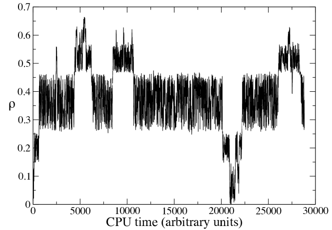
Figure 2: A trajectory of a MUCA simulation of the LJ fluid at $T=0.775T_{c}$ biased with respect to $\rho$. The volume is $V=(20\sigma)^{3}$. Spheres occur in the density range $\rho\approx 0.07-0.15$; cylinders for $\rho\approx 0.15-0.26$, and slabs for $\rho\approx 0.26-0.46$. At still higher densities cylindrical and spherical bubble states occur.

A number of ways of tackling this problem have been considered previously. One is to augment the sampling with transitions to higher temperatures where the barriers between transitions are smaller, which can be achieved using expanded ensembles or parallel tempering [20, 21]. Although this is reported to help, it seems rather cumbersome and laborious, particularly for very low temperatures. Another approach is to modify the system geometry in order to remove the periodic boundaries that cause droplet transitions. This has been tried in the case of a 2D fluid by simulating it on the surface of a sphere [19]. Doing so appears to eliminate sampling barriers, but the use of curved non-Euclidean space leads to non-trivial finite-size effects which seem to affect calculations of surface tension in particular. Moreover the extension to three dimensional systems seems complicated because it involves simulating the system on the surface of a hypersphere.

A different way to try to tackle the sampling issues associated with droplet transitions is to recognize that MUCA is not restricted to weight functions that are defined solely with respect to simple macrovariables such as the density or energy; any function of the configurational coordinates can be used. Thus, for instance, work has been done to try to find a smooth path between liquid and solid phases by biasing with respect to an order parameter which is related to the degree of local crystalline order in the system [22]. In the present contribution we look at two approaches based on non-standard order parameters and apply them to the VL transition of a LJ fluid. Our first order parameter comprises a linear combination of moments of the configuration shape and is designed to create a sampling path between vapour and slab states that suppresses spherical and cylindrical droplets. Our second method is inspired by the insights gained from the first and simply uses the density in a tetragonal subvolume of the system as the order parameter. Both methods improve the sampling, though the second is considerably faster and easier to implement. In the following we describe the methods in turn and test their efficacy.

3 Linear combination of moments

We consider a GCMC simulation of an orthorhombic simulation cell of dimensions $L_{x},L_{y},L_{z}$ with periodic boundary conditions. For any configuration ${\bf r}^{N}$ one may calculate three geometrical second moments with respect to the orthogonal box axes

$$m_{x} = \sum_{i}^{N}(x_{i}-\bar{x})^{2}$$ (3a)

$$m_{y} = \sum_{i}^{N}(y_{i}-\bar{y})^{2}$$ (3b)

$$m_{z} = \sum_{i}^{N}(z_{i}-\bar{z})^{2}$$ (3c)

where ${\bf r_{i}}=(x_{i},y_{i},z_{i})$ is the position vector of particle $i$ and $\bar{x},{\bar{y}},{\bar{z}}$ are the components of the centre of mass (COM). Our first order parameter is based on these moments. To calculate them we need to determine the COM. However, this is not trivial to calculate for a periodic system. The definition appropriate to infinite space ($\bar{x}=N^{-1}\sum_{i}^{N}x_{i}$, etc.) clearly fails for a periodic system as is readily appreciated by considering the case of a single cluster which is split across the periodic boundary. To circumvent this problem, Bai and Breen [23] have introduced an efficient scheme which averages the coordinates in a higher dimensional space. The method works by mapping each dimension of the simulation box onto a unit circle in the two-dimensional (2D) plane and performing averages in this plane. Specifically, for the determination of ${\bar{x}}$ one calculates, for each particle $i$, an angle in the interval $(0,2\pi)$:

$$\theta_{i}=2\pi(x_{i}/L_{x})\>.$$ (3d)

The corresponding point on a unit circle has 2D coordinates

$$\chi_{i} = \cos(\theta_{i}),$$ (3ea)

$$\psi_{i} = \sin(\theta_{i})\>.$$ (3eb)

One calculates the average of these coordinates for the full set of $\{\theta_{i}\}$

$$\bar{\chi} = \frac{1}{N}\sum_{i}^{N}\chi_{i},$$ (3efa)

$$\bar{\psi} = \frac{1}{N}\sum_{i}^{N}\psi_{i}\>.$$ (3efb)

Then the average coordinates $\bar{\chi}$ and $\bar{\psi}$ are extended back onto the unit circle to generate a new angle

$$\bar{\theta}=\arctan 2(-\bar{\psi},-\bar{\chi})+\pi\>.$$ (3efg)

Finally, mapping this angle back on to the $x$-axis of the simulation box yields the $x$-component of the centre of mass as

$${\bar{x}}=(\bar{\theta}/2\pi)L_{x}\>.$$ (3efh)

Analogous calculations for the $\{y_{i}\}$ and $\{z_{i}\}$ yield the ${\bar{y}}$ and ${\bar{z}}$ components of the COM.

While this calculation of the COM is more complex than the naive one, changes to the COM in the GCE as particles are added or deleted can be calculated very efficiently because one need only keep track of the changes to the sums $\sum_{i}\chi_{i}$ and $\sum_{i}\psi_{i}$ appearing in Eq. 3efb.

Unfortunately matters are not quite so straightforward with regards to calculating the moments themselves. For an infinite system one can expand

$$m_{x}=\sum_{i}^{N}(x_{i}-\bar{x})^{2}=\sum_{i}x_{i}^{2}-2\bar{x}\sum_{i}x_{i}+N\bar{x}^{2}$$ (3efi)

and play a similar trick of calculating changes in the moments due to a shift in the centre of mass by keeping track of changes to the sums when we insert or delete particles. However for a finite periodic system we should apply the minimum image convention to the displacement $x_{i}-\bar{x}$ before we square it and sum. Since the COM $\bar{x}$ wanders during the simulation this requires, in principle, a recalculation of the displacements following each insertion or deletion. This is a potentially expensive calculation, albeit one which is only $O(N)$ in complexity. To reduce the cost we divide our particles into two sets, those that are nearer the COM than some prespecified radius, and those that are outside this radius. For each insertion and deletion we only check particles outside the radius whether the minimum image convention needs to be applied. For those inside the radius we calculate the contribution to the moments immediately by exploiting the expansion Eq. 3efi ie. by keeping track of the partial sums and the COM.

Having calculated the moments $m_{x},m_{y},m_{z}$ for a given configuration, we order them according to magnitude from the smallest to the largest and relabel them $a$, $b$ and $c$ respectively. Clearly for a configuration which is in a spherical droplet state one has on symmetry grounds that $a\approx b\approx c$; for a cylinder one has $a<b\approx c$, while for a slab $a\approx b<c$. We now define the order parameter for our system as a linear combination of $a$,$b$ and $c$. Specifically we write

$${\cal M}\equiv c-\beta b-\alpha a\>,$$ (3efj)

where $\alpha>0,\beta>0$ and $\alpha+\beta<1$. We refer to ${\cal M}$ as the linear combination of moments (LCM) order parameter. It gives rise to a one-dimensional weight function $\eta({\cal M})$. The rationale for the definition of this order parameter is to alter the reaction coordinate in order to bypass the formation of spheres and cylinders, but not slabs. To appreciate how this can work, consider the case $\alpha=0,\beta=1$. For this choice spheres and cylinders occur for ${\cal M}\approx 0$, but since the vapor state also has ${\cal M}\approx 0$ and has a lower free energy than spheres and cylinders, these droplet states will be suppressed.

Clearly the LCM order parameter requires a greater computational effort to calculate than a simple macrovariable such as the density or energy. Nevertheless, we find that this additional cost is more than offset by improved sampling efficiency at vapour-liquid transitions. In fig. 3 we compare the sampling efficiency of MUCA simulations using the density order parameter and the LCM order parameter for a system of size $L=20\sigma$, which is the largest for which one can observe droplet state transitions on a reasonable time scale. The figure shows the evolution of the density as a function of CPU time in arbitrary units. For the LCM order parameter many more round trips of the density range occur per unit time than for the density order parameter. It is therefore more efficient at finding the relative weight of vapor and slab states which is necessary for accurate estimates of the surface tension.

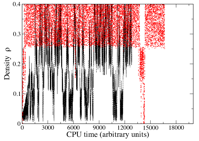
Figure 3: Comparison of typical trajectories of the overall density $\rho$ as a function of CPU time (in arbitrary units) for the density order parameter (points) and the LCM order parameter (lines). The LCM parameters (cf. Eq. 3efj) are $\beta=0.9,\alpha=0.1$. Clearly the barriers to sampling are much reduced for the LCM method. The system volume is $V=(20\sigma)^{3}$ and the temperature is $T=0.775T_{c}$.

The LCM order parameter and the density order parameter guide the system along different configuration space paths. This becomes apparent when one unfolds the weights from simulations performed using the respective order parameters to obtain the forms of $p(\rho)$. These are compared in Fig. 4 for a system of volume $V=(17.5\sigma)^{3}$ (which is the largest for which $p(\rho)$ can reliable be determined using the density order parameter). The two distributions coincide in the region of the vapor peak and in the (flat) region where slabs occur. However they differ at intermediate densities because in the LCM case spheres and cylinders are suppressed. Examination of configuration snapshots reveals that for the LCM order parameter, the transition path favours configurations which have slab-like moments from the outset. At small $\rho$, however, there are too few particles to form a true slab and instead the system adopts a rather complex arrangement in which two or more spherical droplets are arranged across the diagonal of a notional slab. In view of this it seem that the LCM method does not eliminate droplet transitions altogether, although it does appear to provide a significantly smoother sampling path from vapor to slab than the traditional density order parameter.

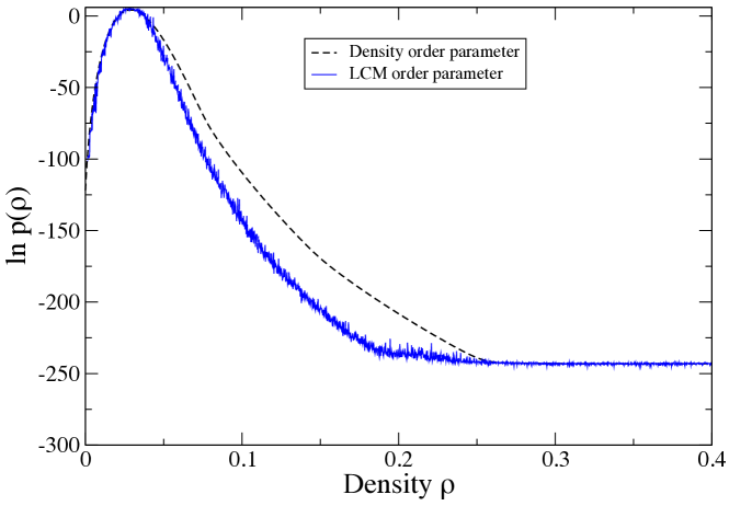
Figure 4: Comparison of the logarithm of $p(\rho)$ determined from MUCA simulations biased with respect to the density order parameter and the LCM order parameter, as discussed in the text. The system volume is $V=(17.5\sigma)^{3}$ and the temperature is $T=0.775T_{c}$.

4 Biasing on a subvolume density

We have seen that the LCM parameter engineers a smoother path between vapor and liquid slab configurations by promoting configurations which (at least in the sense of the relative magnitudes of the moments describing their shape) are slab-like at all densities. This suggest a simpler approach in which one increases the density from vapor-like values by directly creating slab-like configurations. To this end we implement MUCA with a bias defined on the number density $\rho_{s}=N_{s}/V_{s}$ of particles in a tetragonal subvolume of dimensions $V_{s}=L_{x}\times L_{y}\times d_{z}.$. Here the subvolume width $d_{z}$ is a parameter which we set to lie in the range $5\sigma-7.5\sigma$. This value is chosen to yield a slab that is sufficiently thick that it is stable against capillary wave fluctuations of the VL interface, but sufficiently narrow that spheres and cylinders cannot be comfortably accommodated within the subvolume.

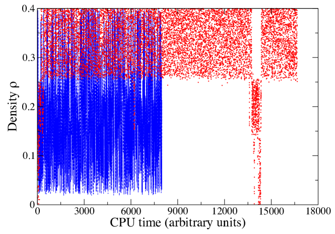
Figure 5: Comparison of typical trajectories of the overall density as a function of time for MUCA simulations biased with respect to the overall density (points) and the subvolume density (lines). Clearly the sampling efficiency is greatly increased in the latter case. The system volume is $V=(20\sigma)^{3}$ and the temperature is $T=0.775T_{c}$.

By avoiding the costly moment calculation, simulations using the subvolume density order parameter run about an order of magnitude faster than the LCM approach. A comparison of sampling efficiency presented in Fig. 5 shows that the subvolume approach reproduces the smoother sampling path between vapor and liquid-slab densities seen in the LCM case, but the CPU time taken to traverse this density range is only about $1\%$ of that required when using the overall density order parameter. Use of the subvolume approach therefore results in sampling which is about two orders of magnitude faster than the standard density order parameter approach for the system size studied. Like the LCM method, the subvolume density order parameter method yields the same values of $p_{max}$ and $p_{min}$ as does the overall density order parameter and can therefore be used to calculate surface tension.

The LCM method is based on geometrical moments of droplet configurations which occur for densities between those of the pure vapor and liquid slab configurations. At higher densities bubble states appear which cannot be usefully characterised via the LCM order parameter. By contrast the subvoume method can be used to traverse the density range from vapor to slab and (separately) the density range from slabs to pure liquid for which bubble transitions occur. To do so one needs to calculate a separate MUCA weight function depending on whether one is aiming to form a liquid slab within the vapor phase or a vapor-like slab within the liquid phase. This ability to cover the whole density range between vapor and liquid (albeit in two stages) is a further reason to prefer the subvolume order parameter over the LCM one.

However, in common with the LCM case, the subvolume density order parameter does not eliminate droplet transitions. This can be seen by considering an even larger system size, $V=(25\sigma)^{3}$. Examination of a typical trajectory (Fig. 6) reveals the emergence of sampling barriers, the scale of which we expect to grow strongly with increasing system size.

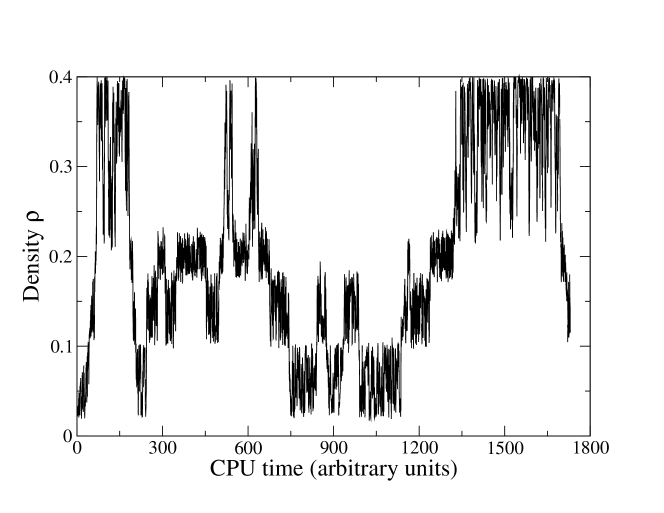
Figure 6: A typical trajectory for the subvolume density method for $V=(25\sigma)^{3}$. Barriers to smooth sampling are clearly visible at this system size indicating the presence of droplet transitions.

5 Conclusions

In summary we have considered strategies for improving the efficiency of multicanonical simulations of liquid vapor transitions at low temperatures and large system sizes. Standard simulations based on biasing with respect to the overall density suffer sampling difficulties due to droplet transitions. We have considered two alternative one-dimensional order parameters which ameliorate these problems. One is based on a linear combination of the second moments of the configuration geometry, the other is based on a subvolume density. While both order parameters seem to reduce the height of sampling barriers to a similar degree, the subvolume density method is preferable because it is easier to implement, more versatile, and entails little or no computational overhead compared to biasing on the total density. We expect that both order parameters will be applicable to lattice based spin systems where droplet transitions also occur.

Although we have shown that alternative order parameters can reduce the free energy barriers that cause slowing down, they clearly do not eliminate them. The sphere-cylinder and cylinder-slab droplet transitions are replaced by other transitions involving more complex droplet geometries. It therefore remains the matter of further work to devise better strategies that completely solve the sampling issues that afflict GCMC at low temperatures and large systems sizes.

References

- [1] Wilding N B 1995 Phys. Rev. E 52 602–611
- [2] Binder K 1982 Phys. Rev. A 25(3) 1699–1709
- [3] Errington J R 2003 Phys. Rev. E 67 012102
- [4] Berg B A and Neuhaus T 1992 Phys. Rev. Lett. 68(1) 9–12
- [5] Pini D, Stell G and Wilding N B 2001 J. Chem. Phys. 115(6) 2702–2708
- [6] Magee J E and Wilding N B 2002 Molecular Physics 100(10) 1641–1644
- [7] Gibson H M and Wilding N B 2006 Phys. Rev. E. 73 061507
- [8] Bruce A D and Wilding N B 2003 Adv. Chem. Phys 127 1
- [9] Berg B 1996 J. Stat. Phys. 82 323
- [10] Virnau P and Müller 2004 J. Chem. Phys. 120 10925–10930
- [11] Smith G R and Bruce A D 1995 J. Phys. A 28(23) 6623–6643
- [12] Leung K and Zia R K P 1990 J. Phys. A 23 4593
- [13] MacDowell L G, Shen V K and Errington J R 2006 J Chem Phys 125 34705
- [14] Archer A and Wilding N 2007 Phys. Rev. E 76 031501
- [15] MacDowell L G, Virnau P, Müller M and Binder K 2004 J. Chem. Phys. 120 5293–5308
- [16] Binder K, Block B J, Virnau P and Tröster A 2012 Am. J. Phys. 80 1099–1109
- [17] Zierenberg J and Janke W 2015 Phys. Rev. E 92(1) 012134
- [18] Neuhaus T and Hager J 2003 J. Stat. Phys. 113 47–83
- [19] Fischer T and Vink R L C 2010 J. Phys.: Condens. Matter 22 104123
- [20] Grzelak E M and Errington J R 2010 Langmuir 26 13297–13304
- [21] Neuhaus T, Magiera M P and Hansmann U H E 2007 Phys. Rev. E 76(4) 045701
- [22] Chopra M, Müller M and de Pablo J J 2006 J. Chem. Phys. 124 134102
- [23] Bai L and Breen D 2008 Journal of Graphics, GPU, and Game Tools 13 53–60