Predicting Coronal Mass Ejections transit times to Earth with neural network

Abstract

Predicting transit times of Coronal Mass Ejections (CMEs) from their initial parameters is a very important subject, not only from the scientific perspective, but also because CMEs represent a hazard for human technology. We used a neural network to analyse transit times for 153 events with only two input parameters: initial velocity of the CME, $v$, and Central Meridian Distance, CMD, of its associated flare. We found that transit time dependence on $v$ is showing a typical drag-like pattern in the solar wind. The results show that the speed at which acceleration by drag changes to deceleration is $v\approx$500 km s^-1. Transit times are also found to be shorter for CMEs associated with flares on the western hemisphere than those originating on the eastern side of the Sun. We attribute this difference to the eastward deflection of CMEs on their path to 1 AU. The average error of the NN prediction in comparison to observations is $\approx$12 hours which is comparable to other studies on the same subject.

1 Introduction

Coronal mass ejections (CMEs) are important drivers of space weather. They can cause strong geomagnetic storms (Gosling et al., 1990, 1991; Zhang et al., 2003; Echer et al., 2008; Richardson & Cane, 2012; Cid et al., 2014). Zhang et al. (2007) concluded that 87% of strong geomagnetic storms were caused by either a single CME or multiple interacting CMEs, while Richardson, Cliver & Cane (2001) attribute 97% of the most intense storms to transient structures associated with CMEs. Another significant cause of geomagnetic storms are corotating interactive regions (CIRs) (see Alves, Echer & Gonzalez 2006 and references therein). CME-associated events can cause serious damage to communication and navigation satellites, threaten the safety of astronauts, and in most extreme cases can disrupt electric power supply on the ground (Boteler, Pirjola & Nevanlinna, 1998; Schrijver & Mitchell, 2013). Solar energetic particle (SEP) events accelerated by CME-driven shocks also present a risk to equipment and humans in space (see Dierckxsens et al. 2015 and references therein). A more detailed summary of space weather hazards is given in Feynman & Gabriel (2000).

Predicting when CMEs will reach the Earth is thus very important. Typical transit times ($TT$) for CMEs to reach the Earth are between 1 and 5 days (Richardson & Cane, 2010). In this paper, we use CME to refer to CMEs both near the Sun and interplanetary space (often called interplanetary coronal mass ejections (ICMEs) in other studies). Furthermore, observed transit times are based on the arrival of the leading edge of the CME/ICME. Understanding how the $TT$ depends on initial properties of the CME and the associated phenomena is the most promising way of getting an early warning for a possible geomagnetic storm. Unsurprisingly, velocity of the CME in the LASCO field of view was found to be one of the most significant parameters. Schwenn et al. (2005) derived an empirical logarithmic expression for $TT$ as a function of the expansion velocity of CME for 75 events. The standard deviation of the fit was about 14 hours. Gopalswamy et al. (2001) derived a semi-empirical model of $TT$s based on an effective interplanetary acceleration and CME initial speed. Fry et al. (2003) compared the $TT$ predicted by three different theoretical models and found that the average error of all models is between 11 and 12 hours.

Vršnak et al. (2004) have studied the kinematics of more than 5000 CMEs between 2 and 30 solar radii. They have shown that even close to the Sun the motion of CMEs is affected by aerodynamic drag through the interaction with the ambient plasma. Drag based model (Vršnak & Žic, 2007; Vršnak et al., 2013) was a logical extension of this idea into interplanetary space where the drag force is even more dominant as gravity and Lorentz force weaken further away from the Sun. Recently, Vršnak et al. (2014) compared $TT$ predictions from the Drag Based Model (DBM) and WSA-ENLIL+Cone Model (Odstrcil, Riley & Zhao, 2004; Taktakishvili et al., 2009). The mean value of the difference between calculated $TT$s for the two models was $\overline{\Delta}=0.09\pm 9$ hours, while the average absolute difference from actual observations was $\approx$14 hours for both models. Mays et al. (2015) used ensemble modelling to predict arrival time of CMEs. For the 17 events which did reach the Earth, they found the average absolute error to be $\approx$ 12.3 hours. For a more detailed review of CME $TT$ predictions see Zhao & Dryer (2014).

Another important effect of the ICME propagation through the heliosphere is a deflection from the radial trajectory. Gosling et al. (1987) studied 19 fast CMEs and found a small eastward deflection of about 3°. Wang et al. (2002) found that  60% of geoeffective CMEs occurred on the western solar hemisphere. They attributed this asymmetry to the deflection of CMEs in the interplanetary space. Wang et al. (2004) concluded that CMEs are affected by the Parker’s spiral magnetic field and deflected from the radial trajectory. In their model, fast CMEs are deflected toward east, while slow ones are deflected toward west. By studying latitudinal deflection (North-South direction) of CMEs, Shen et al. (2011) and Gui et al. (2011) developed the magnetic energy density gradient (MEDG) model. In their model, CMEs are deflected to the regions with lower magnetic energy density. Analysing driverless shocks, Gopalswamy et al. (2009) suggested that CMEs are deflected from their radial trajectory by coronal holes (CH). Based on the numerical analysis of the 2005 August 22 event, Lugaz et al. (2011) concluded that the CME was deflected by the CH.

In this work we will use a neural network (NN) to analyse CME $TT$s as a function of CME initial speed and central meridian distance (CMD). Neural networks have many applications and have been successfully used in the analyses of astrophysical problems. For example, Prša et al. (2008) used NN to determine physical properties of eclipsing binaries, Li & Zhu (2013) used it for solar flare forecasting, Valach et al. (2009) for quantifying the geomagnetic response to particular solar events while Uwamahoro, McKinnell & Habarulema (2012) used NN to estimate the geoeffectiveness of halo CMEs. The most advantageous aspect of using NNs for fitting observed data is that it is not necessary to specify any functional form of the empirical curve.

2 Data

We compiled a list of 153 CMEs for which their ICME counterparts were detected and their $TT$ to Earth was measured. We used only the events for which the CME source position could be determined. All CME-ICME pairings were taken from the catalogue provided by Richardson & Cane (2010). For the arrival time of the ICME we used times based on observations of plasma and field. To determine the source position of the CME we consulted a number of papers (Gopalswamy et al., 2001; Zhang et al., 2003; Manoharan, 2006; Zhang et al., 2007; Marubashi et al., 2015) and we also used the automatic method described in Vršnak, Sudar & Ruždjak (2005).

Table 1: Full list of events used in this paper is given as online material.

Start time	Arrival Time	$TT$ [h]	$v$ [km s-1]	Source position
1996 Dec 19 1515	1996 Dec 23 1700	97.74	469	S14W09
1997 Jan 6 1246	1997 Jan 10 0400	87.23	136	S18E06
1997 Feb 7 0017	1997 Feb 10 0200	73.71	490	S20W04
1997 Apr 7 1400	1997 Apr 11 0600	87.98	878	S30E19
1997 May 12 0405	1997 May 15 0900	76.91	464	N21W08
…

As one model parameter we used the CME plane of the sky speed, $v$, which was taken from LASCO coronograph observations for each event. For the positional information about the onset of the CME we used only CMD from the associated flare data in order to investigate if there is an average effect of CMD on $TT$. We assigned negative value of CMD to flares on the eastern hemisphere and positive CMD to those appearing on the western hemisphere of the Sun. For the onset time of the CME we used the linear extrapolation with previously determined speed back to the position of the associated flare. $TT$ is then given by the difference between the arrival time determined by Richardson & Cane (2010) and this onset time. The full event list is included in the supplementary on-line materials; the first few entries are shown in Table 1.

Figure 1: Distribution of velocities and CMDs in parameter space is shown with open circles, while the dotted line marks the smallest convex shape that bounds all the events.

In Fig. 1 we show the distribution of CMEs in our sample in the parameter space spanned by values of their initial velocity, $v$, and CMD. The dotted line in the graph marks the smallest convex shape which includes all the events we used in this work.

3 Neural network method

In this section we give a short overview of NNs and its application to our problem. For a more thorough discussion about NN refer to Gurney (1997) and references therein.

We used a multilayer NN with feed-forward algorithm to transform input to output parameters. Schematic diagram of such a network is shown in Fig. 2. NN takes $k$ input values, $x_{i}$, and through a series of connections transforms the input into one or more output values, $y_{i}$. Between input and output layer there can be one or more hidden layers, although more than two are almost never needed. In Fig. 2 we show the weights as arrows connecting cells (denoted as circles) between different layers.

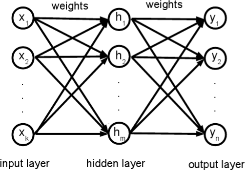
Figure 2: Schematic diagram of a typical feed forward neural network.

To calculate the value in $j$th hidden cell, $h_{j}$, from given input values $x_{i}$ we used the following relation:

$$h_{j}=f\left(\sum\limits_{i=1}^{k}w_{ij}x_{i}\right),$$ (1)

where $w_{ij}$ are weights connecting cells between different layers and $f$ is one of the sigmoid functions (discussed below). Values in the cells of the output layer are calculated in the similar fashion using values in the cells of the hidden layer:

$$y_{j}=f\left(\sum\limits_{i=1}^{m}w_{ij}h_{i}\right).$$ (2)

For the sigmoid function, we have chosen the logistic function:

$$f(x)=\frac{1}{1+e^{-x}}.$$ (3)

Sigmoid function has an ’S’ shape with values bound by asymptotes at $y=0$ and $y=1$ for $x$ between -$\infty$ and $\infty$, respectively. Without the non-linear sigmoid function, the result of the NN would just be an elaborate linear combination of input parameters. Apart from introducing nonlinearity into the method, it also bounds the output from all cells, so in practice input and output parameters are scaled by simple transformations to cover the range of the sigmoid function used. NN performance is not noticeably affected by the choice of the sigmoid function.

As we can see, weights, $w_{ij}$, are previously unknown and represent free parameters of the NN model. If we use past events, known as samples in NN terminology, with measured input and output values we can use backpropagation to optimise the weights. Backpropagation is a form of steepest descent method which slowly optimises weights starting from random values.

Number of weights quickly grows with the number of cells used. By choosing a very large number of cells and, consequently weights, it is possible to create a NN which will perfectly fit all the available data. However, this is clearly not a statistically meaningful procedure. Therefore, the data are divided in at least two samples: learning sample and validation sample. Backpropagation is performed only on the learning sample while the error of the validation sample reveals if we have encountered the overfitting problem. Overfitting is caused when NN describes random noise rather than the underlying relationship. This is typically revealed when the error of the validation sample starts to grow with the increasing number of weights. It is also desirable that average errors of the learning and validation samples have similar values.

From our 153 data points we have grouped 130 of them into the learning sample and the rest into the validation sample. We have also used bias cells in the input and hidden layer. Bias cells are special cells which connect only to forward layers and have a value of one. They are useful for shifting the values of the sigmoid function and in general improve the convergence of the fit. The number of weights, $N_{w}$, is given by:

$$N_{w}=(N_{inp}+1)N_{hid}+(N_{hid}+1)N_{out},$$ (4)

where $N_{inp}$, $N_{hid}$ and $N_{out}$ are the number of cells in input, hidden and output layers, respectively. Bias cells are represented by +1 in both brackets.

Statistical rule of the thumb to pick adequate number of weights is to have the ratio between number of data points and number of weights, $N_{ld}/N_{w}\geq 5$ at least. Of course, the higher the ratio, the results would be more statistically reliable. Ratio of $\approx$10 or higher is recommended.

We used $v$ and CMD as input parameters, while the output parameter was $TT$. By choosing two input cells and one output cell we can see that we are very limited in choosing the number of cells in the hidden layer. We decided to use three cells in the hidden layer which gives an acceptable ratio of $N_{ld}/N_{w}=130/13=10$.

4 Results

4.1 Convergence and errors

In the first step NN assigns random values to weights which typically results in very large differences between calculated and observed output values. Then it uses backpropagation on the learning sample to gradually improve the weights. In Fig. 3 we show the average errors of the learning and the validation sample with increasing number of iterations. We can see that the improvement occurs very quickly at the beginning of the iteration process and after that average errors of both samples stabilise.

Figure 3: Improvement of the average error, $\Delta TT$, with each iteration is shown for the learning sample and the validation sample with a solid and dotted line, respectively.

There is no exact rule when to stop the iterations, so we decided to end the process when errors remain fairly constant for large number of iterations.

We ran this procedure ten times for different learning and validation samples, meaning that samples were made randomly from the full sample of 153 events. The average errors of the learning sample was varying between 10.89 and 11.99 hours, while the average error of the validation sample were between 9.75 and 16.28 hours. This means that, no matter which events are in the learning sample and from which initial random weights the NN starts, the end result is always similar and stable. It also means that our choice of the number of hidden cells was statistically sound.

In Fig. 4 we show distribution of absolute difference between calculated and observed transit times, $|TT_{c}-TT_{o}|$, for the learning sample. The bins are 4 hours wide and we can see that most of the events are contained in the first three bins ($\leq$12 hours).

Figure 4: The distribution of absolute difference between calculated and observed transit times, $|TT_{c}-TT_{o}|$, for the whole sample.

From the ten different runs of NN optimisation we picked the one with the lowest error of the whole sample as the best fit.

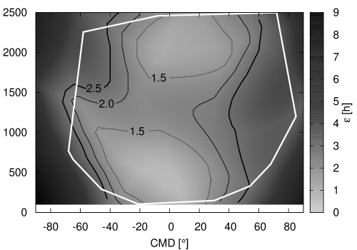
Figure 5: Map plot of error, $\varepsilon(v,CMD)$, based on the best fit NN curve and other nine NN curves (Eq. 5). Thick solid, thin solid and dotted isolines show the contours for $\varepsilon=2.5$ h, $\varepsilon=2.0$ h and $\varepsilon=1.5$ h, respectively. White solid line marks the smallest convex shape bounding all the events.

We can estimate the reliability of the fit by calculating the absolute average differences between best fit values and nine other values found by other NN runs for the full range of input parameters:

$$\varepsilon(v_{m},CMD)=\frac{1}{9}\sum_{i>1}^{10}|TT-TT_{i}|.$$ (5)

In Fig. 5 we show a map plot of $\varepsilon(v_{m},CMD)$ as well as the smallest convex polygon which encloses all the events with the white solid line (see Fig. 1). We can see that errors, $\varepsilon(v,CMD)$, are the smallest within the enclosing polygon. Outside of this polygon errors can become fairly large. This illustrates the problem of extrapolating the results with NN. Extrapolation is almost never recommended with NN and its predictions outside of the input domain are known to be very unreliable.

4.2 Transit times prediction by NN

The most important feature of NNs is the agreement of its calculated values and the actual observations. In Fig. 6 we show calculated and observed $TT$ versus event ID for both the learning and the validation samples.

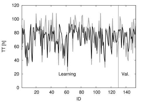
Figure 6: Observed $TT$ (grey line) is shown versus identification number for learning and validation samples. Predicted $TT$ calculated by NN are shown with a black line. Vertical line at 130 delimits the learning from the validation sample.

Observed $TT$ is shown with a thick solid grey line, while $TT$ calculated by NN is shown with a solid black line line. Observed $TT$s as a function of event ID, of course, looks like noise, but we can see that it is closely matched by $TT$s predicted by our NN.

In the ideal case calculated transit times, $TT_{c}$, as a function of the observed transit times, $TT_{o}$, should be a straight line with the functional form $TT_{c}=TT_{0}$.

Figure 7: Calculated, $TT_{c}$, vs observed transit time, $T_{o}$. Function $TT_{c}=TT_{0}$ is shown with the solid line. Filled circles and empty squares are $TT$s from the learning and the validation sample, respectively.

In Fig. 7 we show this relationship. Filled circles and empty squares represent $TT$ values from the learning and the validation samples, respectively. Function, $TT_{c}=TT_{0}$, is shown with a solid line. The agreement looks satisfactory, but we can notice that there are no $TT_{c}$ values below $\approx$30 hours and above $\approx$100 hours. Also $TT_{c}$ are overestimated for $TT_{0}$ smaller than $\approx$ 80 hours.

In Fig. 8 we show the NN best fit curve for $TT$ versus CME speed, $v$, for central meridian with a black solid line.

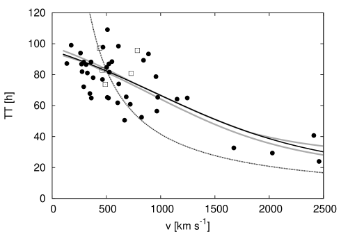
Figure 8: Transit times, $TT$, for CMEs near the central meridian. Filled circles and empty squares are observed $TT$s for CMEs in the region $-10\degr<$ CMD $<+10\degr$ in the learning sample and the validation sample, respectively. Solid black line represents $TT$s for CMD$=0\degr$ found by the best fit NN and solid grey lines are maximum and minimum values of $TT$s found by all 10 NN fits. The dotted line is a ’constant speed’ $TT$ function.

With filled circles and empty squares we show observed $TT$s in the region $-10\degr<$ CMD $<+10\degr$ for the learning and validation samples, respectively. Grey solid lines represent maximum and minimum values of all 10 NN fits as a function of initial CME velocity, $v$. The difference between these two extreme values is larger where there are fewer data points which is expected for NNs, as for any other fitting technique.

We can immediately see why the average error shown in Fig. 3 is fairly large ($\approx$ 12 h). For a smaller error the curve would have to follow every measured $TT$ more closely. However, such a curve would be unjustified from a statistical point of view and as a result the error of the validation sample would be significantly larger than the error of the learning sample. This occurs because NN can find a pattern in otherwise random variations between different events and is known as overfitting.

In the same graph we also show a ’constant speed’ model transit time, $TT=d/v$, with a dotted line, where we have taken distance from the Sun to the Earth to be $d=149.6\cdot$10⁶ km. Comparing this line with the one obtained with NN, we can see that CMEs slower than $v\approx$500 km s^-1 arrive sooner than predicted by the ’constant speed’ model. Converse is true for CMEs faster than $v\approx$500 km s^-1.

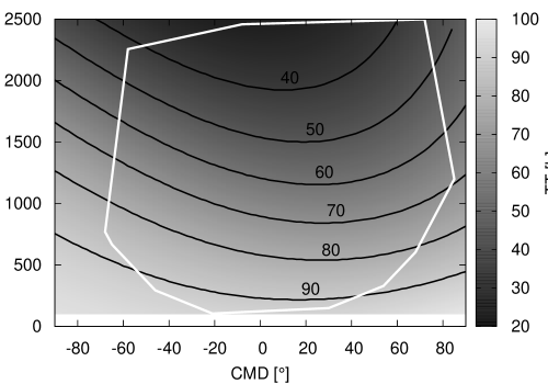
Figure 9: Map plot of $TT$ as function of $v$ and CMD. Solid lines are $TT$ isolines with values of $TT$ in hours for each isoline shown next to it. White solid line marks the smallest convex shape bounding all the events in our data set.

In Fig. 9 we show the calculated $TT$s from the best fit as a function of both input parameters, $v$ and CMD. Transit time isloines are shown as solid lines with values of $TT$ in hours indicated next to each isoline. Transit time, $TT$, is smaller for CMEs with larger velocities which was expected, but we can also see that $TT$s are smaller for positive CMDs (western solar hemisphere) in comparison with $TT$s for negative (eastern) CMDs.

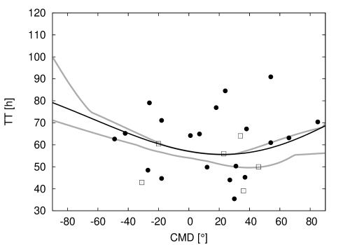
Figure 10: Transit times for CMEs with velocities between 1000 and 1500 km s^-1. Filled circles and empty squares are observed $TT$s for CMEs in the region 1000 km s${}^{-1}<L<$ 1500 km s^-1 from the learning sample and the validation sample, respectively. Solid black line are $TT$s for $v=1300$ km s^-1 found by the best fit NN and solid grey lines are maximum and minimum values of $TT$s found by all 10 NN fits.

In order to verify the dependence of $TT$ on CMD we take a closer look of this phenomenon in Fig. 10. We used the range between 1000 km s^-1 and 1500 km s^-1 for data points because this bin has a good CMD coverage and still a lot of data points (see Fig. 1). As in Fig. 8, solid circles are data points from the learning sample, while empty squares are events from the validation sample. Black solid line is the result of the best fit NN for $v=1300$ km s^-1 and grey lines are maximum and minimum values of all 10 NN fits as a function of CMD for the same speed. The distribution of data points in Fig. 10, assuming that it is not just an artefact of small number of events, is shifted westward which also illustrates the east-west asymmetry already observed in Fig. 9. As before, we can see the difference between maximum and minimum values growing very quickly in the regions with few or no data points.

Figure 11: Best fit curves found by NN for CMD$=+30\degr$ and CMD$=-30\degr$. The values of CMD parameters are given next to each curve.

In Fig. 11 we show the difference in calculated $TT$ as a function of CME initial speed, $v$, for CMD$=+30\degr$ and CMD$=-30\degr$. Calculated $TT$s for CMEs originating from the eastern hemisphere (negative CMD) are larger for almost all speeds, $v$, than $TT$s that NN predicts for their western counterparts.

5 Discussion and Conclusion

Arguably, the largest benefit of using NNs is that it is not necessary to specify the empirical function or hyper-surface that relates the input and output parameters. This becomes more difficult to determine as additional input parameters are included. Neural networks do not have such problems as long as proper statistical reasoning is used.

Here we have applied a NN to estimating ICME transit times using the LASCO CME speed and CMD source position from 153 events as input parameters. The average error of the whole sample for the best fit is 11.56 hours, which is comparable to other works (see Sect. 1 or Zhao & Dryer (2014)). Additional error of $\approx$1 hour can be expected due to the rounding of ICME arrival time to the nearest hour in most of the events in our dataset (Richardson & Cane, 2010). Looking at Figs. 8 and 10 it is clear that average errors can not be much smaller. Better results could be achieved with more input parameters to the NN. One parameter which almost certainly plays a significant part is the variable solar wind speed during CME transit through interplanetary space. We also know that energy released in the associated flare plays a role in early dynamics of CMEs (Vršnak, Sudar & Ruždjak, 2005) and it is quite possible that this effect is reflected in their actual $TT$ to Earth. In our case the number of data points at our disposal practically prohibits this approach. It is also possible to improve $TT$ prediction by tracking CMEs to larger distances, but this results in shorter lead times (Möstl et al., 2014).

The NN shown in this work only predicts when particular CME will reach 1 AU and it can’t be used to predict $TT$ to any other distance from the Sun. Therefore, it is only usable as a predictor for objects close to 1 AU, for example the Earth or STEREO satellites. It also does not predict whether the CME will actually hit the Earth or how geoeffective it will be.

The accuracy of CME TT forecasts is not significantly improved using the NN method discussed here. There is no way that one limited set of initial parameters can fit all the observed data much better than with $\approx$12 hour average error (Zhao & Dryer, 2014) at the present state of data quality and quantity. Case studies can offer better accuracy with a richer data set and by taking into account additional factors such as CME interactions (Lugaz et al., 2012; Temmer et al., 2012; Maričić et al., 2014) or variable solar wind (Temmer et al., 2011), but they usually depend on rare configurations of spacecrafts and the results of such analyses are usually too late to make any sort of real time predictions (Zhao & Dryer, 2014).

The results of NN shown in Fig. 8 are quite convincing that the CME is subjected to the drag force in the moving medium on its path through the interplanetary space. Vršnak & Žic (2007) already proposed a simple aerodynamic drag model for the CME dynamics. Moreover, in their Fig. 5, Vršnak & Žic (2007) show theoretical $TT$ curves which are very similar to our empirical one in Fig. 8. From the equation for the drag acceleration (Vršnak & Žic, 2007):

$$a=-\gamma(v_{CME}-w)|v_{CME}-w|,$$ (6)

where $w$ is the speed of the moving ambient medium we can easily interpret the intersect between the ’constant speed’ model, $a=0$, and the NN curve shown in Fig. 8. The intersect is actually the empirical value of the solar wind speed obtained by NN which for our analysis we can write with asymmetric error $w=505^{+7}_{-8}$ km s^-1.

Figs. 9, 10 and 11 show significant dependence of $TT$ on CMD. On average, CMEs originating on the western hemisphere (positive CMD) arrive sooner then their eastern hemisphere (negative CMD) counterparts. From Figs. 10 and 11 we can estimate that the difference is up to $\approx$10 hours. This result can be interpreted as a consequence of east-west deflection of CMEs. Another clue that deflection of CMEs is really happening can be found in our Fig. 1. The bounding surface containing all the events as well as their distribution in the parameter space is asymmetric and shifted westward. This means that CMEs on the eastern limb miss the Earth, while those on the western limb still have a chance to hit it. The same can be seen in the data published by Wang et al. (2004) who also noticed this westward shift of the Earth-bounding CME source regions.

From the isolines in Fig. 9 it is possible to infer how the CMD corresponding to the minimum $TT$ varies as a function of CME speed, $v$. While western CMDs were found for almost all speeds in the NN training runs made for this study, the locations were not stable such that even a qualitative assessment of the dependence of the CMD offset on $v$ is not advisable. The problem of the exact location of the $TT$ minimum is also visible in Fig. 10.

In a case study of a fast CME, Rollett et al. (2014) concluded that the CME evolves asymmetrically in exactly the same direction (eastward) as we can see in our results. In contrast to Wang et al. (2004), which propose that slow and fast CMEs are deflected in different direction, we see eastward deflection at all speeds. It is also not clear how the CH effect on CME trajectory (Gopalswamy et al., 2009; Lugaz et al., 2011) could account for any sort of statistical asymmetry in the east-west direction. Shen et al. (2011) proposed a model for latitudinal deflection of CMEs toward the solar equator, but it is not clear if their model could explain average longitudinal deflection that we see in our data.

References

- Alves, Echer & Gonzalez (2006) Alves M. V., Echer E., Gonzalez W. D., 2006, J. Geophys. Res. (Space Physics), 111, 7
- Boteler, Pirjola & Nevanlinna (1998) Boteler D. H., Pirjola R. J., Nevanlinna H., 1998, Advances in Space Research, 22, 17
- Cid et al. (2014) Cid C., Palacios J., Saiz E., Guerrero A., Cerrato Y., 2014, Journal of Space Weather and Space Climate, 4, A28
- Dierckxsens et al. (2015) Dierckxsens M., Tziotziou K., Dalla S., Patsou I., Marsh M. S., Crosby N. B., Malandraki O., Tsiropoula G., 2015, Sol. Phys., 290, 841
- Echer et al. (2008) Echer E., Gonzalez W. D., Tsurutani B. T., Gonzalez A. L. C., 2008, J. Geophys. Res. (Space Physics), 113, 5221
- Feynman & Gabriel (2000) Feynman J., Gabriel S. B., 2000, J. Geophys. Res., 105, 10543
- Fry et al. (2003) Fry C. D., Dryer M., Smith Z., Sun W., Deehr C. S., Akasofu S.-I., 2003, J. Geophys. Res. (Space Physics), 108, 1070
- Gopalswamy et al. (2001) Gopalswamy N., Lara A., Yashiro S., Kaiser M. L., Howard R. A., 2001, J. Geophys. Res., 106, 29207
- Gopalswamy et al. (2009) Gopalswamy N., Mäkelä P., Xie H., Akiyama S., Yashiro S., 2009, J. Geophys. Res. (Space Physics), 114, 0
- Gosling et al. (1990) Gosling J. T., Bame S. J., McComas D. J., Phillips J. L., 1990, Geophys. Res. Lett., 17, 901
- Gosling et al. (1991) Gosling J. T., McComas D. J., Phillips J. L., Bame S. J., 1991, J. Geophys. Res., 96, 7831
- Gosling et al. (1987) Gosling J. T., Thomsen M. F., Bame S. J., Zwickl R. D., 1987, J. Geophys. Res., 92, 12399
- Gui et al. (2011) Gui B., Shen C., Wang Y., Ye P., Liu J., Wang S., Zhao X., 2011, Sol. Phys., 271, 111
- Gurney (1997) Gurney K., 1997, An Introduction to Neural Networks. UCL Press, London, UK
- Li & Zhu (2013) Li R., Zhu J., 2013, Research in Astronomy and Astrophysics, 13, 1118
- Lugaz et al. (2011) Lugaz N., Downs C., Shibata K., Roussev I. I., Asai A., Gombosi T. I., 2011, ApJ, 738, 127
- Lugaz et al. (2012) Lugaz N., Farrugia C. J., Davies J. A., Möstl C., Davis C. J., Roussev I. I., Temmer M., 2012, ApJ, 759, 68
- Manoharan (2006) Manoharan P. K., 2006, Sol. Phys., 235, 345
- Maričić et al. (2014) Maričić D. et al., 2014, Sol. Phys., 289, 351
- Marubashi et al. (2015) Marubashi K., Akiyama S., Yashiro S., Gopalswamy N., Cho K.-S., Park Y.-D., 2015, Sol. Phys., 290, 1371
- Mays et al. (2015) Mays M. L. et al., 2015, Sol. Phys., 290, 1775
- Möstl et al. (2014) Möstl C. et al., 2014, ApJ, 787, 119
- Odstrcil, Riley & Zhao (2004) Odstrcil D., Riley P., Zhao X. P., 2004, J. Geophys. Res., 109, 2116
- Prša et al. (2008) Prša A., Guinan E. F., Devinney E. J., DeGeorge M., Bradstreet D. H., Giammarco J. M., Alcock C. R., Engle S. G., 2008, ApJ, 687, 542
- Richardson & Cane (2010) Richardson I. G., Cane H. V., 2010, Sol. Phys., 264, 189
- Richardson & Cane (2012) Richardson I. G., Cane H. V., 2012, Journal of Space Weather and Space Climate, 2, A1
- Richardson, Cliver & Cane (2001) Richardson I. G., Cliver E. W., Cane H. V., 2001, Geophys. Res. Lett, 28, 2569
- Rollett et al. (2014) Rollett T. et al., 2014, ApJL, 790, L6
- Schrijver & Mitchell (2013) Schrijver C. J., Mitchell S. D., 2013, Journal of Space Weather and Space Climate, 3, A19
- Schwenn et al. (2005) Schwenn R., Dal Lago A., Huttunen E., Gonzalez W. D., 2005, Annales Geophysicae, 23, 1033
- Shen et al. (2011) Shen C., Wang Y., Gui B., Ye P., Wang S., 2011, Sol. Phys., 269, 389
- Taktakishvili et al. (2009) Taktakishvili A., Kuznetsova M., MacNeice P., Hesse M., Rastätter L., Pulkkinen A., Chulaki A., Odstrcil D., 2009, Space Weather, 7, 3004
- Temmer et al. (2011) Temmer M., Rollett T., Möstl C., Veronig A. M., Vršnak B., Odstrčil D., 2011, ApJ, 743, 101
- Temmer et al. (2012) Temmer M. et al., 2012, ApJ, 749, 57
- Uwamahoro, McKinnell & Habarulema (2012) Uwamahoro J., McKinnell L. A., Habarulema J. B., 2012, Annales Geophysicae, 30, 963
- Valach et al. (2009) Valach F., Revallo M., Bochníček J., Hejda P., 2009, Space Weather, 7, 4004
- Vršnak et al. (2004) Vršnak B., Ruždjak D., Sudar D., Gopalswamy N., 2004, A&A, 423, 717
- Vršnak, Sudar & Ruždjak (2005) Vršnak B., Sudar D., Ruždjak D., 2005, A&A, 435, 1149
- Vršnak et al. (2014) Vršnak B. et al., 2014, ApJS, 213, 21
- Vršnak & Žic (2007) Vršnak B., Žic T., 2007, A&A, 472, 937
- Vršnak et al. (2013) Vršnak B. et al., 2013, Sol. Phys., 285, 295
- Wang et al. (2004) Wang Y., Shen C., Wang S., Ye P., 2004, Sol. Phys., 222, 329
- Wang et al. (2002) Wang Y. M., Ye P. Z., Wang S., Zhou G. P., Wang J. X., 2002, J. Geophys. Res. (Space Physics), 107, 1340
- Zhang et al. (2003) Zhang J., Dere K. P., Howard R. A., Bothmer V., 2003, ApJ, 582, 520
- Zhang et al. (2007) Zhang J. et al., 2007, J. Geophys. Res. (Space Physics), 112, 10102
- Zhao & Dryer (2014) Zhao X., Dryer M., 2014, Space Weather, 12, 448