Magnetic Field Strengths in Photodissociation Regions

Abstract

We measure carbon radio recombination line (RRL) emission at 5.3$\,{\rm GHz}$ toward four H ii regions with the Green Bank Telescope (GBT) to determine the magnetic field strength in the photodissociation region (PDR) that surrounds the ionized gas. Roshi (2007) suggests that the non-thermal line widths of carbon RRLs from PDRs are predominantly due to magneto-hydrodynamic (MHD) waves, thus allowing the magnetic field strength to be derived. We model the PDR with a simple geometry and perform the non-LTE radiative transfer of the carbon RRL emission to solve for the PDR physical properties. Using the PDR mass density from these models and the carbon RRL non-thermal line width we estimate total magnetic field strengths of $B\sim 100-300$ $\mu$G in W3 and NGC 6334A. Our results for W49 and NGC 6334D are less well constrained with total magnetic field strengths between $B\sim\ 200-1000$ $\mu$G. H i and OH Zeeman measurements of the line-of-sight magnetic field strength ($B_{\rm los}$), taken from the literature, are between a factor of $\sim 0.5-1$ of the lower bound of our carbon RRL magnetic field strength estimates. Since $|B_{\rm los}|\leq B$, our results are consistent with the magnetic origin of the non-thermal component of carbon RRL widths.

1 Introduction

Magnetic fields play an important role in many astrophysical objects including planets, stars, and galaxies (Parker, 1979). Measurements of magnetic fields in the cosmos, however, are difficult and therefore their paucity limits our ability to fully understand a wide range of astrophysical processes. For example, the role of magnetic fields in star formation is currently a hotly debated topic (see Crutcher, 2012, and references within). There are a handful of magnetic field diagnostics such as dust polarization, Faraday Rotation, and the Zeeman effect. Only the Zeeman effect can directly measure the line-of-sight magnetic field strength in interstellar clouds (Crutcher, 2012).

Observations of spectral lines from molecular, neutral, and ionized gas indicate line widths that are broader than the thermal width, even on small spatial scales where macroscopic effects such as rotation would be minimal. These non-thermal line widths are thought to be a result of motions either from MHD waves (e.g., Mouschovias, 1975) or turbulence (e.g., Morris et al., 1974). Specific examples include CO in molecular clouds (Arons & Max, 1975) and H$\alpha$ in H ii regions (Ferland, 2001; Beckman & Rela$\tilde{\rm n}$o, 2004). H₂CO absorption toward compact extragalactic sources reveals secular changes to the absorption intensity on AU scales, with a non-thermal component to the velocity dispersion, indicating that these motions occur on very small spatial scales (Marscher, et al., 1993).

Carbon radio recombination line (RRL) emission detected toward star formation complexes originates from the cooler, mostly neutral gas, surrounding the H ii region called the photodissociation region (PDR). Roshi (2007) suggested that the non-thermal line widths of carbon RRLs toward PDRs adjacent to H ii regions are dominated by MHD waves and could be used to derive the magnetic field strength. The PDR is a thin layer lying between the molecular cloud and the H ii region. At cm-wavelengths the carbon RRL intensity is enhanced by stimulated emission from the background H ii region (Roshi et al., 2005; Quireza et al., 2006). This provides information about the geometry and allows for relatively simple PDR models to be developed (see Roshi et al., 2005). Here we test the Roshi (2007) hypothesis by measuring the non-thermal line widths in four PDRs that also have either H i or OH Zeeman based determinations of magnetic field strength.

2 Observations and Data Reduction

We observed the RRL and continuum emission at C-band (4-6$\,{\rm GHz}$) toward four H ii regions with the National Radio Astronomy Observatory (NRAO) Green Bank Telescope (GBT) on 5 April, 27 April, and 8 May 2008. The GBT has a half-power beam-width (HPBW) of $2\hbox to0.0pt{.\hss}{{}^{\prime}}34$ at an observing frequency of 5.3$\,{\rm GHz}$. The aperture efficiency and beam efficiency are 0.70 and 0.92, respectively, yielding a sensitivity of 2 K/Jy. We selected W3, W49, NGC 6334A, and NGC 6334D as targets since these sources have bright carbon RRL emission regions and Zeeman measurements in the neutral gas. Moreover, these sources have been detected in carbon RRLs with a similar spatial resolution but at a different frequency (8.7 GHz) with the NRAO 140 Foot telescope (Quireza et al., 2006). We require at least two carbon RRLs, separated in frequency, to model the PDR and derive the magnetic field strength (see §4). The ${\rm C}91\alpha$ and ${\rm C}92\alpha$ RRLs were observed with the 140 Foot. At these frequencies the 140 Foot has a HPBW of $3\hbox to0.0pt{.\hss}{{}^{\prime}}20$. The aperture efficiency and beam efficiency are 0.51 and 0.68, respectively, giving 0.27 K/Jy.

For each GBT observing session we first checked the pointing and focus by observing a nearby calibrator. Continuum scans in R.A. and Decl. were then made to measure the free-free emission. We scanned the GBT both forward and backward for each cardinal direction while simultaneously sampling both linear, orthogonal polarizations. So each continuum observation consisted of 4 scans times 2 polarizations or 8 total measurements. We used the Digital Continuum Receiver (DCR) with a bandwidth of 80$\,{\rm MHz}$, centered at 5.3$\,{\rm GHz}$, and an integration time of 0.1 s. The GBT was driven at a rate of 80 arcsec per second for 30 s, providing a scan length of 40 arcmin. Data from both directions (forward and backward) and linear polarizations (XX and YY) were averaged for several continuum observations to increase the signal-to-noise ratio of the continuum intensity measurement.

Finally, spectra were taken using total power, position switching where we observed a reference (OFF) position for 6 minutes, and then, tracking the same sky path, observed the target (ON) position for 6 minutes. The Autocorrelator Spectrometer (ACS) was configured with 8 spectral windows, each with two orthogonal, linear polarizations yielding 16 independent spectra. Each spectral window contained 4096 channels with a bandwidth of 12.5$\,{\rm MHz}$, providing a spectral resolution of 3.05$\,{\rm kHz}$, or 0.18$\,{\rm km\,s^{-1}}$ per channel at 5$\,{\rm GHz}$. We centered each spectral window to include the carbon RRLs: ${\rm C}104\alpha$-${\rm C}110\alpha$, and ${\rm C}112\alpha$. The ${\rm C}111\alpha$ transition is confused by a higher order RRL and therefore was not observed. The intensity scale was calibrated in Kelvins using noise diodes that injected noise into the signal path. We verified that the accuracy of the calibration was within 10% by making continuum observations toward 3C286.

Both the spectral line and continuum data were reduced and analyzed with the single-dish software package TMBIDL. Typically, a third-order polynomial function was fit to the continuum baseline and removed from the data. A Gaussian profile was fit to the main continuum source to determine the peak intensity, full-width at half-maximum (FWHM) H ii region size, and the center position. Spectral line data were reduced by first averaging spectra in each spectral window, and then combining the different Cn$\alpha$ transitions to improve the signal-to-noise ratio. At these high principal quantum numbers the difference in energy between adjacent Cn$\alpha$ transitions is negligible and therefore we can average these different transitions (e.g., Balser, 2006). This was done by first resampling the spectral channels of each spectral window to match the velocity resolution of the 104$\alpha$ spectral window and then shifting each spectrum to be at the same LSR velocity. Here no correction was made for the different HPBW’s. The ${\rm C}112\alpha$ RRL was not included in the average, however, because of variations in the calibration scale near the carbon RRL that we suspect was caused by resonances in the telescope feed. A third-order polynomial was fit to the line-free regions of the spectral baseline to remove the continuum level and any other instrumental baseline structure. Multiple Gaussian functions were then fit to the various RRLs within each spectral window to determine the peak line intensity, the FWHM line width, and the LSR velocity. The He and heavier element RRLs were fit simultaneously, whereas the H RRL was fit separately.

3 Radio Continuum and RRL Results

Star forming complexes that contain early-type stars consist of H ii regions that have formed due to the large number of hydrogen-ionizing photons, molecular clouds where the next generation of stars may form, and PDRs that lie at their interface. The radio continuum emission observed toward star forming complexes is primarily produced from free-free emission in the H ii region. The non-thermal Galactic background emission may contribute to the observed continuum, but because this background emission is smoothly distributed over spatial scales larger than the H ii region size it will be removed in our baseline fitting procedures. Figures 1-2 show the continuum profiles for both the R.A. and Decl. scans. Table 1 summarizes the H ii region continuum parameters based on Gaussian fits to the main source component. Listed are the source name, the B1950 equatorial coordinates, the distance from the Sun, $R_{\rm Sun}$, and the peak intensity, $T_{\rm C}$, and FWHM size, $\Theta$, and their associated $1\sigma$ errors.

We detect hydrogen and helium RRL emission from the four H ii regions in our sample. Typically RRLs from heavier elements are not detected from H ii regions since they have small abundances producing line intensities below the sensitivity limit of most radio telescopes. In many cases, however, a narrower, weaker line is detected at higher frequencies and has been identified as carbon RRL emission formed within the PDR (e.g., see Zuckerman & Palmer, 1968; Wenger et al., 2013). The physical temperature of PDRs is about an order of magnitude lower than that in H ii regions. This lower temperature makes the carbon RRL from PDRs detectable since the line optical depth has a strong inverse dependence on the gas temperature. Since the carbon RRL arises from the PDR it often has a slightly different LSR velocity than the hydrogen and helium RRLs. Figure  3 shows spectra for each source with a magnified view to highlight the carbon profiles. The velocity scale is defined relative to the hydrogen RRL which resides about 150$\,{\rm km\,s^{-1}}$ at more positive velocities. Each spectrum reveals multiple heavy element RRL profiles. Carbon is likely to be the brightest heavy element RRL because of its low ionization potential (11.3 ev), high cosmic abundance, and low depletion. Other candidates are sulfur and magnesium. The W49 spectrum contains two carbon RRLs that have been shown to originate from spatially distinct PDRs (Roshi et al., 2006). For each source there exists a weaker transition, labeled as “X”, that is consistent with an element heavier than carbon since the line center is at higher frequencies. For W3 and W49 the “X” line may be another carbon RRL from a different component, or possibly sulfur. Based on the center velocity and reduced line intensity we expect the “X” line to be sulfur in the two NGC 6334 sources. Table 2 summarizes the RRL line parameters. Listed are the source name, the element, the peak intensity, $T_{\rm L}$, the FWHM line width, $\Delta{V}$, the LSR velocity, $V_{\rm LSR}$, the total integration time, $t_{\rm integ}$, and root-mean-square noise in the line-free region, rms, together with their $1\,\sigma$ errors.

4 Photodissociation Region Models

To derive the total magnetic field strength requires knowing both the carbon RRL non-thermal velocity width and the PDR density (see §5). Here we develop PDR models to determine the PDR density that are constrained by carbon RRLs at two different frequencies (see, e.g., Roshi et al., 2005). Infrared observations of H ii region/PDR/molecular cloud complexes typically find $22\,\mu m$ emission surrounded by $12\,\mu m$ emission (e.g., see Anderson et al., 2014). The $22\,\mu m$ emission is produced by stochastically heated small dust grains within the H ii region, whereas the $12\,\mu m$ emission is thought to be polycyclic aromatic hydrocarbon, PAH, emission within the PDR. We therefore consider a simplified model consisting of homogeneous cylinders of PDR material, co-located with the molecular gas, in front of the H ii region. This geometry is consistent with both observations and models. Observations show that the carbon RRL intensity is correlated with the H ii region continuum intensity (e.g., Quireza et al., 2006). This implies that the carbon RRL is amplified by stimulated emission from the H ii region which lies behind the PDR. Models of the radiative transfer show that without stimulated emission, at cm-wavelengths, we would not have the sensitivity to detect the carbon RRL emission (Roshi et al., 2005).

We use the formulation of Shaver (1975) to perform the radiative transfer and to calculate the carbon RRL brightness temperature at frequency $\nu$:

$$T_{\rm L}^{\rm B}(\nu) = T_{\rm bg}(\nu)e^{-\tau_{C}(\nu)}(e^{-\tau_{\rm L}(\nu)}-1)+$$ (1)

$$T_{\rm PDR}\left(\frac{b_{\rm m}\tau_{\rm L}(\nu)^{*}+\tau_{\rm C}(\nu)}{\tau_{\rm L}(\nu)+\tau_{\rm C}(\nu)}(1-e^{-(\tau_{\rm L}(\nu)+\tau_{\rm C}(\nu))})-(1-e^{-\tau_{\rm C}(\nu)})\right),$$

where the first term is the contribution to the line temperature due to the background radiation field and the second term is the intrinsic emission from the PDR cylinder. The background temperature, $T_{\rm bg}(\nu)$, is dominated by the H ii region and so

$$T_{\rm bg}(\nu)=T_{\rm e}(1-e^{-\tau_{\rm C}^{HII}(\nu)}),$$ (2)

where $\tau_{C}^{HII}(\nu)$ is the H ii region continuum optical depth given by Equation (31) in Shaver (1975). The PDR thermal temperature, $T_{\rm PDR}$, is typically between $100-500$$\,{\rm K}$ (e.g., Abel et al., 2005). The line and continuum optical depths of the PDR are given by $\tau_{\rm L}(\nu)$ and $\tau_{\rm C}(\nu)$, respectively. We calculate the PDR continuum opacity from Equation (31) in Shaver (1975).

The PDR line opacity is:

$$\tau_{\rm L}(\nu)=b_{\rm n}\beta_{\rm n}\tau_{\rm L}(\nu)^{*},$$ (3)

where $b_{\rm n}$ and $\beta_{\rm n}$ are the departure coefficients of the energy level $\rm{n}$. The LTE line opacity $\tau_{\rm L}(\nu)^{*}\propto(n_{\rm e}^{\rm PDR}\,n_{\rm i}^{\rm PDR}\,\ell$) where $n_{\rm e}^{\rm PDR}$ and $n_{\rm i}^{\rm PDR}$ are the electron and ion number densities of the PDR, respectively, and $\ell$ is the PDR cylinder thickness (see Equation 71 in Shaver, 1975). We assume all of the ions in the PDR arise from carbon and therefore $n_{\rm i}^{\rm PDR}=n_{\rm C^{+}}^{\rm PDR}=n_{\rm e}^{\rm PDR}$. The departure coefficients are calculated using a new computer code developed by Roshi et al. (2014) that includes modification of the level population of the carbon atom due to a dielectronic-like recombination process (Walmsley & Watson, 1982) and a background radiation field from an H ii region. This is a modified version of the original code developed by Brocklehurst & Salem (1977) and Walmsley & Watson (1982). For the computation of $b_{\rm n}$ and $\beta_{\rm n}$, we assume 25% of the carbon atoms are depleted onto dust grains (Natta et al., 1994), and a cosmic carbon abundance of C/H = $3.9\times 10^{-4}$ by number (Morton, 1974). With these assumptions the hydrogen number density in the PDR is $n_{\rm H}=3.4\times 10^{3}\,n_{\rm e}$.

The PDR models require the background, H ii region, intensity as a function of frequency to be known, for calculating the departure coefficients. We adopt the spherical, homogeneous H ii region models of Balser et al. (1995) and constrain these models with our C-band (5.3$\,{\rm GHz}$) radio continuum data, listed in Table 1, to derive the size, $\theta_{\rm sph}$, electron number density, $n_{\rm e}$, and the number of hydrogen-ionizing photons emitted per second, $N_{\rm L}$. The values of $N_{\rm L}$ provide an estimate of the stellar spectral type, assuming all of the hydrogen-ionizing photons come from a single star. The peak emission measure, $EM=\int{n_{\rm e}d\ell}$, is taken from the formalism of Wood & Churchwell (1989). Radio continuum data alone cannot constrain the electron temperature ($T_{\rm e}$), and therefore we adopt the values from Balser et al. (1999) that were derived from RRL and continuum emission at 8.7$\,{\rm GHz}$. Table 3 lists these physical properties for each H ii region in our sample.

We use the numerical code developed by Roshi et al. (2014) to compute the carbon RRL flux density from the PDR by solving the non-LTE radiative transfer equation. The line temperature, $T_{\rm L}$, provided by the model is converted to flux density, $S_{\rm L}$, using the equation

$$S_{\rm L}=\frac{2\,k\,T_{\rm L}}{\lambda^{2}}\,\Omega$$ (4)

where $k$ is the Boltzmann constant, $\lambda$ is the observed wavelength, and $\Omega$ is the source solid angle. We assume the source size equals the GBT’s HPBW of $2\hbox to0.0pt{.\hss}{{}^{\prime}}34$. There are three free parameters in this model: the PDR temperature, $T_{\rm PDR}$, the PDR electron number density, $n_{\rm e}^{\rm PDR}$, and the PDR cylinder thickness, $\ell$. Since PDR temperatures range from 100-500$\,{\rm K}$, we consider values of 100$\,{\rm K}$, 200$\,{\rm K}$, and 500$\,{\rm K}$ for our models. The departure coefficients are a function of $T_{\rm PDR}$ and $n_{\rm e}^{\rm PDR}$. They are calculated for a set of electron densities between 1 and 500$\,{\rm cm^{-3}}$ for each $T_{\rm PDR}$ value. Modeling requires two observed carbon RRL intensities to solve for $n_{\rm e}^{\rm PDR}$ and $\ell$, since we assume a set of values for the PDR gas temperatures. Therefore, we use the 140 Foot 8.7$\,{\rm GHz}$ carbon RRL data from Quireza et al. (2006) together with the GBT 5.3$\,{\rm GHz}$ observations discussed in §2. Antenna temperatures are converted to flux density by using 2 K/Jy and 0.27 K/Jy for the GBT and 140 Foot, respectively. We assume the PDR is filling the $2\hbox to0.0pt{.\hss}{{}^{\prime}}34$ HPBW of the GBT and we therefore scale the 140 Foot flux density by the ratio of the beam areas, $(2\hbox to0.0pt{.\hss}{{}^{\prime}}34/3\hbox to0.0pt{.\hss}{{}^{\prime}}20)^{2}$. Table 4 summarizes the constraints to the models. Listed are the source name, the RRL transitions, the peak intensity, the FWHM line width, the LSR velocity, and the flux density, together with their associated errors. The errors listed for the carbon RRL peak intensity, FWHM line width, and LSR velocity are the $1\sigma$ uncertainties in the Gaussian fits to the line profile. These errors are propagated to the flux density, $S_{\nu}$.

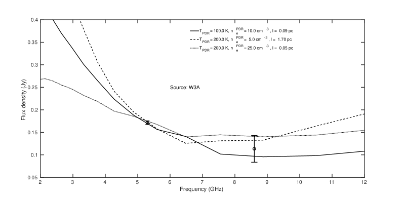
Figure 4: PDR model results for W3. The flux density is plotted as a function of frequency. The lines correspond to different models and the points are from carbon RRL observations at 5.3$\,{\rm GHz}$ (§2) and 8.7$\,{\rm GHz}$ (Quireza et al., 2006). The error bars shown are $\pm\ 3\sigma$ values.

For each PDR temperature we ran a grid of models with a set of PDR electron densities, and then solved for the PDR cylinder thickness. So for each ($T_{\rm PDR}$, $n_{\rm e}^{\rm PDR}$) pair choice, $\ell$ was varied to determine, by eye, the range of $\ell$ that was consistent to with our two observational data points within the errors. Therefore for each PDR temperature we determined a range of possible values for $n_{\rm e}^{\rm PDR}$ and $\ell$. We explored $n_{\rm e}^{\rm PDR}$ = 1, 5, 10, 25, and 50$\,{\rm cm^{-3}}$ for W3 and NGC 6334A; and $n_{\rm e}^{\rm PDR}$ = 5, 10, 25, 50, 100, and 200$\,{\rm cm^{-3}}$ for W49 and NGC 6334D. Model results are shown in Figures 4 through 7 where we plot the flux density as a function of frequency. The curves correspond to the models that set the extreme range in $n_{\rm e}^{\rm PDR}$ and $\ell$ for each PDR temperature, whereas the points are the constraints from the GBT and 140 Foot observations. For NGC 6334A, only one model in our grid is consistent with the data to within the uncertainties. Our modeling predicts lower PDR temperatures ($\lesssim 200$) for W3 and NGC 6334A. The flux density uncertainties are significantly higher for the 140 Foot X-band data and therefore dominate the scatter in these plots. The results are summarized in Table 5. For each PDR temperature we show the range of $n_{\rm e}^{\rm PDR}$ and $\ell$ values that “fit” the data; that is, their model curves lie within the observed error bars. Listed in Table 5 are the source name, the PDR temperature, the range of PDR electron densities, the range of cylinder thicknesses, and the range of magnetic field strengths (see below).

5 Magnetic Field Strength

It is now well established that the observed spectral line widths from molecular clouds are significantly larger than expected from thermal broadening alone. Arons & Max (1975) first proposed that this non-thermal line width is due to MHD waves, but the contribution of a pure hydrodynamic turbulence component cannot be ruled out (Morris et al., 1974). Spectral line widths from PDRs, which reside at the interface between the molecular cloud and the H ii region, are also dominated by non-thermal broadening. Roshi (2007) investigated the origin of this non-thermal component in PDRs using carbon RRLs. He concluded that (1) the origin of the non-thermal carbon RRL width is magnetic; (2) the non-thermal line width is approximately the Alf$\acute{v}$en speed in the PDR; and (3) the minimum MHD wavelength for which carbon ions and neutrals are strongly coupled is much smaller than the size of the PDR.

Perturbations in the magnetic field due to MHD waves create a velocity field in the plasma. This velocity field results in the non-thermal broadening of the observed spectral lines. The amplitude of the velocity field will be equal to the Alf$\acute{v}$en speed if the perturbing magnetic field is approximately equal to the total magnetic field strength, B. But pure hydrodynamic motions in the PDR may also contribute to the non-thermal width of spectra lines. We therefore introduce a parameter $\alpha$ to relate the Alf$\acute{v}$en speed, $V_{\rm A}$ and the observed non-thermal width of the spectral line:

$$V_{\rm A}=\alpha\frac{\Delta{V_{\rm nt}}}{\sqrt{8ln(2)}},$$ (5)

where $\Delta{V_{\rm nt}}$ is the FWHM non-thermal line width defined as

$$\Delta{V_{\rm nt}}=\sqrt{\Delta{V}^{2}-\Delta{V_{\rm t}}^{2}}.$$ (6)

Here $\Delta{V}$ is the observed FWHM line width and $\Delta{V_{\rm t}}$ is the thermally broadened FWHM line width given by

$$\Delta{V_{\rm t}}=\bigg{[}4\,ln(2)\bigg{(}\frac{2kT_{\rm PDR}}{m_{\rm c}}\bigg{)}\bigg{]}^{1/2},$$ (7)

where $m_{\rm c}$ is the mass of the carbon atom (Shaver, 1975, Equation 57). At one extreme, $\alpha\sim 0$ if the turbulence is non-magnetic in origin. At the other extreme, where the magnetic field dominates the turbulent motions, $\alpha\leq\sqrt{3}$. The exact value depends on the geometry of the magnetic and matter perturbations in the PDR since we need to convert the observed, one dimensional velocity dispersion into a three dimensional velocity dispersion (see for example McKee & Zweibel, 1995). The parameter $\alpha$ must be determined by observations. Roshi (2007) compared the magnetic field strength measured via the Zeeman effect in molecular clouds with the magnetic field strength derived from carbon RRLs in PDRs (see Roshi’s Figure 3). Such a comparison is possible since it has been shown that the magnetic field strength scales with density (Crutcher, 1999). From this comparison Roshi (2007) concluded that the non-thermal motions in PDRs are primarily caused by MHD waves and that $\alpha\sim 1$. Here we follow Roshi et al. (2014) and take $\alpha=\sqrt{3}/2=0.87$ as a mean value between the two extremes, mentioned above.

The magnetic field is given by

$$B=V_{\rm A}\sqrt{4\pi\,\rho},$$ (8)

where $\rho$ is the mass density of the gas coupled to the magnetic field (Parker, 1979). Roshi (2007) showed that the size of the PDR is larger than the minimum MHD wavelength. Thus in the PDR there exists a spectrum of MHD waves for which carbon ions and neutrals are strongly coupled to the field. The perturbations produced by these waves result in the non-thermal broadening of carbon lines. The ions and neutrals are coupled to these waves which implies that $\rho$ in Equation 8 should be the total (i.e., ion, atomic, and molecular) mass density of the PDR. The PDR mass density is given by

$$\rho=n_{\rm H}\,\mu\,m_{\rm H},$$ (9)

where $n_{\rm H}$ is the hydrogen number density, $m_{\rm H}$ is the hydrogen mass, and $\mu$ is the mean molecular weight. The hydrogen number density is determined by modeling the observed carbon lines. A pure hydrogen and helium gas with a He/H ratio of 10% by number yields $\mu=1.4$. Since the contribution of heavier elements, such as carbon, to the mean molecular weight is negligible, we take $\mu=1.4$.

In Table 5 we list a range of magnetic field strengths calculated using Equation 8 and the range of determined $n_{\rm e}^{\rm PDR}$ values for each PDR temperature. Most of the uncertainty in determining $B$ comes from our PDR models and therefore we specify a range of possible values instead of a value and $1\,\sigma$ error. The exception is NGC 6334A where only one model fits the data. The magnetic field strength for W49 and NGC 6334D are not well constrained with a wide range of possible magnetic field strengths. N.B., these uncertainties do not include any contribution to $\alpha$ which can range from 0 to $\sqrt{3}$.

6 Discussion

The role of magnetic fields in star formation has been an important astrophysical topic for decades (Shu et al., 1987; McKee & Ostriker, 2007). Recently, the debate has centered around competing theories that depend on the strength of the magnetic field. Strong magnetic fields will support molecular clouds from collapse, but neutral material will slip past these fields and thereby increase the molecular mass in a process called ambipolar diffusion (Shu et al., 1987). On the other hand, weak magnetic fields allow molecular clouds to form from turbulent flows on time scales equal to the free fall time (MacLow & Klessen, 2004). There are also star formation theories that include both of these processes (e.g., Nakamura & Li, 2005). Understanding magnetic field properties in star forming complexes provides important constraints to these theories (Crutcher, 2012).

Measuring magnetic field properties in star forming complexes is difficult, however, and therefore additional data are necessary to properly constrain star formation models. Roshi (2007) proposed a new method of deriving the magnetic field strength in PDRs using carbon RRLs. If the non-thermal motions in PDRs are dominated by MHD waves, then the non-thermal line widths provide a measure of the magnetic field strength. Here we test this hypothesis by comparing the magnetic field strength derived from carbon RRLs with Zeeman measurements in four sources: W3, W49, NGC 6334A and NGC 6334D. Zeeman observations provide a measure of the magnetic field along the line-of-sight (LOS) and therefore information on the morphology and a lower limit to the magnetic field strength (i.e., $|B_{\rm los}|\leq\ B$). If we consider a large number of PDRs that have a magnetic field that is oriented randomly relative to the LOS, then statistically $B=2\,|B_{\rm los}|$ (Crutcher, 1999). The magnetic field orientations in PDRs may not be random, however, given their geometry and formation.

Below we discuss each source separately.

W3 is a nearby, bright H ii region with at least 8 resolved components (A-H) in the core region (see, e.g., Tieftrunk et al., 1997). Roberts et al. (1993) derived the LOS magnetic field strength from H i Zeeman observations to be $B_{\rm los}=-47\pm\ 3$ $\mu$G, $+103\pm\ 7$ $\mu$G, and $+36\pm\ 6$ $\mu$G toward components A, B, and C+D, respectively. Our GBT observations are centered near W3A but include most of the core. We therefore consider $|B_{\rm los}|=30-110$ $\mu$G for comparison with our GBT data. The LSR velocity of the carbon RRL is $-39.1$$\,{\rm km\,s^{-1}}$, consistent with the H i Zeeman data. We estimate $B$ to be between $140-320$ $\mu$G.

W49 is one of the most luminous star forming complexes in the Galaxy and contains the H ii region W49A and a supernova remnant W49B (De Pree et al., 1997). Our GBT observations cover the W49A north region that consists of a ring of ultracompact H ii regions. Brogan & Troland (2001) detected the H i Zeeman line toward W49A and determined $|B_{\rm los}|=60-300$ $\mu$G. The $V_{\rm LSR}\sim 4$$\,{\rm km\,s^{-1}}$ $B_{\rm los}$ component is negative, whereas the $V_{\rm LSR}\sim 7$$\,{\rm km\,s^{-1}}$ $B_{\rm los}$ component is positive. Also, higher resolution Zeeman detections are stronger. Our GBT data constrain the magnetic field strength to be between $B=200-1300$ $\mu$G. Our C-band data contain two velocity components ($\sim 14$$\,{\rm km\,s^{-1}}$ and $\sim 4$$\,{\rm km\,s^{-1}}$), but the lower spectral resolution 140 Foot, X-band data has only one component at $\sim 7$$\,{\rm km\,s^{-1}}$. We have modeled the PDR using the C-band $\sim 14$$\,{\rm km\,s^{-1}}$ component. The results are similar if we use the $\sim 4$$\,{\rm km\,s^{-1}}$ component.

Since W49 is complex and distant ($R_{\rm Sun}=11.8$$\,{\rm kpc}$), it is difficult to compare the VLA Zeeman observations with our lower resolution GBT data. The carbon RRL emission regions may not be probing the same volume of gas as the VLA H i data. The differences in LSR velocity between our C-band and X-band carbon RRL data are troubling and therefore our results for W49 are suspect. Furthermore, the carbon RRL intensity is weighted by the emission measure ($\propto n_{\rm e}^{2}$), whereas the H i intensity is proportional to the hydrogen column density. So the carbon RRLs may be probing denser gas where the magnetic field strengths should be higher.

NGC 6334 is a nearby ($R_{\rm Sun}=1.7$$\,{\rm kpc}$), star forming region that contains at least seven star forming components (Kraemer et al., 2000). Here we focus on components A and D. Sarma et al. (2000) made H i and OH VLA measurements toward both of these components with LSR velocities around $-2$$\,{\rm km\,s^{-1}}$ to $-5$$\,{\rm km\,s^{-1}}$, consistent with our carbon RRL velocities. Significant Zeeman detections were made toward NGC 6334A in OH where $B_{\rm los}=148\pm\ 20$ $\mu$G and $B_{\rm los}=162\pm\ 33$ $\mu$G for the 1665$\,{\rm MHz}$ and 1667$\,{\rm MHz}$ lines. We consider $|B_{\rm los}|=128-195$ $\mu$G for comparison with GBT data. From our carbon RRLs we estimate $B=190\pm\ 96$ $\mu$G, where we assume a 50% error. For NGC 6334D, Sarma et al. (2000) measure $B_{\rm los}=-93\pm\ 13$ $\mu$G from H i Zeeman spectra yielding $|B_{\rm los}|=80-106$. Our carbon RRL data toward NGC 6334D do not provide a good constraint for the magnetic field with $B=180-1200$ $\mu$G, but the lower bound is within a factor of two relative to the Zeeman value.

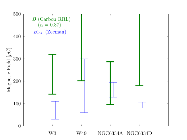
Figure 8: Magnetic field strengths derived here from carbon RRLs (thick green lines) for W3, W49, NGC 6334A, and NGC 6334D, compared to line-of-sight magnetic field strengths from Zeeman observations (blue lines). The magnetic field strengths from carbon RRLs correspond to the range of values in our model grid that are consistent with the data. The range for $|B_{los}|$ are taken from H i or OH Zeeman measurements in the literature (see text). The plot has been truncated at $B=500\,\mu G$ for clarity.

Figure 8 summarizes these results. We plot a comparison of the magnetic field strength from our carbon RRL measurements with the LOS magnetic field strength from Zeeman spectra as discussed above. We assume a 50% error for NGC 6334A since we were not able to determine a range of $B$ values from our models. The uncertainties are quite large but the trend is that $|B_{\rm los}|$ is between $0.5-1.0$ of the lower bound of $B$, and this is consistent with our expectations that $|B_{\rm los}|\leq\ B$. Similar results are obtained for PDRs in OrionB (Roshi et al., 2014) and W3, W49, and S88B (Roshi, 2007).

Overall, our GBT carbon RRL data are consistent with the hypothesis of Roshi (2007) that the non-thermal motions in PDRs have a magnetic origin. But our results are not conclusive since we do not know $\alpha$ or the orientation of the magnetic field vector. Moreover, there are many assumptions and approximations in deriving the magnetic field strength using the carbon RRL method. Here we list some of the issues.

1. PDR Geometry: We assume the PDR region is a thin cylinder that covers the H ii region. Infrared data do show that PDR material as seen in 8$\,\mu{\rm m}$ emission typically surrounds H ii regions (24$\,\mu{\rm m}$ emission) with a thin, sheet-like morphology (e.g., Anderson et al., 2014). Our GBT and 140 Foot data lack the spatial resolution, however, to confirm that the PDR covers the H ii region. Interferometers like the VLA can spatially resolve some of these regions with enough sensitivity to verify this geometry (see Roshi et al., 2014).

2. Model Constraints: Observations at only two frequencies are used to constrain three free parameters: $T_{\rm PDR}$, $n_{\rm e}^{\rm PDR}$, and $\ell$. Therefore we had to assume several values for the PDR temperature to constrain the fits. This could be significantly improved by obtaining additional carbon RRL data separated in frequency.

3. H i/OH Zeeman Data: We use H i and OH Zeeman data to check the hypothesis by Roshi (2007) that carbon RRL non-thermal widths are magnetic in origin with the goal of using such data to determine magnetic field strengths in PDRs. We expect the H i and OH emission to arise from the PDR but this emission may not be sampling the same region as the carbon RRL emission. RRLs probe higher density gas compared with H i, and our models indicate that cm-wavelength carbon RRLs are sensitive to PDR material in front of the H ii region relative to our line-of-sight. So we may not be sampling the same material. This can be mitigated by observing the carbon RRL Zeeman effect.

4. Alf$\acute{\it v}$en Speed: We calculate $V_{\rm A}$ from $\Delta{V_{\rm nt}}$. If the gas pressure is small compared to the magnetic pressure then the velocity dispersion should be approximately the Alf$\acute{v}$en speed (see Arons & Max, 1975). But we have to convert the one-dimensional velocity dispersion, $\Delta{V_{\rm nt}}$, to a three-dimensional velocity dispersion. Since we do not know the magnetic field geometry the value of $\alpha$ must be constrained from observations. Therefore, the parameter $\alpha$ in Equation 5 is another free parameter. The magnetic field strength is proportional to $\alpha$, and here we assume $\alpha=\sqrt{3}/2$. The uncertainties given in Table 5 are taken from the PDR models and do not include the uncertainties in $\alpha$.

5. B versus B_los: Since Zeeman observations probe the LOS magnetic field strength we cannot directly compare these results with our estimates of the total magnetic field strength from our carbon RRL data for a given source. If we observed many PDRs using both methods we could make a statistical argument that $B=2\,|B_{\rm los}|$ (e.g., Crutcher, 1999). But this assumes that the orientation of the magnetic field vector is random which may not be true for PDRs.

How to proceed? Observations of carbon RRLs at several different frequencies using both the VLA and GBT could significantly improve our understanding of the PDR geometry and provide better constraints to the models. Observing many sources would allow a statistical comparison with Zeeman results and an estimate of $\alpha$. A more direct comparison of the magnetic field strength could be made by measuring the Zeeman effect in carbon RRLs. To do this in many sources with good accuracy, however, would probably require the SKA or NGVLA. Nevertheless, our results here are consistent with the Roshi (2007) hypothesis of a magnetic origin for the observed carbon RRL non-thermal line widths.

7 Summary

Magnetic fields play an important role in star formation, but they are difficult to measure, and therefore have not provided very stringent constraints on a host of relevant astrophysical processes. Roshi (2007) proposed a new technique to derive magnetic field strengths using carbon RRLs in PDRs. It assumes that the non-thermal motions in PDRs are dominated by MHD waves. Here we measure the ${\rm C}104\alpha$-${\rm C}110\alpha$ (5.3$\,{\rm GHz}$) RRL emission with the GBT toward four star forming regions to test this hypothesis. We use the models developed by Roshi et al. (2014) to calculate the carbon RRL flux density by performing the non-LTE radiative transfer. To constrain these models requires at least two carbon RRLs separated in frequency, and to do this we use the ${\rm C}91\alpha$-${\rm C}92\alpha$ (8.7$\,{\rm GHz}$) RRLs from Quireza et al. (2006) together with the observations reported here.

We estimate $B\sim 100-300$ $\mu$G in W3 and NGC 6334A, and $B\sim 200-1000$ $\mu$G in W49 and NGC 6334D. These results are consistent with H i and OH Zeeman observations, which measure the line-of-sight magnetic field strength $B_{\rm los}$. That we find $|B_{\rm los}|\leq\ B$ in all cases is consistent with the hypothesis that the non-thermal component of the velocity dispersion measured by carbon RRLs in magnetic in origin. There are many assumptions and approximations made in deriving $B$, however, and therefore to use this method to determine magnetic field strengths accurately may require telescopes like the SKA or NGVLA.

Figure 1: Continuum data for W3 (top) and W49 (bottom). The antenna temperature is plotted as a function of offset position relative to the nominal coordinates in Table 1 for the R.A. scan (left) and the Decl. scan (right). A polynomial has been fit to the baseline to remove any instrumental effects such as weather.

Figure 2: Continuum data for NGC 6334A (top) and NGC 6334D (bottom). See Figure 1 for details.

Figure 3: H ii regions radio recombination line spectra at 5.3$\,{\rm GHz}$. The antenna temperature is plotted as a function of LSR velocity relative to the hydrogen RRL. The view has been magnified to show only the helium and heavier element RRLs. The continuum emission and any instrumental baseline has been removed using a third-order polynomial fit to the line-free regions. The horizontal solid line defines the zero-level. The helium and carbon lines are labeled. The label “X” denotes that the line identification is uncertain (see text).

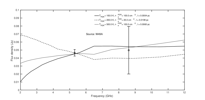
Figure 5: PDR model results for W49. See Figure 4 for details.

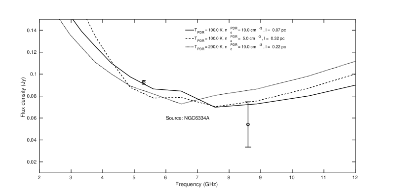
Figure 6: PDR model results for NGC 6334A. See Figure 4 for details.

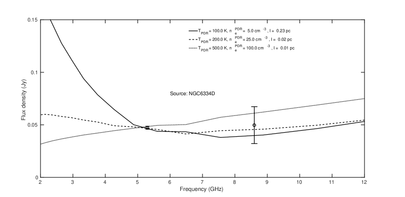
Figure 7: PDR model results for NGC 6334D. See Figure 4 for details.

Table 1: H ii Region Continuum Parameters

				R.A.				Decl.
	R.A. (B1950)	Decl. (B1950)	$R_{\rm Sun}$	$T_{\rm C}$	$\sigma\,T_{\rm C}$	$\Theta$	$\sigma\,\Theta$	$T_{\rm C}$	$\sigma\,T_{\rm C}$	$\Theta$	$\sigma\,\Theta$
Name	(hh:mm:ss.s)	(dd:mm:ss)	(kpc)	(K)	(K)	(arcsec)	(arcsec)	(K)	(K)	(arcsec)	(arcsec)
W3 A	02:21:56.9	$+$61:52:40.0	2.1	70.42	0.35	360.25	2.14	69.34	0.19	154.37	0.62
W49 A	19:07:52.1	$+$09:01:08.0	11.8	58.66	0.57	202.66	2.38	59.53	0.15	161.33	0.53
NGC6334 A	17:16:57.8	$-$35:51:45.0	1.7	34.37	0.11	208.69	1.06	34.48	0.17	182.41	1.84
NGC6334 D	17:17:23.0	$-$35:46:20.0	1.7	39.91	0.16	246.70	1.86	38.20	0.10	189.84	0.81

Table 2: Radio Recombination Line Parameters

		$T_{\rm L}$	$\sigma\,T_{\rm L}$	$\Delta{V}$	$\sigma\,\Delta{V}$	$V_{\rm LSR}$	$\sigma\,V_{\rm LSR}$	$t_{\rm intg}$	rms
Name	Element	(mK)	(mK)	($\,{\rm km\,s^{-1}}$)	($\,{\rm km\,s^{-1}}$)	($\,{\rm km\,s^{-1}}$)	($\,{\rm km\,s^{-1}}$)	(hr)	(mK)
W3	H	3159.30	6.38	29.795	0.040	$-$40.462	0.010	10.7	11.20
$\cdots$	H	416.86	6.41	9.076	0.139	$-$41.069	0.037	$\cdots$	11.20
$\cdots$	He	326.76	1.23	24.848	0.113	$-$40.222	0.046	$\cdots$	8.42
$\cdots$	C	342.99	2.73	5.525	0.077	$-$39.054	0.035	$\cdots$	8.42
$\cdots$	X	80.08	2.45	6.519	0.400	$-$46.556	0.163	$\cdots$	8.42
W49	H	2918.63	2.77	29.159	0.032	8.345	0.014	29.6	12.23
$\cdots$	He	296.59	0.74	24.039	0.084	8.857	0.032	$\cdots$	4.77
$\cdots$	C	93.06	3.29	7.856	0.307	13.580	0.192	$\cdots$	4.77
$\cdots$	C	96.66	1.47	9.608	0.536	4.464	0.203	$\cdots$	4.77
$\cdots$	X	11.35	1.59	5.805	1.43	$-$6.386	0.539	$\cdots$	4.77
NGC6334 A	H	2130.88	1.54	26.827	0.023	1.035	0.009	21.4	6.75
$\cdots$	He	125.76	0.54	23.834	0.118	2.671	0.050	$\cdots$	4.44
$\cdots$	C	184.97	1.17	5.212	0.042	$-$2.478	0.017	$\cdots$	4.44
$\cdots$	X	39.97	1.20	5.083	0.204	$-$11.141	0.077	$\cdots$	4.44
NGC6334 D	H	3083.08	1.63	22.270	0.014	$-$3.375	0.006	23.7	7.59
$\cdots$	He	280.85	0.84	15.999	0.062	$-$3.713	0.024	$\cdots$	4.73
$\cdots$	C	94.54	0.96	7.022	0.112	$-$2.722	0.040	$\cdots$	4.86
$\cdots$	X	20.03	1.08	5.492	0.509	$-$11.888	0.172	$\cdots$	4.86

Note. — Spectral line parameters correspond to the average of 7 RRLs ($104\alpha-110\alpha$).

Table 3: Spherical Homogeneous H ii Region Models

	$T_{\rm e}$	$\theta_{\rm sph}$	$n_{\rm e}$	Peak $EM$	Log10($N_{\rm L}$)	Spectral
Name	($K$)	(arcmin)	(cm-3)	$10^{5}\,$(pc cm-6)	(photons s-1)	Type
W3 A	8000	5.24	522	7.23	49.63	O4.5
W49 A	8500	3.26	318	6.22	50.82	$<$O3
NGC 6334 A	8000	3.89	526	3.54	48.97	O7.5
NGC 6334 D	7000	4.56	480	3.84	49.13	O7

Table 4: Radio Recombination Line PDR Model Constraints

		$T_{\rm L}$	$\sigma\,T_{\rm L}$	$\Delta{V}$	$\sigma\,\Delta{V}$	$V_{\rm LSR}$	$\sigma\,V_{\rm LSR}$	$S_{\nu}$	$\sigma\,S_{\nu}$
Name	RRL	(mK)	(mK)	($\,{\rm km\,s^{-1}}$)	($\,{\rm km\,s^{-1}}$)	($\,{\rm km\,s^{-1}}$)	($\,{\rm km\,s^{-1}}$)	(mJy)	(mJy)
W3 A	$<$${\rm C}104\alpha$-${\rm C}110\alpha$$>$	342.99	2.73	5.525	0.077	$-$39.054	0.035	171.5	1.4
	${\rm C}91\alpha$	56.39	4.93	7.68	0.79	$-$40.10	0.33	113.4	9.9
W49 A	$<$${\rm C}104\alpha$-${\rm C}110\alpha$$>$	93.06	3.29	7.856	0.307	13.58	0.192	46.5	1.6
	$<$${\rm C}104\alpha$-${\rm C}110\alpha$$>$	96.66	1.47	9.608	0.536	4.464	0.203	48.3	0.7
	$<$${\rm C}91\alpha$-${\rm C}92\alpha$$>$	24.77	1.79	15.72	1.36	7.33	0.67	49.8	3.6
NGC 6334 A	$<$${\rm C}104\alpha$-${\rm C}110\alpha$$>$	184.97	1.17	5.221	0.042	$-$2.478	0.017	92.5	0.6
	${\rm C}91\alpha$	26.93	3.42	8.34	1.23	$-$3.14	0.52	54.1	6.9
NGC 6334 D	$<$${\rm C}104\alpha$-${\rm C}110\alpha$$>$	94.54	0.96	7.022	0.112	$-$2.722	0.040	47.3	0.5
	${\rm C}91\alpha$	24.73	2.91	9.99	1.37	$-$4.37	0.58	49.7	5.8

Table 5: PDR Model Physical Properties

	$T_{\rm PDR}$	$n_{\rm e}^{\rm PDR}$	$\ell$	$B$
Name	(K)	($\,{\rm cm^{-3}}$)	(pc)	($\mu$G)
W3 A	100	$5-25$	$0.4-0.013$	$140-320$
	200	$5-25$	$1.7-0.048$	$140-320$
W49 A	100	$50-100$	$0.0015-0.0004$	$650-910$
	200	$25-200$	$0.0199-0.0004$	$460-1300$
	500	$5-200$	$3.1-0.0016$	$200-1300$
NGC 6334 A	100	10	0.07	190
NGC 6334 D	100	$5-100$	$0.23-0.0005$	$180-820$
	200	$5-200$	$0.73-0.0004$	$180-1200$
	500	$5-200$	$3.4-0.0017$	$180-1100$

References

- Abel et al. (2005) Abel, N. P., Ferland, G. J., Shaw, G., & van Hoof, P. A. M. 2005, ApJS, 161, 65
- Altenhoff (1960) Altenhoff, W. J. 1960, Veröff Sternwarte Bonn, Nr. 59
- Anderson et al. (2014) Anderson, L. D., Bania, T. M., Balser, D. S., et al. 2014, ApJS, 212, 1
- Arons & Max (1975) Arons, J., & Max, C. E. 1975, ApJ, 196, L77
- Balser (2006) Balser, D. S. 2006, AJ, 132, 2326
- Balser et al. (1995) Balser, D. S., Bania, T. M., Rood, R. T., & Wilson, T. L. 1995, ApJS, 100, 371
- Balser et al. (1999) Balser, D. S., Bania, T. M., Rood, R. T., & Wilson, T. L. 1999, ApJ, 510, 759
- Bania et al. (1997) Bania, T. M., Balser, D. S., Rood, R. T., Wilson, T. L., & Wilson, T. J. 1997, ApJS, 113, 353
- Beckman & Relao (2004) Beckman, J. E., & Relao, M. 2004, Ap&SS, 292, 111
- Brocklehurst & Salem (1977) Brocklehurst, M., & Salem, M. 1977, CoPhC, 13, 39
- Brogan & Troland (2001) Brogan, C. L., & Troland, T. H. 2001, ApJ, 560, 821
- Crutcher (1999) Crutcher, R. M. 1999, ApJ, 520, 706.
- Crutcher (2012) Crutcher, R. M. 2012, ARA&A, 50, 29.
- De Pree et al. (1997) De Pree, C. G., Mehringer, D. M., & Goss, W. M. 1997, ApJ, 482, 307
- Ferland (2001) Ferland, G. 2001, PASP, 113, 41
- Gordon & Sorochenko (2009) Gordon, M. A., & Sorochenko, R. L. 2009, Radio Recombination Lines. Their Physics and Astronomical Applications (ASSL, Vol. 282; New York: Springer)
- Kraemer et al. (2000) Kraemer, K., E., Jackson, J. M., Lane, A. P., & Paglione, T. A. D. 2000, ApJ, 542, 946
- MacLow & Klessen (2004) MacLow M.-M., & Klessen R.S. 2004., RvMP 76, 125
- Marscher, et al. (1993) Marscher, A. P., Moore, E. M., & Bania, T. M. 1993, ApJ, 419, L101
- McKee & Ostriker (2007) McKee C. F., Ostriker E. C. 2007, ARA&A, 45, 565
- McKee & Zweibel (1995) McKee, C. F., & Zweibel, E. G. 1995, ApJ, 440, 686
- Minter & Spangler (1996) Minter, A. H., & Spangler, S. R. 1996, ApJ, 458, 194
- Morris et al. (1974) Morris, M., Zuckerman, B., Turner, B. E., & Palmer, P. 1974, ApJ, 192, L27
- Morton (1974) Morton, D. C. 1974, ApJ, 193, L35
- Mouschovias (1975) Mouschovias, T. Ch. 1975, Ph.D. thesis, Univ. California, Berkeley
- Nakamura & Li (2005) Nakamura F., & Li Z.-Y. 2005, ApJ, 631, 411
- Natta et al. (1994) Natta, A., Walmsley, C. M., & Tielens, A. G. G. M. 1994, ApJ, 428, 209
- Neckel (1978) Neckel, T. 1978, A&A, 69, 51
- Parker (1979) Parker, E. N. 1979, Cosmical Magnetic Fields (International Series of Monographs on Physics; New York: Oxford Univ. Press)
- Quireza et al. (2006) Quireza, C., Rood, R. T., Balser, D. S., & Bania, T. M. 2006, ApJS, 165, 338
- Roberts et al. (1993) Roberts, D. A., Crutcher, R. M., Troland, T. H., & Goss,W. M. 1993, ApJ, 412, 675
- Roshi (2007) Roshi, D. A. 2007, ApJ, 658, L41
- Roshi et al. (2005) Roshi, D. A., Balser, D. S., Bania, T. M., Goss, W. M., & De Pree, C. G. 2005, ApJ, 625, 181
- Roshi et al. (2006) Roshi, D. A., De Pree, C. G., Goss, W. M., & Anantharamaiah, K. R. 2006, ApJ, 644, 279
- Roshi et al. (2014) Roshi, D. A., Goss, W. M., Jeyakumar, S. 2014, ApJ, 793, 83
- Sarma et al. (2000) Sarma, A. P., Troland, T. H., Roberts, D. A., & Crutcher, R. M. 2000, ApJ, 533, 271
- Shaver (1975) Shaver, P. A. 1975, Parmana, 5, 1
- Shu et al. (1987) Shu F. H., Adams F. C., Lizano S. 1987, ARA&A, 25, 23
- Tieftrunk et al. (1997) Tieftrunk, A. R., Gaume, R. A., Claussen, M. J.,Wilson, T. L., & Johnston, K. J. 1997, A&A, 318, 931
- Vacca et al. (1996) Vacca, W. D., Garmany, C. D., & Shull, J. M. 1996, ApJ, 460, 914
- Walmsley & Watson (1982) Walmsley, C. M., & Watson, W. D. 1982, ApJ, 260, 317
- Wenger et al. (2013) Wenger, T. V., Bania, T. M., Dana, S., & Anderson, L. D. 2013, ApJ, 764, 34
- Wood & Churchwell (1989) Wood, D. O. S., & Churchwell, E. 1989, ApJS, 69, 831
- Zuckerman & Palmer (1968) Zuckerman, B., & Palmer, P. 1968, ApJ, 153, L145