The size of the pion from full lattice QCD with physical $u$, $d$, $s$ and $c$ quarks

Abstract

We present the first calculation of the electromagnetic form factor of the $\pi$ meson at physical light quark masses. We use configurations generated by the MILC collaboration including the effect of $u$, $d$, $s$ and $c$ sea quarks with the Highly Improved Staggered Quark formalism. We work at three values of the lattice spacing on large volumes and with $u$/$d$ quark masses going down to the physical value. We study scalar and vector form factors for a range in space-like $q^{2}$ from 0.0 to -0.1 $\mathrm{GeV}^{2}$ and from their shape we extract mean square radii. Our vector form factor agrees well with experiment and we find $\langle r^{2}\rangle_{V}=0.403(18)(6)\,\mathrm{fm}^{2}$. For the scalar form factor we include quark-line disconnected contributions which have a significant impact on the radius. We give the first results for SU(3) flavour-singlet and octet scalar mean square radii, obtaining: $\langle r^{2}\rangle_{S}^{\mathrm{singlet}}=0.506(38)(53)\mathrm{fm}^{2}$ and $\langle r^{2}\rangle_{S}^{\mathrm{octet}}=0.431(38)(46)\mathrm{fm}^{2}$. We discuss the comparison with expectations from chiral perturbation theory.

I Introduction

The electromagnetic form factor of the charged $\pi$ meson parameterises the deviations from the behaviour of a point-like particle when struck by a photon. These deviations result from the internal structure of the $\pi$ i.e. its quark constituents and their strong interaction. The form factor is calculable in QCD but a fully nonperturbative treatment is necessary at the small (negative) values of 4-momentum transfer, $q^{2}$, covered by direct model-independent experimental determination of the vector form factor Amendolia et al. (1986) from $\pi-e$ scattering. The experimental error is 1-1.5% in the region up to $|q^{2}|=0.1\mathrm{GeV}^{2}$ and so a lattice QCD calculation of the form factor there can provide a stringent test of QCD. This is complementary to tests of QCD through calculation of meson masses and of decay constants that parameterise meson annihilation, for example to a $W$ boson Davies et al. (2004); Dowdall et al. (2013).

In the nonrelativistic limit, where $q^{2}\approx-(\vec{q})^{2}$, the vector form factor, $f_{+}(q^{2})$, can be viewed as the Fourier transform of the electric charge distribution. The mean squared radius obtained by integrating over this distribution is then given by

$$\langle r^{2}\rangle=6\frac{df_{+}(q^{2})}{dq^{2}}\bigg{|}_{q^{2}=0}.$$ (1)

This is adopted more generally as a definition of $\langle r^{2}\rangle$, since it is useful to have a single number with which to characterise the shape of the form factor. We will use it here to compare the ‘size’ of the $\pi$ derived from our form factor with that obtained from experiment.

The calculation of $\langle r^{2}\rangle$ from lattice QCD is complicated by the fact that the result is very sensitive to the mass of the $\pi$. The mean square radius diverges as $m_{\pi}^{2}\rightarrow 0$ when the $\pi$ meson cloud surrounding the $\pi$ becomes of infinite range Gasser and Leutwyler (1984). It has been numerically too expensive until recently to include $u/d$ quarks with their physically very light masses in lattice QCD calculations. Results have instead had to be extrapolated to the physical point from heavier masses using chiral perturbation theory. The lightest $\pi$ meson mass used in earlier calculations of the electromagnetic form factor has been in the range of 250-400 MeV, i.e. approximately twice the physical value or more. Results range from multiple values of the lattice spacing including the effect of $u$ and $d$ sea quarks Brommel et al. (2007); Frezzotti et al. (2009); Brandt et al. (2013) to those with only a single lattice spacing including the effect of $u$, $d$ sea quarks Aoki et al. (2009) or, more realistically, $u$, $d$ and $s$ sea quarks Aoki et al. (2015); Nguyen et al. (2011); Boyle et al. (2008). See also Fukaya et al. (2014) for a calculation in the $\varepsilon$ regime. A mean square radius can similarly be defined for the scalar form factor. Earlier results, again for relatively heavy values of the $\pi$ meson mass, have been obtained with $u$ and $d$ sea quarks (only) in Aoki et al. (2009); Guelpers et al. (2014); Gülpers et al. (2015).

Here we give results for both vector and scalar form factors for $\pi$ mesons made of physical $u/d$ quarks and including a fully realistic quark content in the sea, with physical $u$, $d$, $s$ and $c$ quarks. We also work with three different values of the lattice spacing. This enables good control of systematic errors both from $m_{\pi}$ and from discretisation. Our lattices have large volumes with a minimum spatial size of 4.8 fm.

The vector form factor is accessible in experiment and, as we shall see, our results can be directly compared to the experimental data with no extrapolation.

The scalar form factor cannot be obtained directly by experiment but information on it can be extracted by applying chiral perturbation theory to the $\pi$ decay constant and to $\pi-\pi$ scattering Gasser and Leutwyler (1984, 1983); Colangelo et al. (2001). An additional ingredient in the lattice QCD calculation in this case is the need to include quark-line disconnected contributions. The expectation from chiral perturbation theory Jüttner (2012) is for the disconnected contribution to the form factor at $q^{2}=0$ to be small but for the impact on the radius as defined in eq. (1) to be substantial. Our results are very much in line with expectations from chiral perturbation theory and we are able to distinguish disconnected contributions coming from $u/d$ and $s$ quark loops.

Section II describes how the lattice calculation is done and gives details of the results. Our results are compared to experiment, to chiral perturbation theory expectations, and to other lattice calculations in Section III and Section IV gives our conclusions, looking forward to improved calculations in future.

II Lattice Calculation

For the lattice QCD calculation we use the Highly Improved Staggered Quark (HISQ) action Follana et al. (2007), which has been demonstrated to have very small discretisation errors Donald et al. (2012); Dowdall et al. (2013). We use gluon field configurations generated by the MILC collaboration Bazavov et al. (2010, 2013) that include $u$, $d$, $s$ and $c$ sea quarks using the HISQ action along with a fully $\mathcal{O}(\alpha_{s}a^{2})$ improved gluon action Hart et al. (2009). The ensembles that we use here have light quark masses $m_{u}=m_{d}=m_{l}$ with $m_{l}$ and hence $m_{\pi}$ close to its physical value. The parameters of the ensembles are given in Table 1.

Table 1: The MILC gluon field ensembles (sets) used here Bazavov et al. (2010, 2013). The lattice spacing, $a$, is determined using the $w_{0}$ parameter Borsanyi et al. (2012), and has a correlated 0.5% uncertainty from the physical value of $w_{0}$, fixed using $f_{\pi}$ Dowdall et al. (2013). Set 1 will be referred to “very coarse”, 2 as “coarse” and 3 as “fine”. Columns 3, 4 and 5 give the sea quark masses in lattice units ($m_{u}=m_{d}=m_{l}$). $L_{s}$ and $L_{t}$ are the lengths in lattice units in space and time directions for each lattice. The number of configurations that we have used in each set is given in the seventh column. The final column gives the values of the end-point of the 3-point function, $T$, in lattice units.

Set	$a$/fm	$am_{l,sea}$	$am_{s,sea}$	$am_{c,sea}$	$L_{s}\times L_{t}$	$n_{\mathrm{cfg}}$	$T$
1	0.1509	0.00235	0.0647	0.831	32$\times$48	1000	9,12,15
2	0.1212	0.00184	0.0507	0.628	48$\times$64	1000	12,15,18
3	0.0879	0.0012	0.0363	0.432	64$\times$96	223	16,21,26

On these configurations we generate HISQ light quark propagators with the same mass as that of the sea light quarks. We use a local random wall source Dowdall et al. (2013) and 4 time sources per configuration for high statistics. The propagators are combined into $\pi$ meson correlation functions (2-point correlators) that create a $\pi$ meson at time 0 and destroy it at time $t^{\prime}$ and correlation functions that allow for interaction with a current $J$ at an intermediate time, $t$, between a $\pi$ meson source at 0 and sink at $T$ (3-point correlators). These are illustrated in Fig. 1. Results at all $t^{\prime}(t)$ values are obtained for 2(3)-point functions and we also use three values for $T$ in the 3-point functions, so that our fits can map out fully the $t$ and $T$ dependence for improved accuracy. When $J$ is a vector current we need to consider only one 3-point diagram for the flavour non-singlet $\pi$. This is shown as the central diagram of Fig. 1 in which the current $J$ is inserted into one of the legs of the 2-point function. We simply multiply by 2 to allow for its insertion into the other leg. The ‘disconnected diagram’ which is the product of a $\pi$ 2-point function and a closed quark loop coupled to $J$ is shown as the lower diagram of Fig. 1. This vanishes for vector $J$ in the ensemble average because it is odd under charge-conjugation Draper et al. (1989). For scalar $J$ this diagram needs to be included and different combinations of flavours of quarks in the closed quark loop give rise to different form factors.

The $\pi$ mesons in our correlators are the Goldstone mesons whose mass vanishes with $m_{l}$. We ensure this by using the local $\gamma_{5}$ operator at source and sink. In staggered quark parlance this is the $\gamma_{5}\otimes\gamma_{5}$ operator. For $J$ we use a symmetric 1-link point-split spatial vector current, $V_{i}$, or a local scalar current, $S$. A gluon field is included in the vector current to make it gauge-covariant. Both of these are ‘tasteless’ staggered quark operators ($\gamma_{i}\otimes 1$ and $1\otimes 1$) and so can be used in a 3-point function with the Goldstone meson at source and sink.

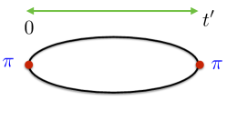
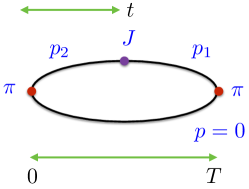
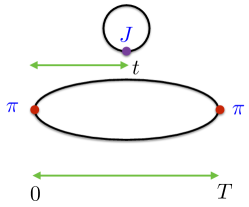
Figure 1: 2-point (top) and 3-point quark-line-connected (middle) and quark-line disconnected (bottom) correlators.

We work with several $\pi$ meson spatial momenta by generating light quark propagators with a phase included on the spatial gluon links. This is equivalent to introducing a phase into the boundary condition on the field Guadagnoli et al. (2006), which gives a momentum to the quark. This is referred to as using ‘twisted boundary conditions’. As illustrated in the central diagram of Fig. 1 we choose the spectator quark in the 3-point function to have zero momentum and give momenta $p_{1}$ and $p_{2}$ to the quarks that interact with the current. Both momenta are chosen to be in the $(1,1,1)$ direction. By using various values of $p_{1}$ and $p_{2}$ we can obtain 3-point functions at several different small values of squared 4-momentum transfer, $q^{2}$.

II.1 Vector Form Factor

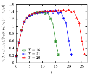
Figure 2: Results for the ratio of the 3-point correlator containing a vector current to the product of appropriate 2-point correlators for the pion on fine ensemble set 3. The ratio for the 3 different values of $T$ are plotted as a function of $t$ with a $\pi$ of momentum zero on the left, and momentum $ap=0.0363$ on the right. Note that this figure is to illustrate the quality of our results; we do not use this ratio to extract ground-state parameters. Instead we perform a simultaneous fit to multiple exponentials for both the 2-point and 3-point correlators as described in the text.

For the vector current case we have a set of 2-point and 3-point quark-line connected correlators at various values of $p_{1}$ and $p_{2}$ on each ensemble. The quality of our results is illustrated for one ensemble and set of momenta in Figure 2. The 2-point and 3-point correlators are all fit simultaneously using Bayesian methods Lepage et al. (2002) that allow us to include the effect of excited states, both ‘radial’ excitations and, because we are using staggered quarks, opposite parity mesons that give oscillating terms. Since the oscillating terms are absent for zero-momentum $\pi$ mesons they are small here, but we nevertheless include them in our fits. Having 3-point correlators from multiple $T$ values is also important in taking account of excited states. Fitting multiple momenta simultaneously allows us to take account of correlations between the correlators.

The fit form for the 2-point function with source at 0 and sink at $t^{\prime}$ and spatial momentum, $p$, is:

$$C_{2pt}(p,0,t^{\prime}) = \sum_{i}b_{i}^{2}(p)\mathrm{fn}(E_{i}(p),t^{\prime})+\mathrm{o.p.t.}$$

$$\mathrm{fn}(E,t) = e^{-Et}+e^{-E(L_{t}-t)}.$$ (2)

Opposite parity terms (o.p.t.) are similar to the terms given explicitly above but with factors of $(-1)^{t^{\prime}/a}$. For the 3-point function Koponen et al. (2013); Donald et al. (2014):

$$C_{3pt}(p_{1},p_{2},0,t,T)=\sum_{i,j}\big{[}b_{i}(p_{1})\mathrm{fn}(E_{i}(p_{1}),t)\times\\ J_{i,j}(p_{1},p_{2})b_{j}(p_{2})\mathrm{fn}(E_{j}(p_{2}),T-t)\big{]}+\mathrm{o.p.t.}$$ (3)

Prior values and widths are taken as: ground-state energy, 10% width; splitting between ground-state and excited energies, 650 MeV with 50% width; splitting between ground-state and lowest oscillating state, 500 MeV with 50% width; amplitudes, 0.01(1.0) for normal states and 0.01(0.5) for oscillating states; matrix elements, 0.01(1.0) for vector currents. We take the result from a 6 exponential fit (with 6 oscillating exponentials) to obtain the vector form factor.

Table 2: Upper table: Results for $\pi$ energies in lattice units at the different spatial momenta used on each set, as well as the corresponding amplitudes from the 2-point functions. The values given here come from the simultaneous fit of 2-point correlators with 3-point correlators containing a vector current. Results for 2-point parameters from the fit of 2-point correlators with 3-point correlators including a scalar current are in agreement. $\pi$ results at zero momentum agree with those in Dowdall et al. (2013); McNeile et al. (2013), but are not the same because the fits used here also include 3-point functions.
Lower table: Results for unrenormalised form factors at $q^{2}$ values corresponding to different combinations of $\pi$ momenta (from the upper table) at source and sink. The results at $q^{2}=0$ come from using the lowest non-zero spatial momentum for both $p_{1}$ and $p_{2}$. The scalar form factor results given are for the connected 3-point function only.

Set	$pa$	$aE_{\pi}$	$a^{3/2}b$	$pa$	$aE_{\pi}$	$a^{3/2}b$	$pa$	$aE_{\pi}$	$a^{3/2}b$
1	0.0	0.10167(5)	0.4845(3)	0.0623	0.11921(6)	0.4465(2)	0.2490	0.2669(9)	0.2936(14)
2	0.0	0.08159(3)	0.35773(15)	0.05	0.09569(4)	0.32981(14)	0.16482	0.1840(2)	0.2375(3)
	0.2	0.2161(4)	0.2193(5)
3	0.0	0.05720(3)	0.23272(15)	0.0363	0.06767(4)	0.21397(13)	0.1451	0.1546(5)	0.1400(5)
Set	$q^{2}a^{2}$	$f_{+}(q^{2})/Z_{V}$	$f_{0}^{\mathrm{conn}}(q^{2})/Z_{S}$	$q^{2}a^{2}$	$f_{+}(q^{2})/Z_{V}$	$f_{0}^{\mathrm{conn}}(q^{2})/Z_{S}$	$q^{2}a^{2}$	$f_{+}(q^{2})/Z_{V}$	$f_{0}^{\mathrm{conn}}(q^{2})/Z_{S}$
1	0.0	0.837(3)	2.163(6)	-0.0036	0.832(4)	2.143(4)	-0.0346	0.761(8)	1.98(2)
	-0.0751	0.678(10)	1.82(2)
2	0.0	0.852(2)	1.769(3)	-0.0023	0.847(3)	1.753(2)	-0.0054	0.838(4)	1.719(6)
	-0.0167	0.797(3)	1.656(5)	-0.0220	0.782(4)	1.623(7)	-0.0384	0.731(5)	1.542(7)
	-0.0480	0.702(8)	1.500(8)
3	0.0	0.841(2)	1.330(4)	-0.0012	0.842(4)	1.321(3)	-0.0116	0.775(7)	1.210(10)
	-0.0254	0.692(8)	1.125(10)

The ground-state parameters are given by $i=j=0$ in eqs. (2) and (3) and are our key results. By matching to a continuum correlator with a relativistic normalisation of states and allowing for a renormalisation of the lattice current, we see that the matrix elements between the ground state mesons that we want to determine are given by:

$$\langle\pi(p_{1})|J|\pi(p_{2})\rangle=Z\sqrt{4E_{0}(p_{1})E_{0}(p_{2})}J_{0,0}(p_{1},p_{2}).$$ (4)

The matrix element is related to the form factor for the vector current via:

$$\langle\pi(p_{1})|V_{i}|\pi(p_{2})\rangle=f_{+}(q^{2})(p_{1}+p_{2})_{i}$$ (5)

The vector matrix element can be normalised using the fact that $f_{+}(0)=1$ for a conserved current (inserted in either the quark or the antiquark legs in Fig. 1), and we can therefore determine $Z$ by demanding that condition for our current. $f_{+}(0)$ is determined at $q^{2}=0$ for spatial $V_{i}$ by setting $p_{1}=p_{2}\neq 0$.

II.1.1 Results

Table 2 gives results for the $\pi$ energies and 2-point amplitudes as a function of momentum. A good test of discretisation errors is to determine the speed of light, $c^{2}$ from $(E^{2}-m^{2})/p^{2}$. From Table 2 we see that $c^{2}$ deviates from 1 at most by 2(1)% at the largest momenta. Another test is to compare the scaling of amplitudes to the expected $1/\sqrt{E}$ behaviour for a pseudoscalar. Again we see good agreement, with deviations at most 3(1.5)%.

Table 2 also gives the raw (unrenormalised) form factors for various $q^{2}$ values obtained from different combinations of momenta (in positive and negative) directions at source and sink. The statistical errors on the form factors are 0.5-3%. By dividing the values at non-zero $q^{2}$ by the value at $q^{2}=0$ we obtain normalised values for $f_{+}$. $f_{+}$ is plotted against $q^{2}$ in Fig. 3 for all three sets along with the results from experiment Amendolia et al. (1986). The agreement with experiment is good, reflecting the fact that our results correspond to physical $\pi$ masses.

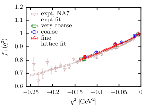
Figure 3: Lattice QCD results for the vector form factor on each ensemble compared directly to the experimental results from Amendolia et al. (1986). Fit curves for both experiment and lattice QCD results are given to a ‘monopole’ form.

In fitting a functional form in $q^{2}$ to our results to extract a mean squared radius, we use the same form as that used for the experimental results Amendolia et al. (1986), but including allowance for finite lattice spacing effects. We also fit over a similar range of $q^{2}$ values. We use:

$$f(q^{2})=\frac{1}{1+c_{a^{2}}(\Lambda a)^{2}+c_{a^{4}}(\Lambda a)^{4}-\langle r^{2}\rangle q^{2}/6}$$ (6)

(note that $q^{2}$ is negative), where

$$\langle r^{2}\rangle_{V}(a,\delta m_{\mathrm{sea}},m_{\pi})=$$

$$\langle r^{2}\rangle_{V}\bigg{[}1+b_{a^{2}}(\Lambda a)^{2}+b_{a^{4}}(\Lambda a)^{4}+\frac{b_{\mathrm{sea}}\delta m_{\mathrm{sea}}}{10m_{s,\mathrm{phys}}}\bigg{]}$$

$$- \frac{1}{\Lambda_{\chi}^{2}}\ln\bigg{(}\frac{m^{2}_{\pi}}{m^{2}_{\pi,\mathrm{phys}}}\bigg{)}.$$

Here $c_{a^{n}}$ and $b_{a^{n}}$ allow for discretisation effects in the normalisation of $f_{+}$ and in $\langle r^{2}\rangle$ respectively. We take $\Lambda$ = 500 MeV and allow priors on the $b$ and $c$ fit parameters of 0.0(1.0) for $b_{a^{4}}$ and $c_{a^{4}}$ and 0.0(0.3) on $b_{a^{2}}$ and $c_{a^{2}}$ (since tree-level $a^{2}$ errors are absent in this calculation). We allow a prior width on the physical result for the mean squared radius, $\langle r^{2}\rangle_{V}$ of 25%. The term with coefficient $b_{\mathrm{sea}}$ allows for mistuning of sea quark masses. From chiral perturbation theory a term linear in the quark masses is expected, and it is convenient to take this term as a ratio to another quark mass so that factors of the quark mass renormalisation cancel. The factor of 10 multiplying $m_{s,\mathrm{phys}}$ gives a value close to the chiral scale, $\Lambda_{\chi}$. The mistuning of the sea masses is defined as $\sum_{u,d,s}(m_{q}-m_{q}^{\mathrm{tuned}})$ and values of $\delta m_{\mathrm{sea}}/m_{s,\mathrm{phys}}$ values for these ensembles are tabulated in Chakraborty et al. (2015). The values are all less than 0.05, but not zero because of mistuning of the sea $s$ quark mass.

The final logarithmic term in eq. (II.1.1) comes from chiral perturbation theory Gasser and Leutwyler (1984) and is the source of the divergence in the radius as $m_{\pi}\rightarrow 0$. We use it, rescaling the argument of the logarithm so that it vanishes at the physical pion mass, to make small adjustments for the fact that our $u/d$ quark masses are not exactly at their physical values (in fact they are slightly too low). $\Lambda_{\chi}$ = 1.16 GeV. Because we are very close to the physical light quark mass point we do not need to include further terms in a chiral perturbation theory expansion since they will be negligible.

We apply the functional form of eq. (6) and (II.1.1) to our result taking account of the correlations between results at different values of $q^{2}$ obtained on a given ensemble. The fit has $\chi^{2}/\mathrm{dof}=0.9$ and gives the physical result for the electric charge radius of the $\pi$ of $\langle r^{2}\rangle_{V}=$ 10.35(46) ${\mathrm{GeV}}^{-2}$, or 0.403(18) $\mathrm{fm}^{2}$.

We can also use the final logarithmic term in eq. (II.1.1) to estimate the impact of isospin and electromagnetic effects by varying the value of $m_{\pi,\mathrm{phys}}$ used there. The physical value of $m_{\pi}$ corresponding to our lattice world in which $u$ and $d$ quark masses are equal and there is no electromagnetism is $m_{\pi^{0}}$ = 0.135 GeV Aubin et al. (2004), and we use this for our central value above. The experimental results correspond to $m_{\pi^{+}}$ = 0.139 GeV and we substitute that for the physical value in the logarithm to assess the uncertainty from the fact that the real world has different $u/d$ quark masses and the quarks have electric charge. This gives an estimate for the systematic uncertainty from isospin/electromagnetism of 0.5%.

We must also include a systematic uncertainty from working on lattices with finite spatial volume, albeit large. Finite volume effects are small on these lattices for the $\pi$ mass and decay constant Dowdall et al. (2013) and effects of similar size are expected in the form factor at fixed $q^{2}$. Because the mean squared radius is defined from the small difference in values for the form factor as $q^{2}$ moves away from zero (where the form factor is defined to be 1), a small effect on the form factor at non-zero $q^{2}$ can become a significant effect on the radius. These effects can be estimated from chiral perturbation theory. Continuum chiral perturbation theory is a good guide here and we do not need staggered chiral perturbation theory because, as shown in Colquhoun et al. (2015), staggered quark taste-effects which might be expected to affect $\pi$ masses appearing in chiral loops in fact tend to cancel against associated hairpin diagrams. It turns out that this cancellation happens for a wide range of quantities (including decay constants and form factors) for a specific value of the hairpin coefficients that seems to be close to the value obtained in practice. We therefore use continuum analyses and specifically results from analyses that are relevant to our use of twisted boundary conditions Jiang and Tiburzi (2007); Bijnens and Relefors (2014) because this modifies the expected finite-volume dependence. From Jiang and Tiburzi (2007) the relative finite volume effect in the vector squared-radius varies in the range 1–1.5% for lattice sizes that we use in the range 4.8 fm to 5.8 fm for physical $\pi$ masses. Note that the direction of the finite-volume effect is such that the radius would be larger in the infinite volume limit. We do not make a correction for this but include an uncertainty of 1.5% for finite volume effects.

Table 3: Error budget for the mean square radii of the $\pi$, as a percentage of the final answer. See the discussion in the text for a description of each component.

	$\langle r^{2}\rangle_{V}$	$\langle r^{2}\rangle_{S}^{\mathrm{conn}}$	$\langle r^{2}\rangle_{S}^{\mathrm{singlet/octet}}$
statistics/fitting	4.5	5	7.5/8.5
isospin/electromagnetism	0.5	3	3
finite volume	1.5	10	10
total	4.8	12	13/14

Our error budget for $\langle r^{2}\rangle_{V}$ is given in Table 3. Adding the systematic uncertainties in quadrature as the second uncertainty gives our result:

$$\langle r^{2}\rangle_{V}^{(\pi)}=0.403(18)(6)\,{\mathrm{fm}}^{2}$$ (8)

to be compared to 0.431(10) $\mathrm{fm}^{2}$ from the experimental results of Amendolia et al. (1986) using the same fit form. The Particle Data Group Olive et al. (2014) give a mean square radius from averaging over several experimental results of 0.452(11) $\mathrm{fm}^{2}$.

II.2 Scalar Form Factor

II.2.1 Results for the connected contribution

We begin by discussing our results for the connected contribution to the scalar form factor of the $\pi$. This is the result calculated from 3-point functions of the form sketched in the central diagram of Fig. 1 in which the scalar current is composed of the light quarks which are the valence quarks of the $\pi$. Although this form factor does not correspond to a physically realisable process (even if we had a particle with which to produce a scalar current) it is nevertheless possible and useful to compare different lattice QCD calculations for it. Different formalisms within lattice QCD should give the same results in the continuum and chiral limits for the mean square radius from the connected scalar form factor. A key issue, to be discussed further below, is then how big the additional contribution is from quark-line disconnected diagrams.

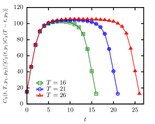
Figure 4: Results for the ratio of the 3-point connected correlator containing a scalar current to the product of appropriate 2-point correlators for the pion on fine ensemble set 3. The ratio for the 3 different values of $T$ are plotted as a function of $t$ with a $\pi$ of momentum zero on the left, and momentum $ap=0.0363$ on the right. Note that this figure is to illustrate the quality of our results; we do not use this ratio to extract ground-state parameters. Instead we perform a simultaneous fit to multiple exponentials for both the 2-point and 3-point correlators as described in the text.

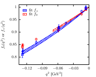
Figure 5: Comparison of our lattice QCD results for the pion vector form factor (blue) with the connected part of the pion scalar form factor (red). Results from set 1 are shown as open squares, set 2 as circles and set 3 as triangles. The hashed curves give the fit to the form factors described in the text (using a smaller $q^{2}$ range in the scalar case than the vector).

The calculation for the connected scalar form factor proceeds in an identical way to that of the vector form factor discussed in Section II.1. We calculate the 3-point function given as the central figure of Fig. 1 with a scalar current made from light quarks inserted as $J$. We use the same light quark propagators and 2-point functions as for the vector case. The quality of our results is illustrated for one ensemble and set of momenta in Fig. 4 (we use the same ensemble and set of momenta as in Fig. 2).

We fit the 2-point and 3-point correlators simultaneously (but in a separate fit from the vector case) as a function of $t$, $t^{\prime}$ and $T$ as given in eqs. (2) and (3). The priors are taken to be the same as in the vector case except that the prior width on the scalar matrix element is taken to be much larger, reflecting expectations on its value given below. We take the prior width on the scalar matrix element to be 20.0 on the very coarse ensemble and 25.0 on the coarse and fine ensembles.

The ground-state matrix element for the scalar current is related to the parameter $J_{0,0}$ extracted from our fits as in eq. (4). In turn the matrix element is related to the form factor that we wish to extract by

$$\langle\pi(p_{1})|S|\pi(p_{2})\rangle^{\mathrm{conn}}=Af_{0}^{\mathrm{conn}}(q^{2})$$ (9)

where $A$ is a normalisation factor. Our scalar current made from HISQ quarks is absolutely normalised Na et al. (2010). If we had included disconnected diagrams associated with the scalar current we would be able to write, from the Feynman-Hellmann theorem,

$$\langle\pi(p_{1})|S|\pi(p_{2})\rangle=f_{0}(q^{2})\frac{\partial m_{\pi}^{2}}{2\partial m_{l}},$$ (10)

with $f_{0}(0)=1$, $A=(\partial m_{\pi}^{2}/\partial m_{l})/2$ and we take the same $m_{l}$ value for valence and sea $l$ quarks. The factor of 2 on the right-hand side comes from the fact that we are inserting a scalar current in only one propagator to make the 3-point correlator and the $\pi$ has two valence light quarks. For the connected correlator we expect instead that factor $A$ in eq. (9) should be equal to half the derivative of the squared $\pi$ mass with respect to its valence quark mass. This can be tested approximately using $\pi$ and $K$ masses on these ensembles in Dowdall et al. (2013). Comparing $a(m_{K}^{2}-m_{\pi}^{2})/(m_{s}-m_{l})$ (i.e. an approx derivative for a pseudoscalar meson mass) to the result for the unrenormalised $f_{0}^{\mathrm{conn}}(0)/Z_{S}$ (=$A$) from Table 2 shows agreement within 10%, confirming that $A$ does have the expected value. Since here we are chiefly concerned with the shape of the form factor, we simply treat the scalar current as requiring a $Z$ factor, $Z_{S}$, and determine this from the requirement that also $f_{0}(0)=1$.

To determine the mean squared radius associated with the connected scalar form factor we take the same fit as for the vector case, eqs. (6) and (II.1.1), except that the coefficient of the chiral logarithm is now 6. This coefficient applies to the complete scalar form factor but we use it here to estimate conservatively the impact of changing the $\pi$ mass close to the physical point and therefore the uncertainty. We use the same priors on the coefficients as in the vector fit, except that we increase the prior on the physical result for the mean squared radius, since its value is less well-known.

Our fit has a $\chi^{2}/{\mathrm{dof}}$ of 1.1 and gives a physical result, $\langle r^{2}\rangle_{S}^{\mathrm{conn}}$ of 8.97(45) $\mathrm{GeV}^{-2}$ or 0.349(18) $\mathrm{fm}^{2}$. The systematic errors are somewhat larger in the scalar case because of the larger coefficient of the chiral logarithm. Using this we estimate the systematic uncertainty from isospin/electromagnetism at 3%. The larger coefficient for the chiral logarithm also carries with it the implication of larger finite volume effects, potentially by a factor of 6, giving a systematic uncertainty of 10% on our ensembles from this source, allowing for the fact that the mean square radius is slightly smaller than for the vector case.

Adding systematic errors in quadrature our final result for the mean squared radius from the connected scalar form factor is

$$\langle r^{2}\rangle_{S,\mathrm{conn}}^{(\pi)}=0.349(18)(36){\mathrm{fm}}^{2}$$ (11)

Our error budget is given in Table 3. This radius has a central value that is only slightly smaller than the vector form factor radius (eq. (8)). This is illustrated in Fig. 5 in which we compare the lattice results and the fit results for the vector and connected scalar cases.

II.2.2 Results including the disconnected contribution

For the full scalar form factor we need to include the quark-line disconnected contribution from the lower diagram of Fig. 1. We can then define flavour-singlet and flavour-octet scalar currents:

$$S_{\mathrm{singlet}} = 2\overline{l}l+\overline{s}s$$ (12)

$$S_{\mathrm{octet}} = 2\overline{l}l-2\overline{s}s.$$

Scalar form factors for these two currents are then determined by combining the connected scalar form factor of Section II.2.1 with disconnected contributions in appropriate combinations from quark loops made from $l$ quarks or $s$ quarks.

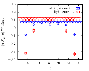
Figure 6: The ratio of 3-point correlator to 2-point correlator for the disconnected contribution for the $\overline{l}l$ (red circles) and $\bar{s}s$ currents (blue squares) to the scalar form factor of the $\pi$ at $q^{2}=0$ on coarse lattices, set 2. The points are the lattice QCD results with statistical errors and the red and blue hashed bands show the ground-state fit result for the $\overline{l}l$ and $\bar{s}s$ contributions, respectively.

For the $q^{2}=0$ case it is particularly simple to calculate the disconnected contributions. Indeed, for the $\overline{s}s$ scalar current this is the $\pi$ meson equivalent of the ‘strangeness in the nucleon’ calculation on which there has been a great deal work in lattice QCD (see, for example, Freeman and Toussaint (2013)). The disconnected contribution for current $\overline{q}q$ is

$$\langle\pi|S_{\overline{q}q}|\pi\rangle^{\mathrm{disc}}=\langle\pi(p)|\overline{q}q|\pi(p)\rangle-\langle\pi(p)|\pi(p)\rangle\langle\overline{q}q\rangle.$$ (13)

The first term is the ensemble average of a $\pi$ meson 2-point function with source at time 0 and sink at time $T$ with a scalar current (condensate) insertion summed over the spatial points making up the timeslice at $t$. The second term in eq. (13) subtracts the product of the vacuum expectation values of the $\pi$ meson correlator and condensate.

With HISQ quarks a convenient way to represent the $\overline{q}q$ condensate is as a sum over a pseudoscalar meson correlator with valence quarks $q$ McNeile et al. (2013). We use an identity Kilcup and Sharpe (1987); McNeile et al. (2013) that relates the quark propagator for staggered quarks on a given gluon field configuration to a product of quark propagators summed over lattice sites:

$$\mathrm{Tr}M^{-1}_{00}=am_{q}\sum_{n}\mathrm{Tr}\left|M^{-1}_{0n}\right|^{2}.$$ (14)

Here $0$ and $n$ are arbitrary lattice sites, $\mathrm{Tr}$ is a color trace and $am_{q}$ is the quark mass in lattice units used in the propagator. The left-hand side of eq. (14) is the negative of the quark loop from site 0 to site 0 needed for the disconnected piece of the scalar current and the the right-hand side is the Goldstone pseudoscalar meson correlator at zero spatial momentum for a quark-antiquark pair of mass $am_{q}$ multiplied by that mass. Since our Goldstone meson correlators here use a random-wall source a sum over a timeslice for lattice site $0$ for the quark loop is done implicitly.

The quantities required to calculate the disconnected contribution for the $s\overline{s}$ current to the scalar form factor at $q^{2}=0$ are then simply $\pi$ meson correlators and those for the pseudoscalar $s\overline{s}$ meson known as the $\eta_{s}$. The $\eta_{s}$ does not correspond to a physical particle but its correlators are nevertheless usefully studied in lattice QCD Davies et al. (2010) and so have been calculated previously Dowdall et al. (2013). To make the 3-point function needed we take a $\pi$ meson correlation function with source at timeslice 0 and sink at time-slice $T$ and a set of $\eta_{s}$ meson correlators with sources at time-slices denoted by $t$. For this calculation we use correlators made for the determination of $\pi$, $K$ and $\eta_{s}$ masses and decay constants in Dowdall et al. (2013). These have zero spatial momentum and 16 time-sources, so that $t$ comes in steps of 4 timeslices on coarse set 2, which is the set that we will focus on. The $\overline{s}s$ current loop at time $t$ is obtained by summing over all end points for an $\eta_{s}$ correlator starting at time-source $t$. For the disconnected contribution we multiply this by the $\pi$ correlator with time-source 0 and sink $T$, averaging over all time-sources on a configuration that give the same set of relative time separations. The 3-point function that yields $\langle\pi|S_{\overline{s}s}|\pi\rangle$ of eq. (13) at $q^{2}=0$ is thus given, averaging over gluon field configurations, by

$$C_{3pt} (p_{1},p_{2},0,t,T)=$$

$$-\Big{\langle}C_{\pi}(p,0,T)am_{s}\sum_{t^{\prime}}C_{\eta_{s}}(p,t,t^{\prime})\Big{\rangle}$$

$$+\Big{\langle}C_{\pi}(p,0,T)\Big{\rangle}\Big{\langle}am_{s}\sum_{t^{\prime}}C_{\eta_{s}}(p,t,t^{\prime})\Big{\rangle}$$ (15)

where $p_{1}=p_{2}=p=0$. For the scalar current made of light quarks an equivalent expression holds, using two $\pi$ meson correlators with offset time-sources.

Figure 6 shows results for a scalar current made of light quarks or strange quarks. The quantity plotted is the ratio of the 3-point correlator generated from the equivalent of eq. (II.2.2) divided by the 2-point correlators for the $\pi$ meson at zero momentum whose sources are at $T$ lattice spacings apart. We take $T=32$ but have checked that results are very similar for other values of $T$, such as $T=28$. Because we are using point sources for our $\pi$ meson correlators we do not have a large plateau region. A longer plateau is obtained using smeared sources Freeman and Toussaint (tion). However, by using a combined fit of the 3-point and 2-point correlators we can allow for systematic uncertainties from excited states and we obtain a good fit. The red and blue hashed bands show the fit results for the (unrenormalised) ground-state matrix element of the scalar current made of light and strange quarks, respectively, divided by twice the $\pi$ meson mass.

The results for the ground-state matrix elements for both the $l$ and $s$ scalar currents are given in Table 4. At $q^{2}=0$ we can compare them to the connected contribution given in Table 2. We see that the disconnected contributions are very much smaller, each around 1% of the connected contribution. This is to be expected based on the Feynman-Hellmann theorem which would relate the disconnected contributions to the derivative of the $\pi$ meson mass with respect to the sea $s$ or $l$ quark mass Freeman and Toussaint (2013), in a similar way to that discussed in Section II.2.1 for the connected contribution. Our results for the $s$ scalar current indicate reasonable agreement (within a factor of two) with the $\pi$ mass dependence on the $s$ sea quark mass (keeping all other parameters fixed) obtained at heavier-than-physical $\pi$ masses by the MILC collaboration Freeman and Toussaint (tion).

Table 4: The $l$ and $s$ scalar current disconnected contributions to the scalar form factor on coarse set 2.

$q^{2}/\mathrm{GeV}^{2}$	$f_{0,\overline{l}l}^{\mathrm{disc}}(q^{2})/Z_{S}$	$f_{0,\overline{s}s}^{\mathrm{disc}}(q^{2})/Z_{S}$
0.0	0.0177(40)	0.0118(17)
-0.0315	-0.0152(67)	0.0003(27)
-0.0526	-0.055(13)	-0.0078(72)

To obtain results for the disconnected contribution to the scalar form factor at non-zero values of $q^{2}$ we need to project onto non-zero lattice spatial momenta, $2\pi/L_{s}(n_{x},n_{y},n_{z})$, at $T$ and $t$ in the correlators used in eq. (II.2.2). This extends eq. (14) to the non-zero momentum case using translation invariance. The statistical errors grow as spatial momentum is introduced so we restrict ourselves to the smallest non-zero lattice momenta with $(n_{x},n_{y},n_{z})$ equal to $(1,0,0)$ and $(1,1,0)$ and permutations thereof, including $-1$ as well as $+1$. We work only on coarse set 2.

We obtain the ground-state matrix element for these contributions using a combined 3-point and 2-point fit as before. For this we need new 2-point $\pi$ meson correlators at these spatial momentum values and we obtain these on a subset of 600 configurations.

Figure 7: The (unrenormalised) $s\overline{s}$ and $l\overline{l}$ disconnected contributions to the scalar form factor as a function of $q^{2}$ for coarse lattices, set 2.

Figure 8: The combination of $\overline{s}s$ and $\overline{l}l$ (unrenormalised) disconnected contributions to the scalar form factor that form either a flavour-singlet or a flavour-octet combination (see eq. (12)). These are plotted as a function of $q^{2}$ for coarse lattices, set 2.

Figure 7 shows the disconnected contribution to the scalar form factor for $l$ and $s$ scalar currents, tabulated in Table 4. It is clear from this plot that when disconnected contributions are included with a positive sign they will increase the slope of the form factor and therefore the mean square radius. Thus the flavour singlet scalar radius will be larger than the radius from the connected diagram only. This is less clear for the flavour octet case but the magnitude of the strange disconnected contribution is smaller than that of the light disconnected contribution so we might expect a net positive effect. Figure 8 collects the results into singlet and octet flavour combinations. Now it is clear that both singlet and octet radii will be larger than the radius from the connected diagram only.

To obtain the mean square radius for the singlet and octet scalar form factors we must combine the connected and disconnected contributions. In doing this we must be careful to insert appropriate factors of 2 for the $\overline{l}l$ pieces so that both the connected and disconnected contributions include $\overline{u}u+\overline{d}d$. Since we only have a calculation of the disconnected pieces on coarse set 2 we use a simple approach to determining the change in the mean square radius, using a linear approximation to the form factor over the small $q^{2}$ range (0 to -0.0315 $\mathrm{GeV}^{2}$) covered by the disconnected results. This has the advantage of making clear how the disconnected contributions affect the result. They appear both in the value of the total form factor at $q^{2}=0$ which is used for the normalisation and they contribute to the slope of the form factor in $q^{2}$. As discussed above, the effect on the form factor at $q^{2}=0$ is very small (1%) and the largest effect comes from the contribution to the slope. We have, comparing the form factor at $q^{2}$ to that at 0,

$$\frac{|q^{2}|}{6}\langle r^{2}\rangle = \frac{|q^{2}|}{6}\langle r^{2}\rangle_{\mathrm{conn}}(1+f_{\mathrm{disc}}(0)/f_{\mathrm{conn}}(0))^{-1}$$

$$+ \frac{f_{\mathrm{disc}}(0)-f_{\mathrm{disc}}(q^{2})}{f_{\mathrm{conn}}(0)}(1+f_{\mathrm{disc}}(0)/f_{\mathrm{conn}}(0))^{-1}.$$

The second term makes a large contribution to the mean square radius because the change in the disconnected contribution to the form factor over the range in $q^{2}$ (depending on the combination of flavours) is of the same size as that of the connected contribution included in $\langle r^{2}\rangle_{\mathrm{conn}}$. We find, for example, that the change in mean square radius is 50(20)% for the singlet combination.

For the singlet and octet combinations we obtain:

$$\langle r^{2}\rangle_{S,\mathrm{singlet}}^{(\pi)} =0.506(38)(53){\textrm{ fm}}^{2},$$ (17)

$$\langle r^{2}\rangle_{S,\mathrm{octet}}^{(\pi)} =0.431(38)(46){\textrm{ fm}}^{2}.$$

Here the first error is statistical and comes from adding in the disconnected contribution. The second error is systematic from electromagnetic/isospin and finite volume effects as discussed in Section II.2.1 for the connected scalar radius. The full error budget for the singlet/octet radius is given in Table 3.

For comparison with earlier work on configurations that include only $u$ and $d$ quarks in the sea we can construct a radius that corresponds to the form factor for a $\overline{u}u+\overline{d}d$ scalar current. We find

$$\langle r^{2}\rangle_{S,ud}^{(\pi)}=0.481(37)(50){\textrm{ fm}}^{2}.$$ (18)

As eq. (II.2.2) makes clear, the results for the different scalar radii are correlated. The differences between them are significant since a lot of the uncertainty cancels. For example

$$\langle r^{2}\rangle_{S,\mathrm{singlet}}^{(\pi)}-\langle r^{2}\rangle_{S,\mathrm{octet}}^{(\pi)}=0.075(20){\textrm{ fm}}^{2}.$$ (19)

We find the ordering:

$$\langle r^{2}\rangle_{S,\mathrm{singlet}}^{(\pi)}>\langle r^{2}\rangle_{S,ud}^{(\pi)}>\langle r^{2}\rangle_{S,\mathrm{octet}}^{(\pi)}>\langle r^{2}\rangle_{S,\mathrm{conn}}^{(\pi)}.$$ (20)

III Discussion

Figure 9: A summary of lattice QCD results for the mean square electric charge radius of the $\pi$ meson arranged by the number of quark flavours included in the sea. The top result is from this paper; those including $u$, $d$, and $s$ quarks in the sea ($n_{f}=2+1$) are from Boyle et al. (2008); Nguyen et al. (2011); Aoki et al. (2015) and those including only $u$ and $d$ quarks in the sea ($n_{f}=2$) are from Brandt et al. (2013); Brommel et al. (2007); Frezzotti et al. (2009); Aoki et al. (2009). Results that include only one value of the lattice spacing have dotted error bars. Experimental results are from Liesenfeld et al. (1999); Amendolia et al. (1986); Quenzer et al. (1978); Dally et al. (1982); Bebek et al. (1978). The hashed vertical line gives the average from the Particle Data Group Olive et al. (2014).

Figure 10: A summary of lattice QCD results for the mean square scalar radius of the $\pi$ meson arranged by the number of quark flavours included in the sea. The HPQCD Collaboration’s results are from this paper: “connected” shows the mean square radius from the quark-line connected calculation only (eq. (11)); “singlet” and “octet” are full calculations including quark-line disconnected diagrams arranged in flavour-singlet or flavour-octet currents (see eqs. (12) and (17)) and $\overline{u}u+\overline{d}d$ includes only $u/d$ quarks in the scalar current (eq. (18)). The results including only $u$ and $d$ quarks in the sea ($n_{f}=2$) are from Gülpers et al. (2015); Aoki et al. (2009). The hashed green vertical bands give the result expected from chiral perturbation theory for $F_{\pi}/F$ for $n_{f}=2$ and $n_{f}=2+1$ (for comparison with our $n_{f}=2+1+1$ results) from eq. (III). The phenomenological result from $\pi-\pi$ scattering Gasser and Leutwyler (1984) is very similar to the $n_{f}=2+1$ green band. The hashed purple vertical band gives the chiral perturbation theory expectation for the scalar octet mean square radius (eq. (25)) Gasser and Leutwyler (1985).

Figure 9 compares the result obtained in this paper for the mean square of the pion electric charge radius to other lattice QCD calculations by RBC/UKQCD Boyle et al. (2008), PACS-CS Nguyen et al. (2011), the Mainz group Brandt et al. (2013), QCDSF Brommel et al. (2007), ETMC Frezzotti et al. (2009) and JLQCD/TWQCD Aoki et al. (2009, 2015), and to experimental results Liesenfeld et al. (1999); Amendolia et al. (1986); Quenzer et al. (1978); Dally et al. (1982); Bebek et al. (1978). It should be noted that several of these calculations include results at only one value of the lattice spacing and error budgets are not complete in all cases. A recent calculation by B. Owen et. al. Owen et al. (2015) used one lattice spacing and five different pion masses down to $156$ MeV but no chiral or continuum extrapolation is given so the results are not included in the figure.

The calculation presented in this paper is the first one that has been done at the physical pion mass — other lattice QCD calculations have used heavier than physical pions. However, as Figure 9 shows, all lattice QCD results agree well after extrapolation to zero lattice spacing and physical pion mass. We see no difference between the lattice calculations using different sea quark content ($u$ and $d$ only, $u$, $d$ and $s$, or $u$, $d$, $s$ and $c$ quarks in the sea) at this level of accuracy. In Figure 3 we compare the shape of the electromagnetic form factor from our calculation to the result by NA7 Amendolia et al. (1986), which is the most accurate one of the experimental results. The agreement is good, which shows also here when we compare our result for the mean square radius to the NA7 results. Our value is 2$\sigma$ below the average of the experimental results Olive et al. (2014).

In the case of the scalar radius, comparison with other lattice QCD results must be done with care. Two lattice QCD calculations have been done including $u$ and $d$ quarks in the sea ($n_{f}=2$). These are by the Mainz group Gülpers et al. (2015), recently updating Guelpers et al. (2014), and the JLQCD/TWQCD collaborations Aoki et al. (2009). Both of these calculations include the quark-line disconnected diagrams but only for a $\overline{u}u+\overline{d}d$ scalar current (consistent within an $n_{f}=2$ framework). Here we include $u$, $d$, $s$ and $c$ quarks in the sea and a scalar current that includes also $\overline{s}s$ contributions in two different overall flavour combinations. We neglect $\overline{c}c$ contributions to the current since we expect those contributions to be suppressed by powers of the $c$ quark mass.

The pion scalar form factor is not directly accessible to experiment as there is no suitable low-energy probe. However, the scalar radius can be determined from the cross section for $\pi-\pi$ scattering and from the pion decay constant by using chiral perturbation theory Gasser and Leutwyler (1984, 1985). In SU(2) chiral perturbation theory the ratio of the physical pion decay constant to that in the chiral limit can be related to the pion scalar radius for the $\overline{u}u+\overline{d}d$ scalar current by Gasser and Leutwyler (1984)

$$\frac{F_{\pi}}{F}=1+\frac{m^{2}_{\pi}}{6}\langle r^{2}\rangle^{(\pi)}_{S,ud}+\frac{13}{192\pi^{2}}\frac{m^{2}_{\pi}}{F^{2}_{\pi}}+\mathcal{O}(m^{4}_{\pi})$$ (21)

where $F_{\pi}=f_{\pi}/\sqrt{2}$=92 MeV and we take $m_{\pi}$ = 135 MeV. $F_{\pi}/F$ values from SU(2) chiral perturbation theory analyses of lattice QCD calculations are collected in Aoki et al. (2014) and give averages:

$$\frac{F_{\pi}}{F} = 1.0744(67),\,\langle r^{2}\rangle^{(\pi)}_{S,ud}=0.76(9)(4)\mathrm{fm}^{2},\,n_{f}=2$$

$$= 1.0624(21),\,\langle r^{2}\rangle^{(\pi)}_{S,ud}=0.61(3)(3)\mathrm{fm}^{2},\,n_{f}=2+1$$

where we have included a second uncertainty of 5% for higher order corrections to the chiral perturbation theory formula. The results for $n_{f}=2$ and $n_{f}=2+1$ analyses are compatible within 2$\sigma$ but do not have to agree. A phenomenological estimate for $\langle r^{2}\rangle^{(\pi)}_{S,ud}$ based on $\pi-\pi$ scattering gives 0.61(4) $\mathrm{fm}^{2}$ Colangelo et al. (2001), which agrees well with the $n_{f}=2+1$ result above. For our $n_{f}=2+1+1$ calculations we compare our value for $\langle r^{2}\rangle^{(\pi)}_{S,ud}$ to the $n_{f}=2+1$ results, following the discussion of the compatibility of $n_{f}=2+1$ and $n_{f}=2+1+1$ chiral analyses in Aoki et al. (2014).

When $\overline{s}s$ components are included in the current we can form flavour octet and singlet combinations. The flavour octet combination is interesting because it can be estimated from $f_{K}/f_{\pi}$ since no new low-energy constants appear Gasser and Leutwyler (1985). The mean square radius is given by

$$\langle r^{2}\rangle^{(\pi)}_{S,\mathrm{octet}}=\frac{6}{m_{K}^{2}-m_{\pi}^{2}}\left(\frac{F_{K}}{F_{\pi}}-1\right)+\delta_{3}$$ (23)

with

$$\delta_{3} = \frac{1}{64\pi^{2}F_{\pi}^{2}}\frac{1}{m_{K}^{2}-m_{\pi}^{2}}\left\{6(2m_{K}^{2}-m_{\pi}^{2})\ln\frac{m_{K}^{2}}{m_{\pi}^{2}}\right.$$ (24)

$$+ \left.9m_{\eta}^{2}\ln\frac{m_{\eta}^{2}}{m_{\pi}^{2}}-2(m_{K}^{2}-m_{\pi}^{2})\left[10+\frac{m_{\pi}^{2}}{3m_{\eta}^{2}}\right]\right\}.$$

Using $m_{\pi}=135\mathrm{MeV}$, $m_{K}=496\mathrm{MeV}$, $m_{\eta}=548\mathrm{MeV}$ and $F_{K}/F_{\pi}=1.1916$ Dowdall et al. (2013) gives

$$\langle r^{2}\rangle^{(\pi)}_{S,\mathrm{octet}}=0.54(10)\mathrm{fm}^{2}$$ (25)

where we take the estimate from Gasser and Leutwyler (1985) of the uncertainty from higher order terms. Note that we expect this mean square radius to be smaller than $\langle r^{2}\rangle^{(\pi)}_{S,ud}$ because it involves the subtraction of twice the strange current quark-line disconnected contribution, and our results show this to have a positive impact on the mean square radius.

The difference between singlet and octet mean square radii comes from the $q^{2}$ dependence of the matrix element of the $\overline{s}s$ piece of the scalar current. It is denoted $\langle\delta r^{2}\rangle_{S}$ in Gasser and Leutwyler (1985) and estimated in chiral perturbation theory as:

$$\langle\delta r^{2}\rangle_{S}=$$ (26)

$$\frac{6}{F_{\pi}^{2}}\left(12L_{4}^{r}-\frac{3}{64\pi^{2}}\left[\ln\frac{m_{K}^{2}}{\mu^{2}}+1\right]+\frac{m_{\pi}^{2}}{288\pi^{2}m_{\eta}^{2}}\right).$$

Using $L_{4}^{r}$ renormalised at $m_{\eta}$ from Dowdall et al. (2013) gives $\langle\delta r^{2}\rangle_{S}=0.015\pm 0.1\,\mathrm{fm}^{2}$ which, given its uncertainty, agrees with our result in eq. (19).

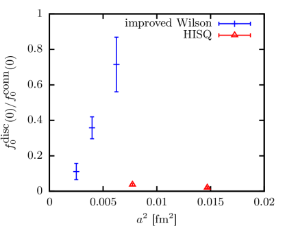
Figure 11: A comparison of the ratio of quark-line disconnected to connected contributions for the $\overline{u}u+\overline{d}d$ current to the pion scalar form factor at $q^{2}=0$ plotted against the square of the lattice spacing. Results denoted by the blue plus symbol for an improved Wilson action are taken from Gülpers et al. (2015). The red triangles are from the results presented here for the HISQ action.

Figure 10 compares our results for our various pion scalar mean square radii to those obtained on $n_{f}=2$ gluon configurations and to the expected values from chiral perturbation theory given above. There is reasonable agreement (within $2\sigma$) between all the lattice QCD results for $\langle r^{2}\rangle^{(\pi)}_{S,ud}$ and with the values expected from $F_{\pi}/F$. Our result for the flavour octet radius is also in good agreement with the value in eq. (25). To illustrate how important the contributions from the disconnected diagrams are to the various scalar radii we also show the result from our calculation of the connected diagram only (eq (11)). As discussed in Section II.2.2 the contributions from the disconnected diagrams to the form factor are small but the change in the slope and therefore in the radius is substantial. This feature of the scalar radius is also discussed in Guelpers et al. (2014); Gülpers et al. (2015).

Our results are in both qualitative agreement and reasonable quantitative agreement with the picture expected from chiral perturbation theory Jüttner (2012). There the disconnected contribution to the form factor is predicted to be very small at $q^{2}=0$, becoming negative at negative $q^{2}$ values so that the contribution to the radius is substantial (approximately equal to that of the connected contribution) and positive. We find the contribution to amount to an approximately 50% increase in the radius, rather than doubling, but with substantial uncertainty.

Although different lattice QCD formalisms will have a different normalisation for the scalar current, the ratio of disconnected to connected contributions to the form factor at a given value of $q^{2}$ should agree in the chiral and continuum limits since renormalisation factors will then cancel. Our results obtained here with the HISQ action seem to agree well with those from the overlap action given at one value of the lattice spacing in Aoki et al. (2009), judging this from their Figure 9. They do not agree well with those from an improved Wilson action given at three values of the lattice spacing in Gülpers et al. (2015). They have a very substantial disconnected contribution that also shows, as a ratio of the connected contribution, a very strong lattice spacing dependence. They work at heavier values of $m_{\pi}$ than we do but see little dependence on $m_{\pi}$ in this ratio (apart from one point that they suggest to treat as an outlier). In Figure 11 we show a comparison of their disconnected/connected ratio at $q^{2}=0$ to ours. For their points we have taken numbers from their Figure 2, using the values closest to $m_{\pi}$ = 250 MeV (so any variation with $m_{\pi}$ is not included in our plot, and it should be taken as an approximate representation of their results). For our results we give values from our coarse set 2 and from fine set 3. Although our results also show some lattice spacing dependence, it is hard to avoid the conclusion that the improved Wilson results are dominated by a lattice artefact. It is not clear whether the values from HISQ/domain wall and improved Wilson actions will agree in the continuum (and chiral) limits and this does need to be resolved.

IV Conclusions

We have given the first lattice QCD results for the vector and scalar form factors of the $\pi$ meson including $u/d$ quarks with their physical masses.

Our results for the vector form factor as a function of $q^{2}$ agree well (needing no extrapolation) with the experimental values from $\pi-e$ scattering (see Figure 3 and eq. (8)). This confirms the encouraging picture seen by earlier lattice QCD calculations (albeit with heavier $u/d$ quark masses and a less realistic QCD vacuum) that lattice QCD does indeed reproduce the QCD effects that result in a finite electric charge radius for the $\pi$ meson. It would clearly be possible to extend our results to higher values of $q^{2}$ with the aim of eventually matching on to expectations from QCD perturbation theory (see, for example, Bonnet et al. (2005)). This would require finer lattices to avoid large discretisation errors from the discretisation of momentum and, for numerical efficiency, should probably be done with heavier-than-physical $\pi$ mesons (even $\eta_{s}$ mesons).

The $\pi$ scalar form factor is of less immediate phenomenological interest but can be stringent test of low-energy expectations from QCD and from chiral perturbation theory (where it can be related to decay constants and $\pi-\pi$ scattering). Here we have given the first results to include $u$, $d$ and $s$ quarks in the sea and in the scalar current. This allows us to define a number of different radii for different flavour combinations. Calculation of the scalar form factor must include the effect of quark-line disconnected diagrams and we agree with earlier results that these have a substantial impact on the determination of the radii. An increase in the radius occurs where $\overline{q}q$ has a positive coefficient in the combination that appears in the scalar current and we find the magnitude of the contribution of $\overline{l}l$ to be larger than that of $\overline{s}s$. We therefore have an ordering in value of the different radii that we give in eq. (20). Our values for the quark-line disconnected contribution to the form factor are, however, very small at $q^{2}=0$ in agreement with expectations from chiral perturbation theory and with earlier results using the overlap formalism Aoki et al. (2009).

Our value for the radius obtained using a $u/d$ scalar current (eq. (18)) agrees within $2\sigma$ with expectations from chiral perturbation theory and earlier values from calculations including $u$ and $d$ quarks in the sea. We give the first results for the radius from the flavour octet and flavour singlet scalar currents (eq. (17)). The flavour octet mean square radius agrees well with expectations from chiral perturbation theory where it can be related to $f_{K}/f_{\pi}$ and combinations of meson masses.

Our largest source of uncertainty in the scalar case is from finite-volume corrections since we are working with physically light $\pi$ mesons, even if on lattices 5.8 fm across. To improve uncertainties on the scalar radius we would need to use larger volumes at the physical point, or include a dedicated study of finite-volume effects away from the physical point, and ensembles of gluon field configurations exist on which this could be done. Improved statistics on the quark-line disconnected contributions are also necessary to reduce the statistical uncertainty in their impact on the scalar mean square radius. The new techniques we have introduced here for handling the disconnected contributions in the pion scalar form factor make these improvements feasible in future results.

Acknowledgements. We are grateful to MILC for the use of their gauge configurations and code and to G. Donald, W. Freeman, V. Gülpers, A. Lytle, D. Toussaint and G. von Hippel for useful discussions. This work was funded by STFC, NSF, the Royal Society and the Wolfson Foundation. We used the Darwin Supercomputer of the University of Cambridge High Performance Computing Service as part of STFC’s DiRAC facility jointly funded by STFC, BIS and the Universities of Cambridge and Glasgow. We are grateful to the Darwin support staff for assistance.

References

- Amendolia et al. (1986) S. Amendolia et al. (NA7 Collaboration), Nucl.Phys. B277, 168 (1986).
- Davies et al. (2004) C. Davies et al. (HPQCD/UKQCD/MILC/Fermilab Lattice Collaborations), Phys.Rev.Lett. 92, 022001 (2004), arXiv:hep-lat/0304004 [hep-lat] .
- Dowdall et al. (2013) R. Dowdall, C. Davies, G. Lepage, and C. McNeile (HPQCD Collaboration), Phys.Rev. D88, 074504 (2013), arXiv:1303.1670 [hep-lat] .
- Gasser and Leutwyler (1984) J. Gasser and H. Leutwyler, Annals Phys. 158, 142 (1984).
- Brommel et al. (2007) D. Brommel et al. (QCDSF/UKQCD Collaboration), Eur.Phys.J. C51, 335 (2007), arXiv:hep-lat/0608021 [hep-lat] .
- Frezzotti et al. (2009) R. Frezzotti, V. Lubicz, and S. Simula (ETM Collaboration), Phys.Rev. D79, 074506 (2009), arXiv:0812.4042 [hep-lat] .
- Brandt et al. (2013) B. B. Brandt, A. Jüttner, and H. Wittig, JHEP 1311, 034 (2013), arXiv:1306.2916 [hep-lat] .
- Aoki et al. (2009) S. Aoki et al. (JLQCD, TWQCD), Phys.Rev. D80, 034508 (2009), arXiv:0905.2465 [hep-lat] .
- Aoki et al. (2015) S. Aoki, G. Cossu, X. Feng, S. Hashimoto, T. Kaneko, J. Noaki, and T. Onogi (JLQCD), (2015), arXiv:1510.06470 [hep-lat] .
- Nguyen et al. (2011) O. H. Nguyen, K.-I. Ishikawa, A. Ukawa, and N. Ukita, JHEP 1104, 122 (2011), arXiv:1102.3652 [hep-lat] .
- Boyle et al. (2008) P. Boyle, J. Flynn, A. Jüttner, C. Kelly, H. P. de Lima, et al., JHEP 0807, 112 (2008), arXiv:0804.3971 [hep-lat] .
- Fukaya et al. (2014) H. Fukaya, S. Aoki, S. Hashimoto, T. Kaneko, H. Matsufuru, et al., Phys.Rev. D90, 034506 (2014), arXiv:1405.4077 [hep-lat] .
- Guelpers et al. (2014) V. Guelpers, G. von Hippel, and H. Wittig, Phys.Rev. D89, 094503 (2014), arXiv:1309.2104 [hep-lat] .
- Gülpers et al. (2015) V. Gülpers, G. von Hippel, and H. Wittig, (2015), arXiv:1507.01749 [hep-lat] .
- Gasser and Leutwyler (1983) J. Gasser and H. Leutwyler, Phys.Lett. B125, 325 (1983).
- Colangelo et al. (2001) G. Colangelo, J. Gasser, and H. Leutwyler, Nucl.Phys. B603, 125 (2001), arXiv:hep-ph/0103088 [hep-ph] .
- Jüttner (2012) A. Jüttner, JHEP 1201, 007 (2012), arXiv:1110.4859 [hep-lat] .
- Follana et al. (2007) E. Follana, Q. Mason, C. Davies, K. Hornbostel, P. Lepage, et al. (HPQCD/UKQCD Collaborations), Phys.Rev. D75, 054502 (2007), arXiv:hep-lat/0610092 [hep-lat] .
- Donald et al. (2012) G. Donald, C. Davies, R. Dowdall, E. Follana, K. Hornbostel, et al. (HPQCD Collaboration), Phys.Rev. D86, 094501 (2012), arXiv:1208.2855 [hep-lat] .
- Bazavov et al. (2010) A. Bazavov et al. (MILC collaboration), Phys.Rev. D82, 074501 (2010), arXiv:1004.0342 [hep-lat] .
- Bazavov et al. (2013) A. Bazavov et al. (MILC Collaboration), Phys.Rev. D87, 054505 (2013), arXiv:1212.4768 [hep-lat] .
- Hart et al. (2009) A. Hart, G. von Hippel, and R. Horgan (HPQCD Collaboration), Phys.Rev. D79, 074008 (2009), arXiv:0812.0503 [hep-lat] .
- Borsanyi et al. (2012) S. Borsanyi, S. Durr, Z. Fodor, C. Hoelbling, S. D. Katz, et al., JHEP 1209, 010 (2012), arXiv:1203.4469 [hep-lat] .
- Draper et al. (1989) T. Draper, R. Woloshyn, W. Wilcox, and K.-F. Liu, Nucl.Phys. B318, 319 (1989).
- Guadagnoli et al. (2006) D. Guadagnoli, F. Mescia, and S. Simula, Phys.Rev. D73, 114504 (2006), arXiv:hep-lat/0512020 [hep-lat] .
- Lepage et al. (2002) G. P. Lepage, B. Clark, C. Davies, K. Hornbostel, et al., Nucl. Phys. Proc. Suppl. 106, 12 (2002), arXiv:hep-lat/0110175 .
- Koponen et al. (2013) J. Koponen, C. Davies, G. Donald, E. Follana, G. Lepage, et al. (HPQCD Collaboration), (2013), arXiv:1305.1462 [hep-lat] .
- Donald et al. (2014) G. Donald, C. Davies, J. Koponen, and G. Lepage (HPQCD Collaboration), Phys.Rev. D90, 074506 (2014), arXiv:1311.6669 [hep-lat] .
- McNeile et al. (2013) C. McNeile, A. Bazavov, C. Davies, R. Dowdall, K. Hornbostel, et al., Phys.Rev. D87, 034503 (2013), arXiv:1211.6577 [hep-lat] .
- Chakraborty et al. (2015) B. Chakraborty, C. Davies, B. Galloway, P. Knecht, J. Koponen, et al. (HPQCD Collaboration), Phys.Rev. D91, 054508 (2015), arXiv:1408.4169 [hep-lat] .
- Aubin et al. (2004) C. Aubin et al. (MILC Collaboration), Phys.Rev. D70, 114501 (2004), arXiv:hep-lat/0407028 [hep-lat] .
- Colquhoun et al. (2015) B. Colquhoun, R. J. Dowdall, J. Koponen, C. T. H. Davies, and G. P. Lepage (HPQCD Collaboration), (2015), arXiv:1510.07446 [hep-lat] .
- Jiang and Tiburzi (2007) F. J. Jiang and B. C. Tiburzi, Phys. Lett. B645, 314 (2007), arXiv:hep-lat/0610103 [hep-lat] .
- Bijnens and Relefors (2014) J. Bijnens and J. Relefors, JHEP 05, 015 (2014), arXiv:1402.1385 [hep-lat] .
- Olive et al. (2014) K. Olive et al. (Particle Data Group), Chin.Phys. C38, 090001 (2014).
- Na et al. (2010) H. Na, C. T. Davies, E. Follana, G. P. Lepage, and J. Shigemitsu (HPQCD Collaboration), Phys.Rev. D82, 114506 (2010), arXiv:1008.4562 [hep-lat] .
- Freeman and Toussaint (2013) W. Freeman and D. Toussaint (MILC), Phys.Rev. D88, 054503 (2013), arXiv:1204.3866 [hep-lat] .
- Kilcup and Sharpe (1987) G. W. Kilcup and S. R. Sharpe, Nucl. Phys. B283, 493 (1987).
- Davies et al. (2010) C. T. H. Davies, E. Follana, I. D. Kendall, G. P. Lepage, and C. McNeile (HPQCD Collaboration), Phys. Rev. D81, 034506 (2010), arXiv:0910.1229 [hep-lat] .
- Freeman and Toussaint (tion) W. Freeman and D. Toussaint, (private communication).
- Liesenfeld et al. (1999) A. Liesenfeld et al. (A1), Phys.Lett. B468, 20 (1999), arXiv:nucl-ex/9911003 [nucl-ex] .
- Quenzer et al. (1978) A. Quenzer, M. Ribes, F. Rumpf, J. Bertrand, J. Bizot, et al., Phys.Lett. B76, 512 (1978).
- Dally et al. (1982) E. Dally, J. Hauptman, J. Kubic, D. Stork, A. Watson, et al., Phys.Rev.Lett. 48, 375 (1982).
- Bebek et al. (1978) C. Bebek, C. Brown, S. D. Holmes, R. Kline, F. Pipkin, et al., Phys.Rev. D17, 1693 (1978).
- Gasser and Leutwyler (1985) J. Gasser and H. Leutwyler, Nucl. Phys. B250, 517 (1985).
- Owen et al. (2015) B. Owen, W. Kamleh, D. Leinweber, B. Menadue, and S. Mahbub, Phys. Rev. D91, 074503 (2015), arXiv:1501.02561 [hep-lat] .
- Aoki et al. (2014) S. Aoki et al., Eur. Phys. J. C74, 2890 (2014), arXiv:1310.8555 [hep-lat] .
- Bonnet et al. (2005) F. D. Bonnet, R. G. Edwards, G. T. Fleming, R. Lewis, and D. G. Richards (Lattice Hadron Physics Collaboration), Phys.Rev. D72, 054506 (2005), arXiv:hep-lat/0411028 [hep-lat] .