The Kuramoto model in complex networks

Abstract

Synchronization of an ensemble of oscillators is an emergent phenomenon present in several complex systems, ranging from social and physical to biological and technological systems. The most successful approach to describe how coherent behavior emerges in these complex systems is given by the paradigmatic Kuramoto model. This model has been traditionally studied in complete graphs. However, besides being intrinsically dynamical, complex systems present very heterogeneous structure, which can be represented as complex networks. This report is dedicated to review main contributions in the field of synchronization in networks of Kuramoto oscillators. In particular, we provide an overview of the impact of network patterns on the local and global dynamics of coupled phase oscillators. We cover many relevant topics, which encompass a description of the most used analytical approaches and the analysis of several numerical results. Furthermore, we discuss recent developments on variations of the Kuramoto model in networks, including the presence of noise and inertia. The rich potential for applications is discussed for special fields in engineering, neuroscience, physics and Earth science. Finally, we conclude by discussing problems that remain open after the last decade of intensive research on the Kuramoto model and point out some promising directions for future research.

List of Abbreviations

BA	Barabási-Albert
CM	configuration model
ER	Erdős-Rényi
FPE	Fokker-Planck equation
FSS	finite-size scaling
GA	Gaussian approximation
MFA	mean-field approximation
MSF	master stability function
OA	Ott-Antonsen
PA	preferential attachment
SF	scale-free
SW	small-world

List of Symbols

$\mathbf{A}$	Adjacency matrix
$\mathcal{A}$	Assortativity
$\mathcal{BS}$	Basin stability
$\alpha$	Damping constant
$\beta$	Critical exponent of the phase transition
$\bar{\nu}$	Finite-size scaling exponent
$cc_{i}$	Local clustering coefficient
$D$	Noise strength
$\sigma^{\rm{A}}$	Adjacency matrix eigenvalues
$\sigma^{\rm{L}}$	Laplacian matrix eigenvalues
$E$	Number of edges
$k$	Degree
$\left\langle k\right\rangle$	Network average degree
$k_{\min}$	Minimum degree
$k_{\max}$	Maximum degree
$P(k)$	Degree distribution
$\mathbf{L}$	Laplacian matrix
$\lambda$	Coupling strength
$\lambda_{c}$	Critical coupling strength
$\lambda_{c}^{\rm{I}}$	Critical coupling strength for increasing coupling branch
$\lambda_{c}^{\rm{D}}$	Critical coupling strength for decreasing coupling branch
$\left\langle\cdot\right\rangle$	Ensemble average
$\left\langle\cdot\right\rangle_{t}$	Temporal average
$N$	Network size
$\nu$	Frequency
$\theta$	Phase
$\phi$	Phase in the rotating frame
$t$	Time
$\omega$	Natural frequency
$g(\omega)$	Natural frequency distribution
$\psi$	Mean phase
$\Omega$	Locking frequency
$R$	Kuramoto order parameter
$r$	Global order parameter accounting the mean-field of uncorrelated networks
$r_{i}$	Local order parameter
$r_{i}^{\rm{T}}$	Local order parameter taking into account time fluctuations.
$r_{\rm{lock}}$	Contribution of locked oscillators to the order parameter
$r_{\rm{drift}}$	Contribution of drifting oscillators to the order parameter
$r^{\rm{D}}$	Order parameter associated to the decreasing branch
$r^{\rm{I}}$	Order parameter associated to the increasing branch
$\tau$	Time delay
$\tau_{r}$	Relaxation time
$\chi$	Susceptibility
$\mathcal{T}$	Transitivity

1 Introduction

Synchronization phenomena are ubiquitous in nature, science, society, and technology. Examples of oscillators are fireflies, lasers, neurons and heart cells [1]. Among the many models proposed for a description of synchronization [1], the Kuramoto model is the most popular nowadays. It describes self-sustained phase oscillators rotating at heterogeneous intrinsic frequencies coupled through the sine of their phase differences. This model exhibits a phase transition at a critical coupling, beyond which a collective behavior is achieved. Since its original formulation 40 years ago [2, 3], several variations, extensions and applications of the Kuramoto model have been documented in the literature. In 2005, Acebrón et al. [4] published the first survey addressing the Kuramoto model, discussing the main works available at that time.

In parallel with the advances in the study of the traditional Kuramoto model, over almost the last two decades one has witnessed the rapid development of the new field of network science [5], which not only brought new insights into the characterization of real networks, but also introduced a new dimension in the study of dynamical systems [6, 7]. Researchers were puzzled by the question of how the connectivity pattern between elements in a network can influence the performance of dynamical processes, such as epidemic spreading, percolation, diffusion, opinion formation and synchronization. This apparently simple question has motivated a lot of studies comprised in several reviews (e.g. [8, 9, 10, 11, 12, 13, 14, 15, 16, 17, 18, 19]) and books (e.g. [20, 21, 22, 23, 24, 25, 26]) on the topic. Curiously, the rise of network science is intimately related to the study of synchronization among coupled oscillators. As described in [20], Watts and Strogatz conceived the idea of including shortcuts between oscillators connected as a regular graph to analyze how crickets synchronize their chirps. It turns out that the simple inclusion of a few shortcuts greatly reduces the average topological distance between the oscillators, improving the synchronous behavior between them [27, 28]. In this way, through this process, the so-called small-world phenomenon was formalized and quantified in the context of networks. This analysis is a milestone in the study of complex systems triggering an overwhelming number of papers. In 2004, the Kuramoto model was generalized to scale-free networks [29] to address the role played by highly connected nodes (hubs) in network dynamics. After that, most of the focusing has mainly aimed at determining how network structure influences the onset of synchronization.

In 2006, Boccaletti et al. [11] provided the first review encompassing structural and dynamical properties of complex networks, where the first theoretical approaches to the Kuramoto model in networks were reviewed. However, the study of the interplay between network structure and dynamics was still in its infancy. In the following years this study rapidly evolved in a way that in 2008 Arenas et al. [14] published a survey in Physics Reports devoted to the analysis of synchronization in networks. The authors focused on two main topics, namely the study of synchronization in the framework of the master stability function (MSF) and networks of Kuramoto oscillators. Regarding the latter subject, significant new analytical and numerical findings were revised, mainly studies on the relation between synchronization and network structure.

However, several important new results on the Kuramoto model have been published since then. In particular, the development of new network models has enabled the study of how different network properties affect synchronization. More specifically, the early works on the Kuramoto model in networks have naturally focused on the influence of topological properties present in the traditional models, such as the presence of shortcuts and hubs. In the last years new classes of random network models that go beyond the reproduction of the degree distribution of real-world networks have been proposed. Basic topological properties such as the occurrence of triangles, emergence of communities, degree-degree correlations and distribution of subgraphs were incorporated in variations of the traditional configuration model allowing the investigation of the effect of these properties on dynamical processes. Not only these non-trivial properties encountered in real networks, but also new types of network representations have been incorporated in the investigations. Namely, in the last couple of years the so-called multilayer networks have been attracting the attention of network researchers and, as we shall see, neglecting the multilayer character can greatly alter the synchronous behavior between the oscillators [17, 18].

It is also important to emphasize that until 2011 only continuous synchronization transitions in the Kuramoto model in networks were reported. The discovery of first-order phase transitions to synchronization (also named as “Explosive Synchronization” [30]) as a consequence of the correlation between structure and local dynamics has triggered several investigations. Moreover, the study of temporal networks, whose structures change in time, has provided new versions of the Kuramoto model. The exploration of several properties in the model, such as the inclusion of stochastic fluctuations, time-delay and repulsive couplings, is also a new tendency in the analysis of the Kuramoto model in networks.

The study of the Kuramoto model in complex networks has also been boosted thanks to findings of new synchronization phenomena, such as the emergence of chimera states in which networks of identical oscillators can split into synchronized and desynchronized subpopulations [31]. The ansatz proposed by E. Ott and T. Antonsen [32, 33], which allows a dimensional reduction to a small number of coupled differential equations, is another recent remarkable result that has attracted the interest of researchers. This ansatz has been receiving great attention since 2008 along with its generalizations to networks of Kuramoto oscillators.

Finally, the Kuramoto model in complex networks has been used in several applications, such as modeling neuronal activity and power grids. In particular, the latter system can be suitably modeled by a second-order Kuramoto model, a fact that motivated many other works aiming at generalizing the model to complex networks. In terms of even large perturbations, the recently proposed concept of basin stability has been proved to deepen insights not only on the stability of real power grids, but also on other dynamical systems [34].

After the survey published in 2008, a large number of papers considering the networked Kuramoto model have been published. Noteworthy, recently Dörfler and Bullo provided a comprehensive survey focused on the control of synchronization of phase oscillators applied to technological networks [35]. However, this survey does not cover the main recent works related to the Kuramoto model. For this reason, it is timely to provide a survey about the Kuramoto model in complex networks to contextualize the fundamental works and enable the advance of the field.

1.1 Outline

This report is organized as follows. We begin our review by analysing important aspects of the Kuramoto model in well-known network models in Sec. 2. There, we discuss the first numerical investigations of the model in complex topologies and also introduce analytical treatments that will be used throughout the text. Finite-size effects and the transient dynamics are also examined. In Section 3 we describe the dynamics of Kuramoto oscillators coupled in networks that mimic typical properties of real-world structures. In particular, we review the works devoted to analyzing the influence of non-vanishing clustering-coefficient, degree-degree correlations and presence of nodes grouped into communities on network synchronization. Effects of time-delay and adaptive couplings are studied in Sec. 4. Section 5 reviews the very recent works on the correlation between natural frequencies and local topology and other conditions that are known to yield discontinuous phase transitions in networks made up of Kuramoto oscillators. Section 6 is concerned with the recent developments on the stochastic Kuramoto model in networks. The second-order Kuramoto is presented in Sec. 7, where we discuss the recently introduced concept of basin stability. Section 8 discusses extensive numerical simulations on the optimization of synchronization in networks. In Sec. 9 we summarize relevant applications of the first- and second-order Kuramoto model in real complex systems, such as power-grids, neuronal systems, networks of semiconductor junctions and seismology. Finally, in Section 10 we present our perspectives and conclusions.

2 First-order Kuramoto on traditional network models

Although the first report on a synchronization phenomenon dates back to Huygens in the 17th century [1], the topic of spontaneous emergence of collective behavior in large populations of oscillators was only brought to higher attention after the work by Wiener [36, 37]. Wiener was interested in the generation of alpha rhythms in the brain and his guess was that this particular phenomenon was somehow related with the same mechanism that yields coherent behavior in other biological systems, such as in the synchronous flash of fireflies. Wiener’s idea was interesting and anticipating, but at the same time too complex to get analytical insights from it. A more promising approach was later developed by Winfree [38, 39], who was the first to properly state the problem of collective synchronization mathematically. He proposed a model of a large population of interacting phase oscillators with distributed natural frequencies. By simulating his model, he found that spontaneous synchronization emerges as a threshold process, a phenomenon akin to a phase transition. His main finding was: if the spread of the frequencies is higher compared to the coupling between the oscillators, then each oscillator would run at its own natural frequency, causing the population to behave incoherently. On the other hand, in case that the coupling is sufficiently strong to overcome the heterogeneity in the frequencies, then the system spontaneously locks into synchrony [38].

Deeply motivated by these results, Kuramoto simplified Winfree’s approach to obtain an analytically tractable model, which at the same time would preserve the fundamental assumptions of having oscillators with distributed frequencies interacting through a collective rhythm produced by the rest of the population. The Kuramoto model consists of a population of $N$ phase oscillators whose evolution is dictated by the governing equations [2, 3]

$$\dot{\theta}_{i}=\omega_{i}+\frac{\lambda}{N}\sum_{j=1}^{N}\sin(\theta_{j}-\theta_{i}),\quad i=1\ldots,N,$$ (1)

where $\theta_{i}$ denotes the phase of the $i$th oscillator, $\lambda$ is the coupling strength and $\omega_{i}$ the natural frequencies, which are distributed according to a given probability density $g(\omega)$. In his original approach, Kuramoto considered $g(\omega)$ to be unimodal and symmetric centered at $\omega=\bar{\omega}$, which can be assumed to be $\bar{\omega}=0$ after a shift. Henceforth, throughout this review, we consider the mean frequency as $\bar{\omega}=0$ to have $g(\omega)=g(-\omega)$, always when the distribution $g(\omega)$ is even and symmetric, without loss of generality. Kuramoto further introduced the order parameter [2, 3]

$$Re^{i\psi(t)}=\frac{1}{N}\sum_{j=1}^{N}e^{i\theta_{j}(t)},$$ (2)

in order to quantify the overall synchrony of the population. This quantity has the interesting interpretation of being the centroid of a set of $N$ points $e^{i\theta_{j}}$ distributed in the unit circle in the complex plane. If the phases are uniformly spread in the range $[0,2\pi]$ then $R\approx 0$ meaning that there is no synchrony among the oscillators. On the other hand, when all the oscillators rotate grouped into a synchronous cluster with the same average phase $\psi(t)$ we have $R\approx 1$. We can rewrite the set of Eqs. 1 using the mean-field quantities $R$ and $\psi$ by multiplying both sides of Eq. 2 by $e^{-i\theta_{i}}$ and equating the imaginary parts to obtain

$$\dot{\theta}_{i}=\omega_{i}+\lambda R\sin(\psi-\theta_{i}).$$ (3)

In this formulation, the phases $\theta_{i}$ seem to evolve independently from each other, but the interaction is actually set through $R$ and $\psi$. Furthermore, note that the effective coupling is now proportional to the order parameter $R$, creating a feedback relation between coupling and synchronization. More specifically, small increments in the order parameter $R$ end up by increasing the effective coupling in Eq. 3 attracting, in this way, more oscillators to the synchronous group. From this process, a self-consistent relation between the phases $\theta_{i}$ and the mean-field is found, i.e. $R$ and $\psi$ will define the evolution of $\theta_{i}$, but at the same time, the phases $\theta_{i}$ self-consistently yield the mean-field through Eq. 2.

In the limit of infinite number of oscillators, the system can be described by the probability density $\rho(\theta,\omega,t)$ so that $\rho(\theta,\omega,t)d\theta$ gives the fraction of oscillators with phase betweeen $\theta$ and $\theta+d\theta$ at time $t$ for a given natural frequency $\omega$. Since $\rho$ is nonnegative and $2\pi-$periodic in $\theta$, we have that it satisfies the normalization condition

$$\int_{-\pi}^{\pi}\rho(\theta,\omega,t)d\theta=1.$$ (4)

Furthermore, the density $\rho$ should obey the continuity equation

$$\frac{\partial\rho}{\partial t}+\frac{\partial}{\partial\theta}(\rho v)=0,$$ (5)

where $v(\theta,\omega,t)=\omega+\lambda R\sin(\psi-\theta)$ is the angular velocity of a given oscillator with phase $\theta$ and natural frequency $\omega$ at time $t$. In the continuum limit, the order parameter $R$ and the average phase $\psi$ defined in Eq. 2 are determined in terms of the probability density $\rho(\theta,\omega,t)$ as

$$Re^{i\psi(t)}=\int_{-\pi}^{\pi}\int_{-\infty}^{\infty}e^{i\theta}\rho(\theta,\omega,t)g(\omega)d\omega d\theta.$$ (6)

Equations 5 and 6 admit the trivial solution $R=0$, which corresponds to the stationary distribution $\rho=1/2\pi$, characterizing the incoherent state. In the partial synchronized state ($0<R<1$), the continuity equation (5) yields in the stationary regime ($\partial\rho/\partial t=0$)

$$\rho(\theta,\omega)=\begin{cases}\delta\left[\theta-\psi-\arcsin\left(\frac{\omega}{\lambda R}\right)\right],&\textrm{ if }|\omega|\leq\lambda R\\ \frac{\sqrt{\omega^{2}-(\lambda R)^{2}}}{2\pi|\omega-\lambda R\sin(\theta-\psi)|}&\textrm{ otherwise.}\end{cases}$$ (7)

The solutions for the stationary distribution assert that in the partial synchronized state the oscillators are divided into two groups. Specifically, those with frequencies $|\omega|\leq\lambda R$ correspond to the oscillators entrained by mean-field, i.e. the oscillators that evolve locked in a common average phase $\psi(t)=\Omega t$, where $\Omega$ is the average frequency of the population. On the other hand, the oscillators with $|\omega|>\lambda R$ (referred as drifting oscillators) rotate incoherently. Inserting the stationary distributions in Eq. 6, one obtains the self-consistent equation for $R$

$$R=\lambda R\int_{-\pi/2}^{\pi/2}\cos^{2}\theta g(\lambda R\sin\theta)d\theta,$$ (8)

where the integral corresponds to the contribution of drifting oscillators vanished due to $g(\omega)=g(-\omega)$ and the symmetry $\rho(\theta+\pi,-\omega)=\rho(\theta,\omega)$. By letting $R\rightarrow 0^{+}$ in Eq. 8, we get

$$\lambda_{c}^{\rm{KM}}=\frac{2}{\pi g(0)},$$ (9)

which is the critical coupling strength for the onset of synchronization firstly obtained by Kuramoto [2, 3]. Moreover, expanding the right-hand side of Eq. 8 in powers of $\lambda R$, given that $g^{\prime\prime}(0)<0$, yields

$$R\sim\sqrt{\frac{-16(\lambda-\lambda_{c})}{\pi\lambda_{c}^{4}g^{\prime\prime}(0)}},$$ (10)

for $\lambda\rightarrow\lambda_{c}$. Thus, near the transition point, the order parameter yields the form $R\sim(\lambda-\lambda_{c})^{\beta}$ with $\beta=1/2$, clearly showing an analogy to a second-order phase transition observed in magnetic systems.

Besides being a timely contribution for the understanding of how synchronization in large populations of mutually coupled oscillators sets in, Kuramoto’s analysis also established a link between mean-field techniques in statistical physics and nonlinear dynamics. However, although undoubtedly brilliant and insightful, his approach was not rigorous and left many questions that puzzled the researchers throughout the following years  [40, 4] making it still matter of fundamental research in recent times  [41, 42, 32, 43, 44, 45, 46].

In parallel with the studies on the traditional Kuramoto model, one has witnessed the emergence of an overwhelming number of works focused on particular effects caused by the introduction of heterogeneous connection patterns, letting the interactions to be no longer only restricted to global coupling. In this section we will analyse the results uncovered for standard network topologies, such as in Erdős-Rényi (ER), scale-free (SF) and small-world (SW) networks. In order to do so, we will firstly discuss the required approximations to analytically treat the problem in uncorrelated networks, i.e. networks in which the degree of connected nodes are not correlated (see Appendix A). Subsequently, we discuss the scaling with the system size and finally we study the relaxation dynamics of the model.

The generalization of the Kuramoto model in complex networks is obtained by including the connectivity in the coupling term as [14, 47]

$$\dot{\theta}_{i}=\omega_{i}+\sum_{j=1}^{N}\lambda_{ij}A_{ij}\sin(\theta_{j}-\theta_{i}),$$ (11)

where $\lambda_{ij}$ is the coupling strength between nodes $i$ and $j$ and $A_{ij}$ the elements of the adjacency matrix $\mathbf{A}$ ($A_{ij}=1$ if the re is a connection between nodes $i$ and $j$, or $A_{ij}=0$, otherwise). The definition of the model in Eq. 11 already brings the first problem when treating the model in complex topologies: the choice of $\lambda_{ij}$. In the fully connected graph the coupling $\lambda_{ij}=\lambda/N$ is adopted so that the model is well behaved in the thermodynamic limit $N\rightarrow\infty$, since in this case the connectivity of each oscillators grows linearly with the system size. Thus, the normalization factor for the coupling strength in networks should be defined in a way to incorporate the same scaling observed in the dependence of the connectivity of the nodes on the system size. However, different network models generate different scalings, which make the choice for an intensive coupling $\lambda_{ij}$ to be not unique. This led many researchers to simply adopt a constant coupling $\lambda_{ij}=\lambda$ $\forall i,j$ without any dependence on $N$, i.e. [14]

$$\dot{\theta}_{i}=\omega_{i}+\lambda\sum_{j=1}^{N}A_{ij}\sin(\theta_{j}-\theta_{i}).$$ (12)

Setting the interaction between the oscillators to be through a constant coupling strength without any further normalization factor seems to be more appropriate when comparing the synchronization of different networks, since the total number of connections can scale differently with the network size, depending on the topology considered. The choice for an intensive coupling is indeed an important issue regarding the formulation of the Kuramoto model in complex networks, specially when concerning the determination of the onset of synchronization. Arenas et al. [14] provide an interesting discussion about the different prescriptions for intensive couplings and also the corresponding consequences of each choice in the network dynamics. Here we discuss the results with the normalization terms used in the original papers, commenting, when possible, the limiting cases of different definitions for the coupling strength $\lambda_{ij}$.

2.1 Early works

The first works on the Kuramoto model in complex networks aimed at quantifying the influence of the SW phenomenon on the overall network synchronization [27, 48, 29, 49]. This issue was systematically investigated in [48] by considering oscillators with natural frequencies distributed according to a Gaussian distribution coupled in SW networks originated from one-dimensional regular lattices. By numerically evolving the equations (11) with $\lambda_{ij}=\lambda/\left\langle k\right\rangle$ in order to obtain the dependence of the order parameter $R$ (Eq. 2) on the coupling strength for different values of the rewiring probability $p$ (see Appendix A), it was found that a small percentage of shortcuts is able to dramatically improve network synchronization in comparison to the completely regular case. Interestingly, this enhancement in the coherence between the oscillators was verified to saturate for intermediate values of the rewiring probability (see Fig. 1). In other words, for $p\gtrsim 0.5$, the synchronization of SW networks exhibit no significant difference than the fully random case ($p=1$). This shows that, in an application context where the optimization of the network synchronization is sought, no improvement in the collective behavior between oscillators is obtained beyond a critical value of the rewiring probability, leading to a save of resources in cases in which rewirings have costs associated.

These results thus suggest that the critical coupling $\lambda_{c}$ for the onset of synchronization should be a decreasing function of $p$. However, to thoroughly evaluate this dependence, finite-size effects should be taken into account. The order parameter was then proposed to take the usual scaling form as [48, 50]

$$R=N^{-\frac{\beta}{\bar{\nu}}}F\left[(\lambda-\lambda_{c})N^{\frac{1}{\bar{\nu}}}\right],$$ (13)

where $F\left[\cdot\right]$ is a scaling function. At $\lambda=\lambda_{c}$ the function $F$ becomes independent of $N$ and, by plotting $RN^{\beta/\bar{\nu}}$ for different values of $N$, the ratio $\beta/\bar{\nu}$ is then determined by the value that yields the best matching between the curves at $\lambda_{c}$. Once $\beta/\bar{\nu}$ is calculated, one can determine $\bar{\nu}$ through

$$\ln\left[\left.\frac{dR}{d\lambda}\right|_{\lambda_{c}}\right]=\frac{1-\beta}{\bar{\nu}}\ln N+\mbox{const},$$ (14)

which together with $\beta/\bar{\nu}$ gives the exponents $\beta$ and $\bar{\nu}$. Despite the sparse number of connections, the dynamics in SW networks apparently exhibited the same scaling with the system size as the model in the fully connected graph [51], namely with $\beta\sim 1/2$ and $\bar{\nu}\sim 2$, and consequently the same mean-field character of the scaling near the critical coupling $R\sim(\lambda-\lambda_{c})^{\beta}$ [48]. However, new results on the finite-size scaling (FSS) of Kuramoto model in the fully connected graph [52, 53] and in SW networks [54] verified that the correct critical exponent should be $\bar{\nu}=5/2$ instead of $\bar{\nu}=2$ for both topologies (see also [55] for results on the FSS of directed SW networks). We shall discuss finite-size effects in more details in Sec. 2.2.

Figure 1: Order parameter $R$ (Eq. 2) as a function of coupling $\lambda$ of SW networks with different values of the rewiring probability $p$. GL and AN stand for globally coupled network and its respective analytical solution, respectively. Adapted with permission from [48]. Copyrighted by the American Physical Society.

Moreno and Pacheco addressed the same questions for SF networks generated by the Barabási-Albert (BA) model (see Appendix A) [29] with uniform frequency distributions. Surprisingly, a similar dependence of the order parameter $R$ on the coupling strength $\lambda$ was verified. In fact, the obtained critical exponent, $\beta\sim 0.46$, suggested that SF networks also exhibit the same square-root behavior of the mean-field synchronization transition observed in the standard Kuramoto model [29]. Interestingly, the same choice of uniform frequency distribution is known to yield a discontinuity in the order parameter as a function of coupling $\lambda$ in the fully connected graph [56] (see Sec. 5), in striking contrast with the result in SF networks [29].

The first numerical results left many questions to be solved regarding the onset of synchronization specially due to the finite value of the critical coupling $\lambda_{c}$ found in SF networks [29, 14]. The reason for this unexpected behavior resides in the fact that critical properties of other dynamical processes, such as epidemic spreading and percolation, were predicted to vanish as a consequence of the high degree of heterogeneity found in these networks [47].

In contrast with the formulation in the fully connected graph, the Kuramoto model has no exact solution in heterogeneous networks. Unfortunately, in the latter case, the system of equations (12) cannot be exactly decoupled by a global mean-field as in Eq. 3 and approximations need to be considered.

Before presenting the most adopted mean-field approach, let us first discuss the so-called time-average approximation. Restrepo et al. [57] defined a local order parameter in a way to take explicitly into account the contribution of time fluctuations. More specifically, the local mean-field of the neighborhood of node $i$ is given by [57, 58]

$$r_{i}^{\rm{T}}e^{i\psi_{i}}=\sum_{j=1}^{N}A_{ij}\left\langle e^{i\theta_{j}}\right\rangle_{t},$$ (15)

where $\left\langle\cdots\right\rangle_{t}$ is a time average. Using Eq. 15, it is possible to write Eq. 12 as

$$\dot{\theta}_{i}=\omega_{i}+\lambda r_{i}^{\rm{T}}\sin(\psi_{i}-\theta_{i})-\lambda h_{i}(t),$$ (16)

where $h_{i}(t)=\textrm{Im}\{e^{-i\theta_{i}}\sum_{j=1}^{N}A_{ij}(\left\langle e^{i\theta_{j}}\right\rangle_{t}-e^{i\theta_{j}})\}$ is the term that evaluates the contribution of time fluctuations. Beyond the onset of synchronization it is expected that the oscillators are locked in a common phase making the order parameter to be of order $r_{i}^{\rm{T}}\sim k_{i}$. Since $h_{i}(t)$ is a sum of independent terms we then expect $h_{i}(t)\sim\sqrt{k_{i}}$ [57]. Thus, for networks in the limit of large average degrees, the term $h_{i}(t)$ can be neglected in comparison with the magnitude of $r_{i}^{\rm{T}}$ leading to

$$\dot{\theta}_{i}=\omega_{i}+\lambda r_{i}^{\rm{T}}\sin(\psi_{i}-\theta_{i}).$$ (17)

In the time-independent regime $\dot{\theta}_{i}=0$, the locked oscillators have their phases given by $\sin(\theta_{i}-\psi_{i})=\omega_{i}/\lambda r_{i}^{\rm{T}}$. In this way, the order parameter (15) can be written as

$$r_{i}^{\rm{T}}=\sum_{j=1}^{N}A_{ij}\langle e^{i(\theta_{j}-\psi_{i})}\rangle_{t}=\sum_{|\omega_{j}|\leq\lambda r_{j}^{\rm{T}}}A_{ij}e^{i(\theta_{j}-\psi_{i})}+\sum_{|\omega_{j}|>\lambda r_{j}^{\rm{T}}}A_{ij}\langle e^{i(\theta_{j}-\psi_{i})}\rangle_{t},$$ (18)

where the two terms above stand for the contribution of synchronous and drifting oscillators, respectively. The latter can be computed by noting that the time average in Eq. 18 is given by [57]

$$\langle e^{i\theta_{j}}\rangle_{t}=\int_{-\pi}^{\pi}\rho(\theta|\omega_{j},r_{j}^{\rm{T}})d\theta,$$ (19)

where $\rho(\theta|\omega_{j},r_{j}^{\rm{T}})d\theta$ is the probability of finding the phase $\theta_{j}$ between $\theta$ and $\theta+d\theta$ for a given $\omega_{j}$ and $r_{j}^{\rm{T}}$. As $\rho\sim 1/|\dot{\theta}|$ we have that

$$\rho(\theta|\omega_{j},r_{j}^{\rm{T}})=\frac{\sqrt{\omega_{j}^{2}-\lambda^{2}(r_{j}^{\rm{T}})^{2}}}{2\pi|\omega_{j}+\lambda r_{j}^{{\rm T}}\sin(\psi_{j}-\theta)|}.$$ (20)

Using Eq. 20 and 19 we obtain the contribution of drifting oscillators, i.e.

$$\sum_{|\omega_{j}|>\lambda r_{j}^{\rm{T}}}A_{ij}\langle e^{i\theta_{j}}\rangle_{t} = \sum_{|\omega_{j}|>\lambda r_{j}^{\rm{T}}}A_{ij}\lambda r_{j}^{\rm{T}}\sqrt{\omega_{j}^{2}-\lambda(r_{j}^{\rm{T}})^{2}}{\rm sgn}(\omega_{j})\frac{1}{2\pi}$$

$$\times\int_{-\pi}^{\pi}\frac{e^{i\theta}\sin(\theta-\psi_{j})d\theta}{\omega_{j}^{2}-\lambda^{2}(r_{j}^{\rm{T}})^{2}\sin^{2}(\theta-\psi_{j})}$$

Assuming that the variables $r_{i}^{\rm{T}}$, $\psi_{i}$ and $\omega_{i}$ are statistically independent and considering that the frequency distribution $g(\omega)$ is symmetric, we have that summation in Eq. 2.1 is of the order $\sqrt{k_{i}}$ and can be neglected in comparison with the contribution of locked oscillators [57]. Under these conditions Eq. 18 is reduced to

$$r_{i}^{\rm{T}}=\sum_{|\omega_{j}|\leq\lambda r_{j}^{\rm{T}}}A_{ij}\cos(\psi_{j}-\psi_{i})\sqrt{1-\left(\frac{\omega_{j}}{\lambda r_{j}^{\rm{T}}}\right)^{2}}$$ (21)

The previous self-consistent equation for the order parameter $r_{i}^{\rm{T}}$ is valid if the onset of synchronization is reached, i.e., for $\lambda>\lambda_{c}$. Furthermore, the minimal value for $\lambda_{c}$ is obtained for $\cos(\psi_{i}-\psi_{j})=1$, which yields [57]

$$r_{i}^{\rm{T}}=\sum_{|\omega_{j}|\leq\lambda r_{j}^{\rm{T}}}A_{ij}\sqrt{1-\left(\frac{\omega_{j}}{\lambda r_{j}^{\rm{T}}}\right)^{2}}$$ (22)

Thus, once the adjacency matrix $\mathbf{A}$ and the natural frequencies $\omega_{i}$ of the whole population are known, Eq. 22 can be numerically solved in order to obtain the dependence of $r_{i}^{\rm{T}}$ on $\lambda$. Since the time fluctuations can be neglected for connected networks with sufficient large average degrees, from now on we abandon the upper script and the time average in Eq. 15 and define the local order parameter simply by $r_{i}e^{i\psi_{i}(t)}=\sum_{j=1}^{N}A_{ij}e^{i\theta_{j}(t)}$. In this formulation, the overall network synchronization can be quantified through averaging the local order parameters $r_{i}$ as [57]

$$z=re^{i\psi(t)}=\frac{\sum_{j=1}^{N}r_{j}}{\sum_{j=1}^{N}k_{j}}.$$ (23)

Suppose now that the oscillators are not described by a particular sequence of natural frequencies but rather by frequencies distributed according to some function $g(\omega)$. Then, Eq. 22 can be formulated as

$$r_{i}=\sum_{j}A_{ij}\int_{-\lambda r_{j}}^{\lambda r_{j}}g(\omega)\sqrt{1-\left(\frac{\omega}{\lambda r_{j}}\right)^{2}}d\omega=\lambda\sum_{j}A_{ij}r_{j}\int_{-1}^{1}g(x\lambda r_{j})\sqrt{1-x^{2}}dx,$$ (24)

where $x=\omega/\lambda r_{j}$. Equation 24 is also known as the frequency approximation [57]. Near the onset of synchronization, $r_{j}\rightarrow 0^{+}$, one can use the first-order approximation $g(x\lambda r_{j})\approx g(0)$ to obtain

$$r_{j}^{(0)}=\frac{\lambda}{\lambda^{\rm{KM}}_{c}}\sum_{j=1}^{N}A_{ij}r_{j}^{(0)}.$$ (25)

The smallest value of $\lambda$ that satisfies the previous equations is precisely the critical coupling $\lambda_{c}$, which is identified to be dependent on the largest eigenvalue $\sigma_{\max}^{\rm{A}}$ of $\mathbf{A}$ [57]:

$$\lambda_{c}=\frac{\lambda_{c}^{\rm{KM}}}{\sigma_{\max}^{\rm{A}}}.$$ (26)

This result can be complemented by the estimation of $\sigma_{\max}^{\rm{A}}$ for different network models. In particular, for uncorrelated networks with a given degree distribution we have that [59]

$$\sigma_{\max}^{\rm{A}}\sim\begin{cases}\frac{\left\langle k^{2}\right\rangle}{\left\langle k\right\rangle}&\textrm{{\rm if }}\frac{\left\langle k^{2}\right\rangle}{\left\langle k\right\rangle}>\sqrt{k_{\max}}\ln N\\ \sqrt{k_{\max}}&\textrm{{\rm if }}\sqrt{k_{\max}}>\frac{\left\langle k^{2}\right\rangle}{\left\langle k\right\rangle}\ln^{2}N,\end{cases}$$ (27)

where $k_{\max}$ is the network largest degree. Note that the critical coupling $\lambda_{c}$ in Eq. 26 takes naturally into account the finite size $N$ of the network. For this reason, although it provides accurate results for the critical coupling in cases where other approaches fail [57], Eq. 26 predicts a vanishing onset of synchronization in the thermodynamic limit of SF networks. For instance, for networks with $P(k)\sim k^{-\gamma}$ with $\gamma\leq 3$, the largest degree scales with system size as $k_{\max}\sim N^{1/(\gamma-1)}$, making $\sigma_{\max}^{\rm{A}}\sim N^{1/2(\gamma-1)}$, which diverges for $N\rightarrow\infty$ and thus leading to the well-known result of vanishing $\lambda_{c}\rightarrow 0$, where no phase transition is expected  [60, 57, 14]. This is also true for SF networks with $\gamma>3$. Specifically, in this case, for sufficient large $N$, the largest eigenvalue will almost surely scale as $\sigma_{\max}^{\rm{A}}\sim\sqrt{k_{\max}}$, which also diverges in the limit $N\rightarrow\infty$ predicting, in this way, the absence of a critical coupling for the onset of synchronization. In contrast to Eq. 26, the critical coupling predicted using the mean-field approximation (MFA) remains finite for SF networks with $\gamma>3$, as we shall soon discuss.

Equation 24 can be further explored in order to obtain the dependence of the order parameter near the critical point. A second-order expansion of the term $g(x\lambda rk_{j})$ gives

$$r_{i}=\lambda\sum_{j=1}^{N}A_{ij}r_{j}\int_{-1}^{1}\left(g(0)+\frac{1}{2}g^{\prime\prime}(0)(x\lambda r_{j})^{2}\right)\sqrt{1-x^{2}}dx.$$ (28)

By considering perturbations in the local order parameter in the previous equation, it follows that for $\lambda\rightarrow\lambda_{c}$ the total order parameter $r$ defined in Eq. 23 is given by [57]

$$r^{2}=\left(\frac{\eta_{1}}{c(\lambda_{c}^{{\rm KM}})^{2}}\right)\left(\frac{\lambda}{\lambda_{c}}-1\right)\left(\frac{\lambda}{\lambda_{c}}\right)^{-3},$$ (29)

where $c=-\pi g^{\prime\prime}(0)\lambda_{c}^{\rm{KM}}/16$ and

$$\eta_{1}=\frac{\left\langle\upsilon\right\rangle^{2}(\sigma_{\max}^{\rm{A}})^{2}}{N\left\langle k\right\rangle^{2}\left\langle\upsilon^{4}\right\rangle},$$ (30)

with $\upsilon$ being the normalized eigenvector associated to $\sigma_{\max}^{\rm{A}}$ of $\mathbf{A}$.

One of the most employed approach in the analytical treatment of dynamical processes in networks is to consider MFAs [47, 61]. Such an approximation scheme relies on the assumption that the dynamical state of a given node $i$ depends on a global common field that is equally felt by all individuals in the network. This is translated in the dynamics of the Kuramoto model in networks by considering that the oscillators interact through a global field $re^{i\psi}$ that is related with the local mean-field $r_{j}e^{i\psi_{j}(t)}$ as

$$re^{i\psi}=\frac{1}{k_{j}}r_{j}e^{i\psi_{j}}=\frac{1}{k_{j}}\sum_{j=1}^{N}A_{ij}e^{i\theta_{j}},$$ (31)

i.e., Eq. 31 basically states that the local mean-field felt by a node should be proportional to a global mean-field weighted by the local connectivity, i.e. $r_{j}=rk_{j}$. This assumption is reasonable to be adopted only if the network is well connected (sufficient large average degree) without the presence of communities, i.e. a portion of the network that is more connected within itself than with the other nodes [14, 57]. Using this approximation for the local order parameter the equations governing the phases evolution are decoupled as

$$\dot{\theta}_{i}=\omega_{i}+\lambda rk_{i}\sin(\psi-\theta_{i}).$$ (32)

Note that the effective coupling of node $i$ has a term proportional to its local topology, in contrast with the case of the fully connected graph. For this reason the effects of the network topology on dynamics can be hidden if the coupling strength in Eq. 11 is chosen as $\lambda_{ij}=\lambda/k_{i}$, where the normalization by the degree neutralizes the heterogeneity in the field initially imposed by the network topology [14]. It is interesting to remark that the MFA in Eq. 31 is precisely identical to the so-called annealed network approximation [61]. There, one substitutes $A_{ij}$ by its expected value over an ensemble average of uncorrelated networks with a given degree sequence $\{k_{i}\}$, $i=1,...,N$. In other words, the original problem of a network defined by the adjacency matrix $A_{ij}$ is now mapped into fully connected weighted network described by the adjacency matrix $\tilde{\mathbf{A}}$ with

$$\tilde{A}_{ij}=\frac{k_{i}k_{j}}{N\left\langle k\right\rangle}.$$ (33)

Noteworthy, $\tilde{A}_{ij}$ is also the probability in the configuration model that nodes $i$ and $j$ are connected [25]. Replacing $A_{ij}$ by $\tilde{A}_{ij}$ in Eq. 12 we get

$$\dot{\theta}_{i}=\omega_{i}+\lambda k_{i}\sum_{j=1}^{N}\frac{k_{j}}{N\left\langle k\right\rangle}\sin(\theta_{j}-\theta_{i}).$$ (34)

In order to decouple Eqs. 34, this formulation motivates the following definition of the global order parameter:

$$re^{\psi(t)}=\frac{1}{N\left\langle k\right\rangle}\sum_{j=1}^{N}k_{j}e^{i\theta_{j}(t)},$$ (35)

which is equivalent to the original definition for the MFA in Eq. 31 and leads precisely to the same set of equations as in (32).

After this detour to show the equivalence of different treatments, let us return to the analysis of Eq. 24 in the frequency approximation scheme. Applying the MFA to $r_{j}$ and summing over $i$ in both sides in Eq. 24 we obtain [60, 57, 62]

$$\sum_{j=1}^{N}k_{j}=\lambda\sum_{j=1}^{N}k_{j}^{2}\int_{-1}^{1}g(x\lambda rk_{j})\sqrt{1-x^{2}}dx.$$ (36)

Tending $r\rightarrow 0^{+}$ one finally gets $\lambda_{c}$ within the MFA

$$\lambda_{c}=\lambda_{c}^{\rm{KM}}\frac{\left\langle k\right\rangle}{\left\langle k^{2}\right\rangle}.$$ (37)

This equation is one of the most known results related to the dynamics of Kuramoto oscillators in networks. It asserts that the value of the critical coupling for the onset of synchronization in the fully connected graph is rescaled by the ratio $\left\langle k\right\rangle/\langle k^{2}\rangle$ of the first two moments of the degree distribution $P(k)$. Therefore, according to Eq. 37, the more heterogeneous the network, the weaker the coupling strength required to synchronize its oscillators. This highlights the role played by the hubs in network dynamics acting improving the overall collective behavior. Furthermore, in contrast to $\lambda_{c}$ predicted by the frequency approximation (Eq. 26), the mean-field scheme gives a finite $\lambda_{c}$ for SF networks with $\gamma>3$ in the thermodynamic limit $N\rightarrow\infty$, in agreement with simulations of sufficient large networks [29, 14]. However, problems arise for more heterogeneous networks with $2<\gamma<3$. In principle, one would expect partial synchronization to emerge for any $\lambda>0$, since $\left\langle k^{2}\right\rangle\rightarrow\infty$ for this range of $\gamma$. However, as extensive simulations show [14], that seems to be not the case even if the finite number of nodes is taken into account in the estimation of $\lambda_{c}$ using Eq. 37. More specifically, for $\gamma=3$, the second moment of the degree distribution scales with the system size as $\left\langle k^{2}\right\rangle\sim\ln N$, leading to $\lambda_{c}\sim 1/\ln N$  [61, 14, 63]. Although a very high number of oscillators is indeed a limiting factor, simulations with reasonably large networks already present discrepancies with this estimative of $\lambda_{c}$. As previously mentioned, evidences show that in fact $\lambda_{c}$ for SF networks with $2\leq\gamma\leq 3$ seems to converge to a constant value as the system size $N$ is increased, in striking contrast with the prediction of the MFA. Therefore, the question left is what is the source of the disagreement between the result predicted in Eq. 37 and the results observed in simulations. Much has been conjectured about this puzzle [14, 47, 61, 63] but the problem remains open.

Nevertheless, despite the inconsistency in determining $\lambda_{c}$ in the limit of large $N$, further developments can be made using the MFA. Similarly as before, one can expand $g(x\lambda rk_{j})\approx g(0)+\frac{1}{2}g^{\prime\prime}(0)(x\lambda rk_{j})^{2}$ to get

$$r^{2}=\left(\frac{\eta_{2}}{c(\lambda_{c}^{{\rm KM}})^{2}}\right)\left(\frac{\lambda}{\lambda_{c}}-1\right)\left(\frac{\lambda}{\lambda_{c}}\right)^{-3},$$ (38)

where

$$\eta_{2}=\frac{\left\langle k^{2}\right\rangle^{3}}{\left\langle k^{4}\right\rangle\left\langle k\right\rangle^{2}},$$ (39)

which holds once $\left\langle k^{4}\right\rangle$ remains finite [57].

The mean-field result for $\lambda_{c}$ (Eq. 37) was firstly obtained by Ichinomiya [60] using the continuum limit of Eqs. 12. Similarly as considered in the original approach of Kuramoto, in the limit $N\rightarrow\infty$, the population of oscillators can be described by the density $\rho(\theta,t|\omega,k)$ of oscillators that have phase $\theta$ at time $t$ for a given frequency $\omega$ and degree $k$. It is further assumed that, for a given $\omega$ and $k$, $\rho(\theta,t|\omega,k)$ is normalized as

$$\int_{0}^{2\pi}\rho(\theta,t|\omega,k)d\theta=1.$$ (40)

Considering an uncorrelated network with a given degree distribution $P(k)$, the probability that a randomly selected edge has at its end a node with phase $\theta$ at time $t$ for a given degree $k$ and frequency $\omega$ is given by

$$\frac{kP(k)}{\left\langle k\right\rangle}g(\omega)\rho(\theta,t|\omega,k).$$ (41)

The equations for the phases evolution in the continuum limit are then obtained by replacing the sum by the average using Eq. 41 in the right-hand side of Eq. 12, i.e.  [60]

$$\dot{\theta}=\omega+\frac{\lambda k}{\left\langle k\right\rangle}\int d\omega^{\prime}\int dk^{\prime}\int d\theta^{\prime}g(\omega^{\prime})P(k^{\prime})k^{\prime}\rho(\theta^{\prime},t|\omega^{\prime},k^{\prime})\sin(\theta^{\prime}-\theta),$$ (42)

where now the network dynamics is described by the average phases $\theta(t)$. In order to decouple Eqs. 42 one can define the global order parameter as

$$re^{i\psi(t)}=\frac{1}{\left\langle k\right\rangle}\int d\omega\int dk\int d\theta P(k)kg(\omega)\rho(\theta,t|\omega,k)e^{i\theta(t)}.$$ (43)

Note that Eq. 43 is exactly the continuum limit version of the order parameter introduced in the annealed network approximation (Eq. 35). Writing Eq. 43 in terms of the order parameter in the continuum limit, distribution $\rho(\theta,t|\omega,k)$ should then obey the continuity equation

$$\frac{\partial\rho(\theta,t|\omega,k)}{\partial t}=-\frac{\partial}{\partial\theta}\left\{\rho(\theta,t|\omega,k)\left[\omega+\lambda kr\sin(\psi-\theta)\right]\right\},$$ (44)

whose solutions in the stationary regime assuming $\psi=0$, without loss of generality, are given by

$$\rho(\theta|\omega,k)=\begin{cases}\delta\left[\theta-\arcsin\left(\frac{\omega}{\lambda kr}\right)\right]&\mbox{if }\left|\omega\right|\leq\lambda kr\\ \frac{C(\omega,k)}{\left|\omega-\lambda kr\sin\theta\right|}&\mbox{otherwise,}\end{cases},$$ (45)

where $C(\omega,k)=\sqrt{\omega^{2}-(\lambda kr)^{2}}/2\pi$ and $\delta(\cdot)$ is the Dirac delta function. The first and second terms correspond to the density of synchronous and drifting oscillators, respectively. In particular, the latter corresponds to the distribution of drifting oscillators in Eq. 20 formulated in terms of the phases $\theta(t)$. Substituting Eq. 45 in Eq. 43 one gets [60]

$$\int dkP(k)k=\lambda\int dkP(k)k^{2}\int_{-1}^{1}dxg(x\lambda rk)\sqrt{1-x^{2}},$$ (46)

which tending $r\rightarrow 0^{+}$ leads to the same critical coupling obtained in Eq. 37.

The comparison of the aforementioned approximations with simulations is shown in Fig. 2 by plotting $r^{2}$ as a function of $\lambda/\lambda_{c}$ for SF networks with different $\gamma$. As we can see, the time-averaged approximation provides the best agreement with the simulation results for all $\gamma$ considered in Fig. 2. Furthermore, the mean-field technique completely fails to determine the onset of synchronization in networks with $\gamma=2$ (Fig. 2(a)) and $2.5$ (Fig. 2(b)), clearly showing the limitations of such an approximation in highly heterogeneous networks. On the other hand, for more homogeneous networks, as for $\gamma=4$ (Fig. 2(d)), the mean-field solution approaches the results provided by the frequency distribution approximation, which are in better agreement with the simulations.

Figure 2: Comparison of order parameter $r^{2}$ obtained from simulations and theory for SF networks with power-law exponent (a) $\gamma=2$, (b) $\gamma=2.5$, (c) $\gamma=3$ and (d) $\gamma=4$. In all cases the degrees are bounded as $50\leq k\leq 2000$ [57]. TAT, FDA and MF stand for time-average theory (Eq. 22), frequency distribution approximation (Eq. 24) and mean-field (Eq. 38), respectively. Adapted with permission from [57]. Copyrighted by the American Physical Society.

So far we analyzed the onset of synchronization in networks in which the oscillators are symmetrically coupled. A natural and interesting question would then be how the network dynamics is affected by the introduction of asymmetric interactions. Given an undirected network, one way to introduce asymmetry in the couplings between the oscillators is to consider normalization factors in $\lambda_{ij}$ in Eq. 11 that depend on local topological properties of node $i$. This scenario was investigated in [64], as follows

$$\dot{\theta}_{i}=\omega_{i}+\frac{\lambda}{k_{i}^{1-\eta}}\sum_{j=1}^{N}A_{ij}\sin(\theta_{j}-\theta_{i}).$$ (47)

Rewriting the equations in terms of $r$ in the MFA we get

$$\dot{\theta}_{i}=\omega_{i}+\lambda k_{i}^{\eta}r\sin(\psi-\theta_{i}).$$ (48)

In SF networks the coupling $\lambda_{ij}=\lambda/k_{i}^{1-\eta}$ has the interesting property of tuning the influence of hubs on the network dynamics. More specifically, depending on the choice of $\eta$, the contribution of high degree nodes to the heterogeneous mean-field can significantly change the onset of synchronization. By developing an analogous self-consistent analysis within the MFA as in Eq. 36, the effect of $\eta$ on the network dynamics can be summarized by calculating the $\lambda_{c}$, which assumes the following forms [64]

$$\lambda_{c}=\begin{cases}\lambda_{c}^{{\rm KM}}\frac{\left\langle k\right\rangle}{\left\langle k^{1+\eta}\right\rangle}&\textrm{ if }\gamma>3\eta+2\\ \lambda_{c}^{{\rm KM}}\frac{\zeta(\gamma-1)}{\zeta(\gamma-\eta-1)}&\textrm{ if }\eta+2<\gamma<3\eta+2\\ \sim N^{(\eta-\gamma+2)/(\gamma-1)}&\textrm{ if }\eta+1<\gamma<\eta+2,\end{cases}$$ (49)

where $\zeta$ is the Hurwitz zeta function. For $\eta=1$ we recover the symmetric coupling case for which the MFA predicts $\lambda_{c}\rightarrow 0$ in the thermodynamic limit for networks with $2<\gamma<3$. For a general $\eta$, the regime in which $\lambda_{c}$ is expected to vanish is obtained for SF networks in the range $\eta+1<\gamma<\eta+2$. On the other hand, for $\gamma>\eta+2$, $\lambda_{c}$ remains finite as $N\rightarrow\infty$. Note that $\eta=0$ in Eq. 49 completely removes the dependence of $\lambda_{c}$ on the network topology, since it leads to the coupling normalization $\lambda_{ij}=\lambda/k_{i}$ as previously discussed.

One can further show that the nature of the phase synchronization transition crucially depends on the exponent $\eta$. More specifically, near the onset of synchronization, $r\sim(\lambda-\lambda_{c})^{\beta}$, with $\beta$ given by

$$\beta=\begin{cases}\frac{1}{2}&\textrm{ if }\gamma>3\eta+2\\ \eta/(\gamma-2-\eta)&\textrm{ if }\eta+2<\gamma<3\eta+2\\ \eta/(\eta-\gamma+2)&\textrm{ if }\eta+1<\gamma<\eta+2\\ (\gamma-1)/(\eta-\gamma+2)&\textrm{ if }\gamma<\eta+1\end{cases}.$$ (50)

The result above generalizes the scaling of $r$ for different exponents $\eta$. More specifically, in the absence of a normalization factor ($\eta=1$), the mean-field transition with $\beta=1/2$ is only obtained for SF networks with $\gamma=5$. However, by decreasing $\eta$, one obtains mean-field transitions with $\beta=1/2$ for broader degree distributions, a fact that shows how $\eta$ acts on the network dynamics by attenuating the effect of hubs.

2.2 Finite-size effects

We discussed the main early contributions to the theoretical analysis of the Kuramoto model networks, including the approximations used to obtain the dependence of the order parameter on the coupling strength and the related critical exponents. However, the numerical determination of $\lambda_{c}$ essentially relies on simulations of networks that are inherently consisted of a finite number of oscillators. Therefore, the effects of such a limitation should be considered in the analysis. Furthermore, as we shall see, another important feature should be considered for the correct estimation of the critical exponents of the phase transition, namely the sample-to-sample fluctuations generated by different realizations of random natural frequencies as well as randomness introduced by fluctuations in the network topology.

We begin by first analyzing the scaling of the $r$ in uncorrelated SF networks following closely [65]. Considering that the natural frequencies are distributed by a unimodal and even distribution $g(\omega)$, it is convenient to write the self-consistent mean-field equation for $r$ in the symbolic form $r=\widetilde{\mathcal{R}}(\lambda r)$, with

$$\widetilde{\mathcal{R}}(\lambda r)\equiv\frac{1}{N}\sum_{|\omega_{j}|\leq k_{j}\lambda r}\frac{k_{j}}{\left\langle k\right\rangle}\sqrt{1-\left(\frac{\omega_{j}}{k_{j}\lambda r}\right)^{2}}$$ (51)

In the limit $N\rightarrow\infty$, Eq. 51 should converge to

$$\mathcal{R}(\lambda r)\equiv\lim_{N\rightarrow\infty}\widetilde{\mathcal{R}}(\lambda r)=\left\langle\widetilde{\mathcal{R}}(\lambda r)\right\rangle=\frac{1}{\left\langle k\right\rangle}\int dkP(k)ku(k\lambda r),$$ (52)

where $u(y)=\int_{-y}^{y}d\omega g(\omega)\sqrt{1-\omega^{2}/y^{2}}$. It is also convenient to define [65]

$$\hat{u}(y)=\frac{\pi}{2}g(0)y-u(y).$$ (53)

Using Eq. 53 we can then rewrite $\mathcal{R}(\lambda r)$ as

$$\mathcal{R}(\lambda r)=\frac{\pi\left\langle k^{2}\right\rangle}{2\left\langle k\right\rangle}g(0)\lambda r-\hat{\mathcal{R}}(\lambda r),$$ (54)

where $\hat{\mathcal{R}}(\lambda r)=\frac{1}{\left\langle k\right\rangle}\int dkP(k)k\hat{u}(k\lambda r)$. For SF networks with $\gamma>5$, $\langle k^{4}\rangle$ remains finite yielding $\hat{\mathcal{R}}$ for small $r$:

$$\hat{\mathcal{R}}(\lambda r)\backsimeq c_{0}\frac{\left\langle k^{4}\right\rangle}{\left\langle k^{2}\right\rangle}(\lambda r)^{3},$$ (55)

where $c_{0}=-\pi g^{\prime\prime}(0)/16$ is a positive constant. If $3<\gamma<5$, Eq. 55 no longer holds, since in this case the moment $\left\langle k^{4}\right\rangle$ diverges. Using the definition of $\hat{\mathcal{R}}(\lambda r)$ and supposing that $P(k)=Ck^{-\gamma}$, we then obtain

$$\hat{\mathcal{R}}(\lambda r)=\frac{1}{\left\langle k\right\rangle}\int_{0}^{\infty}dkP(k)k\hat{u}(k\lambda r)=c_{1}(\lambda r)^{\gamma-2},$$ (56)

where $c_{1}=C\left\langle k\right\rangle^{-1}\int_{0}^{\infty}dyy^{-\gamma+1}\hat{u}(y)$.

Having calculated these quantities we are able to estimate the contributions of sample-to-sample fluctuations in the FSS. Such fluctuations are quantified by $\delta\tilde{\mathcal{R}}(\lambda r)\equiv\tilde{\mathcal{R}}(\lambda r)-\mathcal{R}(\lambda r)$, which basically calculates the deviations of the function $\tilde{\mathcal{R}}(\lambda r)$ corresponding to a single realization from the ensemble average $\mathcal{R}(\lambda r)$ defined in Eq. 52. Futhermore, $\tilde{\mathcal{R}}(\lambda r)$ can be seen as the mean value of the random variable

$$\vartheta(\omega,k)=\frac{k}{\left\langle k\right\rangle}\sqrt{1-\left(\frac{\omega}{k\lambda r}\right)^{2}}\Theta\left(1-\frac{|\omega|}{k\lambda r}\right),$$ (57)

where $\Theta(\cdot)$ is the Heaviside function. In this way, using the central limit theorem, we expect $\delta\tilde{\mathcal{R}}(\lambda r)$ to be Gaussian distributed with zero mean and with the variance

$$\langle(\delta\tilde{\mathcal{R}})^{2}\rangle=\frac{1}{N}(\langle\vartheta^{2}\rangle-\langle\vartheta\rangle^{2})\equiv\frac{f(r)}{N}.$$ (58)

Similarly as before, $\left\langle\vartheta^{2}\right\rangle$ will remain finite for networks with $\gamma>4$, hence $f(r)$ can be straightforwardly calculated for small $r$ as [65]

$$f(r)\backsimeq\langle\vartheta^{2}\rangle\backsimeq\frac{4\left\langle k^{3}\right\rangle}{3\left\langle k\right\rangle^{2}}g(0)\lambda r,$$ (59)

where the contribution of $\left\langle\vartheta\right\rangle$ was neglected since $\left\langle\vartheta\right\rangle\sim r$ near $\lambda_{c}$. For networks with $3<\gamma<4$, one can evaluate the contribution analogously as performed in Eq. 56 to obtain

$$f(r)\backsimeq d_{1}(\lambda r)^{\gamma-3},$$ (60)

where $d_{1}=C\left\langle k\right\rangle^{-2}\int_{0}^{\infty}dyy^{2-\gamma}\int_{-y}^{y}d\omega g(\omega)(1-\omega^{2}/y^{2})$ is also a positive constant.

All the expansions near the onset of synchronization of the function $r=\tilde{\mathcal{R}}(\lambda r)$ can be summarized into the general form [65]

$$r=\frac{\lambda}{\lambda_{c}}r-c(\lambda r)^{a}+d(\lambda r)^{b/2}N^{-1/2}\xi,$$ (61)

where $c$ and $d$ are positive constants, $\lambda_{c}=2\left\langle k\right\rangle/\pi g(0)\left\langle k^{2}\right\rangle$, $\xi$ a Gaussian random variable with zero mean and unit variance, and $a$ and $b$ constants that depend on $\gamma$. Finally, the scaling relation in Eq. 14 can be used to identify ($\beta,\bar{\nu}$) for uncorrelated SF networks [52, 65]

$$(\beta,\bar{\nu})=\left\{\begin{array}[]{cccl}\frac{1}{2},&\frac{5}{2},&\qquad\mbox{$\gamma>5$;}\\ \frac{1}{\gamma-3},&\frac{2\gamma-5}{\gamma-3},&\qquad\mbox{$4<\gamma<5$;}\\ \frac{1}{\gamma-3},&\frac{\gamma-1}{\gamma-3},&\qquad\mbox{$3<\gamma<4$.}\end{array}\right.$$ (62)

Figure 3 shows the scaling of $r$ on $N$ at $\lambda_{c}$ estimated by the mean-field method together with the expected behavior $r\sim N^{-\beta/\bar{\nu}}$ using the exponents given by Eq. 62.

Figure 3: Size dependence of the order parameter $r$ for SF networks with $\gamma=7.07,4.48$ and 3.75. The lines $r\sim N^{-\beta/\bar{\nu}}$ are obtained using the exponents given in Eq.  62. Adapted with permission from [65]. Copyrighted by the American Physical Society.

It is important to remark that Lee [62] provided the first estimation for the critical exponents associated to the size dependence in SF networks using a different approach, namely by analyzing the size of the largest synchronous component. However, the results in [62] only agree with those in Eq. 62 in the prediction of $\beta$ for networks with with $\gamma>5$. The source of the discrepancy between these two results is precisely the consideration of sample-to-sample fluctuations. Interestingly, not only in complex topologies the critical exponents have their values corrected, but also well-known results on the model in the fully connected graph had their estimations revisited by the inclusion of such fluctuations. Specifically, the exponent $\bar{\nu}$ no longer assumes the usual mean-field estimation $\bar{\nu}=2$ [66, 51] in the globally coupled system submitted to quenched randomness in the frequencies, but rather $\bar{\nu}=5/2$ if the averages over different realizations are taken into account [65, 53, 54] . The same effect is also observed in SW networks. In Sec. 2.1 we saw that such structures were firstly reported to have the same scaling as the fully connected graph, i.e., $(\beta,\bar{\nu})=(1/2,2)$ [48]. Nevertheless, the statement that the synchronization phase transitions in the fully connected graph and in SW networks have the same critical exponents still holds, as recent studies showed that the dependence on the system size in the latter is, in fact, better described by exponents $(\beta,\bar{\nu})=(1/2,5/2)$ [54], in agreement with the revisited calculation for the fully connected graph  [52, 53]. Noteworthy, as it will be discussed in Sec. 6, in the presence of noise, the order parameter is shown to exhibit the usual mean-field scaling characterized by $(\beta,\bar{\nu})=(1/2,2)$ [67].

Sample-to-sample fluctuations arise in the dynamics of globally coupled oscillators due to the random disorder introduced by the different frequency assignments between realizations. If the oscillators are now coupled through a network another source of disorder is included, i.e., the randomness associated to the different link configuration (or also “link-disorder fluctuations”) [68]. Thus, given the fluctuations induced by frequency and link assignments, one should study the isolated effect of each kind of quenched disorder to the scaling with the system size. In order to only analyze the influence of link-disorder, the sequence of natural frequencies $\{\omega_{i}\}$ ($i=1,...,N$) can be deterministically assigned according to [68]

$$\frac{i-0.5}{N}=\int_{-\infty}^{\omega_{i}}g(\omega)d\omega,$$ (63)

which removes the disorder due to frequencies, since then $\{\omega_{i}\}$ is uniquely set over different realizations. Considering the particular case of ER networks, one can show by using the procedure in [65] that for $\lambda\rightarrow\lambda_{c}$, $r$ is given by the following self-consistent equation

$$r=\frac{\lambda}{\lambda_{c}}r-c(\lambda r)^{3}+d(\lambda r)^{1/2}N^{-1/2}\xi,$$ (64)

where in this case $c=-[\pi g^{\prime\prime}(0)\left\langle k^{4}\right\rangle/16\left\langle k\right\rangle]$, $d=\sqrt{[4g(0)\left\langle k^{3}\right\rangle/3\left\langle k^{2}\right\rangle]}$ and $\xi$ is a Gaussian random variable with zero mean and unity variance, similarly as in Eq. 61. Hence, Eq. 64 is used to determine the scaling of $r$ [68]:

$$r=N^{-1/5}F[(\lambda-\lambda_{c})N^{2/5}],$$ (65)

leading to $(\beta,\bar{\nu})=(1/2,5/2)$. Interestingly, the scaling induced by link-disorder is precisely the same as induced by quenched frequency disorder in the fully connected graph. Furthermore, if one relaxes the condition imposed by Eq. 63 and randomly distribute the frequencies according to $g(\omega)$, the result $(\beta,\bar{\nu})=(1/2,5/2)$ is again obtained [68]. This suggests that the scaling is dominated by the fluctuations in the network connectivity, regardless of the frequency disorder. Note that this independence of the scaling on the frequency disorder is not observed in the fully connected graph, where $\bar{\nu}$ is reduced to $\bar{\nu}=5/4$ in case the frequencies are regularly distributed as in Eq. 63 [69]

The next is step is then verifying how the synchronization phase transition changes if the link-disorder is removed, while keeping the fluctuations in the frequency. More specifically, in this case, the connections between oscillators are kept constant over different realizations of the network dynamics (networks whose adjacency matrices are fixed over time or over different realizations are also referred as quenched networks [70, 71]). At first, one could expect that the phase transition remains unchanged except from a shift in the coupling strength. However, the scaling of $r$ can significantly change whether the networks are quenched or annealed [70]. In order to illustrate this phenomenon, let us consider ER networks with uniform natural frequency distribution given by

$$g(\omega)=\begin{cases}\frac{1}{2\epsilon},&\textrm{ if }|\omega|\leq\epsilon\\ 0&\textrm{otherwise.}\end{cases}$$ (66)

Substituting Eq. 66 into Eq. 36 we obtain

$$r=\frac{\pi\lambda r}{4\epsilon\left\langle k\right\rangle}\left[\left\langle k^{2}\right\rangle-\int_{k>\epsilon/\lambda r}dkP(k)k^{2}f\left(\frac{\epsilon}{k\lambda r}\right)\right],$$ (67)

where

$$f(x)=1-\frac{2}{\pi}\left[\arcsin x+x\sqrt{1-x^{2}}\right].$$ (68)

Using mean-field analysis one can straightforwardly show that the onset of synchronization is characterized by $\lambda_{c}=\frac{4\epsilon\left\langle k\right\rangle}{\pi\left\langle k^{2}\right\rangle}$. Furthermore, for $\lambda\gtrsim\lambda_{c}$ we have

$$\frac{\lambda}{\lambda_{c}}-1\approx\frac{1}{\left\langle k^{2}\right\rangle}\int_{k>\epsilon/\lambda r}dkP(k)k^{2}f\left(\frac{\epsilon}{k\lambda_{c}r}\right).$$ (69)

For small values of $r$, only high degree nodes are taken into account in the integral above. However, for ER networks, $P(k)=\left\langle k\right\rangle^{k}e^{-\left\langle k\right\rangle}/k!$ decays exponentially fast in a way that only degrees $k\gtrsim\epsilon/(\lambda_{c}r)$ effectively contribute to the integral in Eq. 69. Hence, expanding $f(x)$ for $x\lesssim 1$, we obtain

$$\frac{\lambda}{\lambda_{c}}-1\sim\frac{1}{\left\langle k^{2}\right\rangle}\sqrt{\frac{\epsilon}{\lambda_{c}r}}P\left(\frac{\epsilon}{\lambda_{c}r}\right),$$ (70)

which yields the following logarithmic scaling

$$r\approx\frac{\epsilon}{\lambda_{c}}\left|\ln\left(\frac{\lambda-\lambda_{c}}{\lambda_{c}}\right)\right|^{-1}.$$ (71)

Although the scaling in Eq. 71 leads to an abrupt logarithmic increase of $r$, the mean-field approach predicts that the transition to the synchronous state in ER networks with uniform frequency distributions is still continuous.

Figure 4: Order parameter $r$ as a function of coupling $\lambda$ for (a) annealed and (b) quenched ER networks with $\langle k\rangle=4$ for different system sizes $N$. In panel (a) different network realizations are considered, yielding a good agreement with the the logarithm scaling in Eq. 71. A different scaling with is obtained for the quenched network, as depicted in the inset in panel (b). Adapted with permission from [70]. Copyrighted by the American Physical Society.

Figure 4(a) shows the dependence of $r$ on $\lambda$ for various $N$ in annealed ER networks. We see a good agreement with the logarithm scaling predicted by the MFA. On the other hand, as shown in Figure  4(b), the phase transition assumes the usual mean-field behavior characterized by the exponents $(\beta,\bar{\nu})=(1/2,5/2)$, as in other topologies previously discussed in this section. Therefore, besides having the value of $\lambda_{c}$ shifted (see Fig. 4), the nature of the synchronization phase transition and, consequently, its dependence on $N$ are also drastically changed if the network structure is quenched, regardless of $g(\omega)$. This phenomenon can be explained by comparing the effective frequencies $\langle\dot{\theta}_{i}\rangle_{t}$, in annealed and quenched topologies. Precisely, in annealed networks, the effective frequencies are shown to converge in the incoherent state to the natural frequencies $\omega_{i}$, whereas the distribution of $\langle\dot{\theta}_{i}\rangle_{t}$ tends to a $\delta$ for $\lambda_{c}$. Curiously, this effect seems to not be present in quenched networks [70], where in the synchronous state the distribution of $\langle\dot{\theta}_{i}\rangle_{t}$ significantly differs from the original frequency distribution $g(\omega)$ in both incoherent and synchronous state, leading in this way to deviations in the prediction by the mean-field calculation [70].

2.3 Relaxation dynamics

Most of the studies on network synchronization focus on effects of network topology on the dynamics in the stationary regime. However, the question of how fast the network converges to the equilibrium state is equally important. Instead of asking about the necessary coupling strength required to synchronize the oscillators, the question could be, given certain conditions, how long does a given network take to reach the synchronized state or fall into incoherence. In real applications, important questions would then be which kind of network topology promotes the fastest time scale to reach synchronization or, given that coherent motion is already attained, how robust such a state is against perturbations quantified in terms of the time required to return to the synchronized state.

2.3.1 Small-world networks

In [72] the relaxation time $\tau_{r}$ of SW networks made up of identical oscillators subjected to coupling $\lambda_{ij}=\lambda/k_{i}$ in Eq. 11 was thoroughly investigated by numerically calculating $\tau_{r}$, i.e. the time needed for the network to reach the stationary state. Specifically, considering the distance

$$d(t)=\max_{i,j}\textrm{ dist }(\theta_{i}(t),\theta_{j}(t)),$$ (72)

if the network is connected and formed by a single giant component, $\tau_{r}$ is derived through [72]

$$d(t)\sim\exp(-t/\tau_{r}).$$ (73)

Fixing $N$ and $\left\langle k\right\rangle$ one clearly sees the effect of increasing the heterogeneity on $\tau_{r}$ in Fig.  5(a).

Figure 5: Relaxation time measured by Eq. 73 for SW networks ensembles with (a) fixed average degree $\left\langle k\right\rangle=4$ and (b) with fixed average shortest path length $\ell=4$. Inset of panel (a) depicts the distance $d$ (Eq. 72) over time. Solid line is calculated using Eq. 76 Adapted from [72]

.

Similar results were also obtained in [48, 73]. However, a surprising effect emerges if the average shortest path length $\ell$ (see Appendix A) is fixed. Figure 5(b) shows the dependence of $\tau_{r}$ on the rewiring probability $p$ of networks constructed with varying $\left\langle k(p)\right\rangle$ so that $\ell$ remains unchanged throughout the whole range of $p$. Unexpectedly, besides having a non-monotonic dependence on $p$, the peak in the time needed to the networks synchronize all its oscillators is precisely in the SW regime. Therefore, in terms of $\tau_{r}$, the inclusion of shortcuts ends up by delaying the onset of synchronization, a non-intuitive effect given the fact that SW networks are able to synchronize at lower coupling strengths in comparison to regular structures  [74, 48, 14]. These results were verified to hold not only for networks of Kuramoto oscillators, but also for chaotic and pulse-coupled systems  [72, 75]. Further insights can be gained by linearizing Eq. 11 for $\omega_{i}=\omega$ $\forall i$ around the synchronized state $\theta_{1}(t)=\cdots=\theta_{N}=\theta(t)$ to obtain the evolution for the phase perturbations $\phi_{i}(t)=\theta_{i}(t)-\theta(t)$:

$$\dot{\phi}_{i}=\sum_{j=1}^{N}\mathcal{L}_{ij}\phi_{j},$$ (74)

where $\mathcal{L}_{ij}$ are the elements of the weighted Laplacian $\bm{\mathcal{L}}$ defined as

$$\mathcal{L}_{ij}=\frac{\lambda}{k_{i}}(1-\delta_{ij})-\lambda\delta_{ij},$$ (75)

where $\delta_{ij}$ is the Kronecker delta. Near the invariant trajectory, the second smallest eigenvalue $\sigma_{2}$ of $\mathcal{L}$ dominates the asymptotic decay leading to [72, 75]

$$\tau_{r}=-\frac{1}{\textrm{Re }\sigma_{2}}.$$ (76)

This equation can be used together with the results for the spectra of SW networks [76, 77] in order to analytically determine $\tau_{r}$, as shown in Fig. 5(b).

2.3.2 Scale-free networks

Analytical progress on the temporal behavior of $r$ is impracticable with the approaches presented in Sec. 2.1, since in this case the dynamics in the stationary regime is targeted. However, thanks to the theory introduced by Ott and Antonsen (OA) [32, 33] one can assess the full relaxation dynamics by reducing the system’s dimension to a smaller set of differential equations that describes the temporal evolution of $r$. To describe the potential of the theory in [32, 33], consider an uncorrelated network whose node dynamics is described by Eqs. 42 in the continuum limit. Expanding the time-dependent density of the oscillators $\rho(\theta,t|\omega,k)$ in a Fourier series in $\theta$ we have

$$\rho(\theta,t|\omega,k)=\frac{1}{2\pi}\left\{1+\left[\sum_{n=1}^{\infty}\hat{\rho}_{n}(\omega,k,t)e^{in\theta}+\textrm{(c.c)}\right]\right\},$$ (77)

where c.c. stands for the complex conjugate. The core of the OA theory is the ansatz [32, 33]

$$\hat{\rho}_{n}(\omega,k,t)=\left[\hat{\rho}(\omega,k,t)\right]^{n}.$$ (78)

Substituting Eq. 77 into Eq. 44 we get

$$\frac{\partial\hat{\rho}}{\partial t}+i\omega\hat{\rho}+\frac{\lambda k}{2}(z\hat{\rho}^{2}-z^{*})=0$$ (79)

Furthermore, substituting Eq. 77 into Eq. 43 we obtain the evolution of $z=re^{i\psi}$

$$z(t)=\frac{1}{\left\langle k\right\rangle}\int dkP(k)k\int d\omega g(\omega)\hat{\rho}^{*}(\omega,k,t).$$ (80)

In the stationary regime $\partial\hat{\rho}/\partial t=0$, Eq. 79 admits the solutions

$$\hat{\rho}_{0}(\omega,k)=\begin{cases}-\frac{i\omega}{\lambda kr}+\sqrt{1-\left(\frac{\omega}{\lambda kr}\right)^{2}},&|\omega|\leq\lambda kr\\ -\frac{i\omega}{\lambda kr}\Bigl{[}1-\sqrt{1-\left(\frac{\lambda kr}{\omega}\right)^{2}}\,\,\Bigr{]}&\text{otherwise},\end{cases}$$ (81)

which if substituted into Eq. 80 and considering a symmetric $g(\omega)$ recovers Eq. 46.

In order to estimate $\tau_{r}$, we consider small perturbations around the stationary state in Eq. 81 [78]:

$$z(t) = z_{0}+\delta z(t),$$

$$\hat{\rho}(t) = \hat{\rho}_{0}(\omega,k)+\delta\hat{\rho}(\omega,k,t),$$ (82)

where $z_{0}=z(t=0)$ and $\delta z(t=0)\ll z_{0}$. Substituting Eq. 82 into Eq. 79 and 80, and ignoring second order terms we obtain the evolution equation for $\delta\hat{\rho}$:

$$\delta\dot{\hat{\rho}}+i\omega\delta\hat{\rho}+\frac{\lambda k}{2}(2z_{0}\hat{\rho}_{0}\delta\hat{\rho}+\hat{\rho}_{0}^{2}\delta z-\delta z^{*})=0,$$ (83)

which, analogously to Eq. 79, needs to be solved with

$$\delta z(t)=\frac{1}{\left\langle k\right\rangle}\int dkP(k)k\int d\omega g(\omega)\delta\hat{\rho}^{*}(\omega,k,t).$$ (84)

Taking the Laplace transform and integrating both sides of Eq. 83 one obtains [78]

$$\delta\hat{\rho}(s,\omega,k)=\frac{\delta\hat{\rho}(t=0)+\frac{\lambda k}{2}(\delta z^{*}(s)-\hat{\rho}_{0}^{2}\delta z(s))}{s+i\omega+\lambda kz_{0}\hat{\rho}_{0}}.$$ (85)

Substituting Eq. 85 into Eq. 84 gives [78]

$$\delta z(s)=\frac{B(s)}{1-\frac{\lambda}{\langle k\rangle}\int dkP(k)k^{2}J(s,k)},$$ (86)

where

$$\!\!\!\!\!\!B(s) {=} \frac{1}{\langle k\rangle}\!\!\int\!\!dkP(k)k^{2}\int\!\!d\omega\frac{g(\omega)\delta\hat{\rho}(\omega,k,t{=}0)}{s{+}i\omega{+}\lambda kr\hat{\rho}_{0}},$$ (87)

$$\!\!\!\!\!\!J(s,k) {=} \frac{1}{2}\int_{-\infty}^{\infty}d\omega\frac{g(\omega)[1-\hat{\rho}_{0}^{2}(\omega,k)]}{s+i\omega+\lambda kr\hat{\rho}_{0}(\omega,k)}.$$ (88)

Therefore, with Eqs. 86-88 one is able to assess the relaxation dynamics of any uncorrelated network. However, in order to do so, two regimes should be considered separately, namely $\lambda<\lambda_{c}$ and $\lambda>\lambda_{c}$. (i) In the incoherent regime ($\lambda<\lambda_{c}$) we have that $r=0$, making $J$ in Eq. 88 to be independent of $k$. In this way, the poles of Eq. 86 are simply given by [78]

$$\frac{\langle k^{2}\rangle J(s)}{\langle k\rangle}=\frac{1}{\lambda}.$$ (89)

Considering the particular case of a Lorentzian $g(\omega)=[\pi(\omega^{2}+1)]^{-1}$, Eq. 89 yields

$$\frac{\left\langle k^{2}\right\rangle}{2\left\langle k\right\rangle(1+s)}=\frac{1}{\lambda},$$ (90)

which written in terms of the critical coupling $\lambda_{c}=2\langle k\rangle/\pi g(0)\langle k^{2}\rangle$ is

$$s_{0}=-\frac{\lambda_{c}-\lambda}{\lambda_{c}}$$ (91)

Taking the inverse Laplace transform of Eq. 86 we obtain

$$\delta z(t)\sim\exp(-t/\tau_{r}),$$ (92)

where $\tau_{r}=-s_{0}^{-1}$. Therefore, the relaxation time is then given by

$$\tau_{r}=\frac{\lambda}{\lambda-\lambda_{c}}.$$ (93)

The result above is valid for any uncorrelated network that has a finite second moment $\left\langle k^{2}\right\rangle$, which is the case of SF networks with $\gamma>3$. Note that the relaxation time $\tau_{r}$ tends to infinity as $\lambda\rightarrow\lambda_{c}$.

ii) For $\lambda>\lambda_{c}$, Eq. 88 is no longer independent of $k$, since $r>0$, and particular effects of the degree distribution should be evidenced in the estimation of $\tau_{r}$. In this case, and again for $g(\omega)=[\pi(\omega^{2}+1)]^{-1}$, one can show that [78]

$$J(s,k)=\frac{\sqrt{1+(\lambda kr)^{2}}-1}{(\lambda kr)^{2}[\sqrt{1+(\lambda kr)^{2}}+s]},$$ (94)

where the poles of Eq. 86 are now calculated by

$$\frac{1}{\langle k\rangle\lambda^{2}r^{2}}\int dkP(k)\frac{\sqrt{1+(\lambda kr)^{2}}-1}{\sqrt{1+(\lambda kr)^{2}}+s}=\frac{1}{\lambda}.$$ (95)

Considering SF networks with $\gamma>5$, so that the fourth moment $\langle k^{4}\rangle$ is finite, and expanding Eq. 95 near the onset of synchronization yields

$$\tau_{r}=-\frac{1}{s_{0}}\simeq\frac{2\langle k^{2}\rangle}{\langle k^{4}\rangle\lambda^{2}r^{2}}=\frac{\lambda_{c}}{2(\lambda-\lambda_{c})},$$ (96)

which has the same form as encountered in the fully connected graph [78, 79]. Interestingly, it can be further shown that networks with $3<\gamma<5$ have the similar dependence $\tau\sim(\lambda-\lambda_{c})^{-1}$ for $\tau_{r}$ [78].

Table 1: Dependence of the order parameter $r$, relaxation rate $\tau_{r}^{-1}$ and susceptibility $\chi$ on the coupling $\lambda$ near the onset of synchronization at zero field $a=0$, and as a function of the field amplitude $a$ at $\lambda=\lambda_{c}$ for networks with $P(k)\sim k^{-\gamma}$. From [78].

Coupling	$r$	$\tau_{r}^{-1}$	$\chi$
		$\gamma>5$
$\lambda<\lambda_{c}$	0	$1-\frac{\lambda}{\lambda_{c}}$	$\frac{1}{2}\left(1-\frac{\lambda}{\lambda_{c}}\right)^{-1}$
$\lambda>\lambda_{c}$	$\left(\frac{\lambda}{\lambda_{c}}-1\right)^{1/2}$	$2\left(\frac{\lambda}{\lambda_{c}}-1\right)$	$\frac{1}{4}\left(\frac{\lambda}{\lambda_{c}}-1\right)^{-1}$
$\lambda=\lambda_{c}$	$\propto a^{1/3}$	$\propto a^{2/3}$	$\propto a^{-2/3}$
		$3<\gamma\leq$5
$\lambda<\lambda_{c}$	0	$1-\frac{\lambda}{\lambda_{c}}$	$\frac{1}{2}\left(\frac{\lambda}{\lambda_{c}}-1\right)^{-1}$
$\lambda>\lambda_{c}$	$\left(\frac{\lambda}{\lambda_{c}}-1\right)^{1/(\gamma-3)}$	$\propto\left(\frac{\lambda}{\lambda_{c}}-1\right)$	$\frac{1}{2(\gamma-3)}\left(\frac{\lambda}{\lambda_{c}}-1\right)^{-1}$
$\lambda=\lambda_{c}$	$\propto a^{1/(\gamma-2)}$	$\propto a^{(\gamma-3)/(\gamma-2)}$	$\propto a^{-(\gamma-3)/(\gamma-2)}$

Another interesting case is when the model is under the influence of an external field acting on the oscillators’ phases. This scenario is particular appealing for the study of relaxation dynamics of phase oscillators, since many insights can be gained from known results relating the relaxation rate and susceptibility in the statistical mechanics of magnetic systems  [80]. The phase evolution in the presence of a uniform local field can be formulated as

$$\dot{\theta}_{i}=\omega_{i}+\lambda\sum_{j=1}^{N}A_{ij}\sin(\theta_{j}-\theta_{i})-a\sin\theta_{i},$$ (97)

The model in 97 was firstly studied by Shinomoto and Kuramoto  [81] and is relevant in the modeling of excitable systems and Josephson junctions  [4]. For this reason, constant $a$ can be referred as the amplitude of a periodic force  [81, 82, 83, 84] or the excitation threshold of the model  [85, 86, 87] (see Sec. 6 for investigations of this model in the presence of stochastic fluctuations). In the same way that in magnetic systems the response to changes in the magnetic field can be quantified by the magnetic susceptibility, it it possible to define the correspondent susceptibility $\chi$ of the order parameter $r$ with respect to small variations of $a$ as [78, 79]

$$\chi=\frac{dr(a)}{da}.$$ (98)

Similar definitions for the susceptibility as in Eq. 98 can be found in classical XY models [80]. By using the same mean-field treatment used to derive the relaxation time, in [78] it was shown that $\chi$ and $\tau_{r}$ are also related in SF networks, exhibiting the same universality class as in the Ising model. The effects of network heterogeneity on the scaling near the onset of synchronization of the variables $r$, $\tau_{r}$ and $\chi$ are summarized in Table 1.

2.4 Further approaches

Figure 6: (a) Illustration of the definition of surface are. Given $cN$ ($0<cN<1$) randomly chosen nodes, the surface of the set $\{cN\}$ is defined as the set of links connecting nodes inside $\{cN\}$ with those outside of $\{cN\}$. The links belonging to the surface of $\{cN\}$ are depicted in red. Minimum surface area $S_{\min}$ of (b) one-dimensional lattice ($S_{\min}=2$), (c) two-dimensional lattice ($S_{\min}=2^{2}\sqrt{cN}$), (d) SW network ($S_{\min}\sim cNkp$) and (e) Sierpinski gasket ($S_{\min}=4$).

As we shall see throughout the text, great part of the investigations of the Kuramoto model in networks has been concentrated in uncovering local or global synchronization properties as a function, e.g., of the coupling strength or other parameters of interest. There are, however, some very interesting works that address these and other issues through different perspectives. It is thus worth discussing briefly some of these approaches.

Instead of asking how strong should be the coupling strength between the oscillators in order to achieve synchronization, one could formulate the problem in a different way by asking what are the necessary conditions that must be satisfied for a given network to exhibit partial or global synchronization. This kind of approach is actually usually explored in the context of the MSF formalism whereby precise conditions, which depend on the dynamics under consideration and on the network structure, are obtained for the stability of the completely synchronized state. On the other hand, conditions such as these are rarely addressed when studying Kuramoto oscillators in networks. Seeking to fill this gap, Mori and Odagaki [88, 89] carried out an interesting analysis through which necessary conditions for frequency synchronization were derived. The analysis in [88] is based on the concept of surface area of sets of nodes in a network. More specifically, given a set of $cN$ connected nodes, where $0<c<1$, the surface area $S(\{cN\})$ is defined as the number of links that connect nodes belonging to the set $\{cN\}$ with the rest of the nodes outside $\{cN\}$. This concept is illustrated in Fig. 6(a). Provided that the frequency distribution $g(\omega)$ has a finite variance, Mori derived that a necessary condition for a network to sustain complete synchronization is given by [88]

$$\lim_{N\rightarrow\infty}\frac{S(\{cN\})}{\sqrt{N}}>0\textrm{ for any set $\{cN\}$}.$$ (99)

Therefore, according to the above condition, if the minimum possible surface area $S_{\min}$ grows more rapidly with the system size than $\sqrt{N}$ then the fully synchronized state is achievable. Figure 6 shows examples of applications of condition (99). In the one-dimensional lattice (Fig. 6(b)), $S_{\min}=2$ for any set $\{cN\}$ meaning that complete synchronization is not supported in this topology. On the other hand, the two-dimensional lattice (Fig. 6(c)) reaches the fully synchronized state, since $S_{\min}=2^{2}\sqrt{N}$. For the SW network (Fig. 6(d)), $S_{\min}$ can be approximate as the balance between ingoing and outgoing rewired links related to a set of $cN$ connected nodes, i.e. $S(\{cN\})=cNkp(1-c)+(1-c)Nkpc=2c(1-c)Nkp$. For small $c$, $S_{\min}\sim cNkp$, which satisfies condition (99), implying that complete synchronization is attainable in SW networks. Furthermore, a similar condition as in Eq. 99 can be derived for partial synchronization. Interestingly, in this case one can show that the Sierpinski gasket network (Fig. 6(e)) does not support neither complete nor partial synchronization [88].

The necessary conditions obtained in [88] consist in an alternative and interesting approach to assess how particular topological structures can affect network synchronization. However, it remains to be shown whether such conditions are necessary and sufficient to assure that complete or partial synchronization are attainable. Furthermore, it would be interesting to relate these findings with the recently observed phenomenon of erosion of synchronization, which consists in the loss of perfect synchronization due to coupling frustration [90, 91].

Finally, we remark that necessary conditions for the stability of the phase-locked state were recently derived in terms of the Coates graph of the Jacobian matrix [92, 93].

3 First-order Kuramoto model on different types of networks

Great part of the works developed on synchronization of Kuramoto oscillators in the past few years has aimed at understanding of how the heterogeneity in the connectivity pattern impacts on the overall network dynamics with the hope that it would bring insights into the dynamics of real systems as well. Early studies focused mainly on the influence of random connections, inclusion of shortcuts, and presence of highly connected nodes (hubs), which are properties of traditional random network models. However, these topological properties do not reflect main structures observed in real-world networks. It is important to emphasize that most of analytical approaches are based on MFAs that are only valid for uncorrelated networks in the limit of large populations of oscillators and sufficiently high average degree. Obviously this imposes a constraint to the thorough comprehension of synchronization of real networks, since they are finite and often exhibit sparsity, degree-degree correlations, presence of loops, community structure, and other properties that make the mean-field calculations no longer valid [94, 95, 25]. While there is still an ongoing effort to generalize MFAs for more sophisticated topologies [96], many numerical studies have extensively investigated synchronization of Kuramoto oscillators in networks with properties observed in real structures. In this section we will discuss these results. Noteworthy, the analysis of the Kuramoto model in modular networks is often closely related to the development of methods of community detection. Here we also discuss some of the main approaches on this regard.

3.1 Networks with non-vanishing transitivity

One of the simplest topological properties of real-world networks that traditional random models fail to reproduce in the limit of large networks is transitivity (or clustering) [25], which indicates the probability that two neighbours of a common node are also connected with each other, forming a triangle (or a cycle of order three) [97, 25]. The occurrence of triangles in the network topology can be quantified either locally or globally. The latter is expressed in terms of the transitivity $\mathcal{T}$ (or global clustering coefficient) defined as [25, 12] (see also Appendix)

$$\mathcal{T}=\frac{3\times\mbox{(number of triangles in the network)}}{\mbox{(number of connected triples)}}=\frac{3N_{\triangle}}{N_{3}},$$ (100)

where

$$N_{\triangle}=\frac{1}{3}\sum_{i,j,k}A_{ij}A_{jk}A_{ki}\mbox{ and }N_{3}=\sum_{i,j,k}A_{ki}A_{kj}.$$ (101)

Similarly, the local clustering coefficient $cc_{i}$ of node $i$ is expressed as [25, 12]

$$cc_{i}=\frac{1}{k_{i}(k_{i}-1)}\sum_{j,k=1}^{N}A_{ij}A_{jk}A_{ki}.$$ (102)

Alternatively, the global clustering of a network can be calculated by the respective average over all nodes $\left\langle cc_{i}\right\rangle=N^{-1}\sum_{i=1}^{N}cc_{i}$. For $N\rightarrow\infty$, it can be shown that networks constructed via the configuration model [97, 98] have locally a tree-like structure, i.e., networks in which $\mathcal{T}\rightarrow 0$ [25]. On the other hand, real-world networks have strongly clustered structures [74, 25, 99].

McGraw and Menzinger [100, 101, 102] investigated synchronization of Kuramoto oscillators in networks with non-vanishing clustering coefficients. In order to precisely compare the coherence of clustered networks with that of non-clustered networks, the authors adopted the stochastic rewiring algorithm proposed by Kim [103]. It consists of randomly selecting two edges and rewiring the connection of the associated nodes, accepting the new configuration in case the number of triangles in the network is increased. This procedure is then successively repeated until the desired transitivity is reached. The key feature of this process is that the degree sequence and consequently the degree distribution of the original network remain unchanged [103]. By applying this methodology to compare clustered with non-clustered networks, it was found that the coherence between oscillators is generally suppressed if the number of triangles is increased, regardless of whether the network topology is ER random or SF  [100, 101, 102]. Yet, clustered SF topologies exhibit an interesting behavior that is absent in ER networks. Namely, in clustered SF networks, the synchronization at low values of the coupling strength is enhanced when compared with unclustered networks with the same degree distribution  [100, 101, 102] (Fig. 7). The same effect of clustering on the onset of synchronization in SF networks was reported in [104]. Evidence is shown that this particular behavior of the order parameter as a function of the coupling strength in clustered networks may be related to the following effect: in the process of stochastically rewiring the connections, not only the clustering of the networks is being changed, but also other properties, including the average shortest path length and the network modularity. In particular, changes in the local connections in order to increase the number of triangles contribute to increase the topological distance between the nodes and, in some cases, yielding different communities. Thus, for weak couplings, partial synchronization is favored by these newly formed local connections, while higher couplings are required to overcome the long distances created so that $r\sim 1$ is reached [100, 101, 102, 104]. It is also important to remark that the emergence of non vanishing synchronization for small coupling strengths might be due to the existence of relatively constant local mean-fields produced by nodes evolving around periodic stable orbits, a phenomenon called collective almost synchronization [105].

Figure 7: Order parameter $r$ as a function of the coupling strength $\lambda$ for networks with low (circles) and high (squares) clustering. Reprinted with permission from [101]. Copyright 2007 by the American Physical Society.

These findings do not only show how the network dynamics is influenced by properties not encountered in traditional random models, but also demonstrate how difficult it is to disentangle the impact of different topological properties. More specifically, as previously mentioned, although the degree distribution of the networks is preserved, other network properties are modified along with the increasing of cycles of order three. In particular, the algorithm in [103] is known to strongly change the network assortativity and, in some cases, to induce the emergence of communities [100, 101, 102, 106, 107]. Therefore, the influence of triangles on network synchronization is hard to be distinguished from these side effects generated by stochastic rewiring algorithms. Another limitation of using stochastic rewiring models to generate clustered networks resides in their analytic intractability, limiting the approaches to numerical calculations.

In order to overcome this difficulty and untangle the effects of triangles from other topological properties, Peron et al. [108] analytically and numerically studied synchronization of Kuramoto oscillators in a class of random graph models that yields clustered networks, while keeping assortativity close to zero. Specifically, they considered the model proposed independently by Newman [109] and Miller [110]. It can be seen as a generalization of the standard configuration model for clustered random networks. Specifically, instead of setting the degree distribution $P(k)$ by drawing a single degree sequence $\{k_{i}\}$, the model proposed in [109, 110] sets two different degree sequences. The edges that do not participate in triangles, called single edges, are specified by the sequence $\{s_{i}\}=\{s_{1},s_{2},...,s_{N}\}$, where $s_{i}$ is the number of single edges attached to node $i$. Similarly, the sequence of triangles $\{t_{\triangle i}\}=\{t_{\triangle 1},t_{\triangle 2},...,t_{\triangle N}\}$ will dictate the number of triangles associated to each node in the network [109, 110]. The two sequences define the joint degree sequence $\{s_{i},t_{\triangle i}\}$ from which it is convenient to define the joint degree distribution $P(s,t_{\triangle})$. The standard degree of node $i$ is obtained by $k_{i}=s_{i}+2t_{\triangle i}$ and the relation between the degree distribution $P(k)$ and $P(s,t_{\triangle})$ is given by

$$P(k)=\sum_{s,t_{\triangle}=0}^{\infty}P(s,t_{\triangle})\delta_{k,s+2t_{\triangle}},$$ (103)

Furthermore, it is useful to define the probability density $\rho(\theta,t|\omega,s,t_{\triangle})$ of nodes with phase $\theta$ at time $t$ for a given frequency $\omega$ with $s$ single edges and $t_{\triangle}$ triangles. With these quantities, the equations of motion in the continuum limit are written as [108]

$$\dot{\theta} = \omega+\frac{\lambda}{\left\langle k\right\rangle}\int ds^{\prime}\int dt^{\prime}_{\triangle}\int d\omega^{\prime}\int d\theta^{\prime}g(\omega^{\prime})P(s^{\prime},t^{\prime}_{\triangle})(s^{\prime}+2t^{\prime}_{\triangle})$$ (104)

$$\times\rho(\theta^{\prime},t|\omega^{\prime},s^{\prime},t^{\prime}_{\triangle})\sin(\theta^{\prime}-\theta),$$

where $g(\omega)$ is the frequency distribution. It can be shown that for Gaussian frequency distributions $g(\omega)=(\sqrt{2\pi})^{-1}e^{-\omega^{2}/2}$, the following implicit equation for the order parameter $r$ is obtained [108]:

$$\lambda = \sqrt{\frac{8}{\pi}}\left\langle k\right\rangle\left\{\int ds\int dt_{\triangle}(s+2t_{\triangle})^{2}P(s,t_{\triangle})e^{-\lambda^{2}(s+2t_{\triangle})^{2}r^{2}/4}\right.$$ (105)

$$\times\left.\left[I_{0}\left(\frac{\lambda^{2}(s+2t_{\triangle})^{2}r^{2}}{4}\right)+I_{1}\left(\frac{\lambda^{2}(s+2t_{\triangle})^{2}r^{2}}{4}\right)\right]\right\}^{-1},$$

where $I_{0}$ and $I_{1}$ are the modified Bessel functions of first kind. Solving the equation above for different values of $\lambda$ one can then uncover the dependence $r=r(\lambda)$. Moreover, by fixing the total average degree $\left\langle k\right\rangle=\left\langle s\right\rangle+\left\langle 2t_{\triangle}\right\rangle$ and varying the average number of triangles $\left\langle t_{\triangle}\right\rangle$, it is possible to analytically quantify the influence of triangles on the network synchronization. Figure  8(a) shows the synchronization diagram with a double Poisson degree distribution, i.e.,

$$P(s,t_{\triangle})=e^{-\left\langle s\right\rangle}\frac{\left\langle s\right\rangle^{s}}{s!}e^{-\left\langle t_{\triangle}\right\rangle}\frac{\left\langle t_{\triangle}\right\rangle^{t_{\triangle}}}{t_{\triangle}!}.$$ (106)

Interestingly, the critical coupling does not suffer significant changes as $\left\langle t_{\triangle}\right\rangle$ is varied (Fig. 8). This also holds for networks with a double SF distribution $P(s,t_{\triangle})\propto s^{-\gamma_{s}}t_{\triangle}^{-\gamma_{t}}$ (Fig. 8(b)). These results suggest that the presence of triangles in the topology poorly affects the network dynamics, since the dependence on $r$ can be described by MFAs developed for local tree-like networks [108]. It is noteworthy that similar findings were reported on the performance of other dynamical processes in clustered networks, such as bond percolation, $k$-core size percolations, and epidemic spreading [94, 95]. As demonstrated in [94, 95], mean-field theories for local tree-like networks yield remarkably accurate results even for networks with high values of clustering coefficient if the average shortest path is sufficiently small.

Figure 8: Synchronization diagram for networks constructed with the configuration model for clustered networks considering (a) $P(s,t_{\triangle})$ as a double Poisson degree distribution (Eq. 106) and (b) double SF degree distribution $P(s,t_{\triangle})\propto s^{\gamma_{s}}t_{\triangle}^{-\gamma_{t}}$, where $\gamma_{s}=\gamma_{t}=3$. Lines are obtained by numerically solving Eq. 105 for different values of $\lambda$ and dots are obtained numerically evolving Eqs. 12. Each point is an average over 10 different realizations. Other parameters: $N=10^{3}$ and $\left\langle k\right\rangle=20$. Adapted from [108]. Copyrighted by the American Physical Society.

Although the results in [108] contribute with more evidences that cycles of order three do not play an important role in network dynamics, it is important to specify the limitations of the configuration model with non-vanishing clustering to evaluate the contributions of triangles on the dynamics. The model in [109, 110] is limited to generate networks in the so-called low-clustering regime in which the network transitivity has an upper bound $\mathcal{T}_{\max}=1/(\left\langle k\right\rangle-1)$ [99, 111]. The reason for this bound resides in the fact that the model does not allow the creation of overlapping triangles. In other words, a given edge is restricted to participate in a single triangle; limiting the clustering coefficient of a node with degree $k$ to $cc(k)\leq 1/(k-1)$. Moreover, the configuration model for clustered networks is not completely independent from effects of degree-degree correlations. It is possible to show that the assortativity $\mathcal{A}$ (see Appendix A for definition) of the model in [109, 110] as a function of $\mathcal{T}$ is given by [112]

$$\mathcal{A}=\frac{\mathcal{T}-\mathcal{T}^{2}-\left\langle k\right\rangle\mathcal{T}^{2}}{1-\mathcal{T}+\left\langle k\right\rangle\mathcal{T}-2\left\langle k\right\rangle\mathcal{T}^{2}}.$$ (107)

However, in contrast to networks generated with stochastic rewiring algorithms, $\mathcal{A}$ can be attenuated either by increasing $\left\langle k\right\rangle$ or by setting the average number of triangles $\left\langle t_{\triangle}\right\rangle$ in order to obtain transitivity values close to $\mathcal{T}_{\max}$, since $\mathcal{A}(\mathcal{T}_{\max})=0$. Unfortunately, the strategy of increasing $\left\langle k\right\rangle$ comes with the price of decreasing $\mathcal{T}_{\max}$. Nevertheless, even though $\mathcal{T}$ achieved for high $\left\langle k\right\rangle$ is not as high as the ones achieved by stochastic rewiring algorithms  [103, 113, 114, 115, 116], it is possible to obtain a significantly higher clustering than those obtained in random network models [109, 110].

There are, however, other network models [99, 111, 109, 117, 118, 119, 120] that go beyond the low-clustering regime. For instance, an interesting generalization of the clustered random network [109, 110] was introduced in [119], where networks can be constructed not only by single-edges and triangles, but also with arbitrary distributions of different kinds of subgraphs. In principle, one could mimic the subgraph structure of real-world networks using the model in [119]. However, the implementation and analytical tractability of the model greatly increase as the connectivity pattern of the subgraphs becomes more complex. Another interesting model that can be suitably used to evaluate the dynamics of networks with similar topology as real structures was proposed in [120]. Instead of focusing on how many triangles are attached to a given node, the model in [99, 111, 120] is based on the concept of edge multiplicity, which is the number of triangles that a given edge participates. More specifically, each node is described by a $(N-1)$-dimensional vector $\bm{k}_{i}=(k_{i}^{(0)},k_{i}^{(1)},...,k_{i}^{(M)})$, where $k^{(l)}$ is the number of edges with multiplicity $l$ attached to node $i$ and $M=N-2$ is the maximum possible edge multiplicity. The total degree is then obtained by summing the contribution of all multiplicities, i.e., $k_{i}=\sum_{m=0}^{M}k_{i}^{(m)}$. The great advantage of the model based on edge multiplicities over other random models is that, while the evaluation of subgraph distributions in real networks is a potentially expensive task depending on the number of nodes, the distribution of edge multiplicities is easily calculated from real data, which can then be used as an input in the random model [120]. The analysis of the Kuramoto model and the development of MFAs in these and other random network models [121, 122, 123, 124, 125, 126, 127, 128, 129, 130] for clustered networks are promising directions for future research.

3.2 Assortative networks

As discussed in Sec. 3.1, the presence of high $\mathcal{T}$ is inherently related with the emergence of non-vanishing $\mathcal{A}$. In fact, it is possible to express $\mathcal{A}$ in terms of $\mathcal{T}$ for general networks [131, 132]. Thus it comes with no surprise the fact that stochastic algorithms designed to yield degree-degree correlations while keeping the degree distribution fixed also lead to strongly clustered structures  [106]. Therefore, it is expected that populations of oscillators coupled through networks constructed via stochastic rewiring models that prioritize clustering and assortativity end up a similar dynamical behavior  [100, 101, 102].

The influence of degree-degree correlations on network dynamics has been extensively investigated in the context of the MSF  [14, 133, 134, 135, 136]. Curiously, the thorough analysis of the influence of assortative mixing in the dynamics of Kuramoto oscillators has been only addressed very recently and mostly in the context of correlation between natural frequencies and degrees [137, 138, 139, 140, 141, 142] (See Sec. 5).

Despite the great interest in the dynamics of networks with assortative mixing, there is a lack of theoretical approaches to tackle the problem. However, an important step has been taken towards filling this gap. Very recently, Restrepo and Ott [96] generalized the mean-field formulation of uncorrelated networks in order to account for directed connections and degree-degree correlations. Considering a directed network characterized by the degree distribution $P(\bm{k})$, where $\bm{k}=(k^{\rm{in}},k^{\rm{out}})$, the assortativity function $q(\bm{k}^{\prime}\rightarrow\bm{k})$ is defined as the probability of having an outgoing edge from a node with degree $\bm{k}^{\prime}$ reaching a node with degree $\bm{k}$. For uncorrelated directed networks, $q(\bm{k}^{\prime}\rightarrow\bm{k})$ is reduced to $q(\bm{k}^{\prime}\rightarrow\bm{k})=k^{{}^{\prime}\rm{out}}k^{\rm{in}}/(N\left\langle k\right\rangle)$. In the limit of large networks ($N\rightarrow\infty$) the population of oscillators can be described by the density $\rho(\theta,t,\omega|\bm{k})$ of oscillators with phase $\theta$ at time $t$ for a given degree $\bm{k}$ and frequency $\omega$. In this limit, the order parameter $z=re^{i\psi}$ (Eq. 23) can be written in terms of the distribution $P(\bm{k}^{\prime})$ and $\rho(\theta,t,\omega|\bm{k})$ as

$$z(\bm{k},t)=\sum_{\bm{k}^{\prime}}P(\bm{k}^{\prime})q(\bm{k}^{\prime}\rightarrow\bm{k})\int d\omega^{\prime}\int\frac{d\theta^{\prime}}{2\pi}\rho(\theta^{\prime},t,\omega^{\prime}|\bm{k}^{\prime})e^{i\theta^{\prime}},$$ (108)

whereby the following continuity equation is derived

$$\frac{\partial\rho(\theta,t,\omega|\bm{k})}{\partial t}+\frac{\partial}{\partial\theta}\left\{\left[\omega+\lambda\textrm{Im}(e^{-i\theta}z(\bm{k},t))\right]\rho(\theta,t,\omega|\bm{k})\right\}=0.$$ (109)

Seeking to analyze the time-dependent behavior of the model, they [96] employed the OA ansatz [32, 33], which allows the following expansion

$$\rho(\theta,t,\omega|\bm{k})=g(\omega|\bm{k})\left\{1+\left[\sum_{n=1}^{\infty}\left[\hat{\rho}(\omega,\bm{k},t)\right]^{n}e^{in\theta}+\textrm{(c.c)}\right]\right\},$$ (110)

where $g(\omega|\bm{k})$ is the natural frequency distribution given $\bm{k}$ and (c.c) denotes the corresponding complex conjugate. Substituting Eq. 110 into Eq. 109, one finds that the coefficients $\hat{\rho}(\omega,\bm{k},t)$ satisfy

$$\frac{\partial\hat{\rho}}{\partial t}-i\omega\hat{\rho}+\frac{\lambda}{2}(z^{*}\hat{\rho}^{2}-z)=0.$$ (111)

Furthermore, substituting Eq. 110 into Eq. 108, we can write parameter $z(\bm{k},t)$ as a function of coefficients $\hat{\rho}(\omega,\bm{k},t)$, i.e.

$$z(\bm{k},t)=\sum_{\bm{k}^{\prime}}P(\bm{k}^{\prime})q(\bm{k}^{\prime}\rightarrow\bm{k})\int g(\omega^{\prime}|\bm{k}^{\prime})\hat{\rho}(\omega^{\prime},\bm{k^{\prime}},t)d\omega^{\prime}.$$ (112)

Finally, considering Lorentzian frequency distributions as

$$g(\omega|\bm{k})=\frac{1}{\pi}\frac{\Delta(\bm{k})}{\left[\omega-\omega_{0}(\bm{k})\right]^{2}+\Delta^{2}(\bm{k})},$$ (113)

the whole network dynamics is exactly described by [96]

$$\left\{\frac{\partial}{\partial t}+\left[-i\omega_{0}(\bm{k})+\Delta(\bm{k})\right]\right\}\tilde{\rho}(\bm{k},t)$$

$$+\frac{\lambda}{2}\sum_{\bm{k}^{\prime}}P(\bm{k}^{\prime})q(\bm{k}^{\prime} \rightarrow\bm{k})\left[\tilde{\rho}(\bm{k}^{\prime},t)^{*}\tilde{\rho}^{2}(\bm{k},t)-\tilde{\rho}(\bm{k}^{\prime},t)\right]=0,$$ (114)

where $\tilde{\rho}(\bm{k},t)\equiv\hat{\rho}(\omega_{0}(\bm{k})+i\Delta(\bm{k}),\bm{k},t)$. Note that the frequency distribution is correlated with the local topology of the nodes through the parameters $\omega_{0}(\bm{k})$ and $\Delta(\bm{k})$ (a similar case was considered in  [143], see also Sec. 6). With Eq.  114 the dimension of the system is exactly reduced and the complete dynamics is now described by the evolution of the coefficients $\hat{\rho}(\bm{k},t)$. Hence, one is left with a set of equations with dimension equal to the number of different degrees $\bm{k}$, which can be further reduced by approximating the summation over $\bm{k}$ [96]. By using the MFA for assortative networks combined with the OA theory, the authors in [96] were able to uncover new sequences of bifurcations in strongly assortative networks. Specifically, besides the transition from the incoherence to a steady state, bifurcations between the latter and oscillatory regimes were also observed, constituting an effect induced by the assortative mixing in the network structure [96] that was unseen in previous numerical works on assortative networks [100, 101, 102]. The technique developed in [96] was recently generalized to account general correlations between neighbours’ frequencies, where it was found that chaos can be induced in network dynamics for sufficiently assortative frequency assignments [144]. Furthermore, in [137] it was numerically verified that the relaxation time of ER networks is not affected by such frequency-frequency correlations. It would be interesting to combine the approaches presented in this section with the one in Sec. 2.3.2 in order to analytically verify the findings in [137] as well as extend the results to SF networks.

3.3 Networks with community structure

The detection and analysis of communities is undoubtedly one of most active topics in network science [145, 146]. The observation of such topological patterns in a wide range of real-world networks (e.g. [147, 148, 149, 150, 151]) motivated an overwhelming number of works aimed at developing or improving methods to partition networks [145, 146]. All these efforts to uncover and characterize the modular structure of networks naturally raised questions about the role played by the presence of communities in dynamical processes [47]. Regarding synchronization of phase oscillators, one of the first studies to investigate the collective dynamics of modular networks made up of Kuramoto oscillators is by Oh et al. [152]. By analyzing real and synthetic topologies, it was verified that the organization of the nodes into communities tends to hinder network synchronization. This effect is already expected, since the sparser the connection between nodes in different communities, the harder for these nodes to lock in a common phase [49, 153, 154]. Furthermore, as shown in [152], the dependence of the order parameter on the coupling strength and its scaling with the system size turn out to be significantly affected by intermodular pattern of connections. More specifically, while the critical coupling for the onset of synchronization in random modular networks can be directly evaluated by a finite-size analysis, the determination of this quantity is not straightforward in networks generated through hierarchical models [152, 155]. The dynamics of Kuramoto oscillators can also reveal in great detail the hierarchical structure of modular networks. In particular, the case of identical oscillators is of special interest. Since there the dynamics has only one attractor, the system will reach the complete synchronous state regardless of the coupling strength, making the time scale necessary to lock all oscillators to be entirely dependent on the community structure of the network [14]. Based on these ideas, Arenas et al. devoted a series of papers [153, 156, 157] to characterize modular networks using dynamics. Basically, in networks with well defined modular structure, nodes are expected to lock their phases first with neighbours belonging to the same community and then, subsequently as the dynamics evolves, more and more nodes belonging to different clusters become entrained in the mean-field. Thus, by starting with different initial conditions, one can unveil the impact of modularity on network synchronization by tracing the emergence of different synchronous components at different time scales. In order to address this task, the average correlation between the phases of pairs of oscillators can be quantified by the local parameter [153]

$$\rho_{ij}(t)=\left\langle\cos\left[\theta_{i}(t)-\theta_{j}(t)\right]\right\rangle,$$ (115)

where $\left\langle\cdot\right\rangle$ here denotes averages over different realizations of the initial conditions. Furthermore, one can define the dynamic connectivity matrix

$${\cal D}_{t}(\varepsilon)_{ij}=\begin{cases}1&\mbox{ if }\rho_{ij}(t)>\varepsilon\\ 0&\mbox{ if }\rho_{ij}(t)<\varepsilon,\end{cases}$$ (116)

where $\varepsilon$ is a given threshold. The matrix $\bm{\mathcal{D}}_{t}$ gives the precise information about the emergence of connected synchronous components as the system evolves. More specifically, at a given time $t$, for sufficiently high $\varepsilon$, $\bm{{\cal D}}_{t}$ will depict the connections only between the locked oscillators located at the core of the communities, whereas as $\varepsilon$ is decreased the hierarchical structure is revealed. Moreover, as shown in [153, 156, 157], besides visual inspection, one can precisely obtain the complete information about the merge of different synchronous components over time by simply analyzing the spectrum of $\bm{{\cal D}}_{t}$. This approach proved to be accurate in the determination of the modular organization of networks with well defined communities and with a homogeneous degree distribution. However, for modular networks with heterogeneous degrees, the hierarchical structure uncovered might be not as clear as in the homogeneous degree case due to the different time scales at which hubs lock their phases with the mean- field [14, 153, 156, 157, 158].

The aforementioned results have not only shed light on the microscopic mechanism related to local synchronization in modular networks, but also highlighted the potential of the Kuramoto model to probe network topology through its dynamics. In other words, these findings showed that the phases evolution could now be used as a signature whereby communities could be detected. This kind of approach to uncover modules in networks fits the class of dynamical clustering algorithms [146] and is conceptually different from traditional methods of community detection. Specifically, the latter are solely based on the information provided by the network topology (e.g. betweenness centrality [147, 159], network spectrum [160] and optimization of the modularity function [146]), whereas the former considered features obtained from a given dynamical process taking place in the network, which are then used to define the community membership for each node [146]. A method that exemplifies the application of these concepts is the one by Wang et al. [161], which consists in a modification of the approach by Arenas et al. [153, 156, 157] so that communities can be automatically assigned. Namely, instead of using $\bm{\mathcal{D}}_{t}(\varepsilon)$ to classify the nodes, Wang et al. [161] define the sync-affinity matrix $\bm{S}$, whose elements are given by

$$S_{ij}(\varepsilon)=T_{ij}(\varepsilon)/t_{\max},$$ (117)

where $T_{ij}$ is the time required to synchronize the phases of nodes $i$ and $j$, and with $t_{\max}=\max\{T_{ij}(\varepsilon)\}$ being the longest time needed for two oscillators to synchronize. After evolving the dynamics and computing the sync-affinity matrix, a hierarchical clustering algorithm is then employed using matrix $\bm{S}$ and through which the communities are assigned to the nodes [161].

Although the method in [161] considers the Kuramoto model in its methodology, the network partition task is still performed by hierarchical clustering algorithms, similar as other methods [146]. However, it is also possible to uncover communities in networks by agglomerating nodes through adaptive processes using dynamics akin to the Kuramoto model [162, 163]. For instance, inspired by a modification of the Kuramoto model designed to model opinion dynamics - the Opinion Changing Rate model (OCR) -, Boccaletti et al. [162] proposed a method in which nodes within the same community tune their instantaneous frequency to a common value. This effect is obtained by considering that each node $i$ ($i=1,...,N$) is characterized by an unbounded real variable $x_{i}$ [162] that evolves according to

$$\dot{x}_{i}=\omega_{i}+\frac{\lambda}{\sum_{j=1}^{N}A_{ij}b_{ij}^{\alpha(t)}}\sum_{j=1}^{N}A_{ij}b_{ij}^{\alpha(t)}\sin(x_{j}-x_{i})ce^{-c|x_{j}-x_{i}|},$$ (118)

where $b_{ij}$ is the betweenness centrality of the edge connecting nodes $i$ and $j$, $\alpha(t)$ is a time-dependent exponent and $c$ a tuning exponential factor. The method to find the best network partition works as follows: given a network, the coupling strength $\lambda$ is set to an arbitrary constant in way that in the unweighted case ($\alpha=0$) the network is in the fully synchronous state. Considering random initial conditions for $x_{i}$, random frequency distribution and $\alpha(t=0)=0$, equations (118) are numerically integrated and, as the dynamics evolves, $\alpha(t)$ is progressively decreased by the amount $\delta\alpha$ according to the rule $\alpha(t_{j+1})=\alpha(t_{j})-\delta\alpha$ for $t_{j+1}>t>t_{j}$, where $t_{j+1}-t_{j}=T$, with $T$ being a tunable parameter. Links connecting nodes belonging to different communities are expected to present higher values of betweenness centrality in comparison with links attached to nodes of one single community. Thus, as $\alpha(t)$ is decreased, the coupling strengths between nodes inside the same community are strengthened forcing them to synchronize their phases; whereas couplings between different communities are weakened. Nodes in this process that are identified with the same instantaneous frequency $\dot{x}$ are assigned to the same community. The best network partition is then selected to the one corresponding to the value of $\alpha$ that maximizes the modularity function [162]. The OCR model for community detection presented a better performance of correct classification of nodes in synthetic modular networks than the traditional method in [159] and the modularity optimization algorithm introduced in [164]. Moreover, by including a slight modification in the dynamics, the authors were able to significantly improve the performance of the algorithm. Precisely, at a given time $t$, the neighbors of node $i$ having phases in the range $[\theta_{i}-\epsilon,\theta_{i}+\epsilon]$ are considered to be its “compatible” neighbors. In the next step, $\omega_{i}(t+\Delta t)$ is set as the average over the natural frequencies $\omega_{i}$ of these compatible nodes [162] selected in the previous time step. The modified dynamics significantly increased the accuracy of classification compared with others [162]. Although less accurate than methods based on simulated annealing [165], the classification method using the OCR model has a significant speed advantage scaling with $\mathcal{O}(N^{2})$, offering a good trade-off between accuracy and computation time compared with others [162].

In some cases, the modular structure of real-world networks may not be clearly defined in a way that attributing to a node the membership of only one community might lead to a loss of information when describing the system under investigation. This certainly introduces a great limitation to most of community identification methods, since nodes that belong to more than one community are impossible to be detected using such approaches [146]. Thus, networks with overlapping communities require special methods that are able to quantify the special role played by nodes lying in the interfaces between two or more communities. Among the different approaches developed to fill the need for this more accurate description of modules, it is also possible to find methods that attribute the community membership of each node based on the network collective dynamics [146]. This is the case of the method introduced in [166]. The approach relies on the assumption that nodes placed at the interfaces of different functional clusters shall present a peculiar dynamical behavior that could be detected by a suitable algorithm through which the membership of each community is then quantified. This is illustrated in [166] by considering the special case of a random network made up of two well defined communities, denoted by labels $A$ and $B$, where the level of overlap of the nodes belonging to the interface is controllable. The natural frequencies are assigned according to different distributions for each community, namely $g_{A}(\omega)$ and $g_{B}(\omega)$ with means $\bar{\omega}_{A}$ and $\bar{\omega}_{B}$, respectively. As shown in [166], in the long time dynamics, nodes belonging to the communities have their instantaneous frequencies $\dot{\theta}_{i}$ converged to the corresponding mean frequencies ($\bar{\omega}_{A}$ and $\bar{\omega}_{B}$). On the other hand, nodes located at the overlapping region between communities exhibit an oscillating instantaneous frequency around the network mean frequency $\bar{\omega}=(\bar{\omega}_{A}+\bar{\omega}_{B})/2$. Having observed this phenomenon, the authors introduced the node index $C_{i}=\mbox{sgn}[\dot{\theta}_{i}-\bar{\omega}]\min_{t}\{|\dot{\theta}_{i}-\bar{\omega}|\}$ in order to quantify the participation of nodes in each community. In particular, $C_{i}$ approaches $0$ as node $i$ becomes equally connected with communities $A$ and $B$, whereas nodes outside the overlapping region are assigned extreme values of the measurement  [166].

While interesting from a theoretical point of view and insightful regarding the dynamics of overlapping modular networks, the method in [166] exhibits particular limitations not faced by other methods [146]. For instance, although the identification of overlapping nodes is possible, its application is only feasible given a prior knowledge about the modular structure so that the natural frequencies can be suitably assigned. Moreover, the identification of the oscillators lying in the interfaces crucially depends on the coupling strength for which moderate values must be selected in order to not lock all oscillators in one single frequency, otherwise nodes connecting communities cannot be distinguished. The method in [166] was later extended [167] to networks with an arbitrary number of overlapping communities, yet the generalized algorithm also suffers from the same abovementioned limitations. Nevertheless, as demonstrated in [168], the methods presented in [166, 167] can be jointly employed with other traditional algorithms of community detection in order to gain further insight into the functional role of modules in real networks.

The limitation of assigning natural frequencies according to a pre-defined modular structure was overcome in a modified approach [169, 170]. Specifically, the following model was considered

$$\dot{\theta}_{i}=\omega_{i}+\frac{\lambda_{+}}{N}\sum_{j=1}^{N}A_{ij}\sin(\theta_{j}-\theta_{i})+\frac{\lambda_{-}}{N}\sum_{j=1}^{N}(1-A_{ij})\sin(\theta_{j}-\theta_{i}),$$ (119)

where $\lambda_{+}>0$, $\lambda_{-}\leq 0$ and the natural frequencies $\omega_{i}$ are randomly drawn according to a uniform distribution. With the introduction of positive and negative couplings, the phases of connected nodes will attract each other, whereas unconnected nodes will be repelled. Thus, as shown in [169, 170], the long-time behavior of phases $\theta_{i}(t)$ will quantify the membership of each node, and those one lying with intermediate values are identified as belonging to interfaces between two or more communities. Furthermore, in contrast to [166, 167] the accuracy of the generalized method no longer depends on the scale of the coupling strength, since the emergence of phase lag between nodes belonging to different communities is guaranteed by the presence of negative couplings [169, 170].

It is worth mentioning that many papers analytically investigated the low-dimensional behavior of Kuramoto oscillators coupled in fully connected graphs but organized into subpopulations characterized by different frequency and couplings distributions [171, 172, 173, 174, 175, 176, 177]. Extensions of these studies accounting modular heterogeneous networks are promising topics for future works.

Finally, we point out that the multilayer character [17, 18] of real-world networks has recently started to be incorporated in the study of phase oscillators [178, 179, 180, 181]

4 General couplings

4.1 Time-delayed couplings

Networks of Kuramoto oscillators with time-delayed couplings attract lots of attention with applications to neural networks, arrays of lasers and microwave oscillators [182, 183, 184]. A time delay naturally appears in the interaction between oscillators due to the finite speed propagation of a signal. One typical example is the biological evidence of the delayed system in the plasmodium of the slime mold, Physarum polycephalum, where the time delay is evaluated related to the propagation velocity between two plasmodimal oscillators coupled by the protoplasmic streaming [185]. A question then arises of how important time delays are on the dynamics of a system. Izhikevich [186] addressed this question and found that the time delay starts to play a significant role when the ratio of its absolute value to the oscillating period is sufficiently large [186]. In particular, in weakly connected oscillators, the time delay can be neglected when its value is comparable with one or few periods, otherwise, it gives rise to rich and complicated phenomena even for two-coupled oscillators [182, 186, 185, 187].

In a simple system of two Kuramoto oscillators, Schuster and Wagner [182] firstly showed that time delays induce a multitude of synchronized solutions. One typical biological example is that, in a living two-coupled system with the plasmodium of Physarum polycephalum, time delays induce various oscillation states, including unentrained, antiphase, and in-phase oscillations [185]. Additionally, the stability diagram for the two mutually coupled Kuramoto oscillators was further investigated under the influence of feedback [187] and noise [188].

In networked delay-coupled oscillators, research has been focusing on, e.g., uniform time delay [183, 189, 184, 187, 190, 191, 192, 193, 194, 179], uniform time delay either with phase shift [195] or with noise [189] or both of them [183, 188], and distance-dependent time delays [196, 197, 198, 199, 200, 201]. The time delay yields rich phenomena including bistability between synchronized and incoherent states, unsteady solutions with time-dependent order parameters [183, 187], and multistabilities where synchronized states coexist with stable incoherent states [193], and it may result in suppression of the collective frequency [193]. Additionally the time-delay related system was extended to high dimensional systems [199, 194]. Ares et al. [194] introduced a continuum description of long-wavelength modes of spatially extended systems of $d$-dimensional coupled oscillators with time delays and implemented this approach to the segmentation clock of vertebrate embryos. They found that the interplay of moving boundaries and time delays also leads to non-local effects.

In this section we shall examine the effects of time-delays in the dynamics of Kuramoto oscillators by first employing stability analysis in small-sized graphs and, subsequently, we consider large populations of oscillators in random networks.

4.1.1 Two limit cycle oscillators

Let us first consider the simplest system with two mutually delay-coupled Kuramoto oscillators, which was originally studied by Schuster and Wagner [182]. The governing dynamics follows

$$\begin{split}\dot{\theta}_{1}(t)=\omega_{1}+\lambda\sin(\theta_{2}(t-\tau)-\theta_{1}(t)),\\ \dot{\theta}_{2}(t)=\omega_{2}+\lambda\sin(\theta_{1}(t-\tau)-\theta_{2}(t)),\end{split}$$ (120)

where the two oscillators interact with each other after a retardation time $\tau$.

To look for the most general synchronized solutions of this system, providing that the two oscillators are synchronized with a common frequency $\Omega$ and a constant phase shift $\varphi$, and their phases correspondingly follow

$$\theta_{1,2}(t)=\Omega t\pm\varphi/2.$$ (121)

The stability of this synchronized solution can be evaluated either from the Lyapunov exponents in terms of small perturbations or from the new concept of basin stability [34] given large perturbations (see Sec. 7).

Inserting the solution into the governing dynamics (120) yields

$$\Delta\omega=2\lambda\sin(\varphi)\cos(\Omega\tau),$$ (122)

and

$$\Omega=\overline{\omega}-\lambda\sin(\Omega\tau)\cos(\varphi),$$ (123)

where $\Delta\omega$ denotes the natural frequency difference as $\Delta\omega=\omega_{1}-\omega_{2}$ and $\overline{\omega}$ denotes the average natural frequency defined as $\overline{\omega}=\frac{\omega_{1}+\omega_{2}}{2}$.

The phase difference $\varphi$ as a function of $\Omega$ is calculated directly from Eq. (122) as

$$\begin{split}&\varphi=\arcsin(\Delta\omega/2\lambda\cos(\Omega\tau))\quad\text{if}\quad\cos(\Omega\tau)>0,\\ &\varphi=\pi-\arcsin(\Delta\omega/2\lambda\cos(\Omega\tau))\quad\text{otherwise}.\end{split}$$ (124)

When oscillators are identical, e.g., $\omega_{1}=\omega_{2}=1$ without loss of generality, the phase difference $\varphi$ is either $0$ or $\pi$ (from Eq. (124)). In the absence of the coupling delay, i.e., $\tau=0$, if $\lambda>0$, the oscillators will approach to a symmetric state with $\theta_{1}(t)=\theta_{2}(t)$; if $\lambda<0$, they are coupled repulsively and evolve to an antiphase state with $\theta_{1}(t)=\theta_{2}(t)+\pi$ [187].

Inserting the solutions (124) into Eq. (123) and eliminating $\varphi$ yields stable phase locked solutions of the common frequency $\Omega$ depending on the sign of the coupling [182, 185, 187]

$$\begin{split}0=\overline{\omega}-\Omega-\lambda\tan(\Omega\tau)\sqrt{\cos^{2}(\Omega\tau)-\Delta\omega^{2}/4\lambda^{2}},\quad\text{if}\quad\lambda>0\\ 0=\overline{\omega}-\Omega+\lambda\tan(\Omega\tau)\sqrt{\cos^{2}(\Omega\tau)-\Delta\omega^{2}/4\lambda^{2}}.\quad\text{if}\quad\lambda<0\end{split}$$ (125)

In the presence of the time delay, the system illustrates two solutions: frequency-locked symmetric if $\lambda>0$ and antisymmetric states if $\lambda<0$. For identical oscillators, e.g., $\omega_{1}=\omega_{2}=1$, in the case of symmetric solutions, the frequency is determined, i.e., $\Omega=1-\lambda\sin(\Omega\tau)$, and the in-phase state is stable if and only if $\lambda\cos(\Omega\tau)>0$. In the case of antisymmetric states, the frequency is determined by $\Omega=1+\lambda\sin(\Omega\tau)$ and the antiphase solution is stable if and only if $\lambda\cos(\Omega\tau)<0$ [187].

In Fig. 9, the stability diagram of the two mutually coupled Kuramoto models is shown for in-phase and antiphase solutions as a function of the coupling strength $|\lambda|$ and the time delay $\tau$. For sufficiently small coupling strength, the system will jump from one state to another with the increases in $\tau$. While, for strong coupling strength, multiple states coexist and the time delay therein induces multistability [187].

Figure 9: Stable regions in parameter space of $|\lambda|$ and $\tau$ In the black regions, in-phase solutions exist and are linearly stable; in the white regions, anti-phase solutions exist and are linearly stable; both states coexist in the gray regions; in the dark gray regions, stable in-phase solutions coexist with oscillatory solutions. Adapted with permission from [187]. Copyright 2008, AIP Publishing LLC.

Under the influence of independent noise sources, the dynamics of the two mutually delay-coupled oscillators follows [188]

$$\begin{split}\dot{\theta}_{1}(t)=\omega_{1}+\lambda\sin(\theta_{2}(t-\tau)-\theta_{1}(t))+\xi_{1}(t),\\ \dot{\theta}_{2}(t)=\omega_{2}+\lambda\sin(\theta_{1}(t-\tau)-\theta_{2}(t))+\xi_{2}(t),\end{split}$$ (126)

subject to Gaussian white noise $\xi_{i}(t)$ with $\left\langle\xi_{i}(t)\right\rangle=0$ and $\left\langle\xi_{i}(t)\xi_{j}(t^{\prime})\right\rangle=2D\delta_{ij}\delta(t-t^{\prime})$ (see Sec. 6 for effects of noise).

Delayed interactions can induce multistability (Fig. 9) and multiple periodic orbits coexist with different frequencies. Under the influence of noise, the two mutually coupled oscillators can switch between coexistent orbits (jump between frequencies). Furthermore, there are two main characteristics to be considered: the distribution of frequencies and the residence times of the orbits. Considering that the system is governed by the two driving terms $x_{1}(t)$ and $x_{2}(t)$, defined as $x_{1,2}(t)=[\theta_{1,2}(t)-\theta_{2,1}(t-\tau)]$, and assuming that the oscillators are locked to the same frequency but differ from the noise term, yields

$$\dot{\theta}_{1,2}(t-\tau)\approx\frac{x_{1}(t)+x_{2}(t)}{2\tau}+\xi_{1,2}(t-\tau).$$ (127)

Therefore, the system can be rewritten using a function of a two-dimensional potential:

$$\begin{split}&\dot{x}_{1,2}(t)=-\frac{\partial V(x_{1},x_{2})}{\partial x_{1,2}}+\tilde{\xi}_{1,2}(t),\\ &V(x_{1},x_{2})=\frac{1}{4\tau}(2x_{0}-x_{1}-x_{2})^{2}+\frac{\varphi}{2}(x_{1}-x_{2})-\lambda(\cos(x_{1})+\cos(x_{2})),\end{split}$$ (128)

where $x_{0}=\frac{\omega_{1}+\omega_{2}}{2}\tau$ and $\tilde{\xi}_{1,2}(t)=\xi_{1,2}(t)-\xi_{2,1}(t-\tau)$. The potential is $4\pi$-periodic [188]. For identical oscillators with $\omega_{1}=\omega_{2}=\omega_{0}$ and therein $\varphi=0$, the frequency distribution can be obtained [188]

$$p(\overline{\omega})\propto e^{-\frac{\tau}{2D}(\overline{\omega}-\omega_{0})^{2}}I_{0}(\lambda\cos(\overline{\omega}\tau)/D),$$ (129)

where $I_{0}(y)$ is a modified Bessel function defined as $I_{0}(y)=\sum\frac{y^{2n}}{2^{2n}(n!)^{2}}$ and $\overline{\omega}=\frac{x_{1}(t)+x_{2}(t)}{2\tau}$ is the average frequency of the system. The Bessel function $I_{0}(y)$ is symmetric and its height is determined by the average frequency $\omega_{0}$. The Gaussian envelope of the frequency distribution can also be obtained correspondingly. Fig. 10 shows that the theoretical approximation is in good agreements with numerical results of the complete original system (126).

Figure 10: (a) The frequency distribution for two identical coupled oscillators. The analytical approximation obtained from Eq. 129 is plotted in black and the corresponding Gaussian envelop is shown in blue dashdotted lines. (b) Mean residence time of the orbits versus their frequency for one (upper black dots and upper dashed pink curve) and two identical oscillators. Pink dots represent numerical results and the blue curve is obtained from Eq. 130. Coupling values: (a) $\lambda=2$ and (b) $\lambda=3$. Remaining parameters: $\tau=10$, $\omega_{0}=6$, and $D=0.5$. Adapted with permission from [188]. Copyrighted by the American Physical Society.

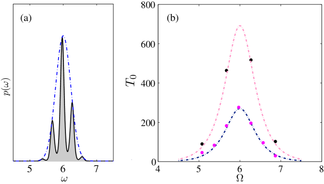
Given the potential model, in the limit of low noise, strong coupling and large delay, the average residence time can be approximated as a function of the common frequency $\Omega$ as follows [188]

$$T_{0}(\Omega)\approx\frac{\pi}{2\lambda}\frac{e^{\frac{\lambda}{D}+\frac{\textbullet\pi^{2}}{8\tau D}}}{\cosh[\frac{\pi(\Omega-\omega_{0})}{2D}]}.$$ (130)

The average residence time increases with the coupling strength $\lambda$ and decreases with the increases in the noise strength $D$. For fixed frequency $\Omega$, effects of the delay on the residence time are limited and the dependency vanishes for long delays. The approximation is validated by numerical results in Fig. 10 (b).

Another interesting related work considers the influence of feedback. With an additional feedback, the system has a stronger symmetry than the one without feedback (120). The corresponding dynamics with feedback is governed by [187]

$$\begin{split}\dot{\theta}_{1}(t)=1+\frac{\lambda}{2}\sin(\theta_{2}(t-\tau)-\theta_{1}(t))+\sin(\theta_{1}(t-\tau)-\theta_{1}(t)),\\ \dot{\theta}_{2}(t)=1+\frac{\lambda}{2}\sin(\theta_{1}(t-\tau)-\theta_{2}(t))+\sin(\theta_{2}(t-\tau)-\theta_{2}(t)).\end{split}$$ (131)

The system also admits in general in-phase and anti-phase solutions. A linear stability analysis for the in-phase solutions leads to the same stability criterion as without feedback. But for the anti-phase solutions, the linear stability analysis becomes complicated. In this case, the only locking frequency is $\Omega=1$ and the anti-phase states lose and regain stability in a Hopf bifurcation [187].

The stability diagram is plotted in Fig. 11. In-phase and antiphase solutions alternate with each other for increasing $\tau$, like in the case without feedback. However, the parameter combinations of the stable in-phase solutions enlarge compared to the case without feedback. Stable antiphase solutions exist for small time delays $\tau$ and small coupling strengths $|\lambda|$. For high $|\lambda|$, oscillatory solutions emerge and coexist with in-phase solutions.

Figure 11: Stable regions in parameter space of $|\lambda|$ and $\tau$ with feedback. In the black regions, in-phase solutions exist and are linearly stable; in the white regions, anti-phase solutions exist and are linearly stable; both states coexist in the gray regions; in the dark gray regions, stable in-phase solutions coexist with oscillatory solutions. Adapted with permission [187]. Copyright 2008, AIP Publishing LLC.

4.1.2 Networks of oscillators with uniform time delay

Next, let us consider networks of oscillators with the same constant time delay for all interactions [183, 189, 193, 194, 195, 191]. Recall that time delays induce various solutions, e.g., bistability between synchronized and incoherent states, unsteady solutions with time-dependent order parameters [183, 187], and multistabilities where synchronized states coexist with stable incoherent states [193].

In terms of the solutions subjected to small perturbations, Yeung and Strogatz [183] provided a detailed analysis on the mean-field Kuramoto model, and derived exact formulas of the stability boundaries of the incoherent and synchronized states for identical oscillators. For bimodal natural frequency distributions, Montbrió et al. [189] found that bimodality induces a quasiperiodic pattern thanks to the existence of a new time scale. Moreover, the stability boundaries of the incoherent state have a completely different structure in the parameter space in contrast to the case with unimodal distribution [183].

To investigate effects of time delays on collective synchronization of coupled oscillators, the self-consistent equations for the order parameter in the stationary state in terms of a Fokker-Planck equation can be derived for a system of globally coupled oscillators with distributed natural frequencies [193]. Due to the time delay, the nonzero synchronization frequency breaks the symmetry of the integration interval of the natural frequency distribution and therein the drifting as well as the synchronous oscillators contribute to the phase coherence. The transition between incoherent states and coherent states is in general discontinuous instead of continuous and the synchronization frequency is suppressed by the time delay. In particular, the synchronization frequency of oscillators in a coherent state is found to decrease with the increases in the time delay. Corresponding curves for the synchronization frequency and phase synchronization with respect to the time delay could also be observed in Rulkov and Hindmarsh-Rose neuron networks with time-delayed chemical synapses [190]. The interplay between the time delay and time-dependent parameters gives rise to low-dimensional echo effects, where time delays strongly affect the magnitude and shape of mean-field oscillations for slow variations of natural frequencies [202]. Additionally, the inclusion of noise to the delayed system induces mode hoppings between coexistent attractors, and the reduction of this system to a nondelayed Langevin equation allows the calculation of analytical solutions of the common frequency distribution and their corresponding residence times [188].

In networks of identical phase oscillators with delayed coupling, one of the simplest model is given by the following equation [184, 195]

$$\dot{\theta}_{i}(t)=\omega_{0}+\frac{\lambda}{k_{i}}\sum^{N}_{j=1}A_{ij}\sin(\theta_{j}(t-\tau)-\theta_{i}(t)),$$ (132)

where each oscillator $i$ receives signals from $k_{i}$ others, $\tau$ is the delay and the adjacency matrix $A_{ij}$ encodes the connection topology of a graph with $A_{ij}=1$ if oscillator $j$ sends signals to oscillator $i$ and $A_{ij}=0$, otherwise. Consider oscillators with uniform in-degree $k$, i.e., $k_{i}=k,\forall i=1,2,\ldots,N$. The synchronized state in which all oscillators move in phase at a fixed common frequency $\Omega$ is given by

$$\theta_{i}(t)=\Omega t,$$ (133)

where $\Omega$ is determined by the following algebraic equation [203, 184]

$$\Omega=\omega_{0}+\lambda\sin(-\Omega\tau),$$ (134)

which is obtained by substituting Eq. (133) into the original dynamics (132). To determine the local stability of the synchronous state (133), consider a linear stability analysis by adding a small perturbation near the synchronous state

$$\theta_{i}(t)=\Omega t+\varepsilon\phi_{i}(t),$$ (135)

where $0<\varepsilon\ll 1$. Providing $\phi_{i}=v_{i}e^{\mu t}$ and substituting Eq. (135) into the original dynamics (132), Earl and Strogatz [184] obtained the first-order approximation of the solution

$$\mathbf{A}v=\sigma^{\rm{A}}v,$$ (136)

with

$$\sigma^{\rm{A}}=\frac{ke^{\mu\tau}\left[\mu+\lambda\cos(\Omega\tau)\right]}{\lambda\cos(\Omega\tau)},$$ (137)

where $\sigma^{\rm{A}}$ is an eigenvalue of $\mathbf{A}$. The synchronized state is linearly stable with $\mathrm{Re}(\sigma^{\rm{A}})<0$ if and only if [183]

$$\lambda\cos(\Omega\tau)>0.$$ (138)

This stability criterion depends on the coupling strength $\lambda$ and on the time delay $\tau$, and it is independent of the network topology. In particular, the criterion of the synchronous state applies to any network in which each oscillator has a uniform in-degree, independent of all other network properties. However, the ability of a network to achieve the full synchronous state also depends on the occurrence and stability of non-synchronous solutions [187]. These states are influenced by the network topology and the delay, and the underlying coupling topology plays an essential role in stability criteria.

To deepen the understanding of effects of time delays on general networks, it is insightful to firstly analyse different types of motifs, e.g., open chains of Kuramoto oscillators, bidirectionally coupled rings, and unidirectionally coupled rings [187]. Depending on networks possessing different symmetries, the delay behaves differently on the bifurcation diagram: (i) in an open chain topology of Kuramoto oscillators, the mathematical analysis is similar to that of two mutually coupled oscillators, i.e., oscillators move either in-phase with each other or anti-phase with their neighbors [187].

(ii) In a unidirectional ring, where oscillator $i$ is coupled to the oscillator $i+1$, the system allows $N$ different frequency-locked solutions. In particular, all oscillators move either in-phase solutions or exhibit spatiotemporal symmetries. Such solutions are stable if and only if $\lambda\cos(\Delta\phi-\Omega\tau)>0$, where $\Delta\phi=\frac{2j\pi}{N}$ with $0\leq j<N$. Moreover, the system also has other unlocked solutions, which could be found numerically. The time delay plays a vital role in inducing multiple solutions without enhancing their linear stability [187]. Under influence of noise, oscillators can switch between different solutions and spend equally much time in different oscillation patterns [188].

(iii) In a bidirectional ring, where each Kuramoto oscillator is coupled to its two neighbors, the stability of $N$ frequency-locked solutions was conducted following the same analysis in unidirectional rings [187]. In particular, two special solutions were addressed where each oscillator moves either in-phase or antiphase with its second nearest neighbor with an even number of oscillators, and the in-phase solutions are stable if and only if $\lambda\cos(\Omega\tau)<0$, whereas solutions with $\Delta\phi=\pm\pi/2$ are always unstable for nonzero delay. As a sufficient stability criterion for other solutions, a state $\theta_{n}(t)=\Omega t+n\Delta\phi$ is stable if $\lambda\cos(\Omega\tau+\Delta\phi)>0$ and $\lambda\cos(\Omega\tau-\Delta\phi)>0$. In contrast to that of the unidirectional ring, the delay of bidirectional ring exhibits different influences on the stability of the in-phase and out-of-phase states [187].

(iv) In this line of research, the relative amount of short cyclic motifs on different classes of networks with the same average degree as the governing topological factor were also considered in networks of identical time-delayed Kuramoto oscillators [192]. The patterns occurring from the cyclic motifs are distinguishable particularly in terms of the momentary frequency dispersion $S^{2}$, which is defined as follows

$$S^{2}\equiv\frac{1}{NT}\int_{0}^{T}\sum\limits_{i}[\dot{\theta}_{i}(t)-\Omega(t)]^{2}dt,$$ (139)

where $\Omega(t)=\sum_{i}\dot{\theta_{i}}(t)/N$ and $T$ denotes a long time intervals. One interesting conclusion is that bidirectional random networks with short cyclic motifs and unidirectional random networks are two opposite ends of a spectrum of different classes of networks [192].

Note that there are two different terms considered: the momentary frequency dispersion $S^{2}$ and the sustained frequency dispersion $\sigma^{2}$ [191]. The sustained frequency dispersion is defined as follows

$$\sigma^{2}\equiv\langle(\Omega_{i}-\Omega)^{2}\rangle,$$ (140)

where $\Omega_{i}=\frac{1}{T}\int^{T}_{0}\dot{\theta}_{i}(t)dt$ and $\Omega$ denotes the average frequency of all oscillators. The two terms exhibit different information. In particular, the momentary frequency dispersion emerges from the cyclic motifs [192]. The pronounced frequency dispersion emerges in networks with binomial degree distribution, along with a relatively smooth transition from synchronization to incoherence with the increases in the time delay $\tau$, in contrast to that of networks with identical degree distributions [191]. Frequency dispersion can also be induced by the time delay in networks with a binomial degree distribution instead of networks with identical degree, i.e. $k_{i}=k$ [191].

Additional to the time delay, it has been shown that phase shifts can show similar features as time delays, e.g., inducing an additional effective phase shift [183, 31]. The interplay between phase shifts and time delays can lead to different oscillator dynamics [195]. This raises the questions of whether time delays and phase shifts play a similar role in networks of coupled Kuramoto oscillators. Consider the following dynamics as a function of a uniform time delay $\tau$ and phase shift $\varphi$ [195]

$$\dot{\theta}_{i}(t)=\omega_{0}+\frac{\lambda}{k_{i}}\sum\limits^{N}_{j=1}A_{ij}\sin(\theta_{j}(t-\tau)-\theta_{i}(t)-\varphi).$$ (141)

The normalization of the coupling strength $k_{i}$ allows in-phase synchronized states with $\theta_{i}(t)=\Omega t$. The collective frequency $\Omega$ therein follows the equation

$$\Omega=\omega_{0}-\lambda\sin(\Omega\tau+\varphi).$$ (142)

To address the effects of the interplay of time delays and phase shifts on synchronization, the collective frequency is kept constant as $\Omega=\Omega_{0}$ by varying $\tau$ and adjusting $\varphi(\tau)$ correspondingly

$$\varphi(\tau)=\Psi-\Omega_{0}\tau,$$ (143)

where $\Psi$ is a constant that determines the value of a constant collective frequency $\Omega_{0}$, and fulfills the following condition

$$\Omega_{0}=\omega_{0}+\lambda\sin(-\Psi).$$ (144)

Although the collective frequency $\Omega$ is kept constant, the relaxation rate $\tau_{r}^{-1}$ (see Sec. 2.3 for definition) does change [195].

To calculate the synchronization rate $\tau_{r}^{-1}$ numerically, initially oscillators are synchronized, and system is then subjected to small random perturbations. When the Kuramoto order parameter approaches $r\sim 1$, relaxation becomes exponential for large times, and $\tau_{r}^{-1}$ is approximated to fit this exponential [195] (see Sec. 2.3). It was observed numerically that the $\tau_{r}^{-1}$ as a function of the time delay $\tau$ displays a characteristic peak with a maximum in globally coupled networks (shown in Fig. 12(a)) and in nearest-neighbor coupled networks [195].

To deepen the insights into the relaxation dynamics as a function of time delays and phase shifts, a linearized method was performed near the synchronized state, $\theta_{i}(t)=\Omega t+\varepsilon\phi_{i}(t)$ with $\varepsilon\ll 1$. The synchronized state is stable if and only if $a>0$, where $a\equiv\lambda\cos(\Psi)$. Substituting this linear approximation into the original system (141) yields the first order in $\phi_{i}$ as

$$\dot{\phi}_{i}(t)=a\sum_{j}b_{ij}[\phi_{j}(t-\tau)-\phi_{i}(t)],$$ (145)

where $b_{ij}\equiv A_{ij}/k_{i}$. Here, only stable states are considered. Via introducing the collective relaxation modes $\eta_{i}(t)=\sum_{j}(d^{-1}_{ij}\phi_{j}(t))$, where $d_{ij}$ follows $\sum_{jk}d^{-1}_{ij}b_{jk}d_{kl}=\mu_{i}\delta_{il}$ and $\mu_{i}$ are eigenvalues of the normalized matrix $b_{ij}$, and given the ansatz $\eta(t)=e^{-\sigma t}$ yield the characteristic equation

$$a-\sigma=a\mu e^{\sigma\tau},$$ (146)

where the index $i$ is dropped for notational simplicity. The solutions follow the Lambert $W$ function, i.e., $W(z)e^{W(z)}=z$ for $z\in\mathbb{C}$. This function has discrete branches $W_{n}(z)$ and each branch corresponds to one relaxation rate $\tau^{-1}_{r_{n}}=\text{Re}(\sigma_{n})$. The slowest relaxation rate $\tau_{r}^{-1}$ is shown as [195]

$$\sigma_{0}=a-\frac{1}{\tau}W_{0}(z_{\tau}),$$ (147)

where $z_{\tau}\equiv\mu a\tau e^{a\tau}$.

Figure 12: Slowest relaxation rate $\tau_{r}^{-1}$ as a function of the coupling delay $\tau$ for a globally coupled system. Numerical simulations of Eqs. 141 and 143 are in circles. Analytical approximation is obtained from Eq. 147. Here, $N=40$, $\omega=1$, $\Psi=5.5$, and $\lambda=0.15$. Adapted with permission from [195].

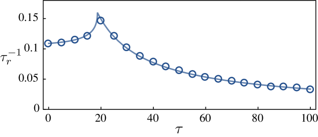
Consider two cases $\mu>0$ and $\mu<0$, which exhibit the Fourier modes in nearest-neighbor coupled oscillators with long wavelengths and short wavelengths, respectively. When $\mu>0$, collective models are the Fourier modes with long wavelengths. In this case, one can show that $\tau_{r}^{-1}$ satisfies [195]

$$\frac{d\tau_{r}^{-1}}{d\tau}=-\frac{\tau_{r}^{-1}}{\tau+(\lambda\cos\Psi-\tau_{r}^{-1})^{-1}}<0,$$ (148)

Note that $\tau_{r}^{-1}$ decreases monotonically, and approaches $0$ for large $\tau$. Moreover, given two eigenvalues if $\mu_{1}>\mu_{2}$, their relative rates obey $\tau_{r1}^{-1}>\tau_{r2}^{-1}$, which is validated numerically.

For $\mu<0$, as suggested by Fig. 12, the relaxation rate displays a peak and its maximum is reached at $\tau^{*}$, where

$$\tau^{*}\equiv\frac{1}{\lambda\cos\Psi}W_{0}\left(\frac{e^{-1}}{|\mu|}\right).$$ (149)

As exhibited numerically, the signs of the derivation of the relaxation rate before and after the threshold are opposite. For $\tau<\tau^{*}$, one can analytically show that $\frac{d\tau^{-1}_{r}}{d\tau}>0$ from Eq. (147). For $\tau>\tau^{*}$, $\frac{d\tau^{-1}_{r}}{d\tau}<0$. The system synchronizes slower as the increases in the time delay. For globally coupled networks, eigenvalues $\mu=(N-1)^{-1}$ and the maximal synchronization rate $\tau^{-1}_{r}$ is located at $\tau^{*}=W_{0}(e^{-1}(N-1))/\lambda\cos\Psi$. In the limit of large time delays, $\tau^{-1}_{r}\approx-\ln(|\mu|)/\tau$, which indicates that the synchronization rates with eigenvalues $\mu$ and $-\mu$ approach the same asymptotic behavior.

4.1.3 Networks of oscillators with distance-dependent time delays

At last of this subsection, we consider an ensemble of coupled Kuramoto oscillators embedded in a metric space and subjected to (distance-dependent) time-delayed interactions [196, 199, 200, 201]. The time delay $\tau_{ij}$ is the time required to transfer a signal from node $j$ to $i$ depending on, for example, the distance between $j$ and $i$ [196]. When oscillators are sparsely and randomly connected, short delays could induce frequency synchronization [196]. Even in a general coupling form, a small fraction of connections with time delays can destabilize synchronous states [197].

Time delays, proportional to the Euclidean distances between interacting oscillators, yield various spatial patterns including traveling rolls, squarelike and rhombuslike patterns, spirals, and targets [199]. Distance-dependent time delays can also induce near regular waves even through oscillators that are randomly coupled [200]. Surprisingly, it is also possible to induce frequency synchronization and allow propagating structures in one-dimensional globally coupled systems [196]. Jeong et al. [199] investigated further effects of the distance-dependent time delay in a two-dimensional array of coupled Kuramoto oscillators, where each oscillator is coupled to oscillators within a finite radius. They found that time delays yield various well defined spatio-temporal patterns, including travelling rolls, squarelike and rhombuslike patterns, spirals, and targets. Moreover, distance-dependent time delays are found to induce traveling waves even with long-range interactions in regular topology [196, 199]. This line of research was also extended to irregular topologies [200]. In the presence of time delays and phase lag, pulse-coupled networks exhibit analogous behaviour, like chimera states [204].

The following system with randomly coupled identical Kuramoto oscillators is generally considered with time delays proportional to Euclidean distances:

$$\dot{\theta}_{i}(t)=\omega_{0}+\frac{\lambda}{k_{i}}\sum\limits_{j}A_{ij}\sin[\theta_{j}(t-\tau_{ij})-\theta_{i}(t)],$$ (150)

where the time delay $\tau_{ij}=\frac{d_{ij}}{v}$. The coupling from oscillators $j$ to $i$ is assumed to be propagated along the distance $d_{ij}$ with finite constant speed $v$. Assume that the oscillators are equally spaced on a ring with circumference $L$ for simplicity and the position $x_{i}$ of the $i$-th oscillator is therein $x_{i}=\frac{L}{N}i$. The distance $d_{ij}$ is taken as the shortest Euclidean distance between oscillators $i$ and $j$, i.e., $d_{ij}=\text{min}\{|x_{j}-x_{i}|,L-|x_{j}-x_{i}|\}$. Note that here identical oscillators are mainly considered. The system of nonidentical oscillators has also attracted much attention [183, 189, 193, 194].

Model (150) with different natural frequencies $\omega_{i}$ can be derived from neural networks to investigate the effect of the large-scale structural connectivity on neural dynamics at the neural population level [205]. The network describes a periodic trajectory (a limit cycle) in phase space and its dynamics can be approximated by the phase $\theta_{i}$ on this limit cycle. $\omega_{i}$ is the intrinsic frequency of node $i$ and is drawn from a fixed Gaussian distribution with mean frequency $\bar{\omega}=60\mathrm{Hz}$ and standard derivation. The coupling term between one node and another is written as a $2\pi$-periodic sin function of their phase difference and is taken into account the interaction delay $\tau_{ij}$. The delay $\tau_{ij}$ from node $j$ to $i$ is calculated using $\tau_{ij}=\left\langle\tau\right\rangle L_{ij}/\left\langle L\right\rangle$, where $\left\langle\tau\right\rangle$ denotes the mean delay, $L$ is the fiber length matrix and $\left\langle L\right\rangle$ is the mean fiber length. The biologically-based Kuramoto model in the presence of time-delayed interactions gives rise to the emergence of slow neural activity fluctuations with their patterns significantly correlated with the empirically measured functional connectivity (see also Sec. 9.2 for more applications of neuronal models).

Noteworthy, assuming a fixed amplitude and taking only the phase dynamics into account, the dynamics of the full Stuart-Landau equation with feedback can be reduced to a delay-coupled Kuramoto model [206] and its linear stability analysis can also be derived via a similar mathematical process [184, 187].

Wave formation is observed in randomly coupled oscillators [200], where, for each oscillator $i$, $\langle k\rangle/2$ oscillators are randomly chosen to couple to $i$ bidirectionally. Moreover, the system shows different behaviors, including wave states and in-phase state, in terms of different topologies as shown in Fig. 13 with the difference of panels from (a) to (e) in the coupling topology and the initial phase configurations. To quantify the oscillating behaviors, the average frequency $\Omega=\frac{1}{N}\sum_{i}\dot{\theta}_{i}$ and the frequency dispersion $\sigma=\sqrt{\frac{1}{N}\sum_{i}(\dot{\theta}_{i}-\Omega)}$ are defined. With the increases of the average degree $\langle k\rangle$ (as shown from Fig. 13(a) to (c)), the system exhibits wave states similar to that of all-to-all coupling case (Fig. 13(d)). Additionally to the wave states in Fig. 13(c), the system can also exhibit near in-phase synchronous states in Fig. 13(e).

Figure 13: Phase of the oscillators with $\omega_{0}=\pi/10$,$N=400$, $K=0.4$, $1/v=0.22$, and $L=400$. (a) The average degree $\langle k\rangle=4$, the average frequency $\Omega\approx 0.31$, and the frequency dispersion $\sigma\approx 0.05$. (b) $\langle k\rangle=8$: a wave state with winding number $n=4$, $\Omega\approx 0.295$, and $\sigma\approx 0.015$. (c) $\langle k\rangle=20$: a wave state with $m=4$, $\Omega\approx 0.2933$ and $\sigma=4\times 10^{-4}$. (d) All-to-all coupling: a wave state with $m=4$, $\Omega=0.291$, and $\sigma=10^{-5}$. (e) $\langle k\rangle=20$: a near in-phase synchronous state, $\Omega=0.0424$, and $\sigma<10^{-5}$. Reprinted with permission from [200]. Copyright 2011 by the American Physical Society.

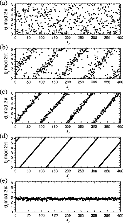
In the case when phase differences remain typically small in the system, Eguiluz et al. [201] considered a linearization of a set of coupled Kuramoto oscillators. In this case, the corresponding governing dynamics becomes

$$\dot{\theta}_{i}(t)=\omega_{i}+\lambda\sum^{N}_{j=1}A_{ij}\left[\theta_{j}(t-\tau_{ij})-\theta_{i}(t)\right].$$ (151)

All oscillators rotate at constant speed $\Omega$ with sufficiently small phase differences and their phases are represented by

$$\theta_{i}(t)=\Omega t+\phi_{i},$$ (152)

where $\phi_{i}$ is the initial phase of the $i$-th oscillator. The dependence of the locking frequency $\Omega$ on the network parameters and on the time delays is given by [201]

$$\Omega=\frac{\left\langle\bm{\omega}\right\rangle}{1+\left\langle\mathbf{T}\right\rangle},$$ (153)

and the phases

$$\frac{\omega_{i}-\left\langle\bm{\omega}\right\rangle-(\omega_{i}\left\langle\mathbf{T}\right\rangle-\left\langle\bm{\omega}\right\rangle T_{i})}{1+\left\langle\mathbf{T}\right\rangle}=(\mathbf{L}\bm{\phi})_{i},$$ (154)

where $\boldsymbol{\omega}$ is the frequency vector with components $\omega_{i}$, $\mathbf{T}$ is a vector of components $T_{i}=\sum_{j}A_{ij}\tau_{ij}$ indicating the total delay on node $i$, $\mathbf{L}$ is the Laplacian matrix with $L_{ij}=k_{i}^{\mathrm{in}}\delta_{ij}-A_{ij}$, $k_{i}^{\mathrm{in}}$ is the in degree of the node $i$, $\delta_{ij}$ is the Kronecker delta, $\boldsymbol{\phi}$ is the phase vector with components $\phi_{i}$, $\left\langle\boldsymbol{x}\right\rangle=\sum_{i}c_{i}x_{i}$ and $\bm{x}$ is normalized with $\sum_{i}c_{i}=1$, with $c_{i}$ being the components of the left eigenvector of $\mathbf{L}$ with eigenvalue 0. Without loss of generality, the coupling strength is recalled, i.e. $\lambda=1$. If all nodes of the network are reached by at least one node, Eq. 151 has a unique phase locked solution given by Eqs. (153) and (154) [201].

For uncorrelated and undirected networks of identical oscillators with constant time delay, i.e. $\omega_{i}=\omega_{0}$ and $\tau_{ij}=\tau$, the analytic formulas of the mean phases $\Phi_{k}$ of nodes with degree $k$ and the locking frequency $\Omega$ are obtained as [201]

$$\Phi_{{k}}=\frac{\Omega\left\langle k\right\rangle\tau}{k}+a,$$ (155)

and

$$\Omega=\frac{\omega_{0}}{1+\left\langle k\right\rangle\tau},$$ (156)

where $a$ is an arbitrary constant. This indicates that in uncorrelated networks the phase difference of nodes depends on their degree difference. In this limit, the locking frequency depends on the average degree but is independent of the degree distribution.

Along the lines of these topics, considering the limit of $N\rightarrow\infty$, Ko and Ermentrout [197] analyzed effects of axonal time delay on synchronization and wave formation using an approximate equation, which for discrete oscillators is equivalent to an equation for a continuum of oscillators as follows

$$\frac{\partial\theta(x,t)}{\partial t}=\omega_{0}+\frac{\lambda}{\overline{P}}\int^{L/2}_{-L/2}P(x,x+y)\sin(\theta(x+y,t)-\theta(x,t)-2\pi\tau|y|)dy,$$ (157)

where $\tau$ is the relative unit time delay, $P(x,x+y)$ is the connecting probability between oscillators at $x$ and $x+y$, oscillators are located uniformly along a ring with circumference $L$, $x_{i}=Li/N$, and $\overline{P}$ is the average connecting probability defined by $\overline{P}=\int^{L/2}_{-L/2}\int^{L/2}_{-L/2}P(x,y)dydx$. To simplify the notation, without loss of generality, $L$ is set unity, i.e., $L=1$. For randomly coupled oscillators with perfect synchronous solutions or traveling wave solutions, $P(x,x+y)$ is a constant. Therefore, the continuum equation can be simplified and is exactly the form as that of globally coupled case as follows

$$\frac{\partial\theta(x,t)}{\partial t}=\omega_{0}+\lambda\int^{1/2}_{-1/2}\sin(\theta(x+y,t)-\theta(x,t)-2\pi\tau|y|)dy.$$ (158)

Providing that the possible solutions obey the following form $\theta(x,t)=\Omega_{q}t+qx$, where $\Omega_{q}$ is the synchronization frequency, $q=2m\pi$ is the wave vector and $m=0,\pm 1,\pm 2,\ldots$. Substituting these solutions into Eq. 158 yields

$$\Omega_{q}=\omega_{0}+\lambda\left\{\int^{1/2}_{0}\sin(qy-2\pi\tau y)dy+\int^{0}_{-1/2}\sin(qy+2\pi\tau y)dy\right\}.$$ (159)

. In Figure 14(a), the synchronization frequency $\Omega$ as a function of the relative unit time delay $\tau$ and winding number $m$ is obtained from Eq. 159. Symbols and error bars are obtained numerically considering randomly coupled oscillators. Numerical and theoretical results fit well to each other. Thick parts of the curves are identified by the linear stability analysis. Dashed vertical lines indicate the minimum of the maximal real values of eigenvalues and correspond to the most locally stable states. The frequency dispersions are small around the dashed vertical lines and enlarge when states move away from these lines. Order parameter also reflects this trend [197].

Consider the stability of this possible solutions and let $\theta(x,t)=\Omega_{q}t+qx+\varepsilon\phi(x,t)$, where $\varepsilon\ll 1$ and $\phi(x,t)=e^{iax}e^{\sigma_{a}t}$ with $a$ following the form $2\pi q$ and $q=0,\pm 1,\pm 2,\ldots$. Via inserting these quantities into Eq. 158, the real part of $\sigma_{a}$ follows

$$\text{Re}(\sigma_{a})=\lambda\int^{1/2}_{-1/2}\cos(qy-2\pi\tau|y|)[\cos(ay)-1]dy.$$ (160)

As shown in Fig. 14(b), maximal values of $\text{Re}(\lambda_{a})_{\text{max}}$ as a function of $\tau$ are shown and their negative values correspond to the stability region as thick curves. Bifurcations occur at the end points of the thick curves. The results are even good for very sparsely coupled cases with $k_{i}\ll N$.

Figure 14: States and their linear stability as a function of the relative unit time delay $\tau$ with $\omega_{0}=\pi/2$ and $\lambda=1$. Thick curves indicate stable states identified by the linear stability analysis of the system (158). (a) Synchronization frequency $\Omega$. Symbols and error bars denote the time average of $\Omega$ and the frequency dispersion calculated numerically with $N=1600$ and $\langle k\rangle=40$. Dashed vertical lines are located at the minimum of $\text{Re}(\sigma_{a})_{\text{max}}$. (b) The maximum real part $\text{Re}(\sigma_{a})_{\text{max}}$ of eigenvalue $\sigma_{a}$ given by Eq. 160. Adapted with permission from [197]. Copyrighted by the American Physical Society.

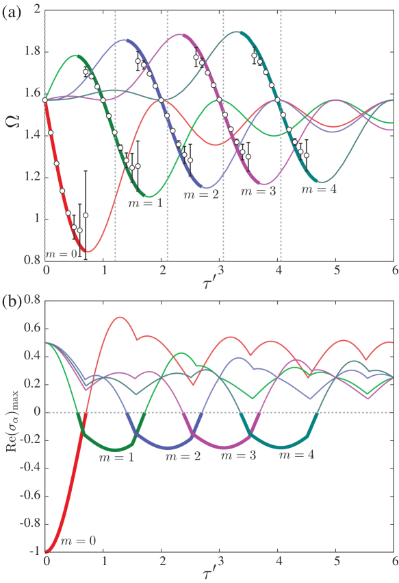
Additionally to the distance-dependent time delays, time delay $\tau$ could vary according to a distribution [196, 197, 198, 201, 200, 207]. In the continuum limit, where $N\rightarrow\infty$, Lee et al. [198] provided a framework for the study of delay heterogeneity on the stability of incoherent states and the dynamics transitions from stable incoherent states to stable coherent states, using the OA ansatz [32]. In comparison to the case with uniform time delay, spread in the delay distribution function greatly affects the system dynamics, e.g., the critical coupling.

It is worth noting that the influence of time delays was also investigated under the presence of time-varying parameters [202], a model that is relevant for the study of effects of anaesthesia on macroscopic dynamics of the brain [208]. Specifically, instead of solely having time-dependent coupling function, natural frequencies and coupling strength are also allowed to vary over time [202]. The problem was tackled using the OA ansatz [32, 202] .

4.2 Time-varying coupling

Due to the ubiquity of synchronization in complex systems, it is interesting to understand effects of time-varying interactions on collective behaviors of networked oscillators. Adaptive mechanisms can be found in biological systems [209] and neural systems [210], e.g., the synchronization of pacemaker cells in the heart, evolving patterns of neuronal synchronization in the brain [211], and a typical Asian firefly specie, Pteroptyx malaccae, with adaptive frequency to achieve perfect synchronization with stimulating frequency [209] (see Sec. 7).

Feedback theory is commonly used for time-varying coupling, and it is one of the most important ideas developed in the last century, with fundamental implications especially for biological neural systems [210]. For example in neuroscience, spike-timing dependent plasticity (STDP) enhances synchronization of neural activity via enlarging the synchronization zones, decreasing the relaxation time, and increasing its robustness against perturbations [212, 213]. In networked Kuramoto oscillators, STDP can give rise to multistability [214].

Adaptive scheme can suppress the negative effect of the heterogeneity in oscillator networks [215, 216, 217, 218]. Even in a system of identical Kuramoto oscillators, the presence of coupling plasticity induces the occurrence of multi-stable states, i.e., the existence of a desynchronized state and a state consisting of two anti-phase clusters [219]. In adaptive and multilayer networks in the absence of frequency-degree corrections, explosive synchronization occurs [181] (see Sec. 5). Additional to adaptive weights (coupling), adaptive natural frequency induces special features, including long waiting times before synchronization and three stability regimes [211, 220].

Here we aim at presenting recent results of synchronization on networks of Kuramoto oscillators, where coupling strengths slowly adapt. We will also discuss effects of different kinds of adaptive coupling schemes on global and local synchronization.

The system consists of an ensemble of $N$ phase oscillators and its governing dynamics is given by

$$\dot{\theta}_{i}=\omega_{i}+\lambda\sum_{j\in\mathcal{N}_{i}}w_{ij}(t)\sin(\theta_{j}-\theta_{i}),$$ (161)

where each oscillator $i$ has the randomly assigned natural frequency $\omega_{i}$ and interacts with $K$ randomly selected oscillators, which form the set $\mathcal{N}_{i}$. Coupling $w_{ij}$ is the non-negative and time-dependent weight of a directed link from node $j$ to $i$ in  [221, 222]. The adaptive evolution of the weights $w_{ij}$ is defined as follows [221]

$$\dot{w}_{ij}(t)=p_{ij}-\left(\sum_{l\in\mathcal{N}_{i}}p_{il}\right)w_{ij}(t),$$ (162)

where $p_{ij}$ quantifies the local synchronization between nodes $i$ and $j$ over a characteristic memory time $T$, and it is governed by

$$p_{ij}=\frac{1}{T}\left|\int^{t}_{-\infty}e^{-(t-t^{\prime})/T}e^{i[\theta_{i}(t^{\prime})-\theta_{j}(t^{\prime})]}dt^{\prime}\right|.$$ (163)

The sum of the incoming weights of each nodes is kept constant at all times, i.e., $\sum_{j\in\mathcal{N}_{i}}w_{ij}=1$. In directed networks with the same incoming and outgoing links, the coupling weights $w_{ij}$ can also bes adjusted as [222]

$$\dot{w}_{ij}(t)=w_{ij}(t)\left[s_{i}p_{ij}-\sum_{j}w_{ij}(t)p_{ij}\right],$$ (164)

where $s_{i}$ denotes the sum of the total incoming strength, i.e., $s_{i}=\sum^{N}_{j=1}w_{ij}$, and $p_{ij}$ denotes the average phase correlation between nodes $i$ and $j$ over the time interval $[t-T,t]$ as

$$p_{ij}=\frac{1}{T}\left|\int^{t}_{t-T}e^{i[\theta_{j}(t^{\prime})-\theta_{i}(t^{\prime})]}dt^{\prime}\right|.$$ (165)

Note that here memory dependent adaptation mechanisms are considered. The local phase correlation $p_{ij}$ could also be instantaneous  [223].

The adaptive scheme has the form of the replicator equation and exhibits the feature of homophily and homeostasis, accounted for by, respectively, the first and the second term in the right-hand side of Eq. 162 and 164. When the first term is larger than the second one, the adaptive mechanism will enhance their coupling strength, which exhibits effects of homophily. On the other hand, the mechanism will depress their coupling strength, as effects of homoeostasis [223].

The influence of adaptive coupling on global synchronization $r$ and local synchronization $r_{\text{link}}$ between connected links is investigated with the respective definitions [221]

$$r=\lim_{\Delta t\rightarrow\infty}\frac{1}{\Delta tN}\int^{t_{s}+\Delta t}_{t_{s}}\left|\sum^{N}_{j=1}e^{i\theta_{j}(t^{\prime})}\right|dt^{\prime},$$ (166)

and

$$r_{\text{link}}=\frac{1}{N}\sum^{N}_{i=1}\sum^{N}_{j\in\mathcal{N}_{i}}w_{ij}\lim_{\Delta t\rightarrow\infty}\frac{1}{\Delta t}\left|\int^{t_{s}+\Delta t}_{t_{s}}e^{i[\theta_{j}(t^{\prime})-\theta_{i}(t^{\prime})]}dt^{\prime}\right|,$$ (167)

where $t_{s}$ identifies the beginning of averaging the global and local synchronization over a suitably long time interval denoted by $\Delta t$. Intuitively, $r$ quantifies the global time averaged order parameter and $r_{\text{link}}$ the time averaged local synchronization between connected nodes. The two measures coincide with each other for very small or very high coupling strengths but become different with the emergence of modularity, where $r_{\text{link}}>r$ and only local synchrony occurs.

Figure 15: Projection of (a) global synchronization $r$ and (b) local synchronization $r_{\text{link}}$ over the parameter space of $(T,\lambda)$ in a directed weight-adapted network. (c) Time evolution of global order parameter $r(t)$ considering $T=15$ for different couplings. Remaining parameters: $t_{s}=2000$, $\Delta t=1000$ and $T=15$. From [221].

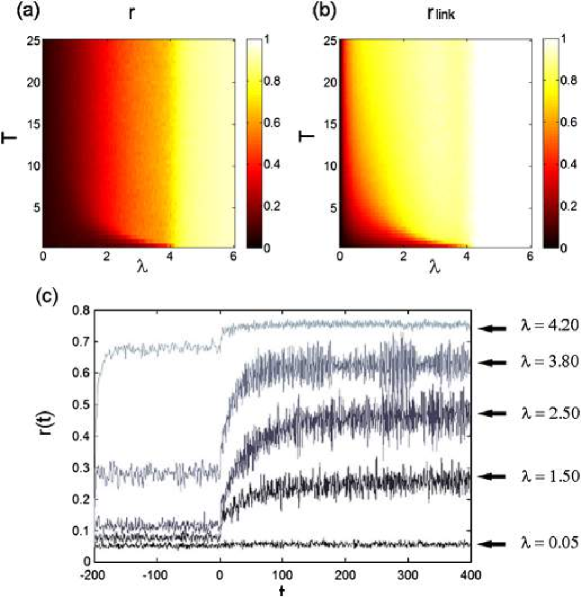
(i) Let us consider first the adaptive coupling in Eq. 162. In simulations, the system is integrated with initial values $w_{ij}=1/K$ and without the adaptive coupling during the first $200$ time units. Subsequently, at the time instant defined as $t=0$, the adaptation mechanism (162) is switched on. After $t_{s}$ integrating time units, $r$ and $r_{\rm{link}}$ are monitored over another $\Delta t$ time periods. The time evolution of the instantaneous order parameter $r(t)$ is shown in Fig. 15 (c) via varying the value of $\lambda$ and fixing $T=15$, showing the striking result that the adaptive mechanism generally enhances global synchronization $r(t)$ for $t>0$ in comparison to that for $t<0$. This result was also observed with different adaptive mechanisms [224].

Figure 15 plots the global synchronization $r$ in (a) and the local synchornization $r_{\text{link}}$ (b) with respect to $\lambda$ and $T$. For large values of $T$, $r$ and $r_{\text{link}}$ solely depend on the coupling $\lambda$ up to the threshold $\lambda_{c}$, which is determined as in the classical Kuramoto model [40], i.e., $\lambda_{c}^{\rm{KM}}=\frac{2}{\pi g(0)}$ (Eq. 9). Within this period, due to the emergence of modular structure, $r_{\text{link}}$ grows much faster than $r$, persisting as such for a wide region in the plane (for $\lambda<1$ and $T>1$). With increasing $\lambda$ beyond $\lambda_{c}$, higher global and local synchronizations are achieved. In this case, $p_{ij}\approx 1$ and $w_{ij}\approx 1/K$ (one can also approximate its value by setting $\dot{w}_{ij}=0$ in Eq. 162).

To deepen the understanding of this structure, the modularity of the partition of networks is measured by its modular cohesion $MC$ as follows [221]

$$MC=\frac{1}{N}\sum^{M}_{\mu=1}\sum_{i,j\in C_{\mu}}w_{ij},$$ (168)

where the fast community detection algorithm [225, 226] allows us to split the network into $M$ non-overlapping communities and $C_{\mu}$ stands for the $\mu$th community. $MC$ quantifies the degree of the partition, takes values within $[0,1]$, and $MC=1$, when the network is split into disconnect modules. Interestingly, the network is separated into components when $\lambda$ is relatively low and $T$ is relatively high (Fig. 16). At small values of $\lambda$, the adaption mechanism redistributes the weights, which leads to a highly heterogeneous topology. With the increases of $\lambda$, more and more distinct modules occur and $MC$ increases respectively. When $\lambda>\lambda_{c}$, the coupling weights are persistent at a constant value $1/K=0.05$ (the initial value) and all oscillators belong to a single synchronous component. In this case, the adaptation mechanism is negligible.

Figure 16: Modularity cohesion $MC$ (Eq. 168) as a function coupling $\lambda$ and characteristic memory time $T$ for networks consisting of $N=300$ oscillators. From [221].

(ii) Secondly, we consider directed networks with the same governing dynamics (161) but different adaptive-coupling schemes (164). Following the same simulation process, the time evolution of $r$ can exhibit quasi-periodic oscillations for some special coupling strengths [222]. Interestingly, the network dynamics with competitive interactions (Eqs. 161, 164 and 165) presented similar behaviors as in the above analysis of Fig. 15. Specifically, the projections of $r$ and $r_{\rm{link}}$ on the plane $(\lambda,T)$ also exhibit the presence of incoherent, partially ordered and totally synchronized regimes. In the incoherent state, a modular structure emerges, and a large internal synchronization of each modular is achieved but without global and local synchronization. At low coupling strength, a distribution of weights can be fitted by a power-law distribution. With increasing $\lambda$, the system comes to the partially ordered phase, where $r$ oscillates. Meanwhile, multiple components coexist and within each component perfect local synchronization is achieved. For high $\lambda$, the network dynamics ends up in a fully synchronized state and the stationary network with $\dot{w}_{ij}=0$ in (164) is very similar to the initial regular network without adaptation, where each link shares the same weights, i.e., $w_{ij}=1/K$.

The above results are induced by the competitive mechanisms (162) and (163) or (164) and (165). Other adaptive mechanisms proportional to the instantaneous phase difference between the oscillators have also been considered [224, 216, 227]. For instance, Aoki and Aoyagi [228] investigated coevolving dynamics in a weighted network of identical oscillators as follows

$$\dot{\theta}_{i}=\omega_{i}-\frac{1}{N}\sum_{j}w_{ij}\sin(\theta_{i}-\theta_{j}+\varphi),$$ (169)

where the natural frequency is identical with $\omega_{i}=\omega_{0}=1$, without loss of generality. The constant phase shift denoted by $\varphi$ is induced by a short delay of the coupling and the coupling weight from the $j$th to the $i$th oscillator is denoted by $w_{ij}$. The dynamical model for the coupling weights $w_{ij}$ depends on the relative timing of phase difference as follows

$$\dot{w}_{ij}=-\varepsilon\sin(\theta_{i}-\theta_{j}+b),$$ (170)

where $\varepsilon$ determines the time scale of the evolution of the coupling weights with $\varepsilon\ll 1$ and $b$ a different phase shift. The coupling $w_{ij}$ is bounded within the range of $[-1,1]$, and outside the boundary, $w_{ij}$ is immediately set to the approximate bounded value ($1$ or $-1$). An alternative method can be implemented by including a nonlinear term similar as in [224] and the results are qualitatively the same (see Fig. 17). With this coevolving dynamical coupling, the system has three distinct types of self-organized phase patterns (Fig. 17 (b)): a two-cluster state, a coherent state, and a chaotic state, depending on $\varphi$ and $b$. The results are independent of the network parameter values, and are robust against the topological differences between the SF and the all-to-all connections.

A generalization of the order parameter (Eq. 2) can be defined as

$$R_{m}=\left|\frac{1}{N}\sum^{N}_{j=1}e^{im\theta_{j}}\right|,$$ (171)

where $m=1$ or $2$. $|R_{1}|$ quantifies the degree of asymmetry in clustering (refer to other sections), while $|R_{2}|$ quantifies the degree of cluster synchrony in the system [229] and converges to $1$ when a two-cluster state with anti-phase synchronization emerges.

The normalized rate of change of the weights averaged over all connections is given by [230]

$$\Delta K(t)=\frac{1}{N(N-1)}\sum_{i\neq j}\frac{|w_{ij}(t)-w_{ij}(t-\delta)|}{\delta},$$ (172)

where $\delta$ is a sampling interval $\delta\approx\frac{2\pi}{\omega_{0}}\ll 1/\varepsilon$. In the region $b\in[-\pi,0]$, the time evolution of coupling weights exhibits the Hebbian-like characteric and this is a positive feedback.

In the two-cluster state in Fig. 17 (b) and (c-d), $R_{1}$ is kept close to zero, $R_{2}$ converges to $1$ with anti-phase synchronization. The rate $\Delta K(t)$ becomes zero if the coupling weights are in frozen states, where oscillators within the same cluster run at the same frequency. The ratio of the populations in the two clusters depends on the initial conditions. On the other hand, in the coherent state in Fig. 17 (b) and (e-f), the system is in the steady state and the rate of change of weights $\Delta K$ remains close to zero. To characterize it, the autocorrelation function $C(\tau)=\left\langle|\frac{1}{N}\sum_{j}e^{i\theta_{j}(t)}e^{-i\theta_{j}(t-\tau)}|\right\rangle$ is defined showing that $C(\tau)$ remains close to $1$, i.e., the oscillators are in the steady state. In right parameter region of Fig. 17 (b), where both the two-cluster state and the coherent state become unstable in Fig. 17 (g-h), the system behaves chaotically with positive Lyapunov exponents and the number of positive Lyapunov exponents is a linear function of the number of degrees of freedom of the system. Furthermore, $\Delta K$ does not decay and $C(\tau)$ converges to zero. Additional to the two-cluster state, the system can be designed to exhibit an $m$-cluster state by choosing an appropriate coupling evolution function, e.g. $\dot{w}_{ij}=\cos[(m-1)\theta]$ [230].

Figure 17: Coevolving dynamics on a scale-free network and its topology is shown in (a). Three regimes are exhibited in (b) as a function of the characteristic $b$ in terms of the second order parameter $\overline{R}_{2}$, the long-time correlation $\overline{C}$ and the rate of change of weights $\overline{\Delta K}$ with $a=0.3\pi$ and $\varepsilon=0.005$. Time evolution of phase and phase vs degree are shown in (c-d) for the two-cluster state with $b=-0.7\pi$, (e-f) for the coherent state with $b=-0.1\pi$, and (g-h) the chaotic state with $b=0.7\pi$. Adapted with permission from [230]. Copyrighted by the American Physical Society.

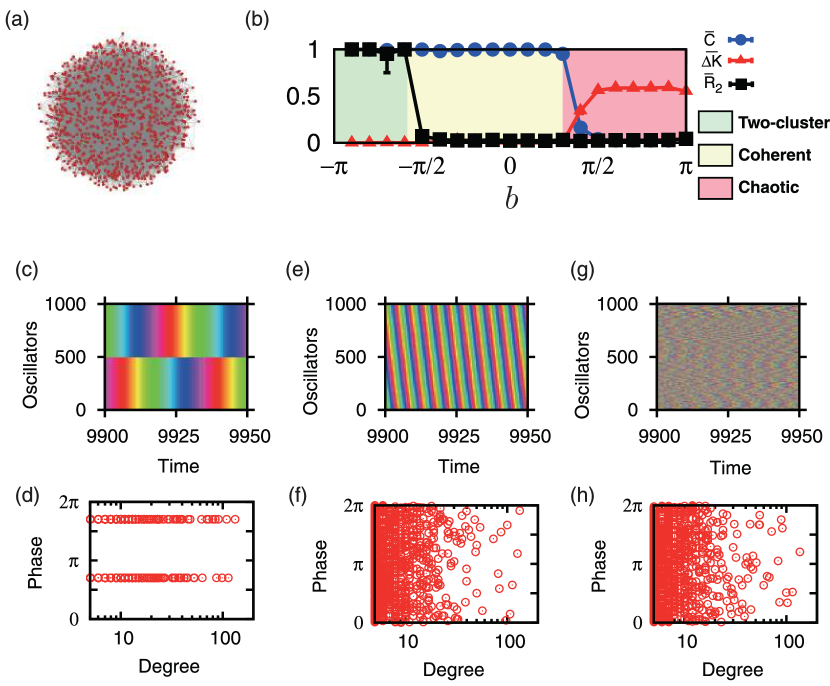
5 Correlations between dynamics and topology (Explosive synchronization)

Several works have verified the occurrence of discontinuous synchronization transitions in the tradition Kuramoto model since 90’s [231]. Regarding the model without inertia, in 1992, Bonilla et al. [231] provided one of the first studies on first-order transitions in complete graphs. The authors further showed that such transitions could emerge when bimodal frequency distributions are considered. After this work, only in 2005 the subject of abrupt transitions in the first-order Kuramoto model was brought to attention again [56]. Analyzing the model with uniform frequency distributions, Pazó [56] showed that suddenly after a given critical coupling $\lambda_{c}$, all the population of oscillators is entrained in the mean-field, making the order parameter $r$ to “jump” from $r\sim 0$ to $r_{c}\lesssim 1$ with the dependence $r-r_{c}\propto(\lambda-\lambda_{c})^{2/3}$, for $\lambda>\lambda_{c}$. The work by Pazó triggered further investigations devoted to the analysis of first-order transitions [232, 233, 234]. In particular, Basnarkov and Urumov [232] analyzed the phase transition in the Kuramoto model and also generalized the results to unimodal frequency distributions composed by a plateau followed by tails in the form $|\omega-\omega_{0}|^{m}$. They observed discontinuous transitions for $m>0$. The same authors later reported that asymmetric frequency distributions could also lead to this dependency of the order parameter as a function of coupling [233].

Further works verified that the same conditions to yield discontinuous transitions in fully connected graph do not necessarily have the same effect in heterogeneous topologies [29, 14]. However, in 2011 Gómez-Gardeñez et al. [30] firstly demonstrated the occurrence of a discontinuous transition – or “explosive synchronization” (ES) as named by them – in SF networks. The authors suggested that the correlation between topology and dynamics is the mechanism responsible for such a transition. More specifically, they considered the natural frequencies to be positively correlated with the degrees in the form $\omega_{i}=k_{i}$, where $k_{i}=\sum_{j=1}^{N}A_{ij}$ is the degree of node $i$. By using a random network model [235] able to tune continuously from ER to BA networks via controlling a single parameter $\alpha\in[0,1]$ in the model, the authors showed that explosive synchronization only happens for $\alpha=0$, i.e., when the network is SF with a degree distribution given by $P(k)\sim k^{-\gamma}$, as shown in Fig. 18 [30]. Furthermore, to analyze the network dynamics locally, the authors also considered the effective frequency

$$\omega_{i}^{\rm{eff}}=\frac{1}{T}\int_{t}^{t+T}\dot{\theta}_{i}(\tau)d\tau.$$ (173)

Figure 19 shows the corresponding dependency of $\omega_{i}^{\textrm{eff}}$ for the forward propagation of coupling $\lambda$ along with the effective frequency for each group of nodes with degree $k$, $\left\langle\omega\right\rangle_{k}=\sum_{[i|k_{i}=k]}\omega_{i}^{\rm{eff}}/(NP(k))$ [30]. As we can see, for Fig. 19(a)-(c) the groups of nodes join smoothly the synchronous component as the coupling is increased. However, for $\alpha=0$ (Fig. 19(d)) all nodes join the giant synchronous component abruptly at $\lambda_{c}\approx 1.4$, evolving with $\left\langle\omega\right\rangle_{k}=\left\langle k\right\rangle=6$ [30].

Figure 18: Synchronization diagram $r(\lambda)$ for networks generated from the model proposed in [235] for (a) $\alpha=1$ (ER), (b) $\alpha=0.6$, (c) $\alpha=0.2$ and (d) $\alpha=0$ (BA). All networks have $N=10^{3}$ and $\left\langle k\right\rangle=6$. Reprinted with permission from [30]. Copyright 2011 by the American Physical Society.

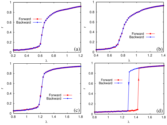
These findings led the authors to conjecture that the necessary condition for the emergence of an abrupt variation in the order parameter is the correlation between the dynamics and the network structure. Other dynamical processes in networks share similar characteristics, such as the case of percolation and epidemic spreading, where there is also a microscopic mechanism that leads to the abrupt transition [236, 237, 238, 239, 240].

Figure 19: Effective frequencies $\left\langle\omega\right\rangle_{k}$ as a function of coupling $\lambda$ for networks using model [241] with (a) $\alpha=1$ (ER), (b) $\alpha=0.6$, (c) $\alpha=0.2$ and (d) $\alpha=0$ (BA). All networks have $N=10^{3}$ and $\left\langle k\right\rangle=6$. Reprinted with permission [30]. Copyright 2011 by the American Physical Society.

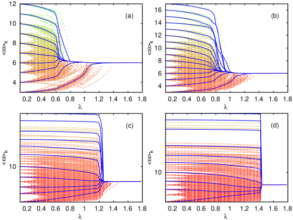
5.1 Analytical approaches

The first work on explosive synchronization focused mostly on the numerical analysis of the model in complex networks and the theoretical calculation of the critical coupling for a star graph. Naturally the discovery of such transitions raised many questions on the subject, a fact that motivated many following works [30, 242, 243, 244, 245, 246, 247, 248, 249, 138, 139, 140, 250, 251, 252, 143, 141, 253, 254, 255]. The first analytical approach to the model in networks without degree-degree correlations was carried out by Peron and Rodrigues [242]. More specifically, the authors considered the equations of motion (Eq. 42) in the continuum limit for the case in which $\omega=k$, i.e.,

$$\dot{\theta}=k+\lambda k\int dk^{\prime}\int d\theta^{\prime}\frac{k^{\prime}P(k^{\prime})}{\left\langle k\right\rangle}\rho(\theta^{\prime},t|k^{\prime})\sin(\theta^{\prime}-\theta),$$ (174)

where $\rho(\theta,t|k)$ is the density of oscillators with phase $\theta$ at time $t$ for a given degree $k$, similarly as before. Using the corresponding definition for the order parameter $r$ in the continuum limit

$$re^{i\psi(t)}=\frac{1}{\left\langle k\right\rangle}\int dk\int d\theta kP(k)\rho(\theta,t|k)e^{i\theta}$$ (175)

and rewriting the equations in the rotating frame it is possible to show that the real part of the order parameter is given by [242]

$$\left\langle k\right\rangle r=\int_{\left\langle k\right\rangle/(1+\lambda r)}^{\left\langle k\right\rangle/(1-\lambda r)}dkP(k)k\sqrt{1-\frac{1}{\lambda^{2}r^{2}}\left(\frac{k-\left\langle k\right\rangle}{k}\right)^{2}}.$$ (176)

Changing the variable in Eq. 176 and letting $r\rightarrow 0^{+}$ we obtain [242]

$$\lambda_{c}=\frac{2}{\pi\left\langle k\right\rangle P(\left\langle k\right\rangle)},$$ (177)

which is the critical coupling for the onset of synchronization. It is interesting to note that for the case in which natural frequencies are equal to degrees, the critical coupling no longer depends on the ratio between the first moments of the degree distribution $\left\langle k\right\rangle/\left\langle k^{2}\right\rangle$, in contrast to the case where the frequencies are drawn from a unimodal and even distribution [60]. Noteworthy, strictly speaking, the result in Eq. 177 is valid for networks with symmetric $P(k)$, although it provides good estimates for $\lambda_{c}$ in SF networks with reasonable size [242]. Following a similar analysis, the expression for $\lambda_{c}$ was recently generalized for networks with $P(k)\sim k^{-\gamma}$ and it is given by [256]

$$\lambda_{c}=\frac{2\frac{(\gamma-1)^{\gamma-2}}{(\gamma-2)^{\gamma-1}}}{\sqrt{\pi^{2}+\left[\log(\gamma-2)-\sum_{i=1}^{\gamma-3}\frac{1}{i}\left(\frac{\gamma-1}{\gamma-2}\right)^{i}\right]^{2}}},$$ (178)

which is valid for any integer $\gamma>2$.

Figure 20: (a) Example of solution of Eq. 184 for an ER network with $\left\langle k\right\rangle=10$. The dashed lines correspond to the curves $x/\lambda$, whose intersection with $\mathcal{R}(x)$ yield the solutions of Eq. 183 leading to (b) the order parameter $r$ as a function of $\lambda$. Adapted with permission from [249]. Copyrighted by the American Physical Society.

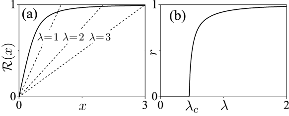
A different analysis of explosive synchronization was carried out by Coutinho et al. [249], where further properties of the model were uncovered. Noting that in the rotating frame the equations of motion are written as $\dot{\theta}_{i}-\Omega=(k_{i}-\Omega)+\lambda rk_{i}\sin(\psi-\theta_{i})$, with $\Omega$ being the average frequency, it is possible to rewrite the order parameter as

$$re^{i\psi(t)}=\frac{1}{N\left\langle k\right\rangle}\sum_{\left|k_{j}-\Omega\right|\leq k_{j}\lambda r}k_{j}e^{i\theta_{j}}+\frac{1}{N\left\langle k\right\rangle}\sum_{\left|k_{j}-\Omega\right|>k_{j}\lambda r}k_{j}e^{i\theta_{j}},$$ (179)

where the first and second terms are the contributions due to locked and drifting oscillators, respectively. Taking the continuum limit of Eq. 179 we can write each contribution as

$$r_{{\rm{lock}}}=\frac{1}{\left\langle k\right\rangle}\int_{|k-\Omega|\leq\lambda kr}dkP(k)k\sqrt{1-\left(\frac{k-\Omega}{\lambda kr}\right)^{2}}$$ (180)

and

$$r_{{\rm{drift}}}=\frac{1}{\left\langle k\right\rangle}\int_{|k-\Omega|>\lambda kr}dkP(k)\frac{k-\Omega}{\lambda r}\left[1-\sqrt{1-\left(\frac{\lambda kr}{k-\Omega}\right)^{2}}\right].$$ (181)

Defining $x\equiv\lambda r$ and substituting Eq. 180 and 181 into Eq. 179 ($r=r_{\rm{lock}}+r_{\rm{drift}}$) we obtain

$$\left\langle k\right\rangle-\Omega=\int_{|k-\Omega|>xk}dkP(k)(k-\Omega)\sqrt{1-\left(\frac{xk}{k-\Omega}\right)^{2}},$$ (182)

$$\mathcal{R}(x)=\frac{x}{\lambda},$$ (183)

where $\mathcal{R}(x)$ is given through Eq. 179, as follows

$$\mathcal{R}(x)=\frac{1}{\left\langle k\right\rangle}\int_{|k-\Omega(x)|\leq xk}dkP(k)k\sqrt{1-\left(\frac{k-\Omega(x)}{xk}\right)^{2}}.$$ (184)

The set of Eqs. 182, 183 and 184 gives the full recipe to uncover the dependency of $r=r(\lambda)$. First, the average frequency $\Omega=\Omega(x)$ is obtained by solving Eq. 182 for variable $x$. Then the result is inserted into Eq. 184 to get $\mathcal{R}=\mathcal{R}(x)$. Finally, using Eq. 183 we yield $r=r(\lambda)$ by calculating the intersections between the curves $\mathcal{R}(x)$ and $\frac{x}{\lambda}$ for different values of $\lambda$.

Now we discuss this behavior for basic network classes: i) Figure 20(a) shows $\mathcal{R}(x)$ (Eq. 183) for an ER network with the degree distribution $P(k)=\left\langle k\right\rangle^{k}e^{-\left\langle k\right\rangle}/k!$. The intersection between the solid (Eq. 184) and the dashed lines (Eq. 183) in Fig.  20(a) yields the curve in Fig. 20(b). ii) The same process can be applied to networks with SF distributions $P(k)\sim k^{-\gamma}$. Fig. 21 shows the solution of Eqs. 182 and 183 for different values of $\gamma$. As we can see, for $\gamma=3.2$ the phase transition is continuous and is characterized by a critical coupling $\lambda_{c}$. For $\lambda<\lambda_{c}$ the only possible solution is the trivial one given by $r=0$. The scenario changes for $2<\gamma<3$. As shown in Fig. 21, for these values of $\gamma$, discontinuous transitions emerge for which a hysteresis, characterized by the two critical couplings, $\lambda_{c}^{\rm{D}}$ and $\lambda_{c}^{\rm{I}}$, takes place. Interestingly, as shown in [249], for $\gamma=3$ the phase transition of the order parameter $r$ as a function of the coupling $\lambda$ is discontinuous, however with the absence of hysteresis. This particular kind of phase transitions is known as hybrid phase transition and is observed in other dynamical processes, such as in $k$-core [257, 241] and bootstrap percolation [258] and in avalanches in interdependent networks [259] as well.

Figure 21: (a) Solutions of Eq. 184 for SF networks considering degree distribution exponents $\gamma=3.2$ (dash-dotted), $\gamma=3$ (dash-dot-dotted) and $\gamma=2.8$ (solid lines). The inset shows function $\Phi(x)$ for SF networks with degree distribution exponents $\gamma=3.2$ (dash-dotted), $\gamma=3$ (dash-dot-dotted) and $\gamma=2.8$ (solid lines). The thin solid lines correspond to the curves $\lambda=1.5$ and $\lambda=2$, respectively, whose intersections yield the order parameter $r$ as a function of coupling $\lambda$. (b) The order parameter $r$ vs. $\lambda$ for SF networks with $\gamma=3$ (dash-dot-dotted) and $\gamma=2.8$ (solid lines). Adapted with permission from [249]. Copyrighted by the American Physical Society.

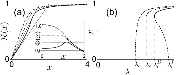
To precisely analyze the nature of the phase transitions for the problem of correlated frequencies and degrees, Coutinho et al. defined the function [249]

$$\Phi(x)=\frac{1}{\lambda},$$ (185)

where $\Phi(x)\equiv\mathcal{R}(x)/x$ and is given by

$$\Phi(x) = (\gamma-2)\left(\frac{\Omega(x)}{k_{\min}}\right)^{2-\gamma}\int_{-1}^{1}dy(1-xy)^{\gamma-3}$$ (186)

$$\times\sqrt{1-y^{2}}\Theta(1-xy)\Theta\left(xy-\frac{k_{\min}-\Omega(x)}{k_{\min}}\right),$$

where $y\equiv[k-\Omega(x)]/(xk)$. The horizontal lines in the inset of Fig. 21 are given by $1/\lambda$ and their intersection with $\Phi(x)$ gives the solutions of the order parameter $r$. To obtain a discontinuous transition, the function $\Phi(x)$ must have a maximum for $x\neq 0$. Since $\lim_{x\rightarrow\infty}\Phi(x)=0$, $\Phi(x)$ must be an increasing function at $x=0$, i.e. it has its maximum value at $x\neq 0$. Thus, since $\left.\partial\Phi(x)/\partial x\right|_{x=0}=0$, a sufficient condition for the existence of a first-order transition is $\left.\partial^{2}\Phi(x)/\partial x^{2}\right|_{x=0}>0$, which is equivalent to [249]

$$\frac{(\gamma-4)(\gamma-3)}{4(\gamma-2)}-\frac{\Omega^{\prime\prime}(0)}{\Omega(0)}>0,$$ (187)

where $\Omega^{\prime\prime}(0)=\left.\partial^{2}\Omega(x)/\partial^{2}x\right|_{x=0}$. Although there is no explicit solution of $\Omega$ as a function of $x$, it is possible to determine its dependence on exponent $\gamma$ for $x$. This dependence is given by [249]

$$\frac{\Omega(0)}{k_{\min}}-2=\frac{\pi^{2}}{4}(\gamma-3),$$ (188)

$$\frac{\Omega^{\prime\prime}(0)}{k_{\min}}\simeq 1.71(\gamma-3)$$ (189)

Inserting Eqs. 188 and 189 into Eq. 187 we obtain the phase diagram depicted in Fig. 22. Notice that three regions are uncovered. Region I is marked by the presence of incoherence, i.e., no synchronous behavior emerges for $\lambda<\lambda_{c}$. Synchronization ($r>0$) takes place in region II, where $\lambda>\lambda_{c}^{\rm{I}}$. Finally, the system will generate a hysteresis for parameters belonging to region III in which one stable and one metastable solution are found. Furthermore, by expanding the function $\Phi(x)$ using Taylor series around $x$ one finds that, for $\gamma=3$, the order parameter follows $r-r_{c}\propto(\lambda-\lambda_{c})^{\beta}$, where $\beta=2/3$, which is the same critical exponent found by Pazó [56] for uniform frequency distributions [249].

Figure 22: Phase diagram of the Kuramoto model with degree-correlated frequencies in SF networks. Area I denotes the region with incoherence, i.e., $r=0$. Synchronization emerges for parameters belonging to area II. The system will present hysteresis in area III, where there is bistability between the incoherent and synchronous state. Adapted with permission from [249]. Copyrighted by the American Physical Society.

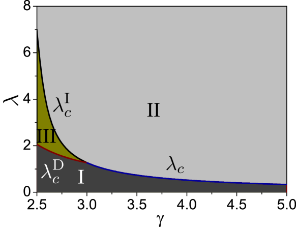
The findings in [249] yield important insights into the dynamics of Kuramoto oscillators with frequencies correlated with degrees in networks without degree-degree correlations. Specifically, it predicts that SF networks with $\gamma>3$ undergo a second-order transition, changing to a hybrid transition at $\gamma=3$ with no hysteresis and finally becoming a first-order transition for $\gamma<3$. However, as remarked by the authors in [249], the result for $\gamma>3$ is in apparent contradiction to those presented by Goméz-Gardeñes et al. [30]. More specifically, in [30] the authors numerically found that SF networks with $\gamma=3.3$ constructed through the CM undergo a first-order transition, in contrast to what is predicted by the calculations in [249]. This inconsistency between both results may be due to finite-size effects presented by networks of size $N=10^{3}$ considered in [30]. It is important to note that networks with finite-size constructed by the CM might exhibit non-vanishing values for the clustering-coefficient and also can have degree-degree correlations [25]. Thus, this makes the assumption of networks in the absence of degree-degree correlations no longer valid leading, in this way, to a different result as the one predicted by diagram in Fig. 22. As we shall see in the next sections, non-vanishing values of the assortativity coefficient can significantly change the synchronization properties of networks under correlation between frequencies and degrees.

Besides analyzing the Kuramoto model for the frequency assignment $\omega_{i}=k_{i}$, Coutinho et al. also studied the model in star graphs [249], i.e., networks made up of a central node connected to $K$ peripheral nodes with degree $k_{j}=1$, for $j=1,...,K$, where $K$ is the total number of peripheral nodes. The equations for the model in the star graph are given by

$$\dot{\theta}_{H}=\omega_{H}+\lambda\sum_{j=1}^{K}\sin(\theta_{j}-\theta_{H}),$$ (190)

$$\dot{\theta}_{j}=\omega_{j}+\lambda\sin(\theta_{H}-\theta_{j}),$$ (191)

where $\theta_{H}$ and $\theta_{j}$ are the phases of the central (or hub) node and the $j$-th peripheral node. By appropriately defining the order parameter as

$$re^{i\psi}=\frac{1}{K}\sum_{j=1}^{K}e^{i\theta_{j}},$$ (192)

it is possible to decouple the Eqs 190 and 191 as

$$\dot{\theta}_{H}-\Omega=(\omega_{H}-\Omega)-\lambda Kr\sin(\theta_{H}-\psi)\mbox{ and}$$ (193)

$$\dot{\theta}_{j}-\dot{\theta}_{H}=(\omega_{j}-\dot{\theta}_{H})-\lambda\sin(\theta_{j}-\theta_{H}).$$ (194)

The hub will be locked when $\dot{\theta}_{H}=\Omega$, satisfying

$$\omega_{H}-\Omega=\lambda Kr\sin(\theta_{H}-\psi),$$ (195)

where $\Omega$ is the common frequency. Furthermore, the locked solution associated to Eq. 191 is given by

$$\omega_{j}-\Omega=\lambda\sin(\theta_{H}-\theta_{j}),$$ (196)

for $\left|\omega_{j}-\Omega\right|<\lambda$. On the other hand, if $\left|\omega_{j}-\Omega\right|>\lambda$ then the $j$-th peripheral node is not entrained by the mean-field. In this way, similarly as in Eq. 179, the contributions to the order parameter can be explicitly written as [249]

$$re^{i(\psi-\theta_{H})}=\frac{1}{K}\sum_{|\omega_{j}-\Omega|\leq\lambda r}e^{i(\theta_{j}-\theta_{H})}+\frac{1}{K}\sum_{|\omega_{j}-\Omega|>\lambda r}e^{i(\theta_{j}-\theta_{H})}.$$ (197)

Considering that the peripheral nodes have identical frequencies so that frequencies and degrees are correlated in the star gaph, i.e. with frequency distribution

$$g(\omega)=\frac{1}{K}\sum_{j=1}^{K}\delta(\omega-\omega_{j}),$$ (198)

one can derive the following implicit equations for $\Omega$ and $r$ [249],

$$r^{2}=\left(\frac{\Omega-\omega_{H}}{K\lambda}\right)^{2}+\left[\int_{-\lambda}^{+\lambda}d\omega g(\omega+\Omega)\sqrt{1-\left(\frac{\omega}{\lambda}\right)^{2}}\right]^{2},$$ (199)

$$\frac{\Omega-\omega_{H}}{K}=\int_{|\omega|>\lambda}d\omega g(\omega+\Omega)\omega\left[1-\sqrt{1-\left(\frac{\lambda}{\omega}\right)^{2}}\right].$$ (200)

The average frequency $\Omega$ should be first determined through Eq. 200, which can then be used to calculate the order parameter $r$ via Eq. 199. As mentioned in [249], if $\omega_{H}-\left\langle\omega_{j}\right\rangle<\omega_{c}$, where $\left\langle\omega_{j}\right\rangle$ is the average frequency of the peripheral nodes and $\omega_{c}$ a certain threshold, the phase transition is continuous and $r$ increases as a function of $\lambda$. On the order hand, if $\omega_{H}-\left\langle\omega_{j}\right\rangle>\omega_{c}$ then the transition becomes discontinuous with the presence of hysteresis in the plane $\lambda-r$. It is interesting to note that the mechanism behind the emergence of abrupt transitions in star graphs is a sufficient large frequency mismatch between the hub and its neighbors. This gives also insights into the dynamics of SF networks with correlation between frequencies and degrees. In their topology hubs can locally form star-like structures leading to a frequency mismatch between oscillators and, consequently, yielding a first-order transition [249, 254].

Zou et al. [254] also addressed the relation between the dynamics of star and SF networks using a different approach, namely by analyzing the basin of attraction of the synchronized state. The authors defined first the state space of Eq. 190 and  191 as a $K+1$ dimensional torus $\mathbb{T}^{K+1}$ [254] , where $K$ is the number of peripheral nodes in the star networks, as previously defined. By setting $\omega_{H}=K\omega$ and $\omega_{j}=\omega$ ($j=1,...,K$) in Eqs.  190 and  191; and defining $\bm{\theta}=(\theta_{1},...,\theta_{K},\theta_{H})$, $\bm{\omega}=(\omega,...,\omega,K\omega)$ and the function $\mathbf{H}:\mathbb{T}^{K+1}\rightarrow\mathbb{T}^{K+1}$ given by $\left(\sin(\theta_{H}-\theta_{1}),\sin(\theta_{H}-\theta_{2}),...,\sin(\theta_{H}-\theta_{K}),\sum_{j=1}^{K}\sin(\theta_{j}-\theta_{H})\right)$, the Eqs.  190 and  191 can be rewritten as

$$\dot{\bm{\theta}}=\bm{\omega}+\lambda\mathbf{H}(\bm{\theta}).$$ (201)

Therefore, the locking manifold is given by

$$M_{a}:=\{\bm{\theta}\in\mathbb{T}^{K+1}:\theta_{1}=\cdots=\theta_{K}\mbox{ and }\theta_{H}-\theta_{1}=a\},$$ (202)

admitting the solutions $\dot{\bm{\theta}}=\bm{\omega}-\lambda\mathbf{H}(\mathbf{a)}$, where $\mathbf{a}=c(1,...,1)+(0,...,0,a)$, with $c$ being a constant real number, leading to $\bm{\theta}(t)=\left[\bm{\omega}-\lambda\mathbf{H}(\mathbf{a})\right]t+\bm{\theta}_{0}$, where $\bm{\omega}_{0}\in M_{a}$, and satisfying

$$-(K-1)\omega+\lambda(K+1)\sin a=0.$$ (203)

Equation 203 is valid for $(K-1)\omega/(K+1)\lambda\leq 1$, which yields the critical coupling $\lambda_{c}^{\rm{D}}$ for the backward continuation [254]:

$$\lambda_{c}^{\rm{D}}=\frac{(K-1)\omega}{K+1}.$$ (204)

For $\lambda>\lambda_{c}^{\rm{D}}$ and using the solutions provided by the locked manifold in Eq. 202, one can get the full dependence of the order parameter $r$ as a function of $\lambda$, which is given by

$$r^{2}=\frac{K^{2}+1}{(K+1)^{2}}+\frac{2K}{(K+1)^{2}}\sqrt{1-\left[\frac{(K-1)\omega}{(K+1)\lambda}\right]^{2}},$$ (205)

which for $\lambda=\lambda_{c}^{\rm{D}}$ yields [254]

$$r_{c}^{\rm{D}}=\frac{\sqrt{K^{2}+1}}{K+1}.$$ (206)

Equation 206 gives the critical value of the order parameter at the transition point for the backward propagation. The comparison between the theoretical results in Eq. 204 and 206 and numerical simulations are shown in Fig. 23. Noteworthy, the expression for $r_{c}^{\rm{D}}$ obtained in [254] differs from the one calculated in the original paper by Gómez-Gardeñez et al. [30], where the authors obtained $r_{c}^{\rm{D}}=K/(K+1)$, considering $\omega=1$. However, if we tend the number of peripheral nodes to zero ($K\rightarrow 0$), one expects to obtain perfect synchronization in the system composed only by a central node. This condition is included by the order parameter in Eq. 206, but not by the result presented in [30].

Figure 23: (a) The order parameter $r$ as a function of coupling $\lambda$ for star-graphs with $K=5$ and $40$ and (b) $K=10$. Branch II corresponds to the dynamics without the inclusion of disorder $\zeta_{j}$, whereas I and III the frequencies of the peripheral nodes are given by $\omega_{j}=\omega+\zeta_{j}$, where $\zeta_{j}\in[-0.05,0.05]$. Adapted from [254].

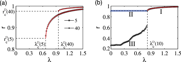
In order to determine the conditions for synchronization for the case in which the coupling strength is adiabatically increased, one should notice that the locking manifold $M_{a}$ in Eq. 202 is locally attractive for $\lambda\in[\lambda_{c}^{\rm{D}},\lambda_{c}^{\rm{I}}]$. Thus, as the coupling increases, $M_{a}$ becomes globally attractive for $\lambda>\lambda_{c}^{\rm{I}}$, i.e., any incoherent state for $\lambda>\lambda_{c}^{\rm{I}}$ is attracted to the manifold $M_{a}$. Using this information and the theory developed in [260, 261], one gets that the critical coupling for the forward propagation is given by [254]

$$\lambda_{c}^{\rm{I}}\thickapprox\left(\frac{K-1}{B\sqrt{K}}\right)\omega,$$ (207)

where $B$ is a constant that depends on the initial conditions [254]. As we can see, Eq. 207 shows that the onset of synchronization in a star-graph increases with the system size. This dependence was also numerically observed in the original paper by Gómez-Gardeñez et al. [30].

As previously mentioned, the analysis of the dynamics in star-graphs has the potential to qualitatively describe the emergence of explosive synchronization in SF networks, since the latter can be regarded as a collection of interconnected hubs [249, 254]. Hubs and their low-degree neighbors form locally star-like structures creating, in this way, local locking manifolds as in Eq. 202. In fact, the result in Eq. 207 can be used to estimate the critical coupling of SF networks with degree distributions $P(k)\sim k^{-\gamma}$. The maximum degree for a SF network with the critical exponent $\gamma$ scales as $k_{\max}\propto N^{\frac{1}{\gamma-1}}$ [25]. Therefore, using Eq. 207 and considering an average of a network ensemble, one obtains the scaling relation

$$\left\langle\lambda_{c}^{\rm{I}}\right\rangle\propto N^{\frac{1}{2(\gamma-1)}}.$$ (208)

In order to sustain this hypothesis, Fig. 24(a) shows the local order parameter $r_{i}$ of two hubs in a SF network generated by the BA model with $N=2000$ and $\left\langle k\right\rangle=2$. As we can see, the parameters $r_{i}$ also undergo discontinuous phase transitions as a function of $\lambda$ and also agree with the limit $\lambda_{c}^{\rm{D}}\rightarrow\omega$, for $K\gg 1$ in Eq. 204. Furthermore, in Fig. 24 (b) we see a good agreement between the scaling relation predicted in Eq. 208 and the simulation results.

Figure 24: (a) The local order parameter $r_{i}$ as a function of coupling $\lambda$ of two hubs selected from a BA network with $N=2\times 10^{3}$ nodes and average degree $\left\langle k\right\rangle=2$. Red curve: hub with degree $K_{1}=39$; blue curve: hub with degree $K_{2}=24$. (b) Critical coupling $\left\langle\lambda_{c}^{\rm{I}}\right\rangle$ of the forward propagation of $\lambda$ as a function of network size $N$. $\left\langle\cdot\right\rangle$ denotes an average over 50 different network realizations. Adapted from [254]. Copyrighted by the American Physical Society.

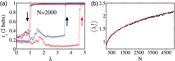
Noteworthy, alternative solutions for the synchronization of star graphs with frequency-degree correlations were recently proposed in [262] using the Wattanabe-Strogatz approach [263, 264, 172, 265], and in [266], where the OA theory was employed. The corresponding stability analysis revealed that only positive correlation between the frequencies and degrees yields discontinuous transitions in star-graphs. In particular, it was demonstrated that, for the forward propagation of coupling $\lambda$, after reaching the critical coupling $\lambda_{c}^{\rm{I}}$ the asynchronous state loses its stability, being replaced by the fixed point related to the synchronized state [262].

Before reviewing other different types of correlations between topology and intrinsic dynamics introduced in the literature, it is interesting to analyse situations in which the system is perturbed by properties found in real applications. First, we consider when the condition $\omega_{i}=k_{i}$ is slightly disturbed by random fluctuations. Zou et al. [254] also investigated the dynamics of star-graphs whose phases of the peripheral nodes evolve according to

$$\dot{\theta}_{i}=\omega+\zeta_{i}+\lambda\sin(\theta_{H}-\theta_{i}),\;(i=1,...,K),$$ (209)

where $\zeta_{j}$ is a variable randomly drawn from a uniform distribution in the range $\left[-\varepsilon,\varepsilon\right]$. Note that only the hub is not subjected to a random frequency perturbation. Regarding the backward propagation of coupling $\lambda$, it was verified that for $\lambda>\lambda_{c}^{\rm{D}}$ the locking manifold $M_{a}$ is not destroyed by such random fluctuations, once the magnitude of fluctuation $\varepsilon$ is small enough (see region I in Fig. 23(b)). On the other hand, for values of coupling $\lambda<\lambda_{c}^{\rm{D}}$ the manifold $M_{a}$ is destroyed leading the peripheral nodes to oscillate incoherently at different frequencies, as seen in branch III in Fig. 23(b). The comparison with the dynamics in the absence of disorder is shown in branch II of the same figure.

Figure 25: Synchronization diagram of the forward (fw) and backward (bw) propagation for SF networks with $N=1000$ for (a) $\varepsilon=0$ and (b) $\varepsilon=20$. Panels (c) and (d) correspond to the theoretical curves of simulations in (a) and (b), respectively. All networks have $\gamma=3.5$ and $k_{\min}=10$. Reprinted with permission [248]. Copyright 2014 by the American Physical Society.

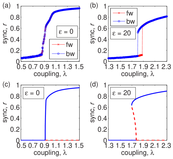
The effect of addition of disorder to disturb the frequency assignment $\omega_{i}=k_{i}$ was further analyzed by Skardal and Arenas  [248] for more heterogeneous structures, namely for SF and stretched exponential networks with a degree distribution given by $P(k)\propto k^{b-1}\exp[-\left(k/\mu\right)^{b}]$. As shown in  [249], SF networks with $\gamma>3$ no longer exhibit discontinuous phase transitions. However first-order transitions can be induced for cases in which the phase transitions are continuous under the condition $\omega_{i}=k_{i}$ if $\varepsilon$ is large enough [248]. The effect of addition of disorder on the order parameter $r$ can be seen in Fig. 25 for a network with $\gamma=3.5$. For $\varepsilon=0$ (Fig. 25(a)) the transition is continuous, as predicted in the theoretical curve in Fig. 25(c). Yet, when $\varepsilon$ is increased to $\varepsilon=20$, a discontinuous phase transition with the presence of hysteresis emerges, as it is seen in the simulation in Fig. 25(b) and the respective theoretical curve in Fig.  25(d). It is interesting to note also that explosive synchronization as an effect of inclusion of quenched disorder only arises for strong values of $\varepsilon$. More precisely, for less heterogeneous networks, even with perfect correlation between frequencies and degrees, explosive synchronization is not observed. The disorder introduced in the system must overcome this homogeneity in the network structure so that the order parameter exhibits discontinuity. However, the larger the strength of disorder $\varepsilon$, the weaker the influence of degrees in the overall frequency $\omega_{i}=k_{i}+\zeta_{i}$. Therefore, if the magnitude of fluctuation $\varepsilon$ is sufficiently large, the frequency distribution is nearly uniform, leading to an analogous case as earlier considered by Pazó [56].

Another scenario found in many real-world systems is that the interaction between the dynamical units may not occur instantaneously, but rather only after a time delay [267] (see also Sec. 4.1). Peron and Rodrigues [243] numerically investigated the Kuramoto model in time-delayed networks

$$\dot{\theta}_{i}(t)=\omega_{i}+\lambda\sum_{j=1}^{N}A_{ij}\sin\left[\theta_{j}(t-\tau)-\theta_{i}(t)\right],$$ (210)

where $\omega_{i}=k_{i}$ and $\tau$ is the time delay. The synchronization diagram considering BA networks is shown in Fig. 26. It is interesting to observe how the coherence of the populations of oscillators as a function of coupling dramatically changes when a time delay is included in the system. Even small values of $\tau$ are able to decrease the critical coupling, enhancing in this way the synchronization. Furthermore, besides enabling the network to reach the synchronous state for lower coupling strengths, the inclusion of a time delay also modifies the type of the phase transition. For instance, for $\tau=1$, a discontinuous transition is obtained (similarly as in the original case with $\tau=0$), while for $\tau=2$, the system exhibits a continuous transition. It is also worth noting that some choices of $\tau$, namely $\tau=0.1$ and $0.5$, yield non-usual scaling of the order parameter for lower values of the coupling strength. The authors in  [243] analytically studied the dynamics in star-graphs, which qualitatively explains the dependency of the order parameter observed in Fig. 26. However, the mean-field solution of the model (210) for degree-correlated frequencies in SF networks is still open. In fact, the detailed investigation of such a problem could yield insights into real applications in which the hysteric behavior can be avoided by the addition of time delay in the communication of the dynamical units.

Figure 26: The order parameter $r$ vs. coupling strength $\lambda$ for SF networks with $\gamma=-3$ and $N=10^{3}$ oscillators considering different time delays $\tau$. Reprinted with permission from [243]. Copyright 2012 by the American Physical Society.

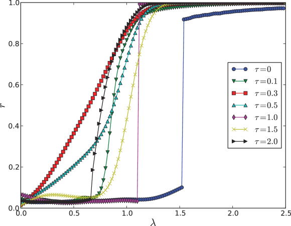
5.2 Other kinds of correlations

Naturally the results by Gómez-Gardeñes et al. [30] raised many questions regarding the dynamics of Kuramoto oscillators in networks. Of particular interest is the problem of whether other types of correlations between topology and intrinsic dynamics of the oscillators also lead to discontinuous synchronization transitions.

For instance, Skardal et al. [253] analyzed the Kuramoto model in uncorrelated networks where the frequencies and degrees are subject to the following joint probability distribution

$$P(k,\omega)=\frac{P(k)}{2}\left[\delta(\omega-ak^{b})+\delta(\omega+ak^{b}\right)],$$ (211)

i.e., the frequency of oscillator $i$ is $\omega_{i}=\pm ak_{i}^{b}$. For the original case in which $a=b=1$ and only positive frequencies are considered, the correlation between frequencies and degrees in [30] is recovered. The model subjected to correlation between frequencies and degrees imposed by Eq. 211 exhibits significant different properties compared to the one in [30]. Specifically, Fig. 27(a) shows the order parameter $r$ (Eq. 23) as a function of coupling $\lambda$ for an ER network. One can identify three different regimes, namely (i) incoherent state, (ii) standing wave and (iii) stationary state [253]. State (i) is characterized by the absence of synchronization for $\lambda<\lambda_{1}$. In the (ii) regime, a spontaneous drift of the order parameter $r$ appears resulting in a time dependent behavior observed in Fig. 27(b) (the phase distribution $\rho(\theta)$ for two extreme values of $r$ can be seen in Fig. 27(c)). On the other hand, for $\lambda>\lambda_{2}$ the (iii) regime is reached for which the order parameter $r$ is time-independent, as shown in Fig. 27(d).

Figure 27: Numerical analysis of the Kuramoto model in an ER network with correlation between frequencies and degrees given by Eq. 211 with $N=10^{3}$ and $\left\langle k\right\rangle=10$. (a) Time-averaged order parameter $R$ as a function of coupling $\lambda$. (b) Order parameter $R$ as a function of time for $\lambda=1.9$ and (c) the phase distribution $\rho(\theta)$ for points in red and green in panel (b). (d) Order parameter as a function of $t$ for $\lambda=2.1$. Here, the acronyms I, SW and SS stand for incoherent, standing wave and stationary state, respectively. Adapted with permission from [253].

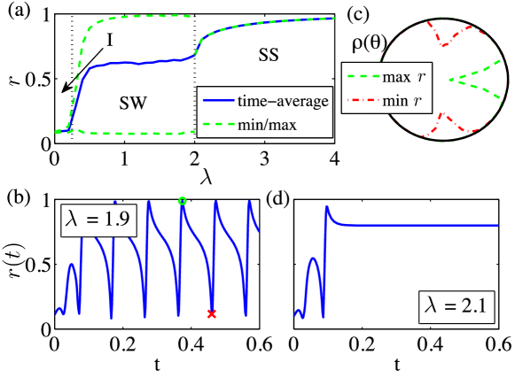
Besides the standing wave state induced by the bimodal distribution in Eq. 211, the connectivity pattern of the entrained oscillators strongly varies depending on the exponent $b$. More specifically, for $b<1$ (sublinear) high degree nodes will form a synchronized component in the network, while the drifting oscillators will be mostly composed of low degree nodes. This scenario inverts for $b>1$ (super-linear), i.e., the synchronized cluster is now dominated by low degree nodes. For the linear correlation regime, $b=1$, the stationary state is characterized by a full locking, i.e., the absence of drifting oscillators.

In order to get analytical insights into this behavior, it is convenient to define the order parameters for positive and negative frequencies as $r_{i}^{\pm}e^{i\psi^{\pm}}=\sum_{\omega_{j}\lessgtr 0}A_{ij}e^{i\theta_{j}}$ and $r^{\pm}=\frac{1}{N}\sum_{j=1}^{N}r_{j}^{\pm}/k_{j}^{\pm}$, where $k_{j}^{\pm}$ is the degree of node $j$ due to connections with nodes with positive (resp. negative) frequencies. Using these definitions, the equations of motion can be decoupled as

$$\dot{\theta}_{i}=\omega_{i}+\lambda\left[r^{+}_{i}\sin(\psi_{i}^{+}-\theta_{i})+r^{-}_{i}\sin(\psi_{j}^{-}-\theta_{i})\right].$$ (212)

Setting the rotating frame $\phi_{i}=\theta_{i}-\Omega t$ and defining $\psi_{i}^{\pm}=\pm\Omega t$, the equations of motion can be rewritten as

$$\dot{\phi}_{i}=(\omega_{i}-\Omega)-\lambda r^{+}_{i}\sin\phi_{i}-\lambda r_{i}^{-}\sin(\phi_{i}+2\Omega t).$$ (213)

Imposing the phase-locked solution $\dot{\phi}_{i}=0$, we get the following relations [253]

$$r^{+}=\frac{1}{\left\langle k\right\rangle}\int_{2\left|ak^{b}-\Omega\right|\leq\lambda r^{+}k}P(k)k\sqrt{1-\frac{4\left(ak^{b}-\Omega\right)^{2}}{\left(\lambda r^{+}k\right)^{2}}},$$ (214)

$$\Omega=a\frac{\int_{2\left|ak^{b}-\Omega\right|\leq\lambda r^{+}k}P(k)k^{b}dk}{\int_{2\left|ak^{b}-\Omega\right|\leq\lambda r^{+}k}P(k)dk},$$ (215)

which are also satisfied by replacing $r^{+}\rightarrow r^{-}$ [253]. Furthermore, for the SS regime, i.e. for $\Omega=0$, Eq. 214 reduces to

$$r=\frac{1}{\left\langle k\right\rangle}\int_{ak^{b}\leq\lambda rk}P(k)k\sqrt{1-\left(\frac{ak^{b}}{\lambda rk}\right)^{2}}dk.$$ (216)

From Eq. 216 it becomes clear that the three possible regimes are induced in dependence on the parameter $b$. Specifically, for $b>1$ oscillators with degree $k\leq\left(\frac{\lambda r}{a}\right)^{\frac{1}{b-1}}$ become entrained by the mean-field, whereas the oscillators with higher degrees become drifting. For $b<1$ the range of degree of the synchronized oscillators is given by $k\geq\left(\frac{a}{\lambda r}\right)^{\frac{1}{1-b}}$. On the other hand, if $b=1$, the dependence on $k$ in Eq. 216 is lost and all oscillators become locked, once the critical coupling is reached and $\Omega=0$.

The emergence of discontinuous synchronization transitions has been described as an effect exclusively due to the microscopic correlation between dynamics and local topology. This now poses the question of whether abrupt transitions can be observed in networks where the constraint $\omega_{i}\propto k_{i}$ does not hold and what would be the necessary conditions for the existence of such dynamical behavior in networks. One of the first steps towards the understanding of this problem was given by Leyva et al. [268]. The authors remarked that, in order to obtain a discontinuity in the order parameter as a function of coupling, one should avoid a smooth emergence of a giant synchronous components. With this hypothesis Leyva et al. elaborated the condition for frequency assignment stating that every pair of nodes should satisfy [268]

$$|\omega_{i}-\omega_{j}|>\varepsilon_{c}.$$ (217)

More specifically, the condition (217) inhibits the formation of small synchronous clustering by imposing a gap in the frequency mismatch or, in other words, a frequency dissortativity. Figure 28 shows simulations with ER networks created following Eq. 217. As we can see in Fig. 28(a), for sufficient large $\varepsilon$ the transition becomes discontinuous, a phenomenon not observed for the same network topology under the constraint $\omega_{i}=k_{i}$ [30, 242, 249]. Moreover, it is interesting to note in Figs. 28(c) and (d) that a correlation between frequencies and degrees naturally emerges by imposing the frequency mismatch beforehand. Figs. 28 (e) and (f) further show the calculation of the critical mismatch $\varepsilon_{c}$ for $\left\langle k\right\rangle=20$ and $60$, respectively.

Figure 28: Synchronization diagrams for networks satisfying condition in Eq. 217 for (a) $\left\langle k\right\rangle=40$ and different values of threshold $\gamma$, (b) $\varepsilon=0.4$ and varying average degree $\left\langle k\right\rangle$. Solid (dashed) lines stand for the forward (backward) propagation of coupling $\lambda$. (c) Scatter plots of the degrees $k_{i}$ against frequencies $\omega_{i}$ in a network constructed under condition in Eq. 217 with $\left\langle k\right\rangle=100$ and frequency mismatch $\varepsilon=0$; and (d) $\varepsilon=0.4$. Parameter space $\lambda-\varepsilon$ coloured according the order parameter $r$ for (e) $\left\langle k\right\rangle=20$ and (f) $\left\langle k\right\rangle=20$. All networks have $N=500$ oscillators. Reprinted by permission from Macmillan Publishers Ltd: Scientific Reports [268], copyright 2013.

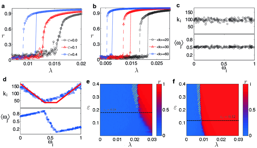
Interestingly, it is possible to relax the condition in Eq. 217, while preserving the discontinuity of the order parameter. More specifically, it was shown that condition (217) can be softened to

$$|\omega_{i}-\left\langle\omega_{j}\right\rangle|>\varepsilon_{c},$$ (218)

where $\left\langle\cdots\right\rangle$ stands for the average over the neighbours of node $j$ [268]. Thus, Eq. 218 imposes that two nodes $i$ and $j$ will be connected only if the difference between frequency $\omega_{i}$ overcomes the local mean-field of the neighborhood of the node $j$. As in the case of Eq. 217, a spontaneous emergence of correlation between frequencies and degrees is observed [268]. Remarkably, the condition in Eq. 218 imposed in [268] is exactly the same condition $|\omega_{i}-\left\langle\omega_{j}\right\rangle|>\omega_{c}$ analytically found to obtain first-order transitions in star-graphs [249].

Motivated by these findings that explosive synchronization is achievable for any frequency distributions, Leyva et al. [251] further analysed the following model

$$\dot{\theta}_{i}=\omega_{i}+\frac{\lambda}{\left\langle k\right\rangle}\sum_{j=1}^{N}\Gamma_{ij}^{\varsigma}\sin(\theta_{j}-\theta_{i}).$$ (219)

The frequencies $\omega_{i}$ are distributed according to a frequency distribution $g(\omega)$ and the link weights are given by

$$\Gamma_{ij}^{\varsigma}=A_{ij}\left|\omega_{i}-\omega_{j}\right|^{\varsigma},$$ (220)

The interactions between the oscillators depend now on the frequency mismatch, however without imposing any frequency dissortativity as in Eqs. 217 and 218. Figure 29(a) shows the synchronization diagram calculated by numerically evolving the equations (219) for several choices of distribution $g(\omega)$ and considering an ER network with $N=500$ nodes and $\left\langle k\right\rangle=15$. It is interesting to note that the transition is second-order for a uniform distribution $g(\omega)$ and $\varsigma=0$, whereas for $\varsigma=1$ with the same $g(\omega)$ the transition becomes discontinuous. Furthermore, once the range of frequencies is kept fixed ($\omega\in[0,1]$), the dependence of the order parameter $r$ on $\lambda$ remains unchanged.

Figure 29: (a) Order parameter $R$ (Eq. 2) as a function of $\lambda$ for the model defined in Eq. 219 considering $N=500$, $\left\langle k\right\rangle=30$ and different values of exponent $\varsigma$ and different choices for frequency distribution $g(\omega)$ in the range $[0,1]$. Solid (dashed) lines correspond to the forward (backward) propagation of coupling $\lambda$. (b) Scatter plots of the nodes’ strength $s_{i}=\sum_{j}A_{ij}\left|\omega_{i}-\omega_{j}\right|^{\varsigma}$ vs. natural frequency $\omega_{i}$, where dark blue squares and circles correspond to the cases $\varsigma=0$ and $\varsigma=1$, respectively, for uniform frequency distribution in panel (a). Solid line represents the analytical prediction $s\sim\left(\omega-\frac{\varepsilon}{2}\right)^{2}+\frac{1}{4\varepsilon}$ (Eq. 225) for $\varepsilon=1$. Adapted with permission from [251]. Copyrighted by the American Physical Society.

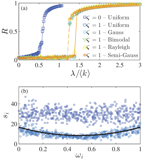
Introducing the weights $\Gamma_{ij}^{\varsigma}$ also naturally induces a correlation between the nodes strengths $s_{i}$ and the natural frequencies $\omega_{i}$, as seen in Fig. 29(b). The correlation $s_{i}\sim\omega_{i}$ spontaneously emerges as a consequence of the weighting procedure [251], in contrast with the correlation between frequencies and degrees considered in [30], where such constraint is imposed in order to yield discontinuous transitions. In fact, the dependence of $s$ on $\omega$ can be explicitly obtained for a fully connected graph. Thus, considering the model

$$\dot{\theta}_{i}=\omega_{i}+\frac{\lambda}{N}\sum_{j=1}^{N}\left|\omega_{i}-\omega_{j}\right|\sin(\theta_{j}-\theta_{i}),$$ (221)

one can express the equations as [251]

$$\dot{\theta}_{i}=\omega_{i}+\lambda r_{i}\sin(\psi_{i}-\theta_{i}),$$ (222)

where $r_{i}$ and $\psi_{i}$ are the amplitude and the phase of the local mean-field, respectively; i.e.,

$$r_{i}e^{i\psi_{i}}=\frac{1}{N}\sum_{j=1}^{N}\left|\omega_{i}-\omega_{j}\right|e^{i\theta_{j}}.$$ (223)

The stationary solution in the continuum limit gives $\omega=\lambda r(\omega)\sin[\theta(\omega)-\psi(\omega)].$ By defining the functions

$$F(\omega)=r(\omega)\sin\psi(\omega)=\int g(y)\left|\omega-y\right|\sin\theta(y)dy,$$

$$G(\omega)=r(\omega)\cos\psi(\omega)=\int g(y)\left|\omega-y\right|\cos\theta(y)dy,$$

Eq. 222 in the stationary state is rewritten as

$$\frac{2}{\lambda}g(\omega)\omega=G(\omega)\frac{d^{2}F(\omega)}{d\omega^{2}}-F(\omega)\frac{d^{2}G(\omega)}{d\omega^{2}}.$$ (224)

Noting that $G(\omega)\approx rs(\omega)$ when the system is close to the synchronous state and considering a uniform frequency distribution $g(\omega)$ in the range $\omega\in[-\varepsilon/2,\varepsilon/2]$, the obtained strength $s$ is

$$s(\omega)=\varepsilon\left[\left(\frac{\omega}{\varepsilon}\right)^{2}+\frac{1}{4}\right],$$ (225)

which is the black curve depicted in Fig. 29(b). Moreover, the order parameter $r$ can also be obtained analytically determined in a similar way as previously. More specifically, it can be shown that in the case of the model in Eq. 221 for uniform frequency distribution defined in the range $\omega\in[-\varepsilon/2,\varepsilon/2]$, the order parameter is given by

$$r=\int_{-\frac{\varepsilon}{2}H^{-1}(\lambda r)}^{\frac{\varepsilon}{2}H^{-1}(\lambda r)}g(\omega)\sqrt{1-\left[\frac{1}{\lambda r}H\left(\frac{2\omega}{\varepsilon}\right)^{2}\right]}d\omega,$$ (226)

where $H(y)$ is the function

$$H(y)=\frac{4}{4+\pi}\left[\frac{y}{1+y^{2}}+\arctan(y)\right].$$ (227)

Solving Eq. 226 one gets the full dependence of the parameter $r$ on the coupling $\lambda$.

Figure 30: Order parameter $R$ (Eq. 2) as a function of coupling $\lambda$ of model defined in Eq. 228 considering the fully connected graph with (a) Lorentzian and (b) Gaussian frequency distribution. Panels (c) and (d) correspond to the cases of an ER and SF network, respectively, with Lorentzian frequency distribution and average degree $\left\langle k\right\rangle=6$. Adapted with permission from [245]. Copyrighted by the American Physical Society.

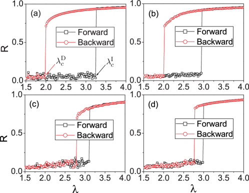
Analyzing the variations of the Kuramoto model discussed in this section we notice that having frequencies proportional to degree is just one of the possible mechanisms that can lead to abrupt transitions either in networks or in fully connected graphs. Another example is the model considered by Zhang et al. [245], which consists of a system governed by the following equations

$$\dot{\theta}_{i}=\omega_{i}+\frac{\lambda\left|\omega_{i}\right|}{k_{i}}\sum_{j=1}^{N}A_{ij}\sin(\theta_{j}-\theta_{i}),$$ (228)

where $\omega_{i}$ are drawn from a distribution $g(\omega)$. Instead of directly correlating dynamics and topology, the model considered in [245] includes an asymmetric coupling between oscillators that is proportional to the individual natural frequencies. In Fig. 30 the synchronization diagram of model by (228) is presented for different frequency distributions $g(\omega)$ and network topologies. Specifically, Fig. 30(a) and (b) consider oscillators in a fully connected graph with Lorentzian and Gaussian frequency distribution, respectively. As seen there, the nature of the transition is not affected by the choice of $g(\omega)$ (see also [269] for investigations of model (228) considering asymmetric frequency distributions). The same effect is observed if the topology of the networks is varied, as depicted in the panels (c) and (d), where the authors considered ER and SF networks constructed through the CM. The only exception reported by the authors in [245] in which the synchronization transition becomes continuous is obtained for $g(\omega)=\sqrt{\frac{2}{\pi}}\exp\left(-\frac{\omega^{2}}{2}\right)$ and $\omega>0$. Noteworthy, nonlinear frequency-weighted couplings have also been considered [270, 271], where, besides asynchronous and synchronous states, oscillatory and chimera states were reported to occur depending on the weighting exponent.

5.3 The role of degree-degree correlations

We saw that one of the key mechanisms to induce a discontinuous synchronization transition networks of Kuramoto oscillators is the existence of sufficient large frequency mismatches between nodes and their neighbors (see Eqs. 217 and 218)  [268, 249]. In fact, the original correlation between frequencies and degrees considered by Gómez-Gardeñez et al. [30] fits this frequency dissortativity condition for SF networks. Based on the analysis of star-graphs and on the assumption that they are building blocks for SF networks, the fulfillment of this condition qualitatively explains the routes to explosive synchronization in such structures, as analysed in Sec. 5.1. Thus, these results suggest that the type of the synchronization transition might strongly depend on the assortative properties of the underlying network.

Analyzing the aforementioned conditions for the occurrence of discontinuous transitions, one expects that the lower the assortativity coefficient of the network, the larger the hysteretic behavior of the order parameter as a function of the coupling strength. By investigating the synchronization of SF networks with a tunable assortativity coefficient using the algorithm described in [106], it was shown in [141] that the hysteresis area decreases in strongly dissortative networks. Apparently this is in contrast with the assumption that larger frequency mismatches, and consequently negative degree-degree correlations, contribute to enhance the irreversibility of the phase transition. However, as remarked in [254], SF networks can be considered as a collection of star graphs only for a sufficient low average degrees or when the network possess locally-tree like structure, i.e., without the presence of loops. Otherwise, the approximation of considering SF network as interconnected star-graphs does not hold, explaining the apparent contradictory result obtained in [141]. In fact, for assortativity values $\mathcal{A}<-0.35$ the synchronization transition is no longer discontinuous for the considered networks. Furthermore, as also discussed in Sec. 3.2, the critical coupling $\lambda_{c}$ was observed to be positively correlated with the network assortativity [141].

Figure 31: Area of hysteresis defined in the synchronization diagram by the forward and backward propagation of coupling strength as a function of the assortativity coefficient $\mathcal{A}$ for (left) growing SF networks constructed via the preferential attachment (PA) rule with initial attractiveness [272] and (right) networks statically generated through the CM. Each point consists in an average over 10 different network realizations. Network parameters are $N=10^{3}$ and $\left\langle k\right\rangle=6$. Adapted with permission from [142]. Copyrighted by the American Physical Society.

The irreversibility of the phase transition was further investigated in [142]. The hysteric behavior of the order parameter is maximized for positive values of the assortativity coefficient $\mathcal{A}$ in growing SF networks, as shown in Fig. 31(a) for different exponents $\gamma$. Surprisingly, networks statically constructed with the very same size $N$, average degree $\left\langle k\right\rangle$ and exponent $\gamma$ through the CM do not present the same dependency on $\mathcal{A}$ as observed in Fig. 31(a) [142]. In this case, the hysteresis is maximized for slightly negative values of $\mathcal{A}$, besides having significant lower values (Fig. 31(b)). This interesting phenomenon was explained in [142] by studying the average betweenness centrality among the highest connected hubs as a function of the degree-mixing. It was found that hubs belonging to networks constructed through growing processes exhibit significant higher betweenness centrality than those in networks generated by the CM. In other words, in growing SF networks, the hubs segregate more efficiently the low-degree nodes, whereas in the CM the highly connected nodes are more homogeneously distributed throughout the network. Thus, since explosive synchronization is induced by the large frequency gaps between neighbors, frustrating in this way the paths to synchronization [142, 268, 273], growing SF networks are more vulnerable to have paths frustrated by such gaps, explaining the higher irreversibility in the transition than in the CM. Furthermore, as the networks are rewired towards extreme values of positive or negative assortativity $\mathcal{A}$, other topological properties, such as average shortest path length, clustering coefficient and even modular structure [106], are dramatically changed up to a point that the frequency gap is not sufficient to yield an abrupt formation of a synchronous giant component [142, 268].

Other works analyzed the effect of non-vanishing assortativity values on the synchronization transition under frequency-degree correlations [140, 138]. For instance, Liu et al. [140] considered natural frequencies to be non-linearly correlated with degrees in the form $\omega=k_{i}^{a}/b$, similarly as in Eq. 211. The authors found that in assortative networks the nodes no longer join abruptly a giant synchronized group, but instead a hierarchical synchronization transition settles in [140]. This is in agreement with the properties described above. Noteworthy, similar dependencies of the nature of the phase transition on degree-mixing properties were also observed in the synchronization of networks made up of FitzHugh-Nagumo oscillators with correlation between intrinsic dynamics and local topological properties [250].

5.4 Other works

Further properties of synchronization in the presence of correlations between the intrinsic dynamics of the oscillators and their local topology were investigated in [255, 274, 275] as well as the dynamics in other types of networks, such as in modular [139] and in co-evolving [246] ones. The effects of partially correlating frequencies and degrees were also investigated [256]. Moreover, of particular interest is the case analysed in [181]. The authors posed the question whether explosive synchronization is achievable without the presence of any kind microscopic correlation in the model. To investigate this issue, networks with adaptive coupling following

$$\dot{\theta}_{i}=\omega_{i}+\lambda\kappa_{i}\sum_{j=1}^{N}A_{ij}\sin(\theta_{j}-\theta_{i}),$$ (229)

were considered, where $\kappa_{i}$ is the coupling parameter. A fraction $f$ of the oscillators is then chosen to have $\kappa_{i}=r_{i}/k_{i}$, where $r_{i}$ is the local order parameter defined in Sec. 2, while for the other fraction $(1-f)$, $\kappa_{i}=1$ is set. Investigating $r$ as a function of coupling $\lambda$, it was found that, after a critical fraction $f_{c}$ is crossed, the networks reach the synchronized state through a discontinuous transition, regardless the network topology or the frequency distribution $g(\omega)$. The same result is obtained when a single-layer network is replaced by a two-layer network. Again, the parameter controlling the emergence of discontinuity of $r$ is the fraction $f$ of oscillators with adaptive coupling $\kappa_{i}=r_{i}$. The findings in [181] reinforced the idea that the necessary condition for the emergence of explosive synchronization is not the correlation between topology and intrinsic dynamics in networks nor a sufficient frequency mismatch among the oscillators, but rather the existence of any suppressive rule that impedes the formation of a giant synchronous component.

Finally, it is also important to mention that the particular frequency assignment introduced by Gómez-Gardeñez et al. [30] has been not only studied in networks of Kuramoto oscillators. In fact, the effects of degree-correlated frequencies were also investigated in networks made up of Rössler [247], FitzHugh-Nagumo [250] and Stuart-Landau [276, 277] oscillators, as well as in experiments with chemo-mechanical oscillators [278].

6 Stochastic Kuramoto Model

The traditional Kuramoto model under the influence of stochastic forces has been already extensively analyzed in many seminal papers, dating back the initial approach by Strogatz and Mirollo [279] and others as [280] and [281]. The precise revision of the early works on the stochastic Kuramoto model in the fully connected graph lies beyond the scope of this review. For such purpose we refer to [4]. Here, nonetheless, we focus on the discussion of the works which are particularly devoted to the analysis of the stochastic model in complex networks. Despite the vast literature on synchronization of stochastic Kuramoto oscillators [4], studies on complex topologies have only been presented very recently [67, 143, 86, 282, 283]. This fact comes as a surprise given the many possible scenarios and applications arising from the interplay between network topology and stochastic dynamics. In this section we present the formulation of the stochastic Kuramoto model in networks and derive the corresponding nonlinear Fokker-Planck equation (FPE) through which the critical coupling strength for the onset of synchronization is obtained. Furthermore, we analyse the low-dimensional behavior of the model using the framework provided by the Gaussian Approximation (GA) technique as well as its generalization to excitable systems described by the Shinomoto-Kuramoto model.

6.1 Onset of synchronization

Sonnenschein and Schimansky-Geier [67] investigated the stochastic Kuramoto model by taking all-together the mean-field approaches in uncorrelated networks [60] with the known results on the stability of the incoherent state in the fully connected graph [279]. More specifically, they considered networks in the absence of degree correlations whose oscillators evolve according to the following equations of motion

$$\dot{\theta}_{i}=\omega_{i}+\frac{\lambda}{N}\sum_{j=1}^{N}A_{ij}\sin\left(\theta_{j}-\theta_{i}\right)+\xi_{i}(t),$$ (230)

where the effect of noise is brought into the model by the terms $\xi_{i}(t)$, which account for the contribution of different stochastic forces. Note the choice made by the authors to include the size of the network $N$ as a normalization term in order to obtain an intensive coupling. This approach differs from those ones adopted in most of the works discussed here, where the commonly adopted coupling is simply $\lambda_{ij}=\lambda$ $\forall i,j$. The terms $\xi_{i}(t)$ are assumed to be sources of Gaussian white noise satisfying

$$\left\langle\xi_{i}(t)\right\rangle = 0,$$

$$\left\langle\xi_{i}(t)\xi_{j}(t)\right\rangle = 2D\delta_{ij}\delta(t-t^{\prime}),$$ (231)

Using the annealed network approximation for the expected value of the adjacency matrix elements in uncorrelated networks, i.e., $\tilde{A}_{ij}=k_{i}k_{j}/\sum_{m}k_{m}$ (see the discussion in Sec. 2.1) and using the order parameter defined in Eq. 35, the equations (230) can be decoupled as

$$\dot{\theta}_{i}=\omega_{i}+r\lambda\frac{k_{i}}{N}\sin(\psi-\theta_{i})+\xi_{i}(t),$$ (232)

which are precisely the same decoupled equations through mean-field as described in the previous sections, with the exception of the noise terms $\xi_{i}(t)$ (Eq. 231) and the choice for the normalization factor. The system (232) governed by $N$ equations is equivalent to a Markov process characterized by the transition probability $\mathcal{P}(\bm{\theta},t|\bm{\theta}^{0},t^{0};\bm{\omega},\bm{k})$, where $\bm{\theta}=\left(\theta_{1},...,\theta_{N}\right)$ and $\bm{\theta}^{0}=\left(\theta_{1}^{0},...,\theta_{N}^{0}\right)$ are the vectors containing the phases at time $t$ and $t_{0}<t$, respectively. Likewise, $\bm{k}=\left(k_{1},...,k_{N}\right)$ and $\bm{\omega}=\left(\omega_{1},...,\omega_{N}\right)$ correspond to the vectors with degrees and frequencies of the nodes, respectively. Thus, the probability $\mathcal{P}$ satisfies the linear Fokker-Planck equation

$$\frac{\partial\mathcal{P}}{\partial t}=-\sum_{i=1}^{N}\frac{\partial}{\partial\theta_{i}}\left[\left(\omega_{i}\mathcal{P}+k_{i}\frac{\lambda}{N}\sum_{j=1}^{N}\frac{k_{j}}{\sum_{m=1}^{N}k_{m}}\sin(\theta_{j}-\theta_{i})\mathcal{P}\right)\right]+D\sum_{i=1}^{N}\frac{\partial^{2}\mathcal{P}}{\partial\theta_{i}^{2}},$$ (233)

with the initial condition

$$\mathcal{P}(\bm{\theta},t|\bm{\theta}^{0},t^{0};\bm{\omega},\bm{k})=\delta^{N}(\bm{\theta}-\bm{\theta}^{0}).$$ (234)

The initial phase configuration $\bm{\theta}^{0}$ is assumed to be drawn independently from the frequencies $\bm{\omega}$ and degrees $\bm{k}$. Thus, the joint probability distribution of the initial phases, frequencies and degrees at time $t^{0}$ can be written as

$$\mathcal{P}(\bm{\theta}^{0},t^{0};\bm{\omega},\bm{k})=\prod_{i=1}^{N}P(\omega_{i},k_{i})\mathcal{P}(\theta_{i}^{0},t^{0}).$$ (235)

The joint probability distribution $\mathcal{P}(\bm{\theta},t;\bm{\omega},\bm{k})$ describing the population for $t>t^{0}$ is obtained by integrating the joint probability $\mathcal{P}(\bm{\theta},t|\bm{\theta}^{0},t^{0};\bm{\omega},\bm{k})\mathcal{P}(\bm{\theta}^{0},t^{0};\bm{\omega},\bm{k})$ over the initial conditions, i.e.,

$${\mathcal{P}}\left(\bm{\theta},t;\bm{\omega},\bm{k}\right)=\int d{\theta_{1}^{0}}\ldots d{\theta_{N}^{0}}\ \mathcal{P}\left(\bm{\theta},t|\bm{\theta}^{0},t^{0};\bm{\omega},\bm{k}\right)\prod_{i=1}^{N}P\left(\omega_{i},k_{i}\right)\mathcal{P}\left({\theta_{i}^{0}},t^{0}\right)\,.$$ (236)

In order to further develop the description of the model, it is convenient to obtain the joint probability distribution $\mathcal{P}\left(\bm{\theta},t;\bm{\omega},\bm{k}\right)$ in a reduced formulation [67]. In order to do so, we follow the approaches presented in [67, 280]. Let $\rho_{n}$ be the reduced joint probability distribution describing the phases $\theta_{1},...,\theta_{n}$, frequencies $\omega_{1},...,\omega_{n}$ and degrees $k_{1},...,k_{n}$, where $n<N$. Its relation with $\mathcal{P}\left(\bm{\theta},t;\bm{\omega},\bm{k}\right)$ is given by [280, 67]

$$\rho_{n}\left(\theta_{1},\ldots,\theta_{n},t;\omega_{1},\ldots,\omega_{n},k_{1},\ldots,k_{n}\right) = \int d\theta_{n+1}\ldots d\theta_{N}\int d\omega_{n+1}\ldots d\omega_{N}$$ (237)

$$\times \int dk_{n+1}\ldots dk_{N}\ \mathcal{P}\left(\bm{\theta},t;\bm{\omega},\bm{k}\right).$$

For the case of $n=1$ oscillator, considering that all oscillators are statistically equivalent, the distribution $\rho_{1}$ is obtained by integrating Eq. 233, which yields [280, 67]

$$\frac{\partial\rho_{1}}{\partial t} = -\frac{\partial}{\partial\theta_{1}}\omega_{1}\rho_{1}+D\frac{\partial^{2}\rho_{1}}{\partial\theta_{1}^{2}}$$ (239)

$$-\frac{\partial}{\partial\theta_{1}}\left[\frac{\lambda}{N}\frac{k_{1}\left(N-1\right)}{\sum_{m}k_{m}}\int d\theta_{2}\int d\omega_{2}\int dk_{2}\sin\left(\theta_{2}-\theta_{1}\right)\right.$$

$$\left.\times k_{2}\rho_{2}\left(\theta_{1},\theta_{2},t;\omega_{1},\omega_{2},k_{1},k_{2}\right)\right].$$

Note that the reduced probability distribution $\rho_{1}$ is related to the distribution $\rho_{2}$, which is hierarchically related to the other distributions $\rho_{n}$ ($n>2$) by successively integrating Eq. 233 [280, 67]. For large populations $N\rightarrow\infty$, the correlation between two oscillators vanishes [280, 67], i.e.,

$$\rho_{2}\left(\theta_{1},\theta_{2},t;\omega_{1},\omega_{2},k_{1},k_{2}\right)=\rho_{1}\left(\theta_{1},t;\omega_{1},k_{1}\right)\rho_{1}\left(\theta_{2},t;\omega_{2},k_{2}\right)\,.$$ (240)

Hence, recalling that $\rho_{1}(\theta_{1},t;\omega_{1},k_{1})=\rho_{1}(\theta_{1},t|\omega_{1},k_{1})P(\omega_{1},k_{1})$, one gets a nolinear Fokker-Planck equation for the one-oscillator density $\rho_{0}$

$$\frac{\partial\rho_{1}(\left.\theta_{1},t\right|\omega_{1},k_{1})}{\partial t}=-\frac{\partial}{\partial\theta_{1}}\left[v(\theta_{1},t)\rho_{1}(\left.\theta_{1},t\right|\omega_{1},k_{1})\right]+D\frac{\partial^{2}\rho_{1}(\left.\theta_{1},t\right|\omega,k_{1})}{\partial\theta_{1}^{2}},$$ (241)

where the phase velocity is given by

$$v(\theta_{1},t)=\omega_{1}+r\tilde{\lambda}k_{1}\sin(\psi-\theta_{1}),$$ (242)

where $\tilde{\lambda}=\lambda/N$. The dependency on $\rho_{1}(\theta_{1},t|\omega_{1},k_{1})$ is introduced by the order parameter

$$re^{i\psi(t)}=\frac{1}{\left\langle k\right\rangle}\int_{0}^{2\pi}d\theta_{2}\int_{-\infty}^{\infty}d\omega_{2}\int_{k_{\min}}^{\infty}dk_{2}e^{i\theta_{2}}\rho_{1}(\left.\theta_{2},t\right|\omega_{2},k_{2})k_{2}P(\omega_{2},k_{2}).$$ (243)

From now on, the indices can be omitted so that the system is described by the variables $\theta$, $\omega$ and $k$ and the distribution $\rho$ satisfying $\int_{0}^{2\pi}\rho(\left.\theta,t\right|\omega,k)d\theta=1$, $\forall$ $\omega,k$ and $t$. In order to derive the critical coupling for the onset of synchronization, in [67] the authors generalized the approach by Strogatz and Mirollo for the network case. The asynchronous state is defined by the incoherent solution

$$\rho_{0}(\left.\theta\right|\omega,k)=\frac{1}{2\pi},\;\forall\omega,k,t.$$ (244)

Considering a small perturbation to the incoherent state

$$\rho(\left.\theta,t\right|\omega,k)=\frac{1}{2\pi}+\epsilon\delta\rho(\left.\theta,t\right|\omega,k),\;\epsilon\ll 1,$$ (245)

yields the following normalization condition

$$\epsilon\int_{0}^{2\pi}\delta\rho(\left.\theta,t\right|,\omega,k)d\theta=0.$$ (246)

Inserting Eq. 245 into the nonlinear FPE 241 and linearizing in the lowest order in $\epsilon$ gives

$$\frac{\partial\mathcal{\delta}\rho}{\partial t}=-\omega\frac{\partial\delta\rho}{\partial\theta}+\frac{\tilde{\lambda}k}{2\pi}\delta r\cos(\psi-\theta)+D\frac{\partial^{2}\mathcal{\partial\delta\rho}}{\partial\theta^{2}},$$ (247)

where $\delta r$ is calculated by using $\delta\rho$ in Eq. 244. Since $\delta\rho$ is a $2\pi$-periodic function, it is convenient to seek for solutions according to

$$\delta\rho(\left.\theta,t\right|\omega,k)=\frac{1}{2\pi}\sum_{m=1}^{\infty}\left[c_{m}(\left.t\right|\omega,k)e^{im\theta}+c_{m}^{*}(\left.t\right|\omega,k)e^{-im\theta}\right].$$ (248)

Substituting Eq. 248 into 247 and noticing that $c_{0}(\left.t\right|\omega,k)$ vanishes due to Eq. 246 yields

$$\delta re^{i\psi}=\frac{1}{\left\langle k\right\rangle}\int_{-\infty}^{\infty}d\omega^{\prime}\int_{k_{\min}}^{\infty}dk^{\prime}c_{1}^{*}(\left.t\right|\omega^{\prime},k^{\prime})k^{\prime}P(\omega^{\prime},k^{\prime}),$$ (249)

which multiplying by $e^{-i\theta}$ and taking the real part leads to

$$\delta r\cos(\psi-\theta)=\frac{1}{2\left\langle k\right\rangle}\left(\int_{-\infty}^{\infty}d\omega^{\prime}\int_{k_{\min}}^{\infty}dk^{\prime}c_{1}(\left.t\right|\omega^{\prime},k^{\prime})k^{\prime}P(\omega^{\prime},k^{\prime})\right)e^{i\theta}+\textrm{c.c},$$ (250)

where c.c. denotes the complex conjugate. Finally, inserting Eq. 248-250 into Eq. 247 and grouping the coefficients proportional to $e^{i\theta}$, we obtain the amplitude equation for the fundamental model $c_{1}(t|\omega,k)$ [67]

$$\frac{\partial c_{1}}{\partial t}=-(D+i\omega)c_{1}+\frac{\tilde{\lambda}k}{2\left\langle k\right\rangle}\int_{-\infty}^{\infty}d\omega^{\prime}\int_{k_{\min}}^{\infty}dk^{\prime}c_{1}(\left.t\right|\omega^{\prime},k^{\prime})k^{\prime}P(\omega^{\prime},k^{\prime}).$$ (251)

Seeking for solutions in the form [67, 279]

$$c_{1}(\left.t\right|\omega,k)\equiv b(\omega,k)e^{\sigma t},\;\;\sigma\in\mathbb{C}$$ (252)

one obtains the following eigenvalue equation

$$\sigma b=-(D+i\omega)b+\frac{\tilde{\lambda}k}{2\left\langle k\right\rangle}\int_{-\infty}^{\infty}d\omega^{\prime}\int_{k_{\min}}^{\infty}dk^{\prime}b(\omega^{\prime},k^{\prime})k^{\prime}P(\omega^{\prime},k^{\prime})$$ (253)

The term $b$ in the right-hand side can be written as

$$b(\omega,k)=\frac{Bk}{\sigma+D+i\omega},$$ (254)

where $B$ is determined through the self-consistent equation

$$B=\frac{\tilde{\lambda}}{2\left\langle k\right\rangle}\int_{-\infty}^{\infty}d\omega^{\prime}\int_{k_{\min}}^{\infty}dk^{\prime}\frac{Bk^{\prime 2}}{\sigma+D+i\omega}P(\omega^{\prime},k^{\prime}).$$ (255)

Supposing that the dependency on $\omega$ of the function $P(\omega,k)$ is unimodal and even, one can show that the eigenvalue $\sigma$ is implicitly determined by [67, 279]

$$1=\frac{\tilde{\lambda}}{2\left\langle k\right\rangle}\int_{-\infty}^{+\infty}d\omega^{\prime}\int_{k_{\min}}^{\infty}dk^{\prime}\frac{(\sigma+D)k^{\prime 2}}{(\sigma+D)^{2}+\omega^{\prime}{}^{2}}P(\omega^{\prime},k^{\prime}).$$ (256)

It is important to mention that the eigenvalue $\sigma$ must satisfy $\sigma>-D$ so that the right-hand side of Eq. 256 is always positive. Furthermore, if $\sigma>0$ the fundamental mode is linearly unstable, letting the order parameter to increase exponentially as $r(t)\sim r_{0}e^{\sigma t}$ [67, 279] . At $\sigma=\sigma_{c}=0$ the stability of the incoherent is lost, leading to the following critical coupling for the onset of synchronization

$$\lambda_{c}=2N\left\langle k\right\rangle\left[\int_{-\infty}^{+\infty}d\omega^{\prime}\int_{k_{\min}}^{+\infty}dk^{\prime}\frac{Dk^{\prime 2}}{D^{2}+\omega^{2}}P(\omega^{\prime},k^{\prime})\right]^{-1}.$$ (257)

Figure 32: Critical coupling $\lambda_{c}$ as a function of (a) probability $p$ in the dense small-world model considering noise strength $D=0.05$, Gaussian frequency distribution with standard deviation $\upsilon=0.2$ and parameter $\alpha=0.05$; (b) density parameter $\alpha$ for $D=0.05$, $\upsilon=0.2$ and $p=0.01$; (c) noise strength $D$ considering $\alpha=0.05$, $p=0.01$ and $\upsilon=0.2$; and (d) standard deviation $\upsilon$ for $\alpha=0.05$, $p=0.01$ and $D=0.05$. Adapted with permission from [67]. Copyrighted by the American Physical Society.

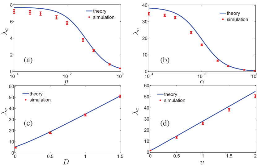
To test the validity of the above expression for the critical coupling, the authors in [67] considered networks following the so-called dense small-world model. In this topology, each node is connected to its $K$ nearest neighbors in both directions in the ring, where $K$ is defined as

$$K=\left\lfloor\frac{\alpha}{2}(N-1)\right\rfloor,\;0\leq\alpha\leq 1.$$ (258)

The variable $\alpha$ tunes the fraction of the total number of nodes $(N-1)/2$ to which each node is coupled. Starting with a ring network and employing this connection strategy leads to a regular network with the degree distribution $P_{\rm{local}}(k)=\delta_{k,2K+1}$. The small-world character of the model is included by the introduction of shortcuts. In contrast to the standard SW model, the shortcuts are not created through the rewiring of already existing edges, but rather by the inclusion of new connections. More specifically, besides the $2K+1$ nearest neighbors that a given node is connected to, a new connection is created between the other $N-K-1$ nodes with probability $p$. In the case $K=0$, the generated structures are ER random networks for $0<p<1$, whereas $p=1$ yields the fully connected graph. The final network has thus the following degree distribution

$$P(k)=\binom{N-2K-1}{k-2K-1}p^{k-2K-1}\left[1-p\right]^{N-k},\textrm{ for }k>2K.$$ (259)

The merit of using the dense small-world world as a substrate to study synchronization of Kuramoto oscillators is the fact that the number of edges linearly scales with the number of nodes, justifying the normalization factor in Eq. 230.

The comparison between the result Eq. 257 and numerical simulations is shown in Fig. 32 as a function of several parameters of the model and considering Gaussian frequency distribution. In particular, in Fig. 32(a) and (b) noise strength $D$ and variance of $g(\omega)$ are kept fixed as the network topology is varied. As it is seen, the denser the networks, the better the agreement with the theoretical prediction, which is expected from the MFA. Noteworthy, the critical coupling $\lambda_{c}$ of the simulated networks is evaluated through FSS analysis, analogously as discussed in Sec. 2, where it is assumed that the order parameter $r$ has the scaling form given by Eq. 13. Interestingly, the same scaling with system’s size observed in the fully connected graph [284, 53] was found in the stochastic Kuramoto model in the dense SW network [67], namely $\beta\approx 1/2$ and $\bar{\nu}\approx 2$. Thus, by calculating the synchronization curves for different network sizes, one is then able to numerically evaluate the critical coupling strength $\lambda_{c}$ (Fig. 32). Moreover, a slight disagreement is also observed for strong standard deviation of the frequency distribution in Fig. 32(d), which is analogous to the discrepancy observed for strongly heterogeneous networks [67].

Sonnenschein et al. [143] also extended the analysis developed in [67] to the case in which the diversity of frequencies is related to the network topology through the joint distribution $P(\omega,k)$. The equations of motion are given by

$$\dot{\theta}_{i}=\omega_{i}+\frac{\lambda}{N^{q}}\sum_{j=1}^{N}A_{ij}\sin\left[\theta_{j}(t)-\theta_{i}(t)\right]+\xi_{i}(t),$$ (260)

where $q$ is a scaling parameter proportional to the number of links in the network. Again, the presence of stochastic forces is accounted for by the terms $\xi_{i}(t)$ which are considered to be sources of Gaussian white noise, satisfying Eq. 231. The natural frequency distribution is assumed to be unimodal and even with standard deviation $\sqrt{\left\langle\omega^{2}_{i}\right\rangle-\left\langle\omega_{i}\right\rangle^{2}}=\upsilon_{n}(k_{i})$, where

$$\upsilon_{n}(k_{i})=\upsilon_{0}\left(\frac{k_{i}}{\left\langle k\right\rangle}\right)^{n},\;n\in\mathbb{R},$$ (261)

with $\upsilon_{0}$ being a constant parameter. The main motivation of the model in Eq. 260 resides in the fact that a direct correlation between frequencies and local connectivity might be hard to be observable in real-world networks [143]. Yet, the process of network formation in real-world systems can in fact yield nodes whose dynamical properties are intrinsically related to the topological structure. This interplay between structure and dynamics is observed, e.g. in neuronal networks, where the neurons connectivity is related to the balance of inhibition and excitation [143].

Assuming the joint probability distribution $P(\omega,k)=g(\omega|k)P(k)$, where the conditional distribution of frequencies $g(\omega|k)$ for a given degree $k$ is given by

$$g_{\rm{gauss}}(\omega|k)=\frac{1}{\sqrt{2\pi\upsilon_{n}(k)}}e^{-\frac{1}{2}\frac{\omega^{2}}{\upsilon_{n}^{2}(k)}},$$ (262)

enables us to show using Eq. 257 that

$$\lambda_{c,{\rm{gauss}}}=2\sqrt{\frac{2}{\pi}}\upsilon_{0}N^{q}\langle k\rangle^{1-n}\left\langle k^{2-n}\textrm{erfc}\left(\frac{D}{\sqrt{2}\upsilon_{n}(k)}\right)\exp\left(\frac{D^{2}}{2\upsilon_{n}(k)^{2}}\right)\right\rangle^{-1}.$$ (263)

In the absence of noise, i.e., $D=0$, the previous equation is reduced to

$$\lambda_{c,{\rm{gauss}}}(D=0)=2\sqrt{\frac{2}{\pi}}\upsilon_{0}N^{q}\frac{\langle k\rangle^{1-n}}{\langle k^{2-n}\rangle}.$$ (264)

It is interesting to note that, if ER networks are considered, for $n=1$ and $2$ the critical coupling coupling $\lambda_{c,{\rm{gauss}}}(D=0)$ has an inverse dependence on the average degree $\left\langle k\right\rangle$. The same result was obtained for linear correlation between frequencies and degrees in [242, 249]. Although, in this model, it is the frequency dispersion that is correlated with local topology, it also leads to similar effects as the ones observed when the frequencies are directly proportional to degrees. For $n>0$, the hubs will potentially have higher frequencies due to the large dispersion, whereas low degree nodes will have narrower distributions. This frequency assignment will contribute to the increase of the critical coupling for the onset of synchronization, since higher couplings are required to entrain the hubs in the mean-field. Finally, for $n<0$, hubs and low degree nodes switch their role, making the network to reach synchronization for lower coupling strengths. Noteworthy, this interplay between the nodes degree and the emergence of a synchronous component was also observed in the model described in Sec. 5 with joint distribution given by Eq. 211.

Furthermore, a curious behavior can be observed if one considers different system-size scaling in the equations of motion. More specifically, changing $N^{q}\rightarrow\mathcal{N}(k)$ in Eq. 260 for two different cases, $\mathcal{N}(k)=\left\langle k\right\rangle$ and $\mathcal{N}(k)=k$, one can show that the critical couplings in the absence of noise ($D=0$) obey

$$\lambda_{c,\left\langle k\right\rangle}=C\upsilon_{0}\frac{\left\langle k\right\rangle^{2-n}}{\left\langle k^{2-n}\right\rangle},\;\lambda_{c,k}=C\upsilon_{0}\frac{\left\langle k\right\rangle^{1-n}}{\left\langle k^{1-n}\right\rangle},$$ (265)

regardless of the frequency distribution adopted, where $\lambda_{c,\left\langle k\right\rangle}$ and $\lambda_{c,k}$ correspond to $\mathcal{N}(k)=\left\langle k\right\rangle$ and $\mathcal{N}(k)=k$, respectively; and $C$ is a proportionality constant, which is different for each frequency distribution. Interestingly, the dependency on the network topology vanishes for some values of $n$. In contrast with the critical coupling in Eq. 264 for scaling $N^{q}$. Note also that the critical couplings related to the scaling terms $\mathcal{N}(k)=\left\langle k\right\rangle$ and $\mathcal{N}(k)=k$ correspond to the shifted version of each other with respect to the correlation power $n$, i.e., $\lambda_{c,\left\langle k\right\rangle}(n)=\lambda_{c,k}(n+1)$.

6.2 Gaussian approximation

The onset of synchronization of the stochastic Kuramoto model in networks can also be derived through a different technique, namely the so-called Gaussian-Approximation [285, 282] (GA). The framework provided by the GA allows a suitable dimension reduction, though it is not exact, in contrast to the OA theory [32], which is, however, not applicable to stochastic systems [282]. Before discussing the stochastic Kuramoto model on networks, let us first briefly introduce the results uncovered through the GA for the fully connected graph.

The equations for the model with identical natural frequencies $\omega_{0}=0$ are

$$\dot{\theta}_{i}=\xi_{i}(t)+\frac{\lambda}{N}\sum_{j=1}^{N}\sin(\theta_{j}-\theta_{i}).$$ (266)

As analysed in the previous section, in the thermodynamic limit $N\rightarrow\infty$, the above system can be described by the density $\rho(\theta,t)$, which satisfies the nonlinear Fokker-Planck equation

$$\frac{\partial\rho}{\partial t}=D\frac{\partial^{2}\rho}{\partial^{2}\theta}-\frac{\partial}{\partial\theta}\left[\lambda r\sin(\psi-\theta)\rho\right],$$ (267)

where $r$ and $\psi$ in the continuum limit are

$$r(t)e^{i\psi(t)}=\int_{0}^{2\pi}d\theta e^{i\theta}\rho(\theta,t).$$ (268)

The Fourier series expansion of $\rho$ yields

$$\rho(\theta,t)=\frac{1}{2\pi}\sum_{n=-\infty}^{+\infty}\hat{\rho}_{n}(t)e^{-in\theta},$$ (269)

where $\rho_{0}=1$ and $\rho_{-n}=\rho_{n}^{*}$, since $\rho(\theta,t)$ is a real function. Using the inverse Fourier transform one obtains

$$\hat{\rho}_{n}(t)=\int_{0}^{2\pi}d\theta\rho(\theta,t)e^{in\theta}\equiv c_{n}(t)+is_{n}(t),$$ (270)

which for $n=1$ yields the order parameter definition in Eq. 268. Substituting Eq. 269 into the nonlinear Fokker-Planck equation (Eq. 267) and grouping the exponential terms leads to the infinite chain of coupled complex-valued equations for the Fourier coefficients given by

$$\frac{\dot{\hat{\rho}}_{n}}{n}=\frac{\lambda}{2}\left(\hat{\rho}_{n-1}\hat{\rho}_{1}-\hat{\rho}_{n+1}\hat{\rho}_{-1}\right)-Dn\hat{\rho}_{n},\;n=1,2,...,\infty.$$ (271)

This equation provides a complete description and, due to the rapidly decay of the coefficients $\hat{\rho}_{n}$ as $n$ increases, it is possible to get relatively accurate results by truncating the system at sufficient large $n$ [282]. However, a thorough bifurcation analysis of the system in Eq. 271 would be difficult or even unfeasible depending on the value of $n$. Thus, in order to find a closure scheme for the infinite set of equations (271), we assume that the phases of the oscillators are distributed according to a Gaussian distribution with mean $\mu(t)$ and variance $\upsilon^{2}(t)$. In this way the coefficients $c_{n}$ and $s_{n}$ in Eq. 270 become [282]

$$c_{n}(t) =\mathrm{e}^{-n^{2}\upsilon^{2}(t)/2}\cos\left[n\mu(t)\right],$$ (272)

$$s_{n}(t) =\mathrm{e}^{-n^{2}\upsilon^{2}(t)/2}\sin\left[n\mu(t)\right],$$

leading to the following Fourier coefficients

$$\left|\hat{\rho}_{n}(t)\right|=e^{-n^{2}\upsilon^{2}(t)/2}.$$ (273)

Changing the variables, one can further show that the mean $\mu$ and the variance $\upsilon^{2}$ evolve according to [282]

$$\dot{\mu}=0\mbox{ and }\dot{\upsilon^{2}}=2D+\lambda\left(\mathrm{e}^{-2\upsilon^{2}}-1\right),$$ (274)

which can be explicitly solved:

$$\upsilon^{2}(t)= \frac{1}{2}\ln\left[\frac{\lambda}{\lambda-2D}+\mathrm{e}^{-2t(\lambda-2D)}\left(\mathrm{e}^{2\upsilon^{2}(0)}-\frac{\lambda}{\lambda-2D}\right)\right],$$ (275)

for $\lambda\neq D$. Note that in the long-time limit $t\rightarrow\infty$ the variance asymptotically converges to

$$\upsilon^{2}(t\rightarrow\infty)=\frac{1}{2}\ln\left(\frac{\lambda}{\lambda-2D}\right).$$ (276)

According to the equation above, for strong couplings $\lambda\rightarrow\infty$, the variance tends to vanish $\upsilon^{2}\rightarrow 0$, characterizing the complete synchronous state. Interestingly, the critical coupling obtained through Eq. 276, $\lambda_{c}=2D$, is the same well-known valued exactly calculated in [279]. The time evolution of the order parameter $r(t)$ can also be derived thanks to the closure scheme provided by the GA. More specifically, all coefficients $c_{n}$ and $s_{n}$ depend on $c_{1}$ and $s_{1}$. Therefore, using Eq. 271 the following system of equations is obtained [282, 285]

$$\dot{c}_{1} =-Dc_{1}+\frac{\lambda c_{1}}{2}\left\{1-\left[\left(c_{1}\right)^{2}+\left(s_{1}\right)^{2}\right]^{2}\right\},$$ (277)

$$\dot{s}_{1} =-Ds_{1}+\frac{\lambda s_{1}}{2}\left\{1-\left[\left(c_{1}\right)^{2}+\left(s_{1}\right)^{2}\right]^{2}\right\}.$$

Noting that $c_{1}=r$ and $s_{1}=0$, one derives

$$\dot{r}=\frac{r}{2}\left[\lambda\left(1-r^{4}\right)-2D\right],$$ (278)

for which in the stationary regime $\dot{r}=0$ and neglecting the term $r^{4}$ near the onset of synchronization also leads to the critical coupling $\lambda_{c}=2D$.

The generalization to the network case can be done straightforwardly, although the dimensionality reduction is not as drastic as in the fully connected graph. The population of oscillators is described by the phase distribution $\rho(\theta,t|k)$, i.e., the dependency on a given degree $k$ is introduced. With this definition, the coherence inside each population of oscillators with the same degree $k$ is calculated by

$$r_{k}(t)\mathrm{e}^{i\psi_{k}(t)}=\int_{0}^{2\pi}d\theta^{\prime}\ \mathrm{e}^{i\theta^{\prime}}\ \mathcal{\rho}\left(\theta^{\prime},t|k\right).$$ (279)

The total order parameter is then given by

$$r(t)\mathrm{e}^{i\psi(t)}=\frac{1}{\langle k\rangle}\int dk^{\prime}P(k^{\prime})k^{\prime}r_{k^{\prime}}(t)\mathrm{e}^{i\psi_{k^{\prime}}(t)},$$ (280)

Using the GA one is able to show that the closure scheme yields

$$\dot{r}_{k} = \frac{1-\left(r_{k}\right)^{4}}{2N\left\langle k\right\rangle}\lambda k\left\langle k^{\prime}r_{k^{\prime}}\cos(\psi_{k^{\prime}}-\psi_{k})\right\rangle_{k}-r_{k}D$$

$$\dot{\psi}{}_{k} = \frac{\left(r_{k}\right)^{-1}+\left(r_{k}\right)^{3}}{2N\left\langle k\right\rangle}\lambda k\left\langle k^{\prime}r_{k^{\prime}}\sin(\psi_{k^{\prime}}-\psi_{k})\right\rangle_{k},$$

where $\langle...\rangle_{k}=\int dk...P(k)$ is the average over the degree distribution $P(k)$. Note that the populations of different degrees are coupled through the averages $\langle...\rangle_{k}$. Assuming $\psi_{k}=0$ $\forall k$, the evolution of the total order parameter is given by

$$\dot{r}^{g}=\frac{\lambda}{2N\langle k\rangle}\left\langle k^{\prime 2}\left[1-\left(r_{k^{\prime}}^{g}\right)^{4}\right]\right\rangle_{k}r^{g}-Dr^{g}.$$ (281)

In the stationary state, neglecting the terms $r_{k^{\prime}}^{4}$ leads to the critical coupling

$$\lambda_{c}=2DN\frac{\left\langle k\right\rangle}{\left\langle k^{2}\right\rangle}$$ (282)

which is the same result as obtained with Eq. 257 for identical oscillators.

The GA technique was also employed in the analysis of heterogeneous networks made up of stochastic Shinomoto-Kuramoto active rotator oscillators [86]. The model proposed in [81] consists of a slight modification of the original Kuramoto model that encompasses the properties of excitable systems. Excitable behavior and collective oscillations are found in many different systems, including physical, chemical and biological ones, with a wide range of applications [286]. Excitability in a given system is characterized by the presence of a stable equilibrium of its units, which can be replaced by a non-monotonic behavior when the system is subjected to sufficiently strong perturbations.

The equations of the networks considered in [86] are given by

$$\dot{\theta}_{i}(t)=1-a\sin\left(\theta_{i}(t)\right)+\frac{\lambda}{N}\sum_{j=1}^{N}A_{ij}\sin\left(\theta_{j}(t)-\theta_{i}(t)\right)+\xi_{i}(t),$$ (283)

where $a$ is the excitability threshold of the model. For a system with only one oscillator without the presence of noise, $\dot{\theta}_{i}=1-a\sin\theta_{i}$, an excitable behavior is achieved for $|a|>1$ and the stationary solution is $\theta_{i}=\arcsin\left(a^{-1}\right)$. On the other hand, if $|a|<1$, the system is in an oscillatory regime with frequency $\sqrt{1-a^{2}}$. Noteworthy, contrary to the standard Kuramoto model, phase $\theta_{i}$ does not rotate uniformly, the slowest and fastest points are near $\phi=\pi/2$ and $3\pi/2$, respectively [81, 287, 286, 86]. As before, the network is described by the one-oscillator probability density $\rho(\theta,t|k)$, where $\rho(\theta,t|k)d\theta$ gives the fraction of oscillators with phase between $\theta$ and $\theta+d\theta$ at time $t$ for a given degree $k$. The Fourier expansion of $\rho$ leads to

$$\rho(\theta,t|k)=\frac{1}{2\pi}\sum_{n=-\infty}^{\infty}\hat{\rho}_{n}(t|k)e^{-in\theta},$$ (284)

where the coefficients, which now are also defined for a given degree $k$, can be written as

$$\hat{\rho}_{n}(t|k)=c_{n}(t|k)+is_{n}(t|k),\;n=1,2,...,\infty.$$ (285)

Substituting Eq. 284 in the corresponding nonlinear Fokker-Planck, one can show that for every $k$ the following infinite chain of coupled complex-valued equations determines the evolution of the coefficients $\rho_{n}(t|k)$:

$$\frac{\dot{\hat{\rho}}_{n}(t|k)}{n}= \frac{\tilde{\lambda}k}{2\langle k\rangle}\left(\hat{\rho}_{n-1}(t|k)\left\langle\hat{\rho}_{1}(t|k^{\prime})k^{\prime}\right\rangle_{k}-\hat{\rho}_{n+1}(t|k)\left\langle\hat{\rho}_{-1}(t|k^{\prime})k^{\prime}\right\rangle_{k}\right)$$ (286)

$$+\frac{a}{2}\left(\hat{\rho}_{n-1}(t|k)-\hat{\rho}_{n+1}(t|k)\right)-(Dn-i)\hat{\rho}_{n}(t|k).$$

Similarly as before, it is assumed that the phases of each subpopulation formed by nodes with the same degree $k$ follow a Gaussian distribution with mean $\mu_{k}(t)$ and variance $\upsilon^{2}_{k}(t)$. Thus, in the thermodynamic limit $N\rightarrow\infty$ one can show that in the GA the coefficients $c_{n}$ and $s_{n}$ in Eq. 285 are given by

$$c_{n}(t|k)=\mathrm{e}^{-n^{2}\upsilon_{k}^{2}(t)/2}\cos\left(n\mu_{k}(t)\right),\ \ s_{n}(t|k)=\mathrm{e}^{-n^{2}\upsilon_{k}^{2}(t)/2}\sin\left(n\mu_{k}(t)\right).$$ (287)

Applying the closure, scheme the reduced system of equations for the variables $\mu_{k}(t)$ and $\upsilon_{k}(t)$ is obtained [86]

$$\dot{\mu}_{k}= 1-\mathrm{e}^{-\upsilon_{k}^{2}/2}\cosh\upsilon_{k}^{2}$$ (288)

$$\times\left[a\sin\mu_{k}-\frac{\tilde{\lambda}k}{\langle k\rangle}\left(\langle k^{\prime}\mathrm{e}^{-\upsilon_{k^{\prime}}^{2}/2}\sin\mu_{k^{\prime}}\rangle_{k}\cos\mu_{k}-\langle{k^{\prime}}\mathrm{e}^{-\upsilon_{k^{\prime}}^{2}/2}\cos\mu_{k^{\prime}}\rangle_{k}\sin\mu_{k}\right)\right],$$

$$\dot{\upsilon}_{k}^{2}= 2D-2\mathrm{e}^{-\upsilon_{k}^{2}/2}\sinh\upsilon_{k}^{2}$$

$$\times\left[a\cos\mu_{k}+\frac{\tilde{\lambda}k}{\langle k\rangle}\left(\langle k^{\prime}\mathrm{e}^{-\upsilon_{k^{\prime}}^{2}/2}\sin\mu_{k^{\prime}}\rangle_{k}\sin\mu_{k}+\langle{k^{\prime}}\mathrm{e}^{-\upsilon_{k^{\prime}}^{2}/2}\cos\mu_{k^{\prime}}\rangle_{k}\cos\mu_{k}\right)\right].$$

Again, the dimensionality reduction in the network case is not as severe as for the dynamics in the fully connected graph. The number of coupled equations one is left with is equal to twice the number of different degrees in the network, if the oscillators are identical. Generalizations for the Ott-Antonsen also share this property [288, 289, 96], in fact some approaches yield reduced systems with similar size as the original ones [288]. Nevertheless, the impact of network heterogeneity can be comprehensively analysed for some special topologies, which can then be used as insights to the understanding of the dynamics of more sophisticated structures. In particular, for regular networks, Eqs. 288 are reduced to

$$\dot{\mu}_{k}=1-a\mathrm{e}^{-\upsilon_{k}^{2}/2}\cosh\upsilon_{k}^{2}\sin\mu_{k},\quad\dot{\upsilon}_{k}^{2}=2D-2\mathrm{e}^{-\upsilon_{k}^{2}/2}\sinh\upsilon_{k}^{2}\left[a\cos\mu_{k}+\tilde{\lambda}k\mathrm{e}^{-\upsilon_{k}^{2}/2}\right].$$ (289)

Figure 33: Critical noise strength $D_{c}$ as a function of connectivity fraction $\alpha$ of regular networks for excitation threshold (a) $a<1$ and (b) $a>1$ determined through numerical bifurcation analysis of the reduced system in Eq. 290. Panels (c) and (d) show $D_{c}$ as a function of $\textrm{Var}(\alpha)/\textrm{VarMax}$ of the reduced system in Eq. 291 for binary networks considering $a<1$ and $a>1$, respectively; where $\left\langle\alpha\right\rangle=0.4$ and $\textrm{Var}(\alpha)/\textrm{VarMax}=0.25$. In all panels coupling strength is set to $\lambda=1$ and SN indicate saddle-node bifuracations. Adapted with permission from Springer Science+Business Media [86].

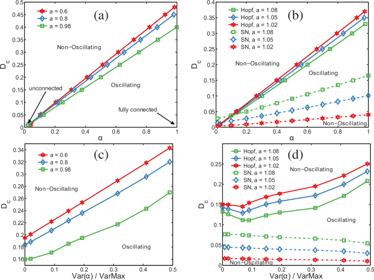
As shown in [86], system (289) has exactly the same bifurcation diagram on the plane $a-D$ as the correspondent system for the fully connected graph, the equations only differ by a rescaling of the effective mean-field $\lambda\rightarrow k\lambda/N$. For sufficient large values of noise intensity $D$, changes in the excitability threshold $a$ have no effect on the system’s stability. On the order hand, for moderate values of $D$, the oscillators can transit through Hopf and saddle-node bifurcation between regimes of synchronous and asynchronous firing and coherent oscillations with the absence of excitability [86, 285]. Although the regular network exhibits a perfectly homogeneous topology, it still serves as a special model to analyze how the density of connections impacts on the such transitions. Let $D_{c}$ denote the bifurcation value of the noise strength - or also called as critical noise strength -, Fig. 33(a) and (b) show its dependence on the variable $\alpha=k/N$, which quantifies the density of the regular network, for different values of $a$. The regions “Non-oscillating” and “Oscillating” denote the asynchronous and synchronous regimes, respectively. Moreover, the state in which the active rotators fire coherently and the state in which they are synchronized without firing are treated indiscriminately as the “Oscillating” state in Fig. 33 in order to purely investigate the impact of the network topology on the overall dynamics. As it is seen, the bifurcation point $D_{c}$ is almost linearly related with the parameter $\alpha$, in a way that the variation of network density does not lead to novel phenomena in the network dynamics; the effective mean-field is only rescaled by such a modification in the topology [86]. Furthermore, for $a<1$ (Fig. 33( (a)) only Hopf bifurcations are observed, whereas for $a>1$ (Fig. 33 (b)) saddle-node bifurcations also emerge [86].

Topological heterogeneity can be included by considering a network with only two different degrees. The random binary network provides the simplest heterogeneous degree distribution, which is characterized by the degrees $k_{1}$ and $k_{2}$ (and the respective densities $\alpha_{1}=k_{1}/N$ and $\alpha_{2}=k_{2}/N$) given by

$$P(k)=p\delta_{k,k_{1}}+(1-p)\delta_{k,k_{2}}$$ (290)

By fixing the average density $\left\langle\alpha\right\rangle$ (or equivalently the average degree $\left\langle k\right\rangle$) and varying the $\alpha_{1}$ and $\alpha_{2}$, it is possible to tune $\textrm{Var}(\alpha)$ up to the upper bound $\textrm{VarMax}=0.25$ so that the bifurcation points can be analysed as a function of the disparity of connections between the subpopulations. Using the degree distribution in Eq. 290, the reduced system in Eq. 288 can be rewritten for the binary network case as

$$\dot{\mu}_{1}= 1-\mathrm{e}^{-\upsilon_{1}^{2}/2}\cosh(\upsilon_{1}^{2})\left[a\sin(\mu_{1})+\frac{\lambda\alpha_{1}\alpha_{2}(1-p)}{p\alpha_{1}+(1-p)\alpha_{2}}\sin(\mu_{1}-\mu_{2})\mathrm{e}^{-\upsilon_{2}^{2}/2}\right]$$ (291)

$$\dot{\upsilon}_{1}^{2}= 2D-2\mathrm{e}^{-\upsilon_{1}^{2}/2}\sinh(\upsilon_{1}^{2})$$

$$\times\left[a\cos(\mu_{1})+\frac{\lambda\alpha_{1}}{p\alpha_{1}+(1-p)\alpha_{2}}\left(\alpha_{1}p\mathrm{e}^{-\upsilon_{1}^{2}/2}+\alpha_{2}(1-p)\mathrm{e}^{-\upsilon_{2}^{2}/2}\cos(\mu_{1}-\mu_{2})\right)\right]$$

$$\dot{\mu}_{2}= 1-\mathrm{e}^{-\upsilon_{2}^{2}/2}\cosh(\upsilon_{2}^{2})\left[a\sin(\mu_{2})+\frac{\lambda\alpha_{1}\alpha_{2}p}{p\alpha_{1}+(1-p)\alpha_{2}}\sin(\mu_{2}-\mu_{1})\mathrm{e}^{-\upsilon_{1}^{2}/2}\right]$$

$$\dot{\upsilon}_{2}^{2}= 2D-2\mathrm{e}^{-\upsilon_{2}^{2}/2}\sinh(\upsilon_{2}^{2})$$

$$\times\left[a\cos(\mu_{2})+\frac{\lambda\alpha_{2}}{p\alpha_{1}+(1-p)\alpha_{2}}\left(\alpha_{2}(1-p)\mathrm{e}^{-\upsilon_{2}^{2}/2}+\alpha_{1}p\mathrm{e}^{-\upsilon_{1}^{2}/2}\cos(\mu_{2}-\mu_{1})\right)\right],$$

where $\alpha_{1}=k_{1}/N$ and $\alpha_{2}=k_{2}/N$ are the connectivity fraction of each subpopulation. Fig. 33 (c) and (d) show the dependence of the critical noise strength $D_{c}$ on the variance $\textrm{Var}(\alpha)$. For $a<1$, $D_{c}$ exhibits similar dependence on $\textrm{Var}(\alpha)/\textrm{VarMax}$ as on $\alpha$ in regular networks, i.e., almost linear growing with Hopf bifurcations connecting the states. However, for $a>1$, the critical noise strength $D_{c}$ associated to the saddle-node bifurcation decreases as the degree distribution becomes more heterogeneous, enlarging the oscillating region. Another interesting behavior is that the Hopf bifurcation lines are no longer monotonic as a function of $\textrm{Var}(\alpha)$. As seen in Fig.  33(d), $D_{c}$ reaches minimal values for slight heterogeneous networks, a phenomenon induced by the presence of a small fraction of highly connected nodes [86].

The active rotator model in the absence of noise in uncorrelated networks was studied in [290] in the presence of attractive and repulsive couplings strengths. The authors verified that the network heterogeneity, along with the repulsive couplings, induces global firing in the ensemble, an effect that is akin to the collective firings promoted by noise and quenched disorder in globally coupled oscillators [85]. Strangely, despite its rich dynamics, the Shinomoto-Kuramoto model has been rarely tackled in heterogeneous networks in a way that many aspects of the influence of the connectivity pattern on the population coherence and excitability remain to be investigated. For instance, Sonnenschein et al.  [87] recently investigated the Shinomoto-Kuramoto model in the fully connected graph where the natural frequencies and individual coupling strengths are correlated. More specifically, a system made up of two equally sized populations of oscillators, each one characterized by the pairs $(\omega_{1},\lambda_{1})$ and $(\omega_{2},\lambda_{2})$, was studied. Interestingly, it was found that global excitability is only reached when the excitable units have smaller coupling strengths than the self-oscillatory ones  [87]. This particular frequency-coupling correlation naturally motivates further generalizations of the model, such as in modular and mutilayer networks  [17, 18], in which other interesting dynamical patterns can possibly arise by the introduction of network connectivity.

Besides the theoretical approaches described above, other aspects of the dynamics of the stochastic Kuramoto model were numerically addressed [291, 292, 283, 293, 294, 295]. In particular, Traxl et al. [283] developed a numerical framework and systematically analyzed the influence of noise and coupling strength on the maximum degree of synchronization of several networks; including fully connected, random, modular and real topologies. For all the cases considered, the authors reported that the maximum degree of synchronization is suitably fitted by a 2-dimensional sigmoidal function linearly related with the noise and coupling strength [283].

7 Second-order Kuramoto model

The first-order Kuramoto model is analytically tractable and exhibits a large variety of synchronization phenomena in different contexts (see Sec. 2). However, it approaches too fast the partial synchronized state compared to experimental observations and an infinite coupling strength is required to achieve perfect synchronization [296]. The model with frequency adaptation, where both phase and frequency evolve in time and having synchronization slowed down by inertia, can solve such problems. Therefore, the second-order Kuramoto model (or the Kuramoto model with inertia) has been extensively investigated. The model with inertia was firstly explored in biological contexts. In the early 90’s, motivated by the fact that certain species of fireflies, like Pteroptyx malaccae, are able to achieve perfect synchronization even for a stimulating frequency different from their intrinsic frequency, Ermentrout [209] proposed a model with frequency adaptation which has the ability to mimic such a perfect synchrony between coupled oscillators. Strogatz [297] and later Trees et al. [298] showed that the same model can be obtained from capacitively shunted junction equations to study synchronization in disordered arrays of Josephson junctions. Moreover Filatrella et al. [299] derived this model from the classical swing equation to study synchronization in power grids (see Sec. 9).

In this section, we will explain the second-order Kuramoto model from different points of view. From a methodological standpoint, as the focus of this section, we first explain the collective behavior of a set of coupled Kuramoto model with inertia using a mean-field analysis [300, 301] and substantially extend the theory to the second-order Kuramoto model with frequency-degree correlation [244]. Subsequently, we quantify the stability of networks of coupled oscillators in terms of the basin of attraction of the synchronized state against large perturbations using the new concept of basin stability ($\mathcal{BS}$) [302]. In particular, we focus on the interplay between $\mathcal{BS}$ and underlying structures.

7.1 Second-order Kuramoto model in complex networks

The second-order Kuramoto model consists of an ensemble of coupled phase oscillators, $\theta_{i}$ for $i=1,\dots,N$, whose dynamics are governed by

$$\ddot{\theta}_{i}=-\alpha\dot{\theta}_{i}+\omega_{i}+\lambda\sum\limits^{N}_{j=1}A_{ij}\sin{(\theta_{j}-\theta_{i})},$$ (292)

where $\alpha$ is the dissipation parameter. If the left part of this equation is set to zero, we recover the first-order Kuramoto model. In comparison to the first-order Kuramoto model, the second-order mode exhibits a region of bistability in the bifurcation diagram, which will be shown below.

7.1.1 Illustration

In order to get insights into the fundamental dynamics of Eq. 292, let us consider the one-node model, where one node is connected to a grid and whose dynamics follows

$$\ddot{\theta}=-\alpha\dot{\theta}+\omega+\lambda\sin{(\theta_{L}-\theta)},$$ (293)

where $\theta_{L}$ is the phase of the large system. The grid is regarded to be infinite in the sense that its state can not be affected by the node’s dynamics. Hence, here we set $\theta_{L}\equiv 0$, without loss of generality. Such a model also depicts the governing dynamics of the driven pendulum [297], Josephson junctions [297] and the one-machine infinite bus system of a generator in a power-grid [303]. The corresponding governing dynamics can also depict a two-node model with the same bifurcation diagram [304].

We can define the energy function $E(\nu,\omega)$ for model (293) as [303]

$$E(\theta,\nu)=E_{k}(\nu)+E_{p}(\theta),$$ (294)

where $\nu\equiv\dot{\theta}$ and the kinetic and potential energy are given by$E_{k}(\nu)=\frac{\nu^{2}}{2}$ and $E_{p}(\theta)=-\omega\theta-\lambda\cos{(\theta)}$, respectively. In the absence of damping and external driving, i.e. $\alpha=0$ and $\omega=0$, by introducing a dimensionless time $\tau=\sqrt{\lambda}t$, Eq. (293) becomes

$$\frac{d^{2}\theta}{d\tau^{2}}=-\sin{\theta}.$$ (295)

Such system has two fixed points within the range $[0,2\pi)$. One fixed point $(\theta^{*},\nu^{*})=(\pi,0)$ is a saddle. The other one is located at $(\theta^{*},\nu^{*})=(0,0)$. The origin is a nonlinear center, as the system is reversible and conservative with the energy function $E(\theta,\nu)=\nu^{2}/2-\cos(\theta)=\mathrm{constant}$. A local minimal energy is located at the fixed point with $E(0,0)=-1$ [297]. Small orbits around the center are small oscillations, called librations. The obits grow with an increase in $E$ until $E=1$ along with the heteroclinic trajectories linking the saddles. With further increases in $E$, i.e. $E>1$, the system starts oscillating periodically over or below the heteroclinic trajectories [297].

Furthermore, via including a linear damping to this system, i.e. $\alpha>0$ but with $\omega=0$, the system therein has one stable fixed point at $(\theta^{*},\nu^{*})=(0,0)$ and one saddle $(\theta^{*},\nu^{*})=(\pi,0)$ [297]. With small damping, vibrations start converging to the stable fixed point. The energy decreases monotonically along the trajectories with the rate $\frac{dE(\theta,\nu)}{dt}=\frac{d(\nu^{2}/2-\lambda\cos(\theta))}{dt}=-\alpha\nu^{2}$, except for the fixed points with $\nu^{*}=0$.

Finally, the third case is the complete original system (293) with damping as well as external driving, i.e. $\alpha>0$ and $\omega>0$. For convenience, one could either set $\lambda=1$ or introduce a dimensionless time $\tau=\sqrt{\lambda}t$. The bifurcation diagram is shown in Fig. 34. For $\omega>1$, all rotations converge to a unique and stable limit cycle and no fixed points are available in the region of the stable limit cycle. For $\omega<1$, two fixed points comprise a saddle and a sink, satisfying $\nu^{*}=0$ and $\sin(\theta^{*})=\omega$. The linear stability of the fixed points is determined by the Jacobian matrix

$$J=\left(\begin{array}[]{cc}0&1\\ -\cos(\theta^{*})&-\alpha\end{array}\right)$$

with two eigenvalues

$$\sigma_{1,2}=\frac{-\alpha\pm\sqrt{\alpha^{2}-4\cos(\theta^{*})}}{2}.$$ (296)

The fixed point with $\cos(\theta^{*})=-\sqrt{1-\omega^{2}}$ with $\sigma_{1}>0$ and $\sigma_{2}<0$ is a saddle. The other fixed point with $\cos(\theta^{*})=\sqrt{1-\omega^{2}}$ is stable due to its real part of both eigenvalues $\mathrm{Re}(\sigma_{1,2})<0$. Moreover, it is a stable node for $\alpha^{2}-4\sqrt{1-\omega^{2}}>0$ and a stable spiral, otherwise (separated by the blue dashed line in Fig. 34).

There are three types of bifurcations in the bifurcation diagram in Fig. 34. For small $\alpha$ and suppose that we start from $\omega>1$, the system rotates periodically. We slowly decrease $\omega$ and, at some critical value $\omega_{c}<1$, rotations merge with the saddle and are destroyed in a homoclinic bifurcation. Its critical value is determined by

$$\omega_{c}=\frac{4\alpha}{\pi},$$ (297)

as $\alpha\rightarrow 0$ based on the Melnikov’s analysis [297]. This bifurcation line separates the region of bistability and the region of globally stable fixed point. Noteworthy, this result can also be obtained by employing Lyapunov’s second method [305]. For large $\alpha$, we slowly decrease $\omega$ from $\omega>1$. The rotations are destroyed by an infinite-period bifurcation and fixed points appear. Suppose that we start from a stable fixed point for small $\alpha$ and slowly increase $\omega$, two fixed points collide and annihilate each other in a saddle-node bifurcation with $\omega_{c}=1$.

Figure 34: Bifurcation diagram of the one-node model (293). In the grey region only the stable limit cycle exists. The red region indicates the globally stable fixed point. In the region of bistability, stable fixed point and stable limit cycle coexist. The blue dashed line is plotted at $\alpha^{2}=4\sqrt{1-\omega^{2}}$. Here we set $\lambda=1$.

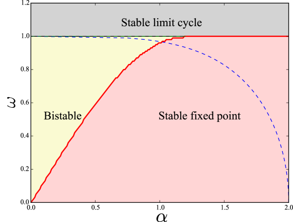
The node can either converge to a fixed point or oscillate periodically in the region of bistability. Menck et al. [302] proposed a way to approximate the curve of the stable cycle. For $\lambda=0$, the model (293) has one stable limit cycle with frequency $\nu(t)=\omega/\alpha$ and phase $\theta(t)=\nu(t)t+\theta(0)$. For large $\lambda$, a similar solution is still fulfilled with the average frequency $\left\langle\nu\right\rangle=\int\limits^{T}_{t=0}\nu(t)dt/T\approx\omega/\alpha$ and $\theta(t)\approx\left\langle\nu\right\rangle t+\theta(0)$, where $T$ is a long integrating period. To derive an expression of the instant frequency, the frequency $\nu(t)$ is assumed to fluctuate around the average frequency $\left\langle\nu\right\rangle$ as $\nu(t)=\left\langle\nu\right\rangle+f(t)$, where $f(t)$ remains to be solved. Inserting this into Eq. (293) yields

$$\dot{f}=-\alpha f-\lambda\sin(\left\langle\nu\right\rangle t+\theta(0)),$$ (298)

which has one special solution as follows

$$f(t)=-\frac{\alpha\lambda}{\left\langle\nu\right\rangle^{2}+\alpha^{2}}\left(\sin\left(\left\langle\nu\right\rangle t+\theta(0)\right)-\frac{\left\langle\nu\right\rangle}{\alpha}\cos\left(\left\langle\nu\right\rangle t+\theta(0)\right)\right).$$ (299)

For $\left\langle\nu\right\rangle\gg\alpha$ and via inserting $\left\langle\nu\right\rangle\approx\omega/\alpha$ into Eq. (299), the instant frequency therein is approximated by [302]

$$\nu(t)\approx\omega/\alpha+\frac{\alpha\lambda}{\omega}\cos(\omega t/\alpha+\theta(0)).$$ (300)

Equation (300) is in good agreement with numerical results [302, 306]. Integrating Eq. (300) yields [302]

$$\theta(t)\approx\omega t/\alpha+\frac{\alpha^{2}\lambda}{\omega^{2}}\sin{(\omega t/\alpha+\theta(0))+\theta(0)}.$$ (301)

If $\omega^{2}\gg\alpha^{2}\lambda$, $\theta(t)\approx\omega t/\alpha+\theta(0)$ which is consistent with the previous assumption.

7.1.2 Mean-field theory without noise

In the previous subsection, we explain the basic dynamics of the one-node model, in this and next subsections, we will explain networked oscillators without and with noise, respectively.

Tanaka et al. [301, 300] were the first to analyze the collective behavior of a set of coupled Kuramoto model with finite (large) inertia. Due to the finite inertia, the system exhibits a first-order phase transition, with discontinuous jumps and hysteresis, different from the second-order transition obtained from the Kuramoto model without inertia. In particular, the mean-field framework is provided for investigating the hysteretic behavior in the large network size and validated theoretical results with a uniform, bounded intrinsic frequency distribution. To compare with the case of without inertia, the following general form of the second-order Kuramoto model was considered [301, 300]

$$m\ddot{\theta}_{i}=-\alpha\dot{\theta}_{i}+\omega_{i}+\frac{\lambda}{N}\sum\limits^{N}_{j=1}\sin{(\theta_{j}-\theta_{i})},$$ (302)

where $m\ddot{\theta}_{i}$ denotes the inertia of the $i$-th oscillator. After a suitable coordinate transformation via replacing the coupling term by the mean-field quantities $(R,\psi)$ and assuming $\alpha=1$, Eq. (302) is rewritten as

$$m\ddot{\theta}_{i}=-\dot{\theta}_{i}+\omega_{i}+\lambda R\sin{(\psi-\theta_{i})}.$$ (303)

In the stationary state, the set of oscillators is split into one subgroup of oscillators locked to the mean phase and the other subgroup of drifting oscillators whirling over (or below depending on the sign of $\omega$) the locked subgroup. Therefore, the overall phase coherence $R$ sums two certain coherence $R_{\mathrm{lock}}$ and $R_{\mathrm{drift}}$, contributed by these two subgroups, respectively, i.e.,

$$R=R_{\mathrm{lock}}+R_{\mathrm{drift}}.$$ (304)

To detect multistability of the system, two kinds of simulations are considered: increasing (I) and decreasing (D) adiabatically the coupling strength $\lambda$ [301, 300], respectively. Note that the analytical process is similar to that of the first-order Kuramoto model (see Sec. 2) but with different synchronization conditions. (I) When $\lambda$ increases from a small value, the phase coherence $R^{\mathrm{I}}$ persists around a small fluctuation due to effects of network sizes until a critical coupling strength, denoted by $\lambda^{\mathrm{I}}_{c}$. Above $\lambda^{\mathrm{I}}_{c}$, the system jumps to a weakly synchronized state. $R^{\rm{I}}$ increases with further increases in $\lambda$ and then saturates to a constant value for sufficiently large coupling strengths. (D) When $\lambda$ decreases from a sufficiently large value, the system is initially in the strongly synchronized state and $R^{\mathrm{D}}$ remains nearly constant until a critical coupling strength, denoted by $\lambda^{\mathrm{D}}_{c}$. Beyond this threshold, the system jumps back to the incoherent state. Hysteretic behaviors therein are observed. Two critical coupling strengths $\lambda^{\mathrm{I}}_{c}$ and $\lambda^{\mathrm{D}}_{c}$ are almost the same for small $m$ (e.g. $m=0.95$) but its difference enlarges for large $m$ (e.g. $m=2.0$ or $6.0$) [300]. Noteworthy, $\lambda^{\mathrm{D}}_{c}$ is the same as that of the first-order Kuramoto model [301]. Different dynamical regimes are observed [300, 301], including the incoherent state (IS), the weakly synchronized state (WSS), the strongly synchronized state (SSS), a transition state from WSS to SSS and vice-versa.

In case ($\mathrm{I}$), all oscillators initially drift around its own natural frequency $\omega_{i}$. With increasing $\lambda$, oscillators with a small natural frequency below the threshold $\omega_{\mathrm{I}}$, i.e. $|\omega_{i}|<\omega_{\mathrm{I}}$, start being attracted to the locked group. With further increases in $\lambda$, $\omega_{\mathrm{I}}$ enlarges, oscillators with a large natural frequency become synchronized and the phase coherence $R^{\mathrm{I}}$ increases. For sufficiently large coupling, $\omega_{\mathrm{I}}$ exhibits plateaus and $R^{\mathrm{I}}\approx 1$. If the inertia is rather small, i.e. $\frac{1}{\sqrt{m\lambda R^{\mathrm{I}}}}\ll 1$, the homoclinic bifurcation is tangent to the line (297). Using Melnikov’s method one is able to obtain $\omega_{\mathrm{I}}=\frac{4}{\pi}\sqrt{\frac{\lambda R^{\mathrm{I}}}{m}}$ [301]. During this process, a secondary synchronization of drifting oscillators is observed for larger $m$. This phenomenon was confirmed in [307], where the synchronized motions were validated by comparing the evolution of the instantaneous frequency $\nu_{i}(t)=\dot{\theta}_{i}$ of the secondary synchronized oscillators in random networks and also in the Italian high-voltage power grid.

In case ($\mathrm{D}$), initially almost all oscillators are locked to the mean phase $\psi$ if the initial coupling strength $\lambda$ is large enough, and $R^{\mathrm{D}}\approx 1$. With decreasing $\lambda$ further, locked oscillators are desynchronized and start whirling when their natural frequency exceeds the threshold $\omega_{\rm{D}}$, i.e. $|\omega_{i}|>\omega_{\rm{D}}=\lambda R^{\mathrm{D}}$, where a saddle node bifurcation occurs. Therefore, given the synchronization boundary $\omega_{\mathrm{I}}$ and $\omega_{D}$, the contribution to the locked coherence follows [300, 301, 307]

$$R^{\mathrm{I,D}}_{\mathrm{lock}}=\lambda R^{\mathrm{I,D}}\int^{\theta_{{\mathrm{I}},{\mathrm{D}}}}_{-\theta_{\mathrm{I,D}}}\cos^{2}{\theta}g(\lambda R^{\mathrm{I,D}}\sin\theta)d\theta,$$ (305)

where $\theta_{\mathrm{I}}=\sin^{-1}(\omega_{\mathrm{I}}/(\lambda R^{\mathrm{I}}))$ and $\theta_{\mathrm{D}}=\sin^{-1}(\omega_{\mathrm{D}}/(\lambda R^{\mathrm{D}}))$.

The phase coherence from drifting oscillators takes the same form as in the first-order Kuramoto model [4] and is given by [300, 301, 307]

$$R^{\mathrm{I,D}}_{\mathrm{drift}}=\int_{|\omega|>\omega_{\mathrm{I,D}}}\int e^{i\theta}\rho_{\mathrm{drift}}(\theta,\omega)g(\omega)d\theta d\omega,$$ (306)

where $\rho_{\mathrm{drift}}$ is the density of the drifting oscillators with the phase $\theta$ and frequency $\omega$. $\rho_{\mathrm{drift}}(\theta,\omega)$ is proportional to $|\nu|^{-1}$, i.e. $\rho_{\mathrm{drift}}(\theta,\omega)=\frac{\hat{\omega}}{2\pi}|\nu|^{-1}$, where $\hat{\omega}$ is the frequency of the periodic solution of $\theta$ [301]. Expanding the cosine function in terms of the Bessel functions and applying the Poicare-Lindstead method [301], Eq. (306) can be simplified as

$$R^{\mathrm{I,D}}_{\mathrm{drift}}=\int_{|\omega|>\omega_{\mathrm{I,D}}}\int^{\hat{T}}_{0}\cos(\theta(t,\omega))g(\omega)dtd\omega,$$ (307)

where $\hat{T}=\frac{2\pi}{\hat{\omega}}$ is the period of the running periodic solution of $\theta$. This theoretical framework can be extended to a general distribution of $g(\omega)$ with extended tails to solve the self-consistent equations of $R$ analytically [300].

Now, consider the same dynamics (302) with natural frequencies distributed according to the Gaussian distribution $g(\omega)=\frac{1}{\sqrt{2\pi}}e^{-\omega^{2}/2}$ [307]. To numerically investigate the hysteretic loop of the locked natural frequency threshold as a function of $\lambda$ within the range $[\lambda^{\mathrm{D}}_{c},\lambda^{\mathrm{I}}_{c}]$, one can record the maximal locked natural frequency $\omega_{\rm{I}}$ ($\omega_{\rm{D}}$) with respect to the increasing (decreasing) coupling strength $\lambda$ in steps $\delta\lambda$ in order to uncover the hysteresis. Note that the results are independent of the step size [307]. Recalling that within the interval $[\lambda^{\mathrm{D}}_{c},\lambda^{\mathrm{I}}_{c}]$, incoherent and strongly synchronized states coexist [300, 301]. Such results can also be validated via perturbing incoherent states [307]. In particular, initially the system is in the asynchronous state. At each $\lambda$, all the oscillators with $|\omega_{i}|<\omega_{S}$ are locked to the mean phase, and then the mean phase coherence $r$ is recorded after a long transient time, where $\omega_{S}$ is an artificial threshold. To identify the interval $[\lambda^{\mathrm{D}}_{c},\lambda^{\mathrm{I}}_{c}]$, at each $\lambda$, via increasing $\omega_{S}$ from small to high values, the lowest value of $\omega_{S}$ is taken as minimal $\omega_{S}$ when a coherent state is observable, otherwise $\omega_{S}=0$ it is set [307]. Using this process, the critical coupling interval can also be reproduced (Fig. 35). These results give insights on the probability of the system retaining to the coherent or incoherent states [34, 302].

Figure 35: Minimal $\omega_{S}$ inducing the system to the coherent state with respective to the coupling strength $\lambda$. The inset plots the minimal number of nodes with $|\omega_{i}|<\omega_{S}$ as a function of $\lambda$. The green dot-dashed and blue dashed lines indicate the increasing $\lambda^{\mathrm{I}}_{c}$ and decreasing $\lambda^{\mathrm{D}}_{c}$ coupling thresholds, respectively. Adapted with permission from [307]. Copyrighted by the American Physical Society.

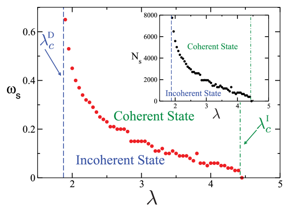
Additionally, the finite size of the system can also affect the thresholds of the hysteretic transition given the value of the inertia (Fig. 36). In comparison to the results obtained from the MFA in the limit of large network sizes $N$, $\lambda^{{\mathrm{I}}}_{c}$ increases steadily with $N$ and keeps constant for large inertia values. Interestingly, in the case of decreases in $\lambda$, $\lambda^{\mathrm{D}}_{c}$ remains nearly constant. For increasing $\lambda$, a good agreement of the critical coupling between simulations of large networks and the MFA is achieved at small $m$ but not at large $m$. The underlying mechanisms can be understood by the emergence of the secondary synchronization of drifting oscillators, which was firstly observed in [300]. Clusters of whirling oscillators (the secondary synchronization transition) are formed with an increase in the inertia were also observed in [307], and the emergence of the clusters can also be observed in random regular networks and in the high-voltage power grid in Italy. Note that in regular networks, where each degree is constant $k_{i}=k_{c}$ $\forall i$, the hysteretic loop enlarges with respect to increases in the fraction of connected links $k_{c}/N$.

Additionally to the research on hysteresis, the linear stability of the incoherent solution of the Kuramoto model with inertia with different natural frequency distributions was rigorously analyzed [308]. The critical coupling $\lambda_{c}$, where the system exhibits a first-order transition from non-synchronized to synchronized states, follows [309]

$$\frac{1}{\lambda_{c}}=\frac{\pi g(0)}{2}-\frac{m}{2}\int^{\infty}_{-\infty}\frac{g(\omega)}{1+m^{2}\omega^{2}}d\omega,$$ (308)

where $g(\omega)$ is unimodal with width $\Delta$. Without inertia, i.e. $m\rightarrow 0$, Eq. (308) reduces to the exact formula of the onset of collective synchronization of the first-order Kuramoto model (Eq. 9). For a Lorentzian $g(\omega)$, $\lambda_{c}$ is given by the following relation [307]

$$\lambda_{c}=2\Delta(1+m\Delta),$$ (309)

which is consistent with the results obtained in [308]. For a Gaussian distribution and with a rather small $m$, the first corrective terms are determined by [307]

$$\lambda_{c}=2\Delta\sqrt{\frac{2}{\pi}}\left\{1+\sqrt{\frac{2}{\pi}}m\Delta+\frac{2}{\pi}m^{2}\Delta^{2}+\sqrt{\left(\frac{2}{\pi}\right)^{3}-\frac{2}{\pi}}m^{3}\Delta^{3}\right\}+O(m^{4}\Delta^{4}).$$ (310)

With the increases in $m$ and $\Delta$ for the Lorentzian as well as the Gaussian distribution, it becomes harder and harder for the system to achieve complete synchronization [307].

Figure 36: Critical couplings $\lambda^{\mathrm{I}}_{c}$ and $\lambda^{\mathrm{D}}_{c}$ versus the network size $N$ with different values of $m$ in Eq. (302): (a) $m=0.8$, (b) $m=1$, (c) $m=2$ and $m=6$. In each panel, upper points indicate the value of $\lambda^{\mathrm{I}}_{c}$ and lower points indicate the value of $\lambda^{\mathrm{D}}_{c}$. In panels (a) and (b) with small $m$, the dashed black lines indicate the onset of collective synchronization obtained from Eq. 310. Adapted with permission from [307]. Copyrighted by the American Physical Society.

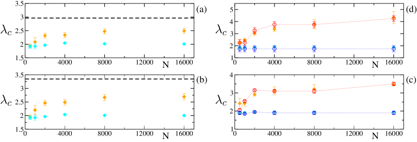
When the natural frequency distribution $g(\omega)$ is unimodal, symmetric, and has zero mean, the mean phase could be taken as a constant, e.g. $\psi(t)\equiv 0$. In the continuum limit, where $N\rightarrow\infty$, the fluctuations of $r(t)$ vanish and $r(t)$ therein is assumed to be constant, i.e. $r(t)\equiv r$. In this case, the system could be considered as a set of an one-node model. With respect to parameter values in the bifurcation diagram in Fig. 34, one oscillator could be located in the region of the stable limit cycle, of the stable fixed point or of bistability with the coexistence of two such stable solutions.

7.1.3 Mean-field theory with noise

Next, we briefly review the second-order Kuramoto model that includes noise:

$$\begin{split}\dot{\theta}_{i}&=\nu_{i}\\ m\dot{\nu}_{i}&=-\nu_{i}+\omega_{i}+\lambda r\sin{(\psi-\theta_{i})}+\xi_{i}(t),\end{split}$$ (311)

where $\xi_{i}(t)$’s are independent sources of Gaussian white noises, with $\left\langle\xi_{i}\right\rangle=0$ and correlation $\left\langle\xi_{i}(t)\xi_{j}(s)\right\rangle=2D\delta_{ij}\delta(t-s)$.

When $N\rightarrow\infty$, for the one-oscillator probability density, Acebrón and Spigler [296] considered the evolution equation of $\rho(\theta,\nu,\omega,t)$ as

$$\frac{\partial\rho}{\partial t}=\frac{D}{m^{2}}\frac{\partial^{2}\rho}{\partial\nu^{2}}-\frac{1}{m}\frac{\partial}{\partial\nu}\left[(-\nu+\omega+\lambda r\sin(\psi-\theta))\rho\right]-\nu\frac{\partial\rho}{\partial\theta},$$ (312)

where $\rho$ is normalized with $\int^{\infty}_{-\infty}\int^{\pi}_{-\pi}\rho(\theta,\nu,\omega,0)d\theta d\nu=1$. For identical oscillators, $g(\omega)=\delta(\omega)$, via setting the stationary solution $\rho(\theta,\nu)=\chi(\theta)\eta(\nu)$ and assuming that $\eta(\nu)$ is independent of $\lambda$ (motivated by numerical simulations [296]), the phase and frequency distributions are obtained explicitly from Eq. (312) and such results are validated by simulations [296]. In this case, the critical coupling from incoherence to coherence is independent of the inertia. For bimodal distributions of natural frequency, the inertia tends to destabilize incoherence and to harden the bifurcation from incoherence to synchronized states [308]. In particular, in the absence of inertia, the bifurcation is supercritical, but it becomes subcritical with increasing inertia.

Instead of Eq. (312), via averaging over the velocity $\nu(t)$ in the long-time limit, the Fokker-Planck equation for the probability distribution $\rho(\theta,\nu,\omega,t)$ can be reduced into the Smoluchowski equation, which yields [310, 311]

$$\frac{\partial\rho(\theta,t)}{\partial t}=\frac{\partial}{\partial\theta}\left[\left(\frac{\partial V(\theta)}{\partial\theta}\rho(\theta)+D\frac{\partial\rho(\theta)}{\partial\theta}\right)\left(1+m\frac{\partial^{2}{V(\theta)}}{\partial\theta^{2}}\right)\right],$$ (313)

with the washboard potential $V(\theta)\equiv-\lambda r\cos(\theta)-\omega\theta$. For $D=0$, by analyzing the stationary state of Eq. 313, the self-consistent equation is obtained [312]

$$r=\left(\frac{\pi}{2}-\frac{m}{2}\right)g(0)\lambda r+\frac{4}{3}mg(0)(\lambda r)^{2}+\frac{\pi}{16}g^{{}^{\prime\prime}}(0)(\lambda r)^{3}+O(\lambda r)^{4}.$$ (314)

In the presence of the inertia ($m\neq 0$), drifting oscillators as well as locked oscillators contribute to the phase coherence and the resulting quadratic term of the order $(\lambda r)^{2}$ induces hysteresis in the bifurcation diagram as observed before [300, 301]. The hysteresis is reduced with the presence of noise. The critical coupling strength increases monotonically with the increase of $D$ [312]. Moreover, via analyzing the power spectrum of the phase velocity, in contrast with synchronization suppressed by noise, the response of the phase velocity to the external driving is enhanced by a certain amount of noise [312]. Meanwhile, two related results were obtained: a consistent two-term Smoluchowski approximate equation in the limit of small inertia and the amplitude equation for an O(2)-symmetric Takens-Bogdanov bifurcation at the tricritical point of a standard Kuramoto model using the Chapman-Enskog method [311].

Recently, Gupta et al. [309] investigated coupled oscillator systems with inertia and noise in different situations. The dynamics studied in [309] written in the dimensionless form follows

$$\begin{split}\dot{\theta}_{i}&=\nu_{i}\\ \dot{\nu}_{i}&=-\frac{1}{\sqrt{m}}\nu_{i}+\delta\omega_{i}+r\sin{(\psi-\theta_{i}(t))}+\xi_{i}(t),\end{split}$$ (315)

where $\delta$ is the width of the frequency distribution $g(\omega)$. Given a realization of $g(\omega)$, where the set of oscillators consists of $N_{1}$ oscillators with frequencies $\omega_{1}$ and $N_{2}$ oscillators with frequencies $\omega_{2}$. When $\delta=0$, the stationary solution of $\rho(\theta,\nu)$ is

$$\rho_{\mathrm{st}}(\theta,\nu)\propto\mathrm{exp}\left[-\left(\nu^{2}/2-r\cos(\theta)\right)/D\right],$$ (316)

which corresponds to the canonical equilibrium and the stationary solution of the order parameter $r$ is determined by a self-consistent equation. For $\delta\neq 0$, the incoherent stationary state of $\rho_{\mathrm{inc}}(\theta,\nu,\omega)$ is

$$\rho_{\mathrm{inc}}(\theta,\nu,\omega)=\frac{1}{(2\pi)^{3/2}\sqrt{D}}\mathrm{exp}\left[(-\left(\nu-\delta\omega\sqrt{m}\right)^{2})/(2D)\right].$$ (317)

Interestingly, in terms of a linear stability analysis of the incoherent state, the stability threshold $\delta^{\mathrm{inc}}$ for the incoherent state in different situations can be obtained [309]. With $m\approx 0$ at fixed $D$, $\delta^{\mathrm{inc}}(m,D)$ satisfies

$$2=\int^{\infty}_{-\infty}\frac{Dg(\omega)d\omega}{D^{2}+\omega^{2}(\delta^{\mathrm{inc}}(0,D))^{2}}.$$ (318)

If $D\approx D_{c}=1/2$ then $\delta^{\rm{inc}}(m,D)\approx 0$. When $D\approx 0$ at fixed $m$, $\delta_{\mathrm{noiseless}}^{\mathrm{inc}}(m,D)$ satisfies

$$1=\frac{\pi g(0)}{2\delta^{\mathrm{inc}}_{\mathrm{noiseless}}}-\frac{m}{2}\int^{\infty}_{-\infty}\frac{g(\omega)d\omega}{1+m^{2}(\delta^{\mathrm{inc}}_{\mathrm{noiseless}})^{2}\omega^{2}}.$$ (319)

Komarov et al. [313] studied a generic model in the presence of inertia, noise, and phase shift, i.e.

$$m_{i}\ddot{\theta}_{i}=-\dot{\theta}_{i}+\omega_{i}+\lambda r\sin{(\psi-\theta_{i}-\varphi)}+\xi_{i}(t),$$ (320)

where the inertia $m_{i}$ is distributed according to the density function $f(m)$, and $\varphi$ is the phase shift. Rich phenomena emerge via considering various symmetry and asymmetry distributions of $f(m)$ and $g(\omega)$, e.g., the derivation of an exact solution of the self-consistent solution of the order parameter shows nontrivial phase transitions to synchrony due to correlations between natural frequencies and the moments of inertia [313].

Note that the recent review by Gupta et al. [314] provided a general mean-field analysis framework of the second-order Kuramoto model with noise, focusing on the equilibrium and out-of-equilibrium aspects of its dynamics from a statistical physics point of view.

7.1.4 Frequency-degree correlation

Let us now turn to effects of network topologies on dynamics. As illustrated in Sec. 5, the correlation between the dynamics and the structure can induce the emergence of dynamical abrupt phase transitions. In this case, the natural frequency distribution becomes asymmetric. Basnarkov and Urumov [233] investigated the first-order Kuramoto model with natural frequencies distributed according to a unimodal asymmetric function and showed that a first-order phase transition occurs if the distribution has a sufficiently large flat section. The MFA method [301, 300] (shown in the section 7.1.2) is provided for the second-order Kuramoto model (292) with symmetric frequency distribution, but the method for the model with asymmetric distribution is still open.

Ji et al. [244, 315] substantially extended the first-order Kuramoto model with frequency-degree correlation as discussed in Sec. 5 to the Kuramoto model with inertia. By considering $\omega_{i}$ of each oscillator $i$ proportional to its degree with zero mean, i.e. $\omega_{i}=B(k_{i}-\left\langle k\right\rangle)$ so that $\sum_{i}\omega_{i}=0$, the original dynamics becomes

$$\ddot{\theta}_{i}=-\alpha\dot{\theta}_{i}+B(k_{i}-\left\langle k\right\rangle)+\lambda\sum\limits^{N}_{j=1}A_{ij}\sin{(\theta_{j}-\theta_{i})},$$ (321)

where $B$ is a proportionality constant that weights the influence of the local structure on the natural frequencies. When $N\rightarrow\infty$, and in uncorrelated networks, after the transformation via replacing the coupling term by the imaginary term of the continuum-limit version of $r$ (Eq. 175), Eq. (321) becomes

$$\ddot{\theta}=-\alpha\dot{\theta}+B(k-\left\langle k\right\rangle)+k\lambda r\sin(\psi-\theta),$$ (322)

where the subscript _i is dropped in the continuum limit.

In the mean-field version (322), each oscillator appears to be uncoupled from the others but interacts through the mean-field properties $(r,\psi)$ and the phase $\theta$ is pulled toward $\psi$ by the coupling strength $k\lambda r$. Natural frequencies are proportional to degrees, and since the degree distribution is not necessary symmetric, $\psi$ cannot be set as a constant, but rather oscillates periodically. Here, we assume that $r$ is at the steady state, otherwise, complex phenomena could occur, e.g. secondary synchronization [300, 307]. To derive sufficient conditions for synchronization, for convenience, a new rotating reference is defined as $\phi=\theta-\psi$. Substituting this into Eq. (322) yields

$$\ddot{\phi}=-\alpha\dot{\phi}+B[k-\left\langle k\right\rangle-C(\lambda r)]-k\lambda r\sin\phi,$$ (323)

where $C(\lambda r)\equiv(\ddot{\psi}+\alpha\dot{\psi})/B$. In this case, each oscillator can be treated separately and behaves independently, i.e. either synchronizes to the mean-field or runs periodically with frequency given by Eq. (300), which further depends on the parameter combination that includes the dissipation coefficient $\alpha$, the new natural frequency $B[k-\left\langle k\right\rangle-C(\lambda r)]$ and the new coupling strength $k\lambda r$.

Provided that nodes with degree within the range $[k_{1},k_{2}]$ are synchronized, i.e. $\dot{\phi}=0$ and $\ddot{\phi}=0$, their phases are $k$-dependent with $\phi=\arcsin\left(\frac{B\left(k-\left\langle k\right\rangle-C(\lambda r)\right)}{k\lambda r}\right)$ and the density function $\rho(\phi|k)$ can be rewritten as $\rho(\phi|k)=\delta\left[\phi-\arcsin\left(\frac{B\left(k-\left\langle k\right\rangle-C(\lambda r)\right)}{k\lambda r}\right)\right]\mbox{ for }k\in\left[k_{1},k_{2}\right]$. After substituting the density function into the definition of the order parameter (see Sec. 2), the locked order parameter $r_{\mathrm{lock}}$ follows

$$r_{\mathrm{lock}}=\frac{1}{\left\langle k\right\rangle}\int_{k_{1}}^{k_{2}}\int_{0}^{2\pi}P(k)ke^{i\phi(t)}\delta{\left[\phi-\arcsin{\left(\frac{B(k-\langle k\rangle-C(\lambda r))}{k\lambda r}\right)}\right]}d\phi dk,$$

(324)

and its real term becomes

$$r_{\mathrm{lock}}=\frac{1}{\left\langle k\right\rangle}\int_{k_{1}}^{k_{2}}\left.kP(k)\sqrt{1-\left(\frac{B\left(k-\left\langle k\right\rangle-C(\lambda r)\right)}{k\lambda r}\right)^{2}}\right.dk.$$ (325)

Figure 37: Parameter space of one-node model for the increasing coupling strength (a) and for the decreasing coupling strength (b). The red (dark) region indicates the existence of the stable fixed point (the stable limit cycle). Adapted with permission from [315]. Copyrighted by the American Physical Society.

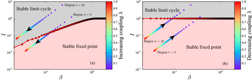
On the other hand, nodes with $k\in k_{\mathrm{drift}}\equiv\left[k_{\min},k_{1}\right]\cup\left[k_{2},k_{\max}\right]$ are drifting, where $k_{\min}$ denotes the minimal degree and $k_{\max}$ the maximal degree. These drifting nodes rotate with the period $\hat{T}$ and the frequency $\hat{\omega}=\frac{2\pi}{\hat{T}}$ in the stationary state. As the density $\rho_{\rm{drift}}(\phi,t|k)$ is proportional to $|\dot{\phi}|^{-1}$ [300, 301] and $\oint\rho_{\rm{drift}}(\phi|k)d\phi=\int^{\hat{T}}_{0}\rho_{\rm{drift}}(\phi|k)\dot{\phi}dt=1$, we get $\rho_{\rm{drift}}(\phi|k)=\hat{T}^{-1}|\dot{\phi}|^{-1}=\frac{\hat{\omega}}{2\pi}|\dot{\phi}|^{-1}$. Therefore, the drifting order parameter $r_{\mathrm{drift}}$ becomes

$$r_{\mathrm{drift}}=\frac{1}{2\pi\left\langle k\right\rangle}\int_{k\in k_{\mathrm{drift}}}\int^{\hat{T}}_{0}kP(k)\hat{\omega}|\dot{\phi}|^{-1}e^{i\phi(t)}\dot{\phi}dtdk.$$ (326)

As nodes with negative (positive) natural frequency oscillate over (under) the locked group, one can assume that $\dot{\phi}<0$ for $k\in\left[k_{\min},k_{1}\right]$ and $\dot{\phi}>0$ for $k\in\left[k_{2},k_{\max}\right]$ without loss of generality. A perturbation approximation of the self-consistent equations enables us to get a series expression of the periodic solution $\phi(t)$ using the Poincare-Lindstead method and approximate $\cos(\phi(t))$ using Bessel functions [301]. After performing some manipulations on Eq. (326) motivated by [300], one gets the final solution of the real part of $r_{\text{drift}}$ as follows

$$r_{\mathrm{drift}}=\left(-\int_{k_{\min}}^{k_{1}}+\int_{k_{2}}^{k_{\max}}\right)\frac{-rk^{2}\lambda\alpha^{4}P(k)}{B^{3}\left[k-\left\langle k\right\rangle-C(\lambda r)\right]^{3}\left\langle k\right\rangle}dk.$$ (327)

The self-consistent equation of $r$ sums the contribution $r_{\mathrm{lock}}$ (325) from oscillators locked to the mean-field and the contribution $r_{\mathrm{drift}}$ (327) from the rest, i.e. $r=r_{\mathrm{lock}}+r_{\mathrm{drift}}$. To solve this self-consistent equation, three parameters remain to be solved: constant $C$ and the range of the degree of synchronized nodes $[k_{1},k_{2}]$. Considering the complex order parameter summing Eqs. (324) and (326) and following a similar procedure to express $\int_{0}^{\hat{T}}\cos\phi(t)dt$ [301] for the integral $\int_{0}^{\hat{T}}\sin\phi(t)dt$ in its imaginary term, we yield the self-consistent equation

$$0 = \frac{1}{\left\langle k\right\rangle}\int_{k_{1}}^{k_{2}}kP(k)\frac{B(k-\langle k\rangle-C(\lambda r))}{k\lambda r}dk$$ (328)

$$+\frac{1}{2\left\langle k\right\rangle}\left(\int_{k_{\min}}^{k_{1}}+\int_{k_{2}}^{k_{\max}}\right)\frac{rk^{2}\lambda\alpha^{2}P(k)}{B^{2}\left[k-\left\langle k\right\rangle-C(\lambda r)\right]^{2}}dk$$

Given the variable $\lambda r$, $C(\lambda r)$ can be taken as a function of $k_{1}$ and $k_{2}$.

In order to determine these quantities, for notational simplicity, we set $\beta\equiv\alpha/\sqrt{k\lambda r}$ and $I\equiv B(k-\left\langle k\right\rangle-C(\lambda r))/(k\lambda r)$. As depicted in panel (a) of Fig. 37, initially all nodes are in the region of the stable limit cycle with increasing $\lambda$ until the onset of synchronization $\lambda^{\mathrm{I}}_{c}$. At $\lambda^{\mathrm{I}}_{c}$, the homoclinic bifurcation occurs and nodes within the synchronization boundary start synchronizing to the mean-field. For small value of $\beta$, $[k^{\mathrm{I}}_{1},k^{\mathrm{I}}_{2}]$ must fulfil two conditions: $\frac{\left|B\left(k-\left\langle k\right\rangle-C(\lambda r)\right)\right|}{k\lambda r}\leq 1$ and $\frac{\left|B\left(k-\left\langle k\right\rangle-C(\lambda r)\right)\right|}{k\lambda r}\leq\frac{4\alpha}{\pi\sqrt{k\lambda r}}.$

Figure 38: Analytical (in blue) and numerical (in red) results of the order parameter $r$ with increasing and decreasing strength (a) and $C(\lambda r)$ with increasing coupling strength (b) for synchronization diagrams. Adapted with permission from [244]. Copyrighted by the American Physical Society.

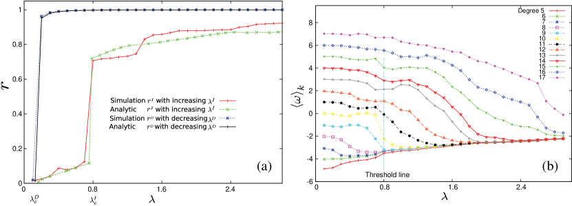
For decreasing $\lambda$, nodes start from the phase-locked synchronous state (panel (b) in Fig. 37). With decreasing in $\lambda$, nodes reach the asychronous state at $\lambda^{\mathrm{D}}_{c}$, at which a saddle-node bifurcation occurs. Therefore, the phase-locked oscillators satisfy $\frac{\left|B\left(k-\left\langle k\right\rangle-C(\lambda r)\right)\right|}{k\lambda r}\leq 1$ and the synchronization boundary follows $[k_{1}^{\mathrm{D}},k_{2}^{\mathrm{D}}]\equiv\left[\frac{\left\langle k\right\rangle+C(\lambda r)}{1+\frac{\lambda r}{B}},\frac{\left\langle k\right\rangle+C(\lambda r)}{1-\frac{\lambda r}{B}}\right].$ With the above synchronization boundary $[k_{1},k_{2}]$, the self-consistent equation of the order parameter can be obtained as a sum of Eqs. 325 and 327 as a function of $C$, $k_{1}$ and $k_{2}$. Additionally, the imaginary term of the complex order parameter (328) should then be used to obtain the dependence $C=C(\lambda r)$. The comparison between analytical results of the order parameter and simulations are shown in Fig. 38 (a).

To further uncover the first-order phase transition [Fig. 38 (a)], the average frequency $\left\langle\omega\right\rangle_{k}$ of nodes with the same degree $k$ (here called cluster) is visualized as a function of the coupling strength $\lambda$, and its calculation follows

$$\left\langle\omega\right\rangle_{k}=\sum_{[i|k_{i}=k]}\langle\dot{\theta}_{i}\rangle_{t}/(NP(k)),$$ (329)

where $\langle\dot{\theta}_{i}\rangle_{t}=\int^{t+T}_{t}\dot{\theta}_{i}(\tau)dt/T$. Unlike explosive synchronization in [30] and as discussed in Sec. 5 (see Fig. 19), where all nodes synchronize abruptly at the same coupling, a new phenomenon was found. Oscillators join the synchronous component grouped into clusters of nodes with the same degree, where small degree nodes form the synchronous component simultaneously, whereas high degree nodes synchronize successively (see Fig. 38). This phenomenon was termed cluster explosive synchronization [244, 315].

7.1.5 Further works

Additionally, research has been done related to models with time delay [316], with periodic driving [317] and chimera states [318, 319].

(i) Time delay: Finite inertia and time delay are related in some systems, e.g., finite-time interval required for transforming information in a superconducting junction network [320] and in coupled nonlinear electronic circuits [321]. The interplay between inertia and time delay was analytically and numerically investigate [322], where the emergence of spontaneous phase oscillation without external driving was reported. Such spontaneous oscillation was found to suppress synchronization and its frequency was observed to decrease when inertia and time delay decreased. Moreover, the phase diagram can be analytically obtained (in the three-dimensional space of inertia, time delay and coupling strength), where oscillatory and stationary states appear.

Another recent contribution studied the onset of synchronization in a star network of the second-order Kuramoto model with frequency-degree correlation in the presence of a time delay. The model is governed by [316]

$$m\ddot{\theta}_{i}=-\dot{\theta}_{i}+\omega_{i}+\frac{\lambda}{N}\sum\limits^{N}_{j=1}\sin{(\theta_{j}(t-\tau)-\theta_{i}(t))},$$ (330)

where $\omega_{i}=k_{i}$ and $\tau$ denotes the time delay. To address the effects of $\tau$ on the collective synchronization, a mean-field analysis was conducted following the same analytical process of [243], yielding a good approximation between numerical results and the MFA. However, the results need to be further investigated to include the influences of the inertia $m$ on the onset of synchronization.

(ii) External periodic forcing: To understand effects of inertia on the collective synchronization in a set of coupled oscillators with external driving, consider the following dynamics [317]

$$m\ddot{\theta}_{i}=-\dot{\theta}_{i}+\omega_{i}+\lambda r\sin{(\psi-\theta_{i}(t))}+I_{i}\cos{(\Omega t)},$$ (331)

where $I_{i}\cos{(\Omega t)}$ describes the periodic driving on the $i$-th oscillator. In the absence of inertia ($m=0$), only oscillators locked to the external driving contribute to the collective synchronization. Otherwise, with inertia ($m\neq 0$), drifting oscillators as well as oscillators locked to the external driving contribute to the collective synchronization. It was shown analytically that the inertia tends to suppress synchronization [317].

(iii) Chimera states: Jaros et al. [318] illustrated different types of chimera states in the Kuramoto model with inertia and its dynamics follows

$$m\ddot{\theta}_{i}=-\dot{\theta}_{i}+\frac{\lambda}{2L+1}\sum^{i+L}_{j=i-L}\sin{(\theta_{j}(t)-\theta_{i}(t)-\varphi)},$$ (332)

where $\varphi$ indicates the phase lag and each node is linked to its $L$ nearest neighbors to the left and to the right. A different type of spatiotemporal pattern was defined, termed imperfect chimera states, where a small number of oscillators escapes from the synchronized cluster. Moreover, by varying $\varphi$, the transition of chimera states from coherence to incoherence was observed.

Additionally, note that effects of assortative mixing on synchronization are worth to being investigated. We saw in Sec. 3.2 that the combination of mean-field theory and the OA ansatz on the first-order Kuramoto model with frequency-degree correlation can yield a good approximation to discover the influence of topology on collective synchronization [96]. It would be interesting to combine recent developments on the low-dimensional behavior of the second-order Kuramoto model [289] with the approach in [96] in order to further analyse the recent results obtained on assortative networks of second-order Kuramoto oscillators [323]. Moreover, effects of shortcuts in SW networks on synchronization remain to be further explored [324].

7.2 Basin stability

In the last decades, much research effort has been devoted to explore how the synchronizability of a network of coupled oscillators depends on network topology [325, 14], but from a local perspective, related to spectral properties of the underlying structure. The seminal work [326] initiated a new line of research by proposing a new stability approach that is related to the size of the basin of attraction for a synchronous state. Two additional questions were posed: How likely will a network fall into sync, starting from random initial conditions? And how does the likelihood of synchronization depend on the network topology? Alternatively, the first question can be addressed differently [327, 34]: How likely will a network return to the synchronous state after even large random perturbations? Substantially, the correlation was investigated between basin stability and the network architecture in the second-order Kuramoto model [302]. In this subsection, we review the basin stability formalism and the main results obtained so far.

7.2.1 Basin stability formalism

Traditional linear stability is too local to adequately quantify in many applications how stable a state is [34]. A new concept was defined, termed basin stability ($\mathcal{BS}$), which quantifies the likelihood that a system will retain a desirable state after even large perturbations [327, 34]. Basin stability is non-local, nonlinear and easily applicable to high-dimensional systems, even with fractal basin boundaries. It is related to the volume of the basin of attraction. The concept of $\mathcal{BS}$ can be easily applied to high-dimensional systems as complex networks [327, 34, 302].

To quantify how stable a synchronous state of the networked Kuramoto model with inertia (292) is against large perturbations depending on network topologies, the basin stability $\mathcal{BS}_{i}$ at each node $i$ is defined as [34, 302]

$$\mathcal{BS}_{i}=\int\chi(\theta_{i},\nu_{i})\rho_{\rm{p}}(\theta_{i},\nu_{i})d\theta_{i}d\nu_{i},$$ (333)

with $\theta_{j}(0)=\theta^{*}_{j}$ and $\nu_{j}(0)=0$ for all $j\neq i$ where $\chi(\theta_{i},\nu_{i})$ is an indicator function with $\chi(\theta_{i},\nu_{i})=1$ if $(\theta_{i},\nu_{i})$ belongs to its basin of attraction of the synchronous state, and $\chi(\theta_{i},\nu_{i})=0$, otherwise. $\rho_{\rm{p}}$ is a perturbation density function with the normalization condition $\int\rho_{\rm{p}}(\theta_{i},\nu_{i})d\theta_{i}d\nu_{i}=1$. $\theta_{j}(0)=\theta^{*}_{j}$ and $\nu_{j}(0)=0$ for all $j\neq i$ indicate that initially all nodes are in the synchronous state except $i$. The value of $\mathcal{BS}_{i}$ at node $i$ expresses the likelihood that the system returns to the synchronous state after $i$ having been subjected to (large) perturbations. Specifically, $\mathcal{BS}_{i}=0$ when the node $i$ is unstable, and $\mathcal{BS}_{i}=1$ when $i$ is globally stable.

Numerically, $\mathcal{BS}_{i}$ is estimated by means of a Monte-Carlo method. More specifically, the dynamics is integrated independently for $M_{i}$ different initial conditions drawn according to $\rho_{\rm{p}}$, one can count the number $S_{i}$ of initial conditions at which the system converges to the synchronous state and calculate $\mathcal{BS}$ as [302]

$$\mathcal{BS}_{i}=\frac{S_{i}}{M_{i}}.$$ (334)

This is a repeated Bernoulli experiment, and thus the standard error $e$ of $\mathcal{BS}$ follows

$$e=\frac{\sqrt{\mathcal{BS}_{i}(1-\mathcal{BS}_{i})}}{M_{i}},$$ (335)

which turns out to be independent of the system’s dimension, making $\mathcal{B}S$ easily applicable to high-dimensional systems [302].

7.2.2 Basin stability approximation

As an illustration, we consider the one-node model (293) [327, 302], The basic dynamics of the one-node model is shown in Sec. 7.1.1. Here we focus on evaluating the volume of the attracting basin of the synchronous state. In Fig. 39, the basin of attraction of the synchronous state with respect to $\alpha$ is plotted in panels (a-c) and its volume increases with $\alpha$ until the critical value $\alpha_{c}=\frac{\pi\omega}{4\sqrt{\lambda}}$ obtained from (297), at which the homoclinic bifurcation occurs (shown in the bifurcation diagram Fig. 34). Correspondingly, basin stability $\mathcal{BS}$ increases with $\alpha\in(0,\alpha_{c})$ from Fig. 39 (a) to (b) and then persists at $\mathcal{BS}=1$ with $\alpha>\alpha_{c}$ as shown in Fig. 39(d). Considering a simple case where $\rho_{\rm{p}}(\theta,\nu)$ is uniformly distributed within the region of $(\theta,\nu)\in[-\pi,\pi]\times[-\epsilon,\epsilon]$ with $\epsilon=100$ and $\mathcal{BS}$ therein is proportional to the volume of the basin of attraction of the fixed point.

Figure 39: State space of the model (293) with $\alpha=0.1$ (a), $\alpha=0.27$ (b) and $\alpha=0.3$ (c) at $\omega=1$ and $\lambda=8$. The basin of attraction of the stable fixed point $\theta^{*}$ is colored green, and that of the stable limit cycle is colored red. (d) Basin stability $\mathcal{BS}$ obtained from Eq. (334) of the synchronous state versus the the damping parameter $\alpha$. Here $\rho(\theta,\nu)$ is a uniform distribution restricted to a lox $(\theta,\nu)\in[-\pi,\pi]\times[-100,100]$. Adapted from [327].

Note that in Fig. 39(d), basin stability $\mathcal{BS}$ increases almost linearly with $\alpha$ in the interval $(0,\alpha_{c}]$. Provided that the linear correlation between $\mathcal{BS}$ and $\alpha$ validates within the region of bistability given other values $\omega$ and $\lambda$, Ji et al. [328] estimated $\mathcal{BS}(\alpha,\omega,\lambda)$ with respect to $\alpha$, $\omega$ and $\lambda$.

Firstly, when the system is weakly dissipated with $\alpha\approx 0$ denoted by $\alpha_{0}$, the volume of the fixed point’s basin ensembles all the librations and the basins’ boundary is tangent to the stable manifold of the saddle $(\theta^{*}_{2},\nu^{*}_{2})$. Observed numerically that the basin is symmetrical. According to the energy function (294), the upper $\nu_{+}$ and the lower $\nu_{-}$ boundaries are approximated by $\nu_{\pm}\approx\pm\sqrt{2(\omega\theta+\lambda\cos(\theta)+E(\theta^{*}_{2},\nu^{*}_{2}))}$. Therefore, the approximation of $\mathcal{BS}(\alpha_{0},\omega,\lambda)$ at weakly dissipated system follows [328]

$$\mathcal{BS}(\alpha_{0},\omega,\lambda)\approx\int^{\theta^{*}_{2}}_{\theta_{0}}(\nu_{+}-\nu_{-})/(4\epsilon\pi)d\theta,$$ (336)

where $4\epsilon\pi$ is taken for normalization and $\theta_{0}$ is the left joint point between the lower and upper basin boundary, satisfying $0=\sqrt{2(\omega\theta_{0}+\lambda\cos(\theta_{0})+E(\theta^{*}_{2},\nu^{*}_{2}))}$ with $\theta_{0}\neq\theta^{*}_{2}$.

At $\alpha_{c}$, the upper basin boundary is tangent to the curve of the limit cycle. Thanks to the approximation of the limit cycle curve (300), the upper basin boundary follows $\omega/\alpha_{c}+f(\theta,\alpha_{c},\omega,\lambda)$, where $f(\theta,\alpha_{c},\omega,\lambda)=\frac{\lambda\alpha^{2}}{\alpha^{4}+\omega^{2}}(\frac{\omega}{\alpha}\cos(\theta)-\alpha\sin(\theta))$. As numerically observed that the state space under the upper line belongs to the attracting basin of the stable fixed point. Therefore, at the onset $\alpha_{c}$, $\mathcal{BS}(\alpha_{c},\omega,\lambda)$ is approximated as [328]

$$\mathcal{BS}(\alpha_{c},\omega,\lambda)\approx\int^{\pi}_{-\pi}\frac{\omega/\alpha_{c}+f(\theta,\alpha_{c},\omega,\lambda)+\epsilon}{4e\epsilon\pi}.$$ (337)

Therefore, given the linear correlation between $\mathcal{BS}$ and $\alpha\in[\alpha_{0},\alpha_{c}]$, $\mathcal{BS}$ is defined as a function of $\alpha$, $\omega$ and $\lambda$ [328]

$$\mathcal{BS}(\alpha,\omega,\lambda)\approx\frac{\mathcal{BS}(\alpha_{0},\omega,\lambda)-\mathcal{BS}(\alpha_{c},\omega,\lambda)}{\alpha_{0}-\alpha_{c}}(\alpha-\alpha_{0})+\mathcal{BS}(\alpha_{0},\omega,\lambda),$$ (338)

for $\alpha\in[\alpha_{0},\alpha_{c}]$ and $\mathcal{BS}(\alpha,\omega,\lambda)=1$ for $\alpha>\alpha_{c}$.

By definition Eq. (333), $\mathcal{BS}$ depends on the choice of the probability density of random perturbations $\rho_{\rm{p}}(\theta,\nu)$. The formula of $\mathcal{BS}$ Eq. (338) is derived given the linear correlation between $\mathcal{BS}$ and the dissipation parameter $\alpha$ when the perturbations are uniformly distributed within a region, which was firstly considered for convenience. The Gaussian distribution $\rho_{\rm{p}}(\theta,\nu)=\frac{1}{(2\pi)^{3/2}b}\mathrm{exp}\left(-\frac{\nu^{2}}{2b^{2}}\right)$ was also considered in [329]. Given parameter values in the region of bistability, the dependence of $\mathcal{BS}$ on the width $b$ of $\rho$ was investigated. At small $b$, $\mathcal{BS}$ persists at a high value. With the increases in $b$ beyond a critical value, $\mathcal{BS}$ decreases sharply and then remains at almost small constant values with high values of $b$.

Basin boundaries can be either smooth, e.g. intricately intertwined shapes in panel (a) and (b) of Fig. 39 or fractal [329]. Fractal basin boundaries can strongly influence the predictability of which attractor a system eventually converge. Suppose that the measurement of initial conditions has an uncertainty $\varepsilon$, if the initial conditions close to fractal basin boundaries, it is uncertain to which attractor the system will converge. This causes some trouble when estimating $\mathcal{BS}$ in the long-term behaviour. The simple damped pendulum with periodic driving was considered and it was shown that $\mathcal{BS}$ estimation is robust, i.e. $\mathcal{BS}$ can be applicable to nonlinear dynamical systems even with fractal basin boundaries [329].

7.2.3 Correlation with network topology

Figure 40: Relation between single-node basin stability $\mathcal{BS}$ and network topologies. (a) The histogram of $\mathcal{BS}_{i}$ for all nodes in the assemble. Most nodes have fair basin stability delimited by two dotted lines. Average basin stability $\left\langle\mathcal{BS}\right\rangle$ with respect to degree (b), average degree of neighbors of nodes with degree $k=1$ and $k=2$ (c) and that of nodes with degree $k=3$ and $k=4$ (d). $\left\langle\mathcal{BS}\right\rangle$ with respect to shortest-path betweenness $b$ (d). Some illustrations of nodes with certain distinct values of $b$. Adapted from [302].

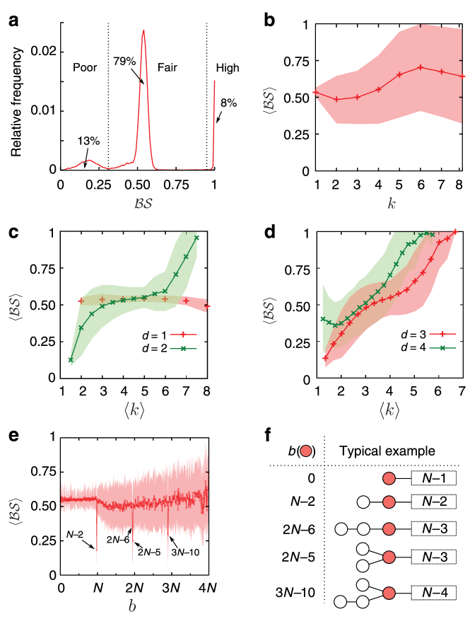
To reveal the relation between stability and network structure, in [302, 327] an ensemble of $1,000$ randomly generated networks with average degree $\left\langle k\right\rangle=2.7$ was statistically studied. Furthermore, two types of natural frequency are selected with $N/2$ nodes with positive natural frequency $\omega_{i}=+1$ and $N/2$ nodes with negative natural frequency $\omega_{i}=-1$. The histogram of the single-node basin stability $\mathcal{BS}$ is given in Fig. 40 showing that most nodes have a fair value of $\mathcal{BS}$. More interesting and special are nodes with poor basin stability ($\mathcal{BS}<0.3$) resp. high basin stability ($\mathcal{BS}>0.95$). To uncover these special nodes, the authors averaged basin stability $\left\langle\mathcal{BS}\right\rangle$ of all nodes having the same degree $k$ in Fig 40(b). Unlike initial expectations, nodes with higher $k$ do not have larger $\left\langle\mathcal{BS}\right\rangle$. A more insightful characteristic is shown in Fig. 40(c-d). Average $\mathcal{BS}$ increases with the average degree $\left\langle k\right\rangle_{k}$ of neighbors of nodes with degree $k\geq 2$ except nodes with $k=1$. The main conclusions are obtained from the characteristic shown in Fig. 40(e): $\left\langle\mathcal{BS}\right\rangle$ as a function of the shortest path and betweenness $b$. Most $b$’s have no certain effects on $\left\langle\mathcal{BS}\right\rangle$. Interestingly, certain $b$’s, indicated by arrows, have extremely low values of $\mathcal{BS}$. Fig. 40(f) sketches some examples of typical nodes in red with such betweenness $b$. These nodes are the so-called dead ends or dead trees and strongly diminish the stability of the network [302].

The stability of a system with varying network topologies was also investigated given a bipolar natural distribution [302]. Actually, for fixed networks, the stability also varies with the topological localization of $\omega_{i}$. For example, both the values of $\omega_{i}$ of a given node $i$ and its topological localization affects phase coherence in the networked Kuramoto model with a bipolar distribution of $\omega_{i}$. Furthermore, synchronization can be enhanced when nodes are surrounded by nodes with opposite $\omega_{i}$ [330]. Therefore, it is interesting to investigate how the localization of generators and consumers influences the stability of power grids.

Schultz et al. [331] further investigated the relationship between stability and topological properties using a random growth model and other spatially embedded infrastructure networks [332]. Such a model reproduces various network characteristics and provides a wide range of network topologies. The dynamics is based on the classical Kuramoto model with inertia but with weighted coupling strength as follows [331]

$$\ddot{\theta}_{i}=-\alpha\dot{\theta}_{i}+\omega_{i}+\sum\limits^{N}_{j=1}\lambda_{ij}\sin{(\theta_{j}-\theta_{i})},$$ (339)

where $\lambda_{ij}$ is determined by the voltage amplitudes and generator constants, and it is also related to the link weights, precisely $\lambda_{ij}\propto\frac{1}{X_{ij}}$, where $X_{ij}$ are determined by the entries of the reactance matrix. A statistical analysis using a Monte-Carlo rejection method was used to investigate the influence of network motifs, including four-size motifs, dead tree gateways and detours, on the stability of networks. Dead tree gateways are termed to refer an ensemble of nodes within dead trees, e.g. red nodes in Fig. 40(f). Detour nodes are nodes in triangles with very low shortest-path betweenness [331]. Characteristics of nodes on detours are with degree two and with unit value of the clustering coefficient. If networks are resistance, these nodes take a significant amount of transformations. In comparison to [327, 302], where only poor $\mathcal{BS}$’s are detected in terms of shortest-path betweenness, downward and upward peaks of the curve of single-node basin stability were observed with respect to the vertex current flow betweenness (VCFB) as shown in Fig. 41. The appearance of detour nodes seems to prevent poor local basin stability and the identification of them is very important for enhancing the whole network stability. Moreover, due to costly simulations, e.g. $100,000\times 500$ times simulations used in [302], the strategy to estimate that $80\%$ of nodes are neither dead tree gateways nor detour nodes shows a good agreement with numerical results [331].

From the above various analysis, we can learn that it could be possible to uncover specific correlation between stability and local structures given a specific system with fixed configurations, but the results can be varied depending on the stability methods. It should be noted, however, that $\mathcal{BS}$ is a first-order method. In order to deepen the understanding of stability in different contexts, e.g., in partial synchronization, more subtle definitions should be considered. Progress in this direction has been made recently [333, 334].

Figure 41: Single-node basin stability versus the vertex current flow betweenness (VCFB). The four red dotted lines indicates poor basin stability of dead tree gateways. The line’s color indicates the share of nodes in detours with the respective betweenness value. The shade indicates the standard derivation. The inset sketches a detour motifs with the detour node colored in blue. From [331]

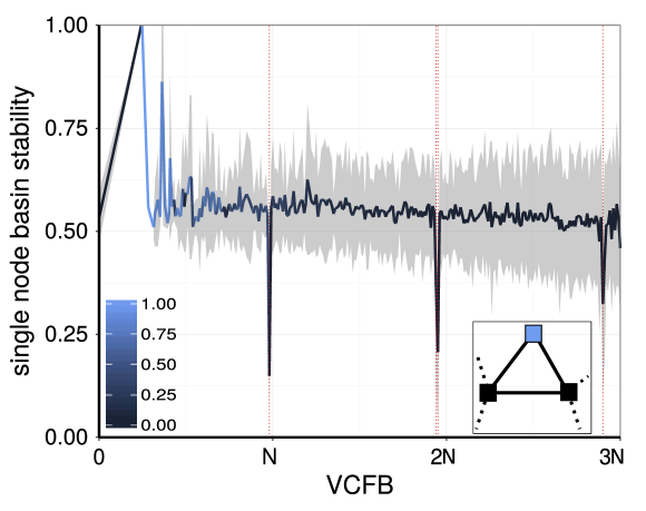
8 Optimization of synchronization

The observation that the level of synchronization depends on networks structure has motivated questions about the optimal topology to reach the highest synchronization level. Gleiser and Zanette [335] considered the Kuramoto model, in which the dynamics of each oscillator is described by the equations (11) with $\lambda_{ij}=\lambda/k$ (see Sec. 2). On a time interval of length $T$, the average oscillation frequency is defined by $\omega_{i}^{\rm{eff}}=\frac{1}{T}\int_{t}^{t+T}\dot{\theta_{i}}(t^{\prime})dt^{\prime}$. If the coupling between two oscillators is sufficiently strong, the synchronous state $\omega_{i}^{\rm{eff}}=\omega_{j}^{\rm{eff}}$ is reached for $T\to\infty$.

The network adaptation is performed by the following procedure [335]. After the time interval $T$ is past, a node $i$ is selected at random. The difference $\delta_{ij}=|\omega_{i}^{\rm{eff}}-\omega_{j}^{\rm{eff}}|$ is calculated for all $j\neq i$. The oscillator $k$ for which $\delta_{ik}$ is minimum is selected. If $k$ is a neighbour of $i$, the network is not changed. Otherwise, it is selected, amongst the neighbors of $i$, the node $l$ for which $\delta_{il}$ is maximum. Then, the connection between $i$ and $l$ is replaced by a link between $i$ and $k$. After this update, the process is repeated until a stationary state is attained. For practical purposes, the authors assumed that the procedure is executed only if the maximal difference between the average frequencies of oscillator $i$ and all its neighbours $m$ is higher than a defined threshold.

By considering a random homogeneous network, the authors verified that the connections are changed in order to create and keep connections between oscillators that are more likely to become synchronized [335]. In addition, they verified that the clustering coefficient is changed during the adaptive process. For small values of order parameter, the clustering coefficient is almost unchanged. The same behavior is verified for strong coupling strengths. However, for intermediate values, the clustering presents a maximum, which indicates that the resulting network acquires a more structured (less random) organization. The analysis of the mean distance, reinforce that the network structure moves from a random topology to a SW network [335]. In fact, the authors verified that the network evolution creates cluster of densely connected nodes, which are formed by mutually synchronized oscillators. The occurrence of these clusters decreases the mean distance of the network.

To complement the analysis by Gleiser and Zanette [335], Brede [336] studied the relation between the native frequency of the oscillators and the organization of optimized networks of Kuramoto oscillators. He defined that a network $A_{1}$ is more synchronizable than a network $A_{2}$ if the order parameter $r_{A_{1}}(\lambda)>r_{A_{2}}(\lambda)$ for all $\lambda$. To optimize the network structure, he proposed the following procedure. For a fixed value of the coupling strength $\lambda^{*}$, a network is adapted by a rewiring in the coupling’s network configuration. More specifically, a random chosen link is rewired and this rewiring is accepted if the average fitness $\overline{r}(t,\lambda^{*})=(1/\Delta t)\sum_{t=T_{\rm{rel}}}^{T_{\rm{rel}}+\Delta t}r(t,\lambda^{*})$ is increased. $T_{\rm{rel}}$ is the number of time steps for relaxation. This process is repeated until no move was accepted during $2\sum_{ij}A_{ij}$ interactions. It was verified that to obtain optimal networks, native frequencies of adjacent oscillators must be anti-correlated [336]. Furthermore, if the network structure remains fixed and optimization is performed by swapping the natural frequencies of adjacent oscillators instead of by link rewiring, a positive correlation between frequencies and degrees emerges, yielding even higher levels of synchronization (see Sec. 5). Therefore, the level of synchronization depends not only on the network structure, but also on the assignment of frequencies to nodes [336] (a similar study as in [336] has been recently carried out by considering a simulated annealing method [337]). Moreover, he verified that the optimized networks are very small, homogeneous and no cliquish. This result is in contrast with those in [335], in which the authors verified that networks are characterized by a high level of cliquishness and large average distances. This analysis was further extended in [137], where it was demonstrated that the previous observations are also valid in the thermodynamic limit. He confirmed that the synchronization properties depend on both the coupling topology and network structure.

In a subsequent paper, Brede [338] considered the same method as in [336] to analyze local synchronization and the onset of synchronization by adapting the network structure. However, a measure of synchronization given by a combination of the global order parameter and the measure of pairwise coherence of links as a local measure of synchronization was assumed [273],

$$r_{\mathrm{link}}=\frac{1}{E}\sum_{k,l}\Big{|}\lim_{\Delta T\to\infty}\frac{1}{\Delta T}\int_{\tau_{r}}^{\tau_{r}+\Delta T}e^{i(\phi_{l}(t)-\phi_{k}(t))dt}\Big{|},$$ (340)

where $E$ is the total number of links, $\tau_{r}$ represents the relaxation time (see Sec. 2.3) and $\Delta T$ is the time over which the coherence between adjacent oscillators is measured. This measure was used to detect community structures in networks [14, 153, 156, 157]. Notice that a network can present $r_{\mathrm{link}}\simeq 1$ even when $r\ll 1$. The synchronization of the network is measured by

$$\mathcal{F}(\lambda^{*})=br(\lambda^{*})+(1-b)r_{\mathrm{link}}(\lambda^{*}),$$ (341)

where $b$ is a constant that balances the contribution of the global and local synchronization. The author considered $b=1/2$ in most of the analysis presented in [338].

By considering ER networks as the starting topology for the adaptation process, the connections were rewired in order to increase $\mathcal{F}$. Brede [338] verified that depending on the coupling $\lambda^{*}$, considered as a fixed parameter during the network adaptation, the optimized network presents different properties. As we can see in Fig. 42, for small coupling, the optimized network presents modular organization. These modules are formed by nodes presenting similar natural frequencies. As the coupling strength is increased, the community organization disappears increasing also the anti-correlation between adjacent natural frequencies. In addition, Brede verified that networks adapted from large coupling have a later onset of synchronization, but reach the fully synchronized state rapidly. Noteworthy, optimization of both local and global optimization also yields correlation between frequencies and degrees. Interestingly, in some sense anticipating the phenomenon of explosive synchronization [30] discussed in Sec.  5, abrupt transitions to the synchronized state were reported in [338] for networks optimized for large $\lambda^{*}$, and in [339], where networks with higher correlations between frequencies and degrees exhibited lower critical couplings for the onset of synchronization.

In another paper, Brede investigated optimization in directed networks [340]. In this case, he verified that optimized networks present homogeneous in-degree and skewed out-degree distributions. Directed networks were also analyzed by Zeng et al. [341], where the authors changed only a fixed number of links in order to shorten the convergence time to synchronization on directed networks.

Figure 42: Example of optimal networks constructed for (a) $\lambda^{*}=0.05$ (low coupling strength), (b) $\lambda^{*}=0.15$ (intermediate coupling strength) and (c) $\lambda^{*}=0.40$ (large coupling strength). The color of the nodes denotes the natural frequency, where white and black correspond to $\omega_{i}=-1$ and $\omega_{i}=1$, respectively. Adapted with permission from Springer Science+Business Media [338].

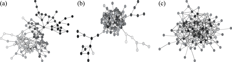
The topology optimization of a network of non-identical oscillators was also studied by Carareto et al. [342]. Their main goal was to obtain a complete synchronization with the smallest possible coupling strength $\lambda$. The authors verified that optimized networks exhibit strong anti-correlation between natural frequencies of adjacent oscillators, as in [336]. The verification that synchronization is enhanced when nodes are surrounded by neighbors of the opposite frequency was also observed for networks presenting symmetric bipolar distribution of natural frequencies [330]. Carareto et al. [342] also verified that this anti-correlation and degree homogeneity are not conflicting, proposing a solution for the heterogeneity paradox  [133].

Weighted networks were also studied in terms of optimization. Tanaka and Aoyagi [343] considered the Kuramoto model in weighted networks, i.e.,

$$\dot{\theta}_{i}=\omega_{i}+\sum_{i}A_{ij}w_{ij}\sin(\theta_{j}-\theta_{i}),$$ (342)

where $w_{ij}$ is the coupling strength between oscillators $i$ and $j$. The optimization was performed with respect to the coupling strength and natural frequency via assuming the constraint $\sum_{ij}\lambda_{ij}^{\alpha}=\lambda_{\mathrm{total}}^{\alpha}$, where $\alpha$ and $\lambda_{\mathrm{total}}$ are constants, and symmetric connections. By considering the steepest gradient of $r^{2}$, where $r$ is the order parameter, it was found theoretically update rules for the coupling strength and the natural frequency. Through the optimization procedure, they found that stronger weights are assigned to connections between pairs of oscillators with very different natural frequencies. The authors also verified that for a large $\lambda_{\mathrm{total}}$, the system of oscillators presents two natural frequencies, whereas for small $\lambda_{\mathrm{total}}$, there is a convergence of frequencies to one single value.

Several other papers further analyzed how the network organization can be adjusted to reach the optimal synchronization. The Kuramoto model with noise was addressed by Yanagita et al. [293]. Kelly and Gottwald [344] introduced an energy-like measure to quantify the correlation of frequencies with the same magnitude but opposite signs. They proposed an algorithm for minimization of this energy and, therefore, obtained optimized networks. The proposed method is computationally fast to generate optimized networks. Skardal et al. [345] derived a synchrony alignment function to measure synchronization, which can be used to optimize networks. They verified that synchronization is advanced by an alignment of the frequencies with the most dominant Laplacian eigenvectors. A matching between the heterogeneity of frequencies and network structure also improves the synchronization. Finally, we point out that optimization strategies considering external forcing were investigated in [346, 347, 348].

9 Applications

The Kuramoto model was firstly conceived with the aim to qualitatively explain how populations of oscillators fall into synchronization. However, since its formulation 40 years ago many real-world applications were reported, a fact that not even Kuramoto himself could foresee [349]. Now, his model has become relevant for the understanding of the dynamics of real complex systems which are internally organized into topologies way different than the regular ones long studied in theoretical physics. In this section we review some applications of the model in different fields, such as engineering, neuroscience, physics and even seismology. We should remark though that this is not about a comprehensive and complete review of real examples of synchronization, but rather about the description of recent applications of the Kuramoto model to real-world phenomena putting emphasis on the interplay between structure and dynamics. Regarding the former purpose we refer the reader to the classical texts in the field [1, 4, 14].

9.1 Power-grids

Power-grids, as one of the largest man-made networks, are a typical example to study collective behavior of networked elements, and its research has become increasingly important to its stability and network design for physicists and engineers [350, 304, 351, 352, 35, 353, 34, 354, 355, 356].

Consider an undirected and weighted AC power network, with $N$ generators and reduced admittance matrix $\mathbf{Y}$, at each generator $i$, the voltage phasor is accounted for by $V_{i}=|V_{i}|e^{i\theta_{i}}$ with the phase $\theta_{i}$ and magnitude $|V_{i}|$. Between connected generators $i$ and $j$, the allowed maximum power transferred is denoted by $\lambda_{ij}=|V_{i}||V_{j}|Y_{ij}$ as the coupling weight and the energy loss along the transmission is accounted for by $\varphi_{ij}$ with $\varphi_{ii}=0$. The governing dynamics as the network-reduced power system model at generator $i$ is given by [357, 352]

$$M_{i}\ddot{\theta}_{i}=-\alpha_{i}\dot{\theta}_{i}+\omega_{i}+\sum\limits^{N}_{j=1}\lambda_{ij}A_{ij}\sin(\theta_{j}-\theta_{i}+\varphi_{ij}),$$ (343)

where $M_{i}$ is the inertia coefficient, $\alpha_{i}$ is the damping coefficient, $\omega_{i}$ is the effective power input to $i$, and $\varphi_{ij}$ plays the role of phase shift. Figure 43 illustrates the network representation of a power-grid modelled by (343).

Figure 43: Illustration of the reduced model for power grid dynamics (Eq. 343) highlighting the two possible roles played by the nodes, namely as generators ($G$) or consumers ($C$).

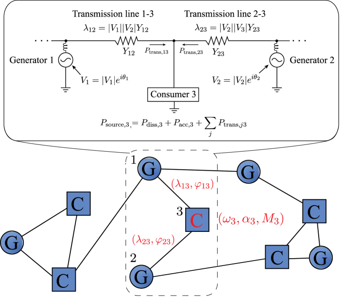
If the generator properties, voltage magnitudes and line reactances are assumed to be the same, and all lines are lossless, i.e. $\varphi_{ij}=0$, one can reproduce the original second-order dynamics (292). Let us review first the derivation of the model via simplifying the swing equation. To mimic essential properties of the nonlinear dynamics of a population of $N$ interconnected dynamical units in power grids, we consider a power grid model on coarse scales [299]. The state of each unit (machine) $i=1,\dots N$ is determined by its phase angle $\phi_{i}(t)$ and its velocity $d{\phi}_{i}(t)/dt$. Each unit rotates with the same frequency $\Omega=2\pi\times 50$ Hz or $\Omega=2\pi\times 60$ Hz, thus

$$\phi_{i}(t)=\Omega t+\theta_{i}(t),$$ (344)

where $\theta_{i}$ indicates the phase difference to the reference phase $\Omega t$.

During the rotation, the dissipated power is given by $P_{\mathrm{diss},i}=K_{D}(\dot{\phi}_{i})^{2},$ where $K_{D}$ is a friction coefficient. The kinetic energy follows $E_{\mathrm{kinetic},i}=I_{i}\dot{\phi}_{i}^{2}/2$ and the accumulated kinetic power is given by $P_{\mathrm{acc},i}=\frac{dE_{\mathrm{kinetic},i}}{dt},$ where $I_{i}$ is the moment of inertia. If a power flow between machines $i$ and $j$ exists, the power transmission is proportional to the sine of the phase difference, i.e. $\sin{(\phi_{j}-\phi_{i})}$ and the transmitted power follows $P_{\mathrm{trans},ij}=-P_{\mathrm{max},ij}\sin{(\phi_{j}-\phi_{i})},$ where $P_{\mathrm{max},ij}$ is the maximal capacity of the transmission line. If there is no power flow, $P_{\mathrm{trans},ij}=0$.

The power source $P_{\mathrm{source},i}$, which is fed into each machine $i$, has to be met by the sum of the power transmitted within the grid plus the accumulated and dissipated power, i.e., $P_{\mathrm{source},j}=P_{\mathrm{diss},j}+P_{\mathrm{acc},j}+\sum\limits^{N}_{i=1}P_{\mathrm{trans},ij}.$ Inserting Eq. 344 and the expressions of powers into the condition for energy conservation one gets [299, 358, 304]

$$I_{j}\Omega\ddot{\theta}_{j}=P_{\rm{source},j}-K_{D}\Omega^{2}-2K_{D}\Omega\dot{\theta}_{j}+\sum_{i=1}^{N}P_{\max,ij}\sin(\theta_{i}-\theta_{j}),$$ (345)

where it was assumed $|\dot{\phi}_{j}|\ll\Omega$ so that the terms $\dot{\theta}_{i}^{2}$ and $\dot{\theta}_{i}\ddot{\theta}_{j}$ can be neglected. For the sake of simplicity, considering that the moment of inertia $I_{i}$ and the line maximal capacity $P_{\mathrm{max},ij}$ are the same for all elements of the grid; defining $\omega_{j}\equiv(P_{\mathrm{source},j}-K_{D}\Omega^{2})/(I\Omega)$, $\alpha\equiv 2K_{D}/I$ and $\lambda_{ij}\equiv P_{\mathrm{max},ij}/(I\Omega)$, finally yields the original dynamics in Eq. (292) [299, 358, 304, 244] (Fig. 43). The power-grid model (343) with multiple time constants, nonhomogeneous coupling and nonuniform phase shifts was explored in [359].

The dynamics is simple enough to be analytically determined, yet sufficiently complex to exhibit various phenomena with insightful and comprehensive explanations. The bifurcation diagram of the one-node model is shown in Fig. 34 and that of a two-node subsystem consisting of one generator and one consumer shows quantitatively the same behavior. They all capture the essential feature of a real power grid, i.e., the coexistence of self-organized operation and power outage (see Sec. 7 of the second-order Kuramoto model). In this case, networks exhibit instability even without overloads [305].

In [352] a condition for synchronization on any arbitrary network was derived rigorously in terms of network topology and grid parameters . However, the model is based on simplifying (and unrealistic) assumptions, which makes its applications difficult. In order to fill this gap and further analyze more realistic networks, high-order models have been recently considered [360, 361, 362]. One of the issues pursued by these approaches is the precise understanding of effects of network structures on the collective behavior of power-grids. For instance, the British power-grid exhibits a bistable regime where normal operation and power outage coexist, as long as it contains a two-node topology [304] (see Sec. 7). The system could jump from self-organized synchronization to power outage under large perturbations. Further evidences were provided in various topologies, e.g., regular, random, and SW networks [363].

A possible source of perturbation that could cause power outrages is the temporary resetting of the values of power generation or consumption $\omega_{i}$, breaking the conservation condition and thus leading the system out of the synchronized state [350, 304, 351, 352, 35, 34, 354]. Futhermore, analyzing the single-node basin stability (see Sec. 7), it was found that, under the influence of even large perturbations, dead ends, dead trees and detour motifs play an important role in the grid stability [302, 331]. With respect to different nodes, basin stability as a function of the coupling strength was investigated, and it was found that the corresponding transition varies accordingly. In terms of the transition over an even large time window, nodes have a low community consistency, which yields that the basin stability transition is not sufficient to detect communities but is able to capture typical characteristics of individual nodes [356].

Cascading failures in the power supply are not only directly caused by large perturbations on single elements, but can also be induced by adding or removing links, e.g. the 2006 European blackout [364, 365, 366]. Interestingly, including new lines to a grid under normal operation does not always promote synchrony. In fact, it can potentially lead the network to operate incoherently and possibly induce power outages, a process that is similar to the Braess’s paradox in traffic networks [358]. Moreover, local overloads could be resulted by adding a remote link, which induces nonlocal failures [367].

Instead of adding links, a drastic change of electric power supply, the number of wind parks and other renewable energy sources could be increased, decentralizing generators and thus posing the question of how the self-organized synchronization and its stability would change correspondingly [304]. Combing renewable energy sources in the energy transition raises novel issues on the stability and design of power-grid networks. For instance, by replacing large centralized generators by small distributed ones, the number of crucial links, which if damaged desynchronizes the network, decreases, and therein more decentralized grids become more robust to topological failures [304]. In terms of dynamical perturbations, more decentralized grids become less robust [304]. Numerical simulations on various network topologies support that in decentralized grids, the system reaches its stable state for lower transmission line capacities, and thus decentralization favors power grids [363]. Effects of temporal energy feed-in fluctuations induced by renewable sources, e.g. solar plants [361], on synchronization and stability remain open. A rewiring algorithm by implementing a simple hill-climb method on switching edges was proposed to enhance synchronization [368]. Actually, given even that the network topology is fixed, localization of natural frequencies could affect synchronization. For example, in symmetric bipolar population networks, it was shown that synchronization is promoted when nodes are surrounded by nodes of different natural frequency [330] (see also Sec. 8).

Due to the increasing fraction of renewable energy sources, stable operation suffers from fluctuations of temporally evolving generations. To stabilize the normal operation, it was proposed to adapt generation via feedback control, termed as decentral smart grid control, where a local price is firstly determined by the local frequency as a function of time intervals and time delays, and then the frequency is varied according to this price [369]. The suggested control method promotes grid stability for, e.g., a sufficiently large averaging interval [369]. Additional to renewable sources, plug-in electric vehicles serve as distributed energy and increase power grid transient stability [370].

Various power-grid models could be derived depending on assumptions adopted for the generators equations (343), and the validity and appropriateness of them depend on specific purposes [371]. Taking into account that the electrodynamical behavior yields a third-order model with voltage dynamics (extended from the classical second-order Kuramoto model (292)), where the third characteristic, voltage, is included besides phase and frequency [361]. In comparison to the second-order Kuramoto model (292), this shows different stability behavior due to the evolution of voltage dynamics and should provide more realistic features of real power grids. Furthermore, considering voltage dynamics could yield even higher dimensional model [360]. For an overview of modern achievements and current open problems on the interdisciplinary research on power-grid dynamics we refer the reader to two recently published open issues [372, 373] and to the survey by Dörfler and Bullo [35], which offers an comprehensive review on applications of networks of phase oscillators to technological systems.

9.2 Neuronal networks

Synchronization phenomena play a prominent role in neuroscience. In fact, a plenty of evidences shows that synchronization is the key process through which information is processed in cortical areas of the brain [1, 374]. In particular, experiments in mammalian brains point out that different spatial patterns of synchronous firing are observed in the visual cortex when different visual stimuli are presented [374]. Further support for the hypothesis that collective behavior of groups of neurons is a general property of neuronal systems is found in the sensoriomotor cortex [375]. In this case, experiments show that synchronous oscillations emerge in field potential recordings with well defined frequencies whose amplitude and spatial coverage crucially depend on the motor task being executed [374, 375].

In order to better understand the underlying mechanisms that lead to neural synchronization, the neuroscience community has been invested great effort on the computational and theoretical study of neural- mass models coupled through structural substrates provided by neuroanatomical networks [376, 377, 378]. However, the analysis of highly accurate models in the physiologically point of a view can be rather challenging due to their complexity. On the other hand, in some situations, the models can be simplified to coupled phase oscillators akin to the Kuramoto model, which still yields a rich and non-trivial dynamics while being neurobiologically plausible [377]. For instance, Wilson-Cowan oscillators are generally used in the modeling neuronal dynamics of cortical regions  [379]. Using a phase reduction technique (see [380] for a recent review on phase reduction theory) one can show that the Wilson-Cowan model leads to a Kuramoto-like interaction. Furthermore, another feature that must be taken into account is that the oscillators are spatially embedded, a condition that inherently induces distance dependent coupling between the oscillators. These concepts were recently illustrated in [381], where the Wilson-Cowan model was shown, under the conditions that make the phase-reduction valid, to be equivalent to a Kuramoto model in a two-layered network subjected to time-delayed coupling. In this model, three macroscopic cortical dynamical states were found, namely incoherence (related to background activity), high synchronization (associated to epileptic behaviors) and also chaotic states, which turn out to be related to resting-state activities [381].

Neurons in the visual cortex respond accordingly to visual stimuli with different orientations. Thus, when a specific stimulus with a particular orientation is given, neurons that respond to the specific stimuli synchronize. Furthermore, evidences show that neurons in the fourth layer of the cortex have distance dependent connections with other neurons in a heterogeneous fashion [376]. These aspects of the neuron dynamics and the connectivity pattern of neurons in the visual cortex were taken altogether in [382], where the angle of synchronization of neurons was investigated by using Kuramoto oscillators coupled in SF networks embedded in 2D Euclidean spaces [383, 384]. Interestingly, despite its simplicity, the model was able to reproduce the emergence of clustered and stripped patterns akin to those ones observed in real experiments in infant macaques [385] and monkeys [386]. Moreover, by tuning the balance between inhibitory and excitatory couplings the model in [382] was even able to obtain patterns that qualitatively resemble experiments with ferrets [387].

Another utility of the Kuramoto model is to probe the topology of networks derived from neuronal data. As seen in Sec. 3, transient dynamics can reveal the underlying hierarchical organization of the network through the routes to synchronization [153, 157, 273, 388, 389, 390]. Such an approach was employed in the analysis of the cortical network of cats in [391], where it was verified that a synchronization transition between local and global states controlled by highly connected regions, such as the visual and auditory cortex, emerges. Interestingly, similar results as those ones got with the Kuramoto model in [391] can be obtained with models that encompass more sophisticated properties of neuronal dynamics. A similar strategy was carried out in [392] with the particular objective to characterize how lesions could affect the overall dynamics of the macaque cortical network. Lesions were modeled as perturbations on the synchronized and the impact of such disturbances was assessed by the time required for the nodes to return to the locked state. As shown in [392], the most robust nodes, i.e., the ones that presented shorter relaxation times, were reported to correspond to highly connected cortex areas, with the exception of the region V4, which turns out to be an intra-cluster hub. These results are in agreement with those presented in [29] regarding the relaxation time of nodes in SF networks. The effects of lesions in the local and global dynamics of cortical networks were further explored in [393], however with a different methodology. Specifically, instead of considering lesions in the cortex as random perturbations in the phases, the removal of nodes in the cortical network was adopted as such. In this case, the strongest impact in the networks’ global dynamics is achieved when nodes with higher eigenvector centrality are removed, inducing also metastability in the system [393].

Throughout this review, we saw the impact of different topological characteristics on synchronization mainly considering networks generated through random models (see especially Sec. 2 and 3). It is interesting to note that most of these findings were investigated in parallel in the neuroscience community by considering instead networks whose structure are derived from real data sets [394, 392, 391]. The questions posed in these studies are similar to those tackled among the physicists, e.g. the role played by hubs, communities, degree-degree correlations, etc; but with the aim of identifying the neurobiological importance of such properties. For instance, Schmidt et al. [394] investigated the potential role played by hubs in the brain dynamics by analysing the Kuramoto model in anatomical networks obtained through functional magnetic resonance (fMRI). One of the reported findings is that hubs have higher synchronization between themselves, a fact that is a consequence of high assortativity and modularity exhibited by these networks. Similar results were also observed for the Kuramoto model simulated on the macaque [392] and cat [391] cortical networks.

It is also important to mention the variation of the Kuramoto model analyzed by Cabral et al. [205] that incorporates heterogeneous time delay and stochastic fluctuations, i.e.:

$$\dot{\theta}_{i}=\omega_{i}+\lambda\sum_{j=1}^{N}A_{ij}\sin\left[\theta_{j}(t-\tau_{ij})-\theta_{i}(t)\right]+\xi_{i}(t),$$ (346)

where $\tau_{ij}$ is set to be proportional to the physical distance between nodes in the functional brain network. In  [205], the authors used the model in the gamma frequency range ($>30\rm{Hz}$) to generate time series to serve as input in the Balloon-Windkessel hemodynamic model [395]. Remarkably, the time series obtained through (346) were able to accurately describe the emergence of slow neural activity fluctuations empirically measured in real networks  [205]. Temporal and spatial synchronization patterns from fMRI were also reproduced for low frequencies between 0.01-0.13$\rm{Hz}$  [396], a range for which the time delays between the oscillators can be neglected, since the delay time scale in the cortex area is much faster than the periods of the oscillators [397]. Furthermore, the variant of the Kuramoto model (346) proved itself to be relevant in the study of criticality in brain dynamics  [398], besides also reproducing moment-to-moment fluctuations of phase differences of resting states in magnetoencephalography (MEG) oscillations recorded during finger movement experiments  [399]. Other aspects of dynamical criticality in human brain functional networks were studied in [400] by comparing times series generated with the Kuramoto model and fMRI data recorded from normal subjects under resting conditions.

Other recent works have investigated further aspects of the relation between structure and dynamics of phase oscillators in anatomical and functional cortical networks [401, 402, 403, 404, 378, 405, 406, 214], which includes studies on the effects of remote synchronization [407, 408, 409], a toolbox for large-scale simulations of brain dynamics using different models [410] and discussions about the limitations of the above mentioned approaches [411].

9.3 Networks of disordered Josephson junctions

A locally coupled Kuramoto model with a second-order time derivative (LKM2) can be derived from a coupled resistively and capacitively shunted junction equations (RCSJ) for an underdamped ladder with periodic boundary conditions [298]. Phase synchronizations on these two models are investigated in terms of the Kuramoto order parameter and the degree of frequency synchronization defined as

$$f=1-\frac{s_{V}(\lambda)}{s_{V}(0)},$$ (347)

where $s_{\nu}(\lambda)$ denotes the standard derivation of the $N$ time-average voltage $\left\langle V_{i}\right\rangle$ as a function of the coupling strength $\lambda$ as follows

$$s_{V}(\lambda)=\sqrt{\frac{\sum^{N}_{i=1}\left[\left\langle V_{i}\right\rangle-(1/N)\sum^{N}_{j=1}\left\langle V_{j}\right\rangle\right]^{2}}{N-1}}.$$ (348)

When $f=1$ all $N$ junctions’ frequencies are signaled and $f=0$ when neighboring rung junctions are uncoupled. In the absence of any coupling i.e. $\lambda=0$, phase value of each junction follows

$$\phi_{i}(t)=A+Be^{-\tau/\beta_{c}}+\omega_{i}\tau,$$ (349)

where $\tau$ is dimensionless time unit given by $\tau=2e\left\langle I_{c}\right\rangle/\hbar\left\langle R^{-1}\right\rangle$, with $\left\langle I_{c}\right\rangle$ the average critical current and $\left\langle R\right\rangle$ the average resistance. Moreover, $\beta_{c}$ is the McCumber parameter given by $\beta_{c}=2e\left\langle I_{c}\right\rangle\left\langle C\right\rangle/\hbar\left\langle C\right\rangle^{2}$, where $\left\langle C\right\rangle$ is the average capacitance of the system. $A$ and $B$ are constants that depend on the initial conditions. In the uncoupled limit we have $d\phi_{i}/d\tau=\omega_{i}$, thus $\omega_{i}$ can be regarded as the voltage across junction $i$ in the uncoupled regime.

Good agreements between LKM2 and RCSJ are achieved for phase synchronization as well as frequency synchronization, but the LKM2 is easier to be solved and understood compared to the RCSJ [298]. On SW networks, shortcut links enhance synchronization on ladder arrays, but in two-dimensional arrays, the effects on synchronization are marginally restricted [298].

9.4 Seismology

An interesting and promising recent application of the Kuramoto model comes from the modeling of earthquakes. Scholz [412] was the first to postulate that the Kuramoto model can be applicable to explain the sequencing of nearby faults after a large earthquake. This is supported by the hypothesis that a seismically active fault can be regarded as a limit cycle relaxation oscillator. Specifically, when a given fault on the earth’s crust accumulates stress until a certain threshold an earthquake occurs, which reduces the stress in this particular fault and, at the same time, distributes the energy released contributing to increase the stress in the nearby faults and then triggering new events [412]. Although this process resembles a pulse-coupled dynamics, many insights can be gained from the study of phase oscillators. However, considering synchronization of faults in a globally coupled topology seems quite unrealistic, since the spread of energy is made through local fault-fault interactions, making the network approach to the problem much more suitable. In order to model this process, Vasudevan et al. [413] considered a directed network constructed from the sequencing of earthquake events provided by the Incorporated Institutions for Seismology (IRIS) for the time span between 1970 and 2014. In this network, each node corresponds to an earthquake event and a directed edge departing from node $i$ and reaching node $j$ exists if earthquake $i$ triggered another one in node $j$. Furthermore, the phases of the model were considered to evolve according to [413]

$$\dot{\theta}_{i}=\omega_{0}+\lambda\sum_{j=1}^{N}e^{-\kappa d_{ij}}\sin(\theta_{j}-\theta_{i}+\varphi),$$ (350)

where $\varphi$ accounts for the non-instantaneous energy transmission, $d_{ij}$ is the shortest path length between two fault points $i$ and $j$ in the earthquake events grid and $\kappa$ is the strength of the non-local coupling. Interestingly, it was found that the dynamics in the earthquake network supports the occurrence of chimera states, which might be a result from the interplay between phase-lag interaction and the geodetic constraints in the earthquake zones [413]. The study of sequencing of earthquakes using phase models is still in its infancy and much remains to be explored, specially concerning the investigation of effects of other parameters in the model, such as heterogeneity in the natural frequencies and the inclusion of heterogeneous time-delays between the oscillators. Another promising direction is the consideration of other models that incorporate excitable behavior, e.g. the Shinomoto-Kuramoto model (see Sec. 6).

Finally, we would like to mention that the Kuramoto model in complex networks has been considered in many other applications, such as machine learning [414, 415, 416, 417, 418, 419], characterization of financial market networks [420], modelling of groups of animals in motion [421], oscillatory dynamics of cell networks [422], logistics [423, 424, 425] and opinion dynamics [426, 427, 428], besides being employed in the methods for community detection in networks based on phase oscillators discussed in Sec. 3.3.

10 Conclusions and perspectives

In this article we have reviewed recent advances in the study of Kuramoto oscillators in complex networks. We have focused our analysis on how the local and global dynamics are influenced by the network connectivity pattern. As we saw, in the last years, the Kuramoto model has been scrutinized and many different scenarios were considered since the first works addressing synchronization in networks were published. Here we sum up these contributions and commenting what are most interesting and promising open problems for future research.

We started by analysing the dynamics in standard network models (Sec. 2), i.e. SW, random and SF topologies; which were the subject of the early works that established the foundations for many further studies. In particular, we presented necessary approximations to treat the problem, including the most employed MFA. Interestingly, although being unquestionably seminal contributions, it was evident that the first works investigating the Kuramoto model in complex networks were surrounded by questions that the inclusion of the heterogeneous connections had raised. Some of these questions, unfortunately, still remain without an answer. In particular, the disagreement between the finite value observed in simulations and the prediction of a vanishing critical coupling for the onset of synchronization by the MFA in SF networks is one of the most challenging puzzles that persisted from the early investigations. However, despite the fact that Kuramoto oscillators have long been studied in these traditional topologies, there are also recent fundamental new results on the dependence on the system size and on the relaxation dynamics of the model. In the former topic, we showed the importance of considering sample-sample fluctuations for the correct estimation of the scaling exponents. Regarding the relaxation dynamics, we saw the non-intuitive phenomenon of requiring larger relaxation times to reach the stationary state in the SW regime. This is a surprising effect giving the many results by previous studies showing that synchronization is attainable for weaker couplings in comparison to regular topologies. It is worth mentioning that the study of the time-dependent dynamics was also greatly benefited thanks to the Ott-Antonsen theory, whose application was exemplified in the study of the relaxation dynamics of SF networks.

In Sec. 3 we moved one step further in the level of topological description of networks by introducing a new set of structural features that are absent in uncorrelated ones. More specifically, we analyzed synchronization of Kuramoto oscillators in network models that mimic, to some extent, connectivity patterns which are often encountered in real-world networks, such as clustering, modular organization and degree-degree correlations. Initial numerical investigations exhibited that the increasing of clustering has a negative effect on the network synchronization. In other words, networks with a high occurrence of triangles reach lower levels of synchronization in comparison with networks with the same degree distribution at the some coupling strength. However, as we have discussed, as the clustering is increased when employing stochastic rewiring algorithms, several other properties in the network are changed, even though the degree distribution remains fixed. The alternative approach is then to consider the aforementioned models, which, besides being able to generate particular topological properties of interest, further allow analytical tractability. Possibly here lies one of the most fruitful directions to be explored in future works, i.e. the development of analytical techniques that go beyond the MFAs for locally tree-like networks.

After investigating the effects of structural properties of real systems on network dynamics, in Sec. 4 we reviewed effects of dynamical features that provide a more realistic modelling of special classes of systems. Specifically, we studied effects of time-delayed couplings, which are present in the synchronization of systems in which the speed of signal transmission is comparable to oscillators’ periods, and scenarios where the couplings (and the network structure) is time-dependent. Regarding the former, we observed that the dynamics is significantly changed compared to the case where the interaction is instantaneous. In particular, new dynamical states were observed to emerge. However, while the impact of delay on synchronization is well understood in small populations, there is still a lack of results on the time-delayed dynamics of large heterogeneous networks. There are interesting topics for new research in this direction, such as progress can be achieved by applying the OA theory in networks in order to thoroughly evaluate the influence of delay on the dynamics as well as the relation with the network structure. The same is valid for research on adaptive topologies. This is one of the branches in the research of the Kuramoto model in networks that is in its infancy and much remains to be done.

Section 5 reviewed one of the most active topics in the last years within the research of phase oscillators in networks: the correlation between natural frequencies and degrees. This strategy to assign frequencies to the network yielded the first report of discontinuous synchronization phase transitions in SF networks and, consequently, attracted the attention of many researchers. However, as later shown, this particular mechanism turned out to be not the only one to lead to such an abrupt emergence of collective behavior in networks. The key point is the existence of a sufficiently large gap between the natural frequencies of connected nodes, a condition that is automatically satisfied in SF networks if $\omega_{i}\sim k_{i}$. The effect of other correlations between intrinsic dynamical characteristics and local topological properties could be an interesting topic for future research.

Section 6 addressed the Kuramoto model in networks in the presence of noise. Intriguingly, despite the popularity of the model in the last decade, its stochastic version still has many scenarios to be explored. For instance, we presented the derivation of the nonlinear Fokker-Planck equation and thereby obtained the onset of synchronization. However, a quantitative analysis of the interplay between the stochastic dynamics and the structure of SF was still not tackled. In particular, it would be interesting to combine the approaches developed in Sec. 6 and those in Sec. 2.2 in order to explicitly determine the dependence with the system size. Another interesting direction is to analyze how the relaxation time in networks is affected by stochastic forces. For this task, the OA ansatz used to uncover the temporal dynamics (see Sec. 2.3) is no longer applicable. Conversely, as shown in Sec. 6.2, a dimension reduction is still possible through a Gaussian approximation, which has been recently providing insightful results into the time dependent behavior of the stochastic Kuramoto and Shinomoto-Kuramoto model [282, 86, 87, 429]. Regarding the latter, we saw that interesting phenomena can arise in the excitable dynamics as a consequence of the inclusion of heterogeneous connectivity patterns. Other scenarios are naturally appealing to consider in future studies, such as the inclusion of delay and degree-degree correlations. In particular, it would be interesting, for instance, to verify whether the transitions between periodic and quasiperiodic states induced by degree correlations [96] and chaos generated by frequency correlations [144] still persist in the presence of noise. Moreover, the stochastic Kuramoto model subjected to attractive and repulsive couplings [429, 430, 431, 432, 433, 434] could possibly reveal further peculiarities in the dynamics in networks.

In Sec. 7 we have reviewed studies on the second-order Kuramoto model. Such a variation of the original model was firstly conceived in order to encompass frequency adaptation, a property observed in synchronization of biological rhythms, such as exhibited by fireflies and circadian rhythms. We started by first providing a brief overview of the recent developments on the model in the fully connected graph with and without the influence of stochastic fluctuations. We followed up by considering the model in uncorrelated networks, where the mean-field treatment presented in Sec. 2.1 was applied to the case with inertia. Despite the progress achieved in the last years in understanding the effects of inertia [4], the theory discussed still has some fundamental limitations. For instance, in order to obtain the synchronization conditions for locked oscillators we assumed sufficiently small values for the damping coefficient so that Melnikov’s method can be applied. For large values of mass and damping the approximations are no longer valid and results to fill this gap are still missing. Furthermore, the stochastic Kuramoto model with inertia in networks also remains largely unexplored. An interesting approach to tackle this problem would be to consider dimension reduction techniques such as the Gaussian approximation in Sec. 6.2 or even the one recently introduced in [435]. It is also worth mentioning that the second-order Kuramoto model was brought to higher attention lately partially due to recent interest in the synchronization of power grid systems. We strongly believe that this branch in the field of network synchronization will develop even further. In particular, much effort has been put into the characterization of the stability of such systems using new set of complexity measures. For instance, the aforementioned basin stability has been successfully applied to quantify the robustness of power-grid networks against large perturbations to the synchronized state.

Methods to optimize synchronization were examined in Sec. 8. Here the main question addressed is which type of topology or frequency assignment maximizes the collective behavior among the oscillators given certain constraints. This topic is particular appealing for various applications, since typically the design of real systems is surrounded by constrains that arise due to a limited amount of resources. In this regard, much can be learned from investigations presented in Sec. 8. Moreover, studies on optimization of any kind of dynamics in networks heavily rely on expensive computational tasks. However, interesting analytical approaches have been taken concerning optimization of networks consisting of Kuramoto oscillators [345, 435, 436]. Interestingly, the study of optimal frequency assignments can be benefited from the results discussed in Sec. 5, since the correlation between frequencies and degrees has been reported to provide an optimal scenario for the emergence of synchronization. In the light of these results, it is therefore very likely that more work will attempt to better understand conditions which significantly improve network synchronization.

Section 9 is devoted to review some applications of the Kuramoto model in real systems. There we discussed how insights gained in the long studied question of how topology shapes dynamics (and vice-versa) have been put into practice. For instance, thanks to the joint approach of network characterization and application of non-linear stability measurements, important findings were obtained regarding the dynamics of real power-grid networks. In particular, the contribution of particular types of subgraphs to the overall grid’s stability was assessed through the new concept of basin stability, whereby the non-intuitive phenomenon that stability is threatened by dead-ends and dead-trees in the topology was uncovered. These findings allied with extensions to higher-order power-grid models have great potential to become guidelines in the development of new policies in power-grid design and management. Furthermore, it is becoming clear that, despite its simplicity, the Kuramoto model plays an important role in the characterization and modelling of the dynamics in cortical networks. Understanding the neuronal dynamics in networks obtained from real data using the model variations discussed in Sec. 9 can potentially pave the way for studies with more sophisticated models. These and other examples showed in Sec. 9 along all the results reported in this paper might also motivate applications of the Kuramoto model in other fields.

The relation between dynamics and structure of the Kuramoto model in complex networks was scrutinized over the last years. Much has been done since the first works addressing synchronization in networks came out. However, there are still many gaps to be filled and other scenarios to be explored. The combinations of different topologies and variations of the model dynamics are countless. Furthermore, the myriad of works published in the last decade on synchronization of phase oscillators in networks, as well as other dynamical processes, was a natural consequence of the growing interest in trying to understand the topological organization of real complex systems. Nowadays, we observe an analogous movement that aims at characterizing the structure of multilayer networks, a fact that makes us to expect a huge number of works devoted to the analysis of dynamical processes in these structures.

Finally, we believe that the present review complements previous works offering a guide on structural aspects of the dynamics of Kuramoto oscillators for new researchers in the field.

11 Acknowledgements

We are indebted with B. Sonnenschein, E. R. dos Santos, P. Schultz, C. Grabow, M. Ha and C. Choi for insightful and helpful discussions. T.P. acknowledges FAPESP (No. 2012/22160-7 and No. 2015/02486-3) and IRTG 1740. P.J. thanks founding from the China Scholarship Council (CSC). F.A.R. acknowledges CNPq (Grant No. 305940/2010-4) and FAPESP (Grant No. 2013/26416-9). J.K. would like to acknowledge IRTG 1740 (DFG and FAPESP).

Appendix A Complex Networks

The structure of complex network can be represented by a graph $G$ composed of an ordered pair of disjoint sets $G=(V,E)$, where $V$ is a set of elements called vertices (nodes) and $E$ is a subset of ordered pairs of distinct elements of $V$, called edges [8, 10]. If the network is directed, then the connections are called arcs (or directed links). While a protein-protein interaction network is undirected, a network of neuronal connections is typically directed [15]. Mathematically, the organization of networks can be represented by the adjacency matrix $\mathbf{A}$, whose elements $A_{ij}=1$ if there is a connection between nodes $i$ and $j$ or $A_{ij}=0$ otherwise. In undirected networks, $\mathbf{A}$ is symmetric, whereas for directed networks, $\mathbf{A}$ is generally asymmetric. Figure 44 illustrates the mapping of a network in the respective adjacency matrix for the directed and undirected cases.

The organization of networks can be characterized by network measures [12]. The node degree $k_{i}$, which represents the number of edges connected to node $i$, is one of the most simple measures for local network characterization. For undirected networks it can be calculated as

$$k_{i}=\sum_{j}A_{ij}=\sum_{j}A_{ji}.$$ (351)

For instance, in Figure 44(a), we have $k_{2}=1$, $k_{1}=k_{4}=k_{6}=2$, $k_{3}=3$ and $k_{5}=4$.

The density of connections in a network can be quantified by its average degree, which is calculated by

$$\langle k\rangle=\frac{1}{N}\sum_{i}k_{i}=\frac{1}{N}\sum_{ij}A_{ij}.$$ (352)

Figure 44: Graphs can be represented by adjacency matrices. In (a) we have a example of a undirected graph and (b) a directed graph. In (a), the matrix elements $A_{ij}=1$ if there is a connection between the nodes $i$ and $j$ or $A_{ij}=0$ otherwise. In (b), the matrix elements $A_{ij}=1$ if there is a directed connection (an arc) from node $i$ to node $j$.

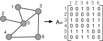
In the case of directed networks, in which the connections have directions, a node can be characterized by the out-degree, $k_{i}^{\mathrm{out}}$, which yields the number of outgoing edges, and the in-degree, $k_{i}^{\mathrm{in}}$, corresponding to the number of incoming edges [25]. In terms of the adjacency matrix, we have

$$k_{i}^{\mathrm{out}} = \sum_{j}A_{ij},$$ (353)

$$k_{i}^{\mathrm{in}} = \sum_{j}A_{ji}.$$ (354)

For instance, in Figure 44(b), $k_{1}^{\mathrm{in}}=1$ and $k_{1}^{\mathrm{out}}=2$. The total degree of a node $i$ is defined as $k_{i}=k_{i}^{\mathrm{in}}+k_{i}^{\mathrm{out}}$.

In unweighted networks, the connections are binary, i.e., $A_{ij}=1$ or $0$, indicating the presence or absence of an edge. However, some networks have weighted connections, which can indicates the strength of the interactions between pairs of nodes [437]. For a road network, for instance, the weight can specify the inverse of the distance between pairs of cities. Therefore, the closer two cities, the higher the strength of their interconnection. A weighted network can be completely represented in terms of its weight matrix $\mathbf{W}$, so that each element $W_{ij}$ expresses the weight of the connection from vertex $i$ to vertex $j$. In addition, instead of the node degree, we use the node strength of $i$, $s_{i}$, which is defined as the sum of the weights of the corresponding edges [437]. In terms of the weight matrix, for an directed and weighted network, the in and out-strength is defined as [437]

$$s^{\mathrm{out}}_{i} = \sum_{j}W_{ij},$$ (355)

$$s^{\mathrm{in}}_{i} = \sum_{j}W_{ji}.$$ (356)

By using the concept of degree, it is possible to characterize the large-scale network organization by considering the degree distribution $P(k)$, which yields the probability that a node selected randomly presents the degree $k$. The second statistical moment of $P(k)$ quantifies the network level of heterogeneity and is related to several dynamical processed running on the top of complex networks [11]. Particularly, the critical coupling of the Kuramoto model depends inversely on the second moment of $P(k)$ [60].

Networks whose degree distribution follows a power-law (or Pareto distribution [438]) are called scale-free networks [10], i.e.,

$$P(k)\sim k^{-\gamma},$$ (357)

implying that the degree distribution appears as a straight line when plotted on a loglog graph. Such networks are characterized by an inhomogeneous topological organization, where most of the nodes present a small number of connections, whereas a small fraction of nodes is densely connected. These densely connected nodes, called hubs, play a fundamental role in the topology and dynamics of complex networks.

Another fundamental concept in networks is related to distances, such as the number of edges along the path connecting two vertices [12]. There are many important topological and dynamical properties related to distances, such as random walks, which are defined by any sequence of adjacent nodes. A path is a special type of walk, which does not allow repetition of nodes or edges. The paths with the minimum length between two nodes $i$ and $j$ are called the shortest paths [12]. Observe that it is possible to have more than one path with the shortest length connecting two nodes. This length, which is called geodesic distance, is henceforth represented as $d_{ij}$. Thus, it is possible to characterize the large scale organization of a network by averaging the geodesic distances between every pair of nodes. The average shortest path length is defined by

$$\ell=\frac{1}{N(N-1)}\sum_{i\neq j}d_{ij}.$$ (358)

Observe that this definition has a limitation, since the value of $\ell$ diverges if two nodes do not belong to the same component, which yields $d_{ij}=\infty$. A possible approach to avoid this divergence is to consider only the nodes in the largest component while calculating the value of $\ell$.

Networks can also be characterized in terms of the presence of triangles (subgraphs composed by three fully connnected nodes) [8]. The fraction of triangles can be determined by a measurement called transitivity (or global clustering coefficient). Transitivity measures the probability that the adjacent neighbors of a vertex are connected. For undirected unweighted networks, the transitivity is calculated as [8, 25, 12]

$$\mathcal{T}=\frac{3N_{\triangle}}{N_{3}},$$ (359)

where $N_{\triangle}$ corresponds to the number of triangles observed in a network and $N_{3}$ is the number of connected triples. Fig. 45 illustrates the concepts of triangles and connected triples. The factor three in this equation is due to the fact that each triangle consists of three different connected triples, one with each of the vertices as central vertex, which assures that $0\leq\mathcal{T}\leq 1$. By using the adjacency matrix, these properties can be calculated as

$$N_{\triangle}=\sum_{k>j}^{N}\sum_{j>i}^{N}\sum_{i=1}^{N}A_{ij}A_{ik}A_{jk},$$ (360)

$$N_{3}=\sum_{k>j}^{N}\sum_{j>i}^{N}\sum_{i=1}^{N}(A_{ij}A_{ik}+A_{ji}A_{jk}+A_{ki}A_{kj}).$$ (361)

Figure 45: Illustration of the definition of transitivity. This network presents one triangle and eight connected triples (three of these triples are indicated by gray arrows). Therefore, in this network, we have $\mathcal{T}=3/8.$

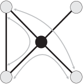
$\mathcal{T}$ is a measure for large scale network characterization. However, it is possible to define the local clustering coefficient of a node $i$, which quantifies how well the immediate neighbors of that node are interrelated [74]. More specifically, the clustering coefficient is defined as

$$cc_{i}=\frac{2e_{i}}{k_{i}(k_{i}-1)},$$ (362)

where $e(i)$ is the total number of undirected edges interconnecting the immediate neighbors of $i$. Notice that $0\leq cc(i)\leq 1$. The number of edges among the neighbors of a node $i$ can be calculated by

$$e_{i}=\frac{1}{2}\sum_{j=1}^{N}\sum_{k=1}^{N}A_{ij}A_{jk}A_{ki}.$$ (363)

Figure 46 illustrates the calculation of the clustering coefficient.

Networks can also be characterized in term of degree-degree correlations [439], which can be analyzed in terms of the conditional probability $P(K^{\prime}=k^{\prime}|K=k)=P(k^{\prime}|k)$, i.e., the probability that a vertex of degree $k$ is connected with a vertex of degree $k^{\prime}$. In uncorrelated networks, $P(k^{\prime}|k)$ does not depends on $k$ and the only relevant function for networks characterization is $P(k)$ [439]. However, due to the difficulties in estimating the conditional probability of degree-degree connectivity in empirical data [25], researchers often use the assortativity coefficient $\mathcal{A}$ as a measure of degree-degree correlation. The correlation between a pair of random variables is calculated by taking into account the Pearson correlation coefficient. Thus, it is natural to recur to this approach to determine the correlations in networks [8], i.e.,

$$\mathcal{A}=\frac{\frac{1}{|E|}\sum_{j>i}k_{i}k_{j}A_{ij}-\left[\frac{1}{|E|}\sum_{j>i}\frac{1}{2}(k_{i}+k_{j})A_{ij}\right]^{2}}{\frac{1}{|E|}\sum_{j>i}\frac{1}{2}(k_{i}^{2}+k_{j}^{2})A_{ij}-\left[\frac{1}{|E|}\sum_{j>i}\frac{1}{2}(k_{i}+k_{j})A_{ij}\right]^{2}},$$ (364)

where $|E|$ is the number of edges. Note that $-1\leq\mathcal{A}\leq 1$. In the case of $\mathcal{A}>0$, vertices with similar degrees tend to connect with each other and the network is classified as assortative. On the other hand, if $\mathcal{A}<0$, vertices with high degree tend to connect with low degree nodes, or vice versa, and the network is called disassortative. If $\mathcal{A}=0$ there is no correlation between the degrees.

Figure 46: Examples of clustering coefficient calculated for the (central) red node.

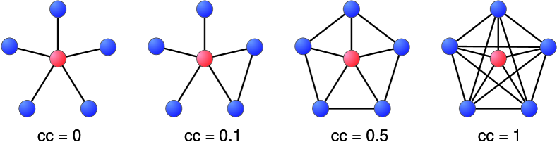
Centrality is a node property that can influence the network synchronization (e.g. [440]). Although centrality is important for node characterization, there is no single definition of centrality in a complex network [441]. For instance, the concept of “centrality” can be related to the average shortest distances [147], network spectra [442] and random walks [443]. A possible measure is given by the betweenness centrality [147], i.e.,

$$b_{u}=\sum_{ij}\frac{\sigma(i,u,j)}{\sigma(i,j)},$$ (365)

where $\sigma(i,u,j)$ is the number of shortest paths between vertices $i$ and $j$ that pass through vertex (or edge) $u$, $\sigma(i,j)$ is the total number of shortest paths between $i$ and $j$, and the sum is over all pairs $i,j$ of distinct vertices. Thus, a central node in a network should be crossed by many paths and therefore present a high value of betweenness centrality. This property can be verified in a city, as its nodes at center tend to present the highest traffic, i.e. to go from a region to another, it is necessary to pass through the center of the city. $b_{u}$ plays a fundamental role on network synchronization [440].

In addition to the degree-degree correlation, presence of triangles and heterogeneous structure, complex networks may display modular organization [147, 146]. The modules are groups whose vertices are more densely interconnected one another than with the rest of the network. These modules are called communities in network theory. Many networks present community organization [146], e.g. social sciences, families, friendship circles, co-workers, scientific collaborations and villages are examples of communities. In the World Wide Web, pages related to the same or related topics tend to be connected, forming communities.

There are several methods to find communities in networks [146]. To quantify the quality of a particular division, most methods have adopted the modularity measure [159]. This measurement is based on the comparison between the fraction of the edges that fall within the communities and the expected fraction whether edges were distributed at random. Mathematically,

$$Q=\frac{1}{2M}\sum_{i=1}^{N}\sum_{j=1}^{N}\left(A_{ij}-\frac{k_{i}k_{j}}{2M}\right)\delta(C_{i},C_{j}),$$ (366)

where $\delta(C_{i},C_{j})$ is the Kronecker delta, which is equal to one if $C_{i}=C_{j}$ and zero, otherwise. The term $(k_{i}k_{j})/2E$ represents the expected number of edges between the vertices $i$ and $j$ in the configuration model. The best network division in communities yields the largest value of modularity.

Several other measures can be considered for networks characterization [12]. They are used to understand the relation between networks structure and synchronization.

A.1 Complex networks models

Complex systems exhibit specific types of organization resulting from intrinsic rules and constraints that guide the system’s evolution, e.g. the interconnection between components in power grids (whose nodes are power stations, transmission circuits, and substations) is to a great extent a consequence of the geographical distance between nodes [444]. In other words, two geographically close nodes tend to be connected, while distant nodes are not likely to connect. Therefore, the degree distribution of this type of network depends on the geographical node distribution [444]. For instance, if the distribution of nodes is uniform in the two-dimensional space, it is expected that the degree distribution will be close to a Poisson distribution. On the other hand, in collaboration networks, composed by scientists connected according to coauthorships of scientific works, the most connected researchers tend to attract more scientists for collaborations (knwon as the rich get richer paradigm). In this case, the degree distribution follows a power law.

Since different rules result in different topologies, some basic models have been proposed to generate networks with a given degree distribution and other topological properties. These models are fundamental to generate networks in which it is possible to control some properties, such as $\left\langle k\right\rangle$ and $\mathcal{T}$. As following, we present the most famous models of complex networks.

A.1.1 Random Graphs

A simple stochastic model for the generation of random graphs was proposed by the mathematicians Paul Erdős and Alfred Rényi in 1959 [445]. A random graph (ER) is generated by starting with $N$ disconnected nodes and then connecting each pair of nodes according to a fixed probability $p$. Therefore, this process is a type of $N^{2}$ realization of a Bernoulli process with probability of success $p$. Therefore, the number of connections follows a binomial distribution. Nevertheless, as most realizations of this model take into account large values of $N$ and small values of $p$, the degree distribution tends to a Poisson distribution (known as the law of rare events). For small $p$ and large $N$, we have

$$P(k)=\frac{N!}{(N-k)!k!}p^{k}(1-p)^{k}\simeq\frac{e^{-\langle k\rangle}\langle k\rangle^{k}}{k!},$$ (367)

where $\langle k\rangle=p(N-1)$ is the average degree of the network. Random graphs exhibit a second order percolation phase transition according $\left\langle k\right\rangle$. If $\langle k\rangle>1$, there is an emergence of a giant component [446].

A.1.2 Small-world networks

The ER network is not suitable to model the vast majority of real-world systems. Indeed, it is difficult to find a system whose structure is similar to ER. In this way, in order to generate networks with a more structured topology, Watts and Strogatz suggested a model whose structure lies between a complete regular graph and a random network [74]. The Watts-Strogatz small-world model (SW) generates networks with a large number of loops of size three, i.e. three nodes connected to each other (a loop). This property is observed in cohesive networks, such as in society, where two friends $A$ and $B$ present a high probability to share a common friend $C$, as quantified by the clustering coefficient (Eq. 362).

In order to construct a SW network, one starts with a ring of $N$ vertices, in wihch each vertex is connected to $\kappa$ nearest neighbors in each direction, totalizing $2\kappa$ connections. Next, we choose a vertex and the edge to its nearest clockwise neighbour. With probability $p$, this edge is reconnected to a vertex chosen uniformly at random over the entire ring. This process is repeated by moving clockwise around the ring, considering each vertex at time until one lap is completed. When $p=0$ we have an ordered lattice with clustering coefficient, but with long average shortest paths. When $p\rightarrow 1$, the network becomes a random graph with small shortest distances between nodes but few loops. Notice that for $p=1$ a network does not become an ER network. Figure 47 presents SW networks generated with different values of the probability $p$.

Figure 47: Small-world networks composed by $N=20$ vertices and $\left\langle k\right\rangle=3$. Different rewiring probabilities $p$ are taken into account.

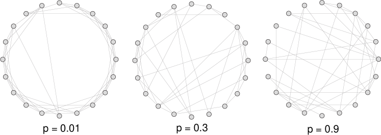
A.1.3 Scale-free networks

The model of Watts and Strogatz overcomes the lack of structure present in random graphs while providing an elegant theory to explain the presence of cycles of order three, as well as the dependence between the average shortest path and the network size. However, since this model does not generate networks with power-law degree distribution, it is not suitable to represent many real-world networks, such as the Internet, biological networks and World Wide Web [15]. In 1999, Barabási and Albert [5] proposed a simple algorithm to construct networks, whose degree distribution follows a power-law. This model, known as SF Barabási-Albert model (BA), is based on two principles: (i) growth and (ii) preferential attachment. The network is generated starting with a set of $m_{0}$ connected vertices; afterwards, at each step of the construction the network grows with the addition of a new vertex. For each new vertex, $m$ new edges are inserted between the new vertex and some previous vertex. The vertices which receive the new edges are chosen following a linear preferential attachment rule, i.e. the probability of the new vertex $i$ to connect with an existing vertex $j$ is proportional to the degree of $j$,

$$\mathcal{P}(i\rightarrow j)=\frac{k_{j}}{\sum_{n}k_{n}}.$$ (368)

This rule indicates that the most connected nodes present a high probability to receive new connections.

A.1.4 Configuration model

Figure 48: Illustration of the configuration model. Stubs are selected uniformly and connected, forming a network with a defined degree sequence. Dashed lines indicate the connections between pairs of stubs.

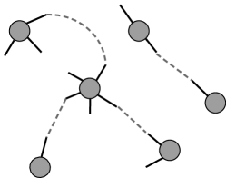
ER, SW and BA models generate networks with a well defined degree distribution. However, in some cases, the degree distribution of real-world networks is not homogeneous and the coefficient of the power law is not the same as that observed in the BA model. Therefore, it is important to have a model that enables the construction of a network with an arbitrary degree distribution, while preserving the other network properties as random.

The configuration model is a model of random graph with a defined degree sequence $\bm{k}=\{k_{1},k_{2},\ldots,k_{n}\}$ [97, 98, 447], where $k_{i}$ represents the number of connections of node $i$. To construct the network, initially, each node $i$ receives a total of $k_{i}$ stubs (half edges). Then, at each time step, two stubs (half-edges) selected uniformly are connected. This process is repeated until all stubs are connected. In Figure 48 we can see an illustration of the configuration model algorithm. Notice that self-loops and multi-edges are allowed in this model. At the end of the process, we have a network with a defined degree distribution.

References

- [1] A. Pikovsky, M. Rosenblum, J. Kurths, Synchronization: a universal concept in nonlinear sciences, Vol. 12, Cambridge University Press, 2003.
- [2] Y. Kuramoto, "Self-entrainment of a population of coupled non-linear oscillators." International symposium on mathematical problems in theoretical physics. Springer Berlin/Heidelberg, 1975. NBR 6023.
- [3] Y. Kuramoto, Chemical Oscillations, Waves, and Turbulence, Springer, Berlin, 1984.
- [4] J. A. Acebrón, L. L. Bonilla, C. J. P. Vicente, F. Ritort, R. Spigler, The Kuramoto model: A simple paradigm for synchronization phenomena, Reviews of modern physics 77 (1) (2005) 137.
- [5] A.-L. Barabási, R. Albert, Emergence of scaling in random networks, science 286 (5439) (1999) 509–512.
- [6] A.-L. Barabási, The network takeover, Nature Physics 8 (1) (2011) 14.
- [7] G. Bianconi, Interdisciplinary and physics challenges of network theory, EPL (Europhysics Letters) 111 (5) (2015) 56001.
- [8] M. E. J. Newman, The structure and function of complex networks, SIAM review 45 (2) (2003) 167–256.
- [9] S. N. Dorogovtsev, J. F. Mendes, Evolution of networks, Advances in physics 51 (4) (2002) 1079–1187.
- [10] R. Albert, A.-L. Barabási, Statistical mechanics of complex networks, Reviews of Modern Physics 74 (1) (2002) 47.
- [11] S. Boccaletti, V. Latora, Y. Moreno, M. Chavez, D.-U. Hwang, Complex networks: structure and dynamics, Physics Reports 424 (4) (2006) 175–308.
- [12] L. d. F. Costa, F. A. Rodrigues, G. Travieso, P. R. Villas Boas, Characterization of complex networks: A survey of measurements, Advances in Physics 56 (1) (2007) 167–242.
- [13] G. Szabó, G. Fath, Evolutionary games on graphs, Physics Reports 446 (4) (2007) 97–216.
- [14] A. Arenas, A. Díaz-Guilera, J. Kurths, Y. Moreno, C. Zhou, Synchronization in complex networks, Physics Reports 469 (3) (2008) 93–153.
- [15] L. d. F. Costa, O. N. Oliveira Jr, G. Travieso, F. A. Rodrigues, P. R. Villas Boas, L. Antiqueira, M. P. Viana, L. E. Correa Rocha, Analyzing and modeling real-world phenomena with complex networks: a survey of applications, Advances in Physics 60 (3) (2011) 329–412.
- [16] A. A. Saberi, Recent advances in percolation theory and its applications, Physics Reports 578 (2015) 1–32.
- [17] M. Kivelä, A. Arenas, M. Barthelemy, J. P. Gleeson, Y. Moreno, M. A. Porter, Multilayer networks, Journal of Complex Networks 2 (3) (2014) 203–271.
- [18] S. Boccaletti, G. Bianconi, R. Criado, C. Del Genio, J. Gómez-Gardeñes, M. Romance, I. Sendina-Nadal, Z. Wang, M. Zanin, The structure and dynamics of multilayer networks, Physics Reports 544 (1) (2014) 1–122.
- [19] M. A. Porter, J. P. Gleeson, Dynamical systems on networks: A tutorial, arXiv preprint arXiv:1403.7663.
- [20] S. Strogatz, Sync: The emerging science of spontaneous order, Hyperion, 2003.
- [21] S. Bornholdt, H. G. Schuster, Handbook of graphs and networks: from the genome to the internet, John Wiley & Sons, 2006.
- [22] R. Pastor-Satorras, A. Vespignani, Evolution and structure of the Internet: A statistical physics approach, Cambridge University Press, 2004.
- [23] S. N. Dorogovtsev, J. F. Mendes, Evolution of networks: From biological nets to the Internet and WWW, Oxford University Press, 2013.
- [24] R. Cohen, S. Havlin, Complex networks: structure, robustness and function, Cambridge University Press, 2010.
- [25] M. Newman, Networks: an introduction, Oxford University Press, 2010.
- [26] E. Estrada, M. Fox, D. J. Higham, G.-L. Oppo, Network Science: Complexity in Nature and Technology, Springer Science & Business Media, 2010.
- [27] D. J. Watts, Small worlds: the dynamics of networks between order and randomness, Princeton university press, 1999.
- [28] S. H. Strogatz, Exploring complex networks, Nature 410 (6825) (2001) 268–276.
- [29] Y. Moreno, A. F. Pacheco, Synchronization of Kuramoto oscillators in scale-free networks, EPL (Europhysics Letters) 68 (4) (2004) 603.
- [30] J. Gómez-Gardeñes, S. Gómez, A. Arenas, Y. Moreno, Explosive synchronization transitions in scale-free networks, Physical Review Letters 106 (12) (2011) 128701.
- [31] M. J. Panaggio, D. M. Abrams, Chimera states: Coexistence of coherence and incoherence in networks of coupled oscillators, Nonlinearity 28 (3) (2015) R67.
- [32] E. Ott, T. M. Antonsen, Low dimensional behavior of large systems of globally coupled oscillators, Chaos: An Interdisciplinary Journal of Nonlinear Science 18 (3) (2008) 037113.
- [33] E. Ott, T. M. Antonsen, Long time evolution of phase oscillator systems, Chaos: An interdisciplinary journal of nonlinear science 19 (2) (2009) 023117.
- [34] P. J. Menck, J. Heitzig, N. Marwan, J. Kurths, How basin stability complements the linear-stability paradigm, Nature Physics 9 (2) 89–92.
- [35] F. Dörfler, F. Bullo, Synchronization in complex networks of phase oscillators: A survey, Automatica 50 (6) (2014) 1539–1564.
- [36] N. Wiener, Nonlinear Problems in Random Theory, MIT Press, Cambridge, MA, 1958.
- [37] N. Wiener, Cybernetics, 2nd Edition, MIT Press, Cambridge, MA, 1961.
- [38] A. T. Winfree, Biological rhythms and the behavior of populations of coupled oscillators, Journal of theoretical biology 16 (1) (1967) 15–42.
- [39] A. T. Winfree, The geometry of biological time, Springer, New York, 1980.
- [40] S. H. Strogatz, From Kuramoto to Crawford: exploring the onset of synchronization in populations of coupled oscillators, Physica D: Nonlinear Phenomena 143 (1) (2000) 1–20.
- [41] R. E. Mirollo, S. H. Strogatz, The spectrum of the locked state for the Kuramoto model of coupled oscillators, Physica D: Nonlinear Phenomena 205 (1) (2005) 249–266.
- [42] R. Mirollo, S. H. Strogatz, The spectrum of the partially locked state for the Kuramoto model, Journal of Nonlinear Science 17 (4) (2007) 309–347.
- [43] T. E. Lee, H. Tam, G. Refael, J. L. Rogers, M. C. Cross, Vortices and the entrainment transition in the two-dimensional Kuramoto model, Phys. Rev. E 82 (2010) 036202.
- [44] H. Chiba, A proof of the Kuramoto conjecture for a bifurcation structure of the infinite-dimensional Kuramoto model, Ergodic Theory and Dynamical Systems 35 (03) (2015) 762–834.
- [45] H. Dietert, Stability and bifurcation for the Kuramoto model, arXiv preprint arXiv:1411.3752.
- [46] B. Fernandez, D. Gérard-Varet, G. Giacomin, Landau damping in the Kuramoto model, arXiv preprint arXiv:1410.6006.
- [47] A. Barrat, M. Barthelemy, A. Vespignani, Dynamical processes on complex networks, Cambridge University Press, 2008.
- [48] H. Hong, M.-Y. Choi, B. J. Kim, Synchronization on small-world networks, Physical Review E 65 (2) (2002) 026139.
- [49] Y. M. Vega, M. Vázquez-Prada, A. F. Pacheco, Fitness for synchronization of network motifs, Physica A: Statistical Mechanics and its Applications 343 (2004) 279–287.
- [50] H. Hong, M. Ha, H. Park, Finite-size scaling in complex networks, Physical review letters 98 (25) (2007) 258701.
- [51] H. Daido, Scaling behaviour at the onset of mutual entrainment in a population of interacting oscillators, Journal of Physics A: Mathematical and General 20 (10) (1987) L629.
- [52] H. Hong, H. Chaté, H. Park, L.-H. Tang, Entrainment transition in populations of random frequency oscillators, Phys. Rev. Lett. 99 (2007) 184101.
- [53] C. Choi, M. Ha, B. Kahng, Extended finite-size scaling of synchronized coupled oscillators, Physical Review E 88 (3) (2013) 032126.
- [54] M. J. Lee, S. Do Yi, B. J. Kim, Finite-time and finite-size scaling of the Kuramoto oscillators, Physical Review Letters 112 (7) (2014) 074102.
- [55] M. Brede, Synchronization on directed small worlds: Feed forward loops and cycles, EPL (Europhysics Letters) 84 (4) (2008) 40004.
- [56] D. Pazó, Thermodynamic limit of the first-order phase transition in the Kuramoto model, Physical Review E 72 (4) (2005) 046211.
- [57] J. G. Restrepo, E. Ott, B. R. Hunt, Onset of synchronization in large networks of coupled oscillators, Physical Review E 71 (3) (2005) 036151.
- [58] J. G. Restrepo, E. Ott, B. R. Hunt, Synchronization in large directed networks of coupled phase oscillators, Chaos: An Interdisciplinary Journal of Nonlinear Science 16 (1) (2006) 015107.
- [59] F. Chung, L. Lu, V. Vu, Spectra of random graphs with given expected degrees, Proceedings of the National Academy of Sciences 100 (11) (2003) 6313–6318.
- [60] T. Ichinomiya, Frequency synchronization in a random oscillator network, Physical Review E 70 (2) (2004) 026116.
- [61] S. N. Dorogovtsev, A. V. Goltsev, J. F. Mendes, Critical phenomena in complex networks, Reviews of Modern Physics 80 (4) (2008) 1275.
- [62] D.-S. Lee, Synchronization transition in scale-free networks: Clusters of synchrony, Physical Review E 72 (2) (2005) 026208.
- [63] S. N. Dorogovtsev, Lectures on complex networks, Vol. 24, Oxford University Press Oxford, 2010.
- [64] E. Oh, D.-S. Lee, B. Kahng, D. Kim, Synchronization transition of heterogeneously coupled oscillators on scale-free networks, Physical Review E 75 (1) (2007) 011104.
- [65] H. Hong, H. Park, L.-H. Tang, Finite-size scaling of synchronized oscillation on complex networks, Physical Review E 76 (6) (2007) 066104.
- [66] Y. Kuramoto, Cooperative dynamics of oscillator community a study based on lattice of rings, Progress of Theoretical Physics Supplement 79 (1984) 223–240.
- [67] B. Sonnenschein, L. Schimansky-Geier, Onset of synchronization in complex networks of noisy oscillators, Physical Review E 85 (5) (2012) 051116.
- [68] H. Hong, J. Um, H. Park, Link-disorder fluctuation effects on synchronization in random networks, Phys. Rev. E 87 (2013) 042105.
- [69] H. Hong, H. Chaté, L.-H. Tang, H. Park, Finite-size scaling, dynamic fluctuations, and hyperscaling relation in the Kuramoto model, Phys. Rev. E 92 (2015) 022122.
- [70] J. Um, H. Hong, H. Park, Nature of synchronization transitions in random networks of coupled oscillators, Physical Review E 89 (1) (2014) 012810.
- [71] C. Castellano, R. Pastor-Satorras, Thresholds for epidemic spreading in networks, Physical review letters 105 (21) (2010) 218701.
- [72] C. Grabow, S. Hill, S. Grosskinsky, M. Timme, Do small worlds synchronize fastest?, EPL (Europhysics Letters) 90 (4) (2010) 48002.
- [73] S.-W. Son, H. Jeong, H. Hong, Relaxation of synchronization on complex networks, Physical Review E 78 (1) (2008) 016106.
- [74] D. J. Watts, S. H. Strogatz, Collective dynamics of small-world networks, Nature 393 (6684) (1998) 440–442.
- [75] C. Grabow, S. Grosskinsky, M. Timme, Speed of complex network synchronization, The European Physical Journal B 84 (4) (2011) 613–626.
- [76] C. Grabow, S. Grosskinsky, M. Timme, Small-world network spectra in mean-field theory, Physical review letters 108 (21) (2012) 218701.
- [77] C. Grabow, S. Grosskinsky, J. Kurths, M. Timme, Collective relaxation dynamics of small-world networks, Physical Review E 91 (5) (2015) 052815.
- [78] S. Yoon, M. S. Sindaci, A. Goltsev, J. Mendes, Critical behavior of the relaxation rate, the susceptibility, and a pair correlation function in the Kuramoto model on scale-free networks, Physical Review E 91 (3) (2015) 032814.
- [79] H. Daido, Susceptibility of large populations of coupled oscillators, Physical Review E 91 (1) (2015) 012925.
- [80] H. E. Stanley, Introduction to phase transitions and critical phenomena, Introduction to Phase Transitions and Critical Phenomena, by H Eugene Stanley, pp. 336. Foreword by H Eugene Stanley. Oxford University Press, Jul 1987. ISBN-10: 0195053168. ISBN-13: 9780195053166 1.
- [81] S. Shinomoto, Y. Kuramoto, Phase transitions in active rotator systems, Progress of Theoretical Physics 75 (5) (1986) 1105–1110.
- [82] H. Sakaguchi, Cooperative phenomena in coupled oscillator systems under external fields, Progress of theoretical physics 79 (1) (1988) 39–46.
- [83] S. H. Strogatz, C. M. Marcus, R. M. Westervelt, R. E. Mirollo, Collective dynamics of coupled oscillators with random pinning, Physica D: Nonlinear Phenomena 36 (1) (1989) 23–50.
- [84] A. Coolen, C. Pérez-Vicente, Partially and fully frustrated coupled oscillators with random pinning fields, Journal of Physics A: Mathematical and General 36 (16) (2003) 4477.
- [85] C. J. Tessone, A. Scirè, R. Toral, P. Colet, Theory of collective firing induced by noise or diversity in excitable media, Physical Review E 75 (1) (2007) 016203.
- [86] B. Sonnenschein, M. Zaks, A. Neiman, L. Schimansky-Geier, Excitable elements controlled by noise and network structure, The European Physical Journal Special Topics 222 (10) (2013) 2517–2529.
- [87] B. Sonnenschein, T. K. D. Peron, F. A. Rodrigues, J. Kurths, L. Schimansky-Geier, Cooperative behavior between oscillatory and excitable units: the peculiar role of positive coupling-frequency correlations, The European Physical Journal B 87 (8) (2014) 1–11.
- [88] F. Mori, Necessary condition for frequency synchronization in network structures, Physical review letters 104 (10) (2010) 108701.
- [89] F. Mori, T. Odagaki, Synchronization of coupled oscillators on small-world networks, Physica D: Nonlinear Phenomena 238 (14) (2009) 1180–1185.
- [90] P. S. Skardal, D. Taylor, J. Sun, A. Arenas, Erosion of synchronization in networks of coupled oscillators, Physical Review E 91 (1) (2015) 010802.
- [91] P. S. Skardal, D. Taylor, J. Sun, A. Arenas, Erosion of synchronization: Coupling heterogeneity and network structure, Physica D: Nonlinear Phenomena (in press).
- [92] A.-L. Do, S. Boccaletti, T. Gross, Graphical notation reveals topological stability criteria for collective dynamics in complex networks, Physical review letters 108 (19) (2012) 194102.
- [93] J. Epperlein, A.-L. Do, T. Gross, S. Siegmund, Meso-scale obstructions to stability of 1d center manifolds for networks of coupled differential equations with symmetric jacobian, Physica D: Nonlinear Phenomena 261 (2013) 1–7.
- [94] S. Melnik, A. Hackett, M. A. Porter, P. J. Mucha, J. P. Gleeson, The unreasonable effectiveness of tree-based theory for networks with clustering, Physical Review E 83 (3) (2011) 036112.
- [95] J. P. Gleeson, S. Melnik, J. A. Ward, M. A. Porter, P. J. Mucha, Accuracy of mean-field theory for dynamics on real-world networks, Physical Review E 85 (2) (2012) 026106.
- [96] J. G. Restrepo, E. Ott, Mean-field theory of assortative networks of phase oscillators, EPL (Europhysics Letters) 107 (6) (2014) 60006.
- [97] M. E. J. Newman, S. H. Strogatz, D. J. Watts, Random graphs with arbitrary degree distributions and their applications, Physical Review E 64 (2) (2001) 026118.
- [98] M. Molloy, B. Reed, A critical point for random graphs with a given degree sequence, Random structures & algorithms 6 (2-3) (1995) 161–180.
- [99] M. Á. Serrano, M. Boguna, Clustering in complex networks. i. general formalism, Physical Review E 74 (5) (2006) 056114.
- [100] P. N. McGraw, M. Menzinger, Clustering and the synchronization of oscillator networks, Physical Review E 72 (1) (2005) 015101.
- [101] P. N. McGraw, M. Menzinger, Analysis of nonlinear synchronization dynamics of oscillator networks by laplacian spectral methods, Physical Review E 75 (2) (2007) 027104.
- [102] P. N. McGraw, M. Menzinger, Laplacian spectra as a diagnostic tool for network structure and dynamics, Physical Review E 77 (3) (2008) 031102.
- [103] B. J. Kim, Performance of networks of artificial neurons: The role of clustering, Physical Review E 69 (4) (2004) 045101.
- [104] J. Gómez-Gardenes, Y. Moreno, Synchronization of networks with variable local properties, International Journal of Bifurcation and Chaos 17 (07) (2007) 2501–2507.
- [105] M. S. Baptista, H.-P. Ren, J. C. M. Swarts, R. Carareto, H. Nijmeijer, C. Grebogi, Collective almost synchronisation in complex networks, PLoS ONE 7 (11) (2012) e48118.
- [106] R. Xulvi-Brunet, I. Sokolov, Reshuffling scale-free networks: From random to assortative, Physical Review E 70 (6) (2004) 066102.
- [107] G. F. de Arruda, T. K. D. Peron, M. G. de Andrade, J. A. Achcar, F. A. Rodrigues, The influence of network properties on the synchronization of Kuramoto oscillators quantified by a bayesian regression analysis, Journal of Statistical Physics 152 (3) (2013) 519–533.
- [108] T. K. D. Peron, F. A. Rodrigues, J. Kurths, Synchronization in clustered random networks, Physical Review E 87 (3) (2013) 032807.
- [109] M. E. Newman, Random graphs with clustering, Physical Review Letters 103 (5) (2009) 058701.
- [110] J. C. Miller, Percolation and epidemics in random clustered networks, Physical Review E 80 (2) (2009) 020901.
- [111] M. Á. Serrano, M. Boguná, Clustering in complex networks. ii. percolation properties, Physical Review E 74 (5) (2006) 056115.
- [112] X. Huang, S. Shao, H. Wang, S. V. Buldyrev, H. E. Stanley, S. Havlin, The robustness of interdependent clustered networks, EPL (Europhysics Letters) 101 (1) (2013) 18002.
- [113] P. Holme, B. J. Kim, Growing scale-free networks with tunable clustering, Physical Review E 65 (2) (2002) 026107.
- [114] K. Klemm, V. M. Eguiluz, Highly clustered scale-free networks, Physical Review E 65 (3) (2002) 036123.
- [115] M. A. Serrano, M. Boguná, Tuning clustering in random networks with arbitrary degree distributions, Physical Review E 72 (3) (2005) 036133.
- [116] S. Bansal, S. Khandelwal, L. A. Meyers, Exploring biological network structure with clustered random networks, BMC Bioinformatics 10 (1) (2009) 405.
- [117] X. Shi, L. A. Adamic, M. J. Strauss, Networks of strong ties, Physica A: Statistical Mechanics and its Applications 378 (1) (2007) 33–47.
- [118] J. P. Gleeson, Bond percolation on a class of clustered random networks, Physical Review E 80 (3) (2009) 036107.
- [119] B. Karrer, M. E. Newman, Random graphs containing arbitrary distributions of subgraphs, Physical Review E 82 (6) (2010) 066118.
- [120] V. Zlatić, D. Garlaschelli, G. Caldarelli, Networks with arbitrary edge multiplicities, EPL (Europhysics Letters) 97 (2) (2012) 28005.
- [121] A. Allard, L. Hébert-Dufresne, P.-A. Noël, V. Marceau, L. J. Dubé, Bond percolation on a class of correlated and clustered random graphs, Journal of Physics A: Mathematical and Theoretical 45 (40) (2012) 405005.
- [122] A. Allard, P.-A. Noël, L. J. Dubé, B. Pourbohloul, Heterogeneous bond percolation on multitype networks with an application to epidemic dynamics, Phys. Rev. E 79 (2009) 036113.
- [123] Y. Berchenko, Y. Artzy-Randrup, M. Teicher, L. Stone, Emergence and size of the giant component in clustered random graphs with a given degree distribution, Phys. Rev. Lett. 102 (2009) 138701.
- [124] G. Ghoshal, V. Zlatić, G. Caldarelli, M. E. J. Newman, Random hypergraphs and their applications, Phys. Rev. E 79 (2009) 066118.
- [125] L. Hébert-Dufresne, A. Allard, J.-G. Young, L. J. Dubé, Percolation on random networks with arbitrary -core structure, Phys. Rev. E 88 (2013) 062820.
- [126] M. E. J. Newman, Properties of highly clustered networks, Phys. Rev. E 68 (2003) 026121.
- [127] M. A. Serrano, M. Boguñá, Percolation and epidemic thresholds in clustered networks, Phys. Rev. Lett. 97 (2006) 088701.
- [128] A. Vazquez, Spreading dynamics on heterogeneous populations: Multitype network approach, Phys. Rev. E 74 (2006) 066114.
- [129] A. Vázquez, Y. Moreno, Resilience to damage of graphs with degree correlations, Phys. Rev. E 67 (2003) 015101.
- [130] I. Sendiña-Nadal, M. Danziger, Z. Wang, S. Havlin, S. Boccaletti, Assortativity and leadership emergence from anti-preferential attachment in heterogeneous networks, arXiv preprint arXiv:1508.03528.
- [131] E. Estrada, Combinatorial study of degree assortativity in networks, Physical Review E 84 (4) (2011) 047101.
- [132] M. Ramos, C. Anteneodo, Random degree–degree correlated networks, Journal of Statistical Mechanics: Theory and Experiment 2013 (02) (2013) P02024.
- [133] A. E. Motter, C. Zhou, J. Kurths, Network synchronization, diffusion, and the paradox of heterogeneity, Physical Review E 71 (1) (2005) 016116.
- [134] M. Chavez, D.-U. Hwang, J. Martinerie, S. Boccaletti, Degree mixing and the enhancement of synchronization in complex weighted networks, Physical Review E 74 (6) (2006) 066107.
- [135] M. di Bernardo, F. Garofalo, F. Sorrentino, Effects of degree correlation on the synchronization of networks of oscillators, International Journal of Bifurcation and Chaos 17 (10) (2007) 3499–3506.
- [136] F. Sorrentino, M. Di Bernardo, F. Garofalo, Synchronizability and synchronization dynamics of weighed and unweighed scale free networks with degree mixing, International Journal of Bifurcation and Chaos 17 (07) (2007) 2419–2434.
- [137] M. Brede, The synchronization transition in correlated oscillator populations, Physica D: Nonlinear Phenomena 239 (18) (2010) 1759–1765.
- [138] L. Zhu, L. Tian, D. Shi, Criterion for the emergence of explosive synchronization transitions in networks of phase oscillators, Physical Review E 88 (4) (2013) 042921.
- [139] M. Li, X. Jiang, Y. Ma, X. Shen, Z. Zheng, Effect of mixing parts of modular networks on explosive synchronization, EPL (Europhysics Letters) 104 (5) (2013) 58002.
- [140] W. Liu, Y. Wu, J. Xiao, M. Zhan, Effects of frequency-degree correlation on synchronization transition in scale-free networks, EPL (Europhysics Letters) 101 (3) (2013) 38002.
- [141] P. Li, K. Zhang, X. Xu, J. Zhang, M. Small, Reexamination of explosive synchronization in scale-free networks: The effect of disassortativity, Physical Review E 87 (4) (2013) 042803.
- [142] I. Sendiña-Nadal, I. Leyva, A. Navas, J. Villacorta-Atienza, J. Almendral, Z. Wang, S. Boccaletti, Effects of degree correlations on the explosive synchronization of scale-free networks, Physical Review E 91 (3) (2015) 032811.
- [143] B. Sonnenschein, F. Sagués i Mestre, L. Schimansky-Geier, Networks of noisy oscillators with correlated degree and frequency dispersion, European Physical Journal B, 2013, vol. 86, num. 12, p. 1-6.
- [144] P. S. Skardal, J. G. Restrepo, E. Ott, Frequency assortativity can induce chaos in oscillator networks, Phys. Rev. E 91 (2015) 060902.
- [145] M. Newman, Communities, modules and large-scale structure in networks, Nature Physics 8 (1) (2012) 25–31.
- [146] S. Fortunato, Community detection in graphs, Physics Reports 486 (3) (2010) 75–174.
- [147] M. Girvan, M. E. Newman, Community structure in social and biological networks, Proceedings of the National Academy of Sciences 99 (12) (2002) 7821–7826.
- [148] E. Ravasz, A. L. Somera, D. A. Mongru, Z. N. Oltvai, A.-L. Barabási, Hierarchical organization of modularity in metabolic networks, Science 297 (5586) (2002) 1551–1555.
- [149] R. J. Fletcher Jr, A. Revell, B. E. Reichert, W. M. Kitchens, J. D. Dixon, J. D. Austin, Network modularity reveals critical scales for connectivity in ecology and evolution, Nature Communications 4.
- [150] Y. Zhao, E. Levina, J. Zhu, Community extraction for social networks, Proceedings of the National Academy of Sciences 108 (18) (2011) 7321–7326.
- [151] G. Palla, I. Derényi, I. Farkas, T. Vicsek, Uncovering the overlapping community structure of complex networks in nature and society, Nature 435 (7043) (2005) 814–818.
- [152] E. Oh, K. Rho, H. Hong, B. Kahng, Modular synchronization in complex networks, Physical Review E 72 (4) (2005) 047101.
- [153] A. Arenas, A. Díaz-Guilera, C. J. Pérez-Vicente, Synchronization reveals topological scales in complex networks, Physical Review Letters 96 (11) (2006) 114102.
- [154] S. Guan, X. Wang, Y.-C. Lai, C.-H. Lai, Transition to global synchronization in clustered networks, Physical Review E 77 (4) (2008) 046211.
- [155] E. Ravasz, A.-L. Barabási, Hierarchical organization in complex networks, Physical Review E 67 (2) (2003) 026112.
- [156] A. Arenas, A. Diaz-Guilera, C. J. Pérez-Vicente, Synchronization processes in complex networks, Physica D: Nonlinear Phenomena 224 (1) (2006) 27–34.
- [157] A. Arenas, A. Diaz-Guilera, Synchronization and modularity in complex networks, The European Physical Journal-Special Topics 143 (1) (2007) 19–25.
- [158] T. Pereira, Hub synchronization in scale-free networks, Physical Review E 82 (3) (2010) 036201.
- [159] M. E. Newman, M. Girvan, Finding and evaluating community structure in networks, Physical Review E 69 (2) (2004) 026113.
- [160] M. E. Newman, Finding community structure in networks using the eigenvectors of matrices, Physical Review E 74 (3) (2006) 036104.
- [161] X.-H. Wang, L.-C. Jiao, J.-S. Wu, Extracting hierarchical organization of complex networks by dynamics towards synchronization, Physica A: Statistical Mechanics and its Applications 388 (14) (2009) 2975–2986.
- [162] S. Boccaletti, M. Ivanchenko, V. Latora, A. Pluchino, A. Rapisarda, Detecting complex network modularity by dynamical clustering, Physical Review E 75 (4) (2007) 045102.
- [163] E. Oh, C. Choi, B. Kahng, D. Kim, Modular synchronization in complex networks with a gauge Kuramoto model, EPL (Europhysics Letters) 83 (6) (2008) 68003.
- [164] M. E. Newman, Fast algorithm for detecting community structure in networks, Physical Review E 69 (6) (2004) 066133.
- [165] L. Danon, A. Diaz-Guilera, J. Duch, A. Arenas, Comparing community structure identification, Journal of Statistical Mechanics: Theory and Experiment 2005 (09) (2005) P09008.
- [166] D. Li, I. Leyva, J. Almendral, I. Sendina-Nadal, J. Buldú, S. Havlin, S. Boccaletti, Synchronization interfaces and overlapping communities in complex networks, Physical Review Letters 101 (16) (2008) 168701.
- [167] J. Almendral, I. Leyva, D. Li, I. Sendiña-Nadal, S. Havlin, S. Boccaletti, Dynamics of overlapping structures in modular networks, Physical Review E 82 (1) (2010) 016115.
- [168] I. Sendiña Nadal, Y. Ofran, J. A. Almendral, J. M. Buldú, I. Leyva, D. Li, S. Havlin, S. Boccaletti, Unveiling protein functions through the dynamics of the interaction network, PLoS ONE 6 (3) (2011) e17679.
- [169] J. Wu, L. Jiao, C. Jin, F. Liu, M. Gong, R. Shang, W. Chen, Overlapping community detection via network dynamics, Physical Review E 85 (1) (2012) 016115.
- [170] J. Wu, Y. Jiao, Clustering dynamics of complex discrete-time networks and its application in community detection, Chaos: An Interdisciplinary Journal of Nonlinear Science 24 (3) (2014) 033104.
- [171] E. Montbrió, J. Kurths, B. Blasius, Synchronization of two interacting populations of oscillators, Physical Review E 70 (5) (2004) 056125.
- [172] A. Pikovsky, M. Rosenblum, Partially integrable dynamics of hierarchical populations of coupled oscillators, Physical Review Letters 101 (26) (2008) 264103.
- [173] P. S. Skardal, J. G. Restrepo, Hierarchical synchrony of phase oscillators in modular networks, Physical Review E 85 (1) (2012) 016208.
- [174] E. Barreto, B. Hunt, E. Ott, P. So, Synchronization in networks of networks: The onset of coherent collective behavior in systems of interacting populations of heterogeneous oscillators, Physical Review E 77 (3) (2008) 036107.
- [175] C. R. Laing, Chimera states in heterogeneous networks, Chaos: An Interdisciplinary Journal of Nonlinear Science 19 (1) (2009) 013113.
- [176] Y. Kawamura, H. Nakao, K. Arai, H. Kori, Y. Kuramoto, Phase synchronization between collective rhythms of globally coupled oscillator groups: Noiseless nonidentical case, Chaos: An Interdisciplinary Journal of Nonlinear Science 20 (4) (2010) 043110.
- [177] E. A. Martens, Chimeras in a network of three oscillator populations with varying network topology, Chaos: An Interdisciplinary Journal of Nonlinear Science 20 (4) (2010) 043122.
- [178] J. Um, P. Minnhagen, B. J. Kim, Synchronization in interdependent networks, Chaos: An Interdisciplinary Journal of Nonlinear Science 21 (2) (2011) 025106.
- [179] V. Louzada, N. Araújo, J. Andrade Jr, H. Herrmann, Breathing synchronization in interconnected networks, Scientific reports 3 (2013) 3289.
- [180] V. Nicosia, P. S. Skardal, V. Latora, A. Arenas, Spontaneous synchronization driven by energy transport in interconnected networks, arXiv preprint arXiv:1405.5855.
- [181] X. Zhang, S. Boccaletti, S. Guan, Z. Liu, Explosive synchronization in adaptive and multilayer networks, Physical Review Letters 114 (3) (2015) 038701.
- [182] H. G. Schuster, P. Wagner, Mutual entrainment of two limit cycle oscillators with time delayed coupling, Progress of Theoretical Physics 81 (5) 939–945.
- [183] M. K. S. Yeung, S. H. Strogatz, Time delay in the Kuramoto model of coupled oscillators, Physical Review Letters 82 (3) 648–651.
- [184] M. G. Earl, S. H. Strogatz, Synchronization in oscillator networks with delayed coupling: A stability criterion, Physical Review E 67 (3) (2003) 036204.
- [185] A. Takamatsu, T. Fujii, I. Endo, Time Delay Effect in a Living Coupled Oscillator System with the Plasmodium of \textit{Physarum polycephalum}, Physical Review Letters 85 (9) (2000) 2026–2029.
- [186] E. M. Izhikevich, Phase models with explicit time delays, Physical Review E 58 (1) 905–908.
- [187] O. D’Huys, R. Vicente, T. Erneux, J. Danckaert, I. Fischer, Synchronization properties of network motifs: Influence of coupling delay and symmetry, Chaos: An Interdisciplinary Journal of Nonlinear Science 18 (3) (2008) 037116.
- [188] O. D’Huys, T. Jüngling, W. Kinzel, Stochastic switching in delay-coupled oscillators, Physical Review E 90 (3) (2014) 032918.
- [189] E. Montbrió, D. Pazó, J. Schmidt, Time delay in the Kuramoto model with bimodal frequency distribution, Physical Review E 74 (5) 056201.
- [190] A. Nordenfelt, J. Used, M. A. F. Sanjuán, Bursting frequency versus phase synchronization in time-delayed neuron networks, Physical Review E 87 (5) (2013) 052903.
- [191] A. Nordenfelt, A. Wagemakers, M. A. F. Sanjuán, Frequency dispersion in the time-delayed Kuramoto model, Physical Review E 89 (3) (2014) 032905.
- [192] A. Nordenfelt, A. Wagemakers, M. A. F. Sanjuán, Cyclic motifs as the governing topological factor in time-delayed oscillator networks, Physical Review E 90 (5) 052920.
- [193] M. Y. Choi, H. J. Kim, D. Kim, H. Hong, Synchronization in a system of globally coupled oscillators with time delay, Physical Review E 61 (1) (2000) 371–381.
- [194] S. Ares, L. G. Morelli, D. J. Jörg, A. C. Oates, F. Jülicher, Collective modes of coupled phase oscillators with delayed coupling, Physical Review Letters 108 (20) (2012) 204101.
- [195] D. J. Jörg, L. G. Morelli, S. Ares, F. Jülicher, Synchronization dynamics in the presence of coupling delays and phase shifts, Physical Review Letters 112 (17) 174101.
- [196] D. H. Zanette, Propagating structures in globally coupled systems with time delays, Physical Review E 62 (3) 3167–3172.
- [197] T.-W. Ko, G. B. Ermentrout, Effects of axonal time delay on synchronization and wave formation in sparsely coupled neuronal oscillators, Physical Review E 76 (5) (2007) 056206.
- [198] W. S. Lee, E. Ott, T. M. Antonsen, Large coupled oscillator systems with heterogeneous interaction delays, Physical Review Letters 103 (4) (2009) 044101.
- [199] S.-O. Jeong, T.-W. Ko, H.-T. Moon, Time-delayed spatial patterns in a two-dimensional array of coupled oscillators, Physical Review Letters 89 (15) (2002) 154104.
- [200] T.-W. Ko, S.-O. Jeong, H.-T. Moon, Wave formation by time delays in randomly coupled oscillators, Physical Review E 69 (5) (2004) 056106.
- [201] V. M. Eguíluz, T. Pérez, J. Borge-Holthoefer, A. Arenas, Structural and functional networks in complex systems with delay, Physical Review E 83 (5) (2011) 056113.
- [202] M. L. Barabash, S. Petkoski, A. Stefanovska, Homogeneous delays in the Kuramoto model with time-variable parameters, Physical Review E 90 (5) (2014) 052903.
- [203] E. Niebur, H. G. Schuster, D. M. Kammen, Collective frequencies and metastability in networks of limit-cycle oscillators with time delay, Physical Review Letters 67 (20) (1991) 2753–2756.
- [204] M. Wildie, M. Shanahan, Metastability and chimera states in modular delay and pulse-coupled oscillator networks, Chaos: An Interdisciplinary Journal of Nonlinear Science 22 (4) (2012) 043131.
- [205] J. Cabral, E. Hugues, O. Sporns, G. Deco, Role of local network oscillations in resting-state functional connectivity, Neuroimage 57 (1) (2011) 130–139.
- [206] O. D’Huys, R. Vicente, J. Danckaert, I. Fischer, Amplitude and phase effects on the synchronization of delay-coupled oscillators, Chaos: An Interdisciplinary Journal of Nonlinear Science 20 (4) (2010) 043127.
- [207] W. S. Lee, J. G. Restrepo, E. Ott, T. M. Antonsen, Dynamics and pattern formation in large systems of spatially-coupled oscillators with finite response times, Chaos: An Interdisciplinary Journal of Nonlinear Science 21 (2) (2011) 023122.
- [208] J. H. Sheeba, A. Stefanovska, P. V. McClintock, Neuronal synchrony during anesthesia: a thalamocortical model, Biophysical journal 95 (6) (2008) 2722–2727.
- [209] B. Ermentrout, An adaptive model for synchrony in the firefly pteroptyx malaccae, Journal of Mathematical Biology 29 (6) (1991) 571–585.
- [210] J. Bechhoefer, Feedback for physicists: A tutorial essay on control, Reviews of Modern Physics 77 (3) (2005) 783–836.
- [211] D. Taylor, E. Ott, J. G. Restrepo, Spontaneous synchronization of coupled oscillator systems with frequency adaptation, Physical Review E 81 (4) (2010) 046214.
- [212] T. Nowotny, V. P. Zhigulin, A. I. Selverston, H. D. I. Abarbanel, M. I. Rabinovich, Enhancement of Synchronization in a Hybrid Neural Circuit by Spike-Timing Dependent Plasticity, The Journal of Neuroscience 23 (30) (2003) 9776–9785.
- [213] V. P. Zhigulin, M. I. Rabinovich, R. Huerta, H. D. I. Abarbanel, Robustness and enhancement of neural synchronization by activity-dependent coupling, Physical Review E 67 (2) (2003) 021901.
- [214] Y. L. Maistrenko, B. Lysyansky, C. Hauptmann, O. Burylko, P. A. Tass, Multistability in the Kuramoto model with synaptic plasticity, Physical Review E 75 (6) (2007) 066207.
- [215] T. Nishikawa, A. E. Motter, Y.-C. Lai, F. C. Hoppensteadt, Heterogeneity in Oscillator Networks: Are Smaller Worlds Easier to Synchronize?, Physical Review Letters 91 (1) (2003) 014101.
- [216] Q. Ren, M. He, X. Yu, Q. Long, J. Zhao, The adaptive coupling scheme and the heterogeneity in intrinsic frequency and degree distributions of the complex networks, Physics Letters A 378 (3) (2014) 139–146.
- [217] W. Lu, F. M. Atay, J. Jost, Synchronization of discrete-time dynamical networks with time-varying couplings, SIAM Journal on Mathematical Analysis 39 (4) (2008) 1231–1259.
- [218] C. Zhou, J. Kurths, Dynamical Weights and Enhanced Synchronization in Adaptive Complex Networks, Physical Review Letters 96 (16) (2006) 164102.
- [219] V. K. Chandrasekar, J. H. Sheeba, B. Subash, M. Lakshmanan, J. Kurths, Adaptive coupling induced multi-stable states in complex networks, Physica D: Nonlinear Phenomena 267 (2014) 36–48.
- [220] P. S. Skardal, D. Taylor, J. G. Restrepo, Complex macroscopic behavior in systems of phase oscillators with adaptive coupling, Physica D: Nonlinear Phenomena 267 (2014) 27–35.
- [221] R. Gutiérrez, A. Amann, S. Assenza, J. Gómez-Gardeñes, V. Latora, S. Boccaletti, Emerging meso-and macroscales from synchronization of adaptive networks, Physical Review Letters 107 (23) (2011) 234103.
- [222] S. Assenza, R. Gutiérrez, J. Gómez-Gardeñes, V. Latora, S. Boccaletti, Emergence of structural patterns out of synchronization in networks with competitive interactions, Scientific Reports 1 (2011) 99.
- [223] V. Avalos-Gaytán, J. A. Almendral, D. Papo, S. E. Schaeffer, S. Boccaletti, Assortative and modular networks are shaped by adaptive synchronization processes, Physical Review E 86 (1) (2012) 015101.
- [224] Q. Ren, Adaptive coupling and enhanced synchronization in coupled phase oscillators, Physical Review E 76 (1).
- [225] M. E. J. Newman, Fast algorithm for detecting community structure in networks, Physical Review E 69 (6) (2004) 066133.
- [226] J. Duch, A. Arenas, Community detection in complex networks using extremal optimization, Physical Review E 72 (2) (2005) 027104.
- [227] I. Sendiña-Nadal, J. M. Buldú, I. Leyva, S. Boccaletti, E. Ben-Jacob, Phase locking induces scale-free topologies in networks of coupled oscillators, PloS one 3 (7) (2008) e2644.
- [228] T. Aoki, T. Aoyagi, Co-evolution of phases and connection strengths in a network of phase oscillators, Physical Review Letters 102 (3) (2009) 034101.
- [229] P. S. Skardal, E. Ott, J. G. Restrepo, Cluster synchrony in systems of coupled phase oscillators with higher-order coupling, Physical Review E 84 (3) (2011) 036208.
- [230] T. Aoki, T. Aoyagi, Self-organized network of phase oscillators coupled by activity-dependent interactions, Physical Review E 84 (6) (2011) 066109.
- [231] L. L. Bonilla, J. C. Neu, R. Spigler, Nonlinear stability of incoherence and collective synchronization in a population of coupled oscillators, Journal of Statistical Physics 67 (1-2) (1992) 313–330.
- [232] L. Basnarkov, V. Urumov, Phase transitions in the Kuramoto model, Physical Review E 76 (5) (2007) 057201.
- [233] L. Basnarkov, V. Urumov, Kuramoto model with asymmetric distribution of natural frequencies, Physical Review E 78 (1) (2008) 011113.
- [234] G. Filatrella, N. F. Pedersen, K. Wiesenfeld, Generalized coupling in the Kuramoto model, Physical Review E 75 (1) (2007) 017201.
- [235] J. Gómez-Gardeñes, Y. Moreno, From scale-free to Erdős-Rényi networks, Physical Review E 73 (5) (2006) 056124.
- [236] D. Achlioptas, R. M. D’Souza, J. Spencer, Explosive percolation in random networks, Science 323 (5920) (2009) 1453–1455.
- [237] R. A. da Costa, S. N. Dorogovtsev, A. V. Goltsev, J. F. F. Mendes, Explosive percolation transition is actually continuous, Physical Review Letters 105 (25) (2010) 255701.
- [238] R. da Costa, S. Dorogovtsev, A. Goltsev, J. Mendes, Solution of the explosive percolation quest: Scaling functions and critical exponents, Physical Review E 90 (2) (2014) 022145.
- [239] A. Waagen, R. M. D’Souza, Given enough choice, simple local rules percolate discontinuously, The European Physical Journal B 87 (12) (2014) 1–10.
- [240] J. Gómez-Gardeñes, A. S. de Barros, S. T. Pinho, R. F. Andrade, Abrupt transitions from reinfections in social contagions, EPL (Europhysics Letters) 110 (5) (2015) 58006.
- [241] A. V. Goltsev, S. N. Dorogovtsev, J. Mendes, k-core (bootstrap) percolation on complex networks: Critical phenomena and nonlocal effects, Physical Review E 73 (5) (2006) 056101.
- [242] T. K. D. Peron, F. A. Rodrigues, Determination of the critical coupling of explosive synchronization transitions in scale-free networks by mean-field approximations, Physical Review E 86 (5) (2012) 056108.
- [243] T. K. D. Peron, F. A. Rodrigues, Explosive synchronization enhanced by time-delayed coupling, Physical Review E 86 (1) (2012) 016102.
- [244] P. Ji, T. K. D. Peron, P. J. Menck, F. A. Rodrigues, J. Kurths, Cluster explosive synchronization in complex networks, Physical Review Letters 110 (21) (2013) 218701.
- [245] X. Zhang, X. Hu, J. Kurths, Z. Liu, Explosive synchronization in a general complex network, Physical Review E 88 (1) (2013) 010802.
- [246] G. Su, Z. Ruan, S. Guan, Z. Liu, Explosive synchronization on co-evolving networks, EPL (Europhysics Letters) 103 (4) (2013) 48004.
- [247] I. Leyva, R. Sevilla-Escoboza, J. Buldú, I. Sendina-Nadal, J. Gómez-Gardenes, A. Arenas, Y. Moreno, S. Gómez, R. Jaimes-Reátegui, S. Boccaletti, Explosive first-order transition to synchrony in networked chaotic oscillators, Physical Review Letters 108 (16) (2012) 168702.
- [248] P. S. Skardal, A. Arenas, Disorder induces explosive synchronization, Physical Review E 89 (6) (2014) 062811.
- [249] B. Coutinho, A. Goltsev, S. Dorogovtsev, J. Mendes, Kuramoto model with frequency-degree correlations on complex networks, Physical Review E 87 (3) (2013) 032106.
- [250] H. Chen, G. He, F. Huang, C. Shen, Z. Hou, Explosive synchronization transitions in complex neural networks, Chaos: An Interdisciplinary Journal of Nonlinear Science 23 (3) (2013) 033124.
- [251] I. Leyva, I. Sendiña-Nadal, J. Almendral, A. Navas, S. Olmi, S. Boccaletti, Explosive synchronization in weighted complex networks, Physical Review E 88 (4) (2013) 042808.
- [252] L. Zhu, L. Tian, D. Shi, Explosive transitions to synchronization in weighted static scale-free networks, The European Physical Journal B 86 (11) (2013) 1–7.
- [253] P. S. Skardal, J. Sun, D. Taylor, J. G. Restrepo, Effects of degree-frequency correlations on network synchronization: Universality and full phase-locking, EPL (Europhysics Letters) 101 (2) (2013) 20001.
- [254] Y. Zou, T. Pereira, M. Small, Z. Liu, J. Kurths, Basin of attraction determines hysteresis in explosive synchronization, Physical Review Letters 112 (11) (2014) 114102.
- [255] X. Zhang, Y. Zou, S. Boccaletti, Z. Liu, Explosive synchronization as a process of explosive percolation in dynamical phase space, Scientific Reports 4.
- [256] R. S. Pinto, A. Saa, Explosive synchronization with partial degree-frequency correlation, Physical Review E 91 (2) (2015) 022818.
- [257] S. N. Dorogovtsev, A. V. Goltsev, J. F. F. Mendes, K-core organization of complex networks, Physical Review Letters 96 (4) (2006) 040601.
- [258] G. J. Baxter, S. N. Dorogovtsev, A. V. Goltsev, J. F. Mendes, Heterogeneous k-core versus bootstrap percolation on complex networks, Physical Review E 83 (5) (2011) 051134.
- [259] G. Baxter, S. Dorogovtsev, A. Goltsev, J. Mendes, Avalanche collapse of interdependent networks, Physical Review Letters 109 (24) (2012) 248701.
- [260] T. Pereira, D. Eroglu, G. B. Bagci, U. Tirnakli, H. J. Jensen, Connectivity-driven coherence in complex networks, Physical Review Letters 110 (23) (2013) 234103.
- [261] T. Pereira, J. Eldering, M. Rasmussen, A. Veneziani, Towards a theory for diffusive coupling functions allowing persistent synchronization, Nonlinearity 27 (3) (2014) 501.
- [262] V. Vlasov, Y. Zou, T. Pereira, Explosive synchronization is discontinuous, Phys. Rev. E 92 (2015) 012904.
- [263] S. Watanabe, S. H. Strogatz, Integrability of a globally coupled oscillator array, Physical Review Letters 70 (16) (1993) 2391.
- [264] S. Watanabe, S. H. Strogatz, Constants of motion for superconducting josephson arrays, Physica D: Nonlinear Phenomena 74 (3) (1994) 197–253.
- [265] A. Pikovsky, M. Rosenblum, Dynamics of heterogeneous oscillator ensembles in terms of collective variables, Physica D: Nonlinear Phenomena 240 (9) (2011) 872–881.
- [266] S. Jiang, S. Tang, S. Pei, W. Fang, Z. Zheng, Low dimensional behavior of explosive synchronization on star graphs, Journal of Statistical Mechanics: Theory and Experiment 2015 (10) (2015) P10007.
- [267] M. Lakshmanan, D. V. Senthilkumar, Dynamics of nonlinear time-delay systems, Springer Science & Business Media, 2011.
- [268] I. Leyva, A. Navas, I. Sendina-Nadal, J. Almendral, J. Buldú, M. Zanin, D. Papo, S. Boccaletti, Explosive transitions to synchronization in networks of phase oscillators, Scientific Reports 3 (2013) 1281.
- [269] W. Zhou, L. Chen, H. Bi, X. Hu, Z. Liu, S. Guan, Explosive synchronization with asymmetric frequency distribution, Physical Review E 92 (1) (2015) 012812.
- [270] H. Wang, X. Li, Synchronization and chimera states of frequency-weighted Kuramoto-oscillator networks, Phys. Rev. E 83 (2011) 066214.
- [271] H. Wang, X. Li, Bifurcations in a frequency-weighted Kuramoto oscillators network, International Journal of Bifurcation and Chaos 22 (09) (2012) 1250230.
- [272] S. N. Dorogovtsev, J. F. F. Mendes, A. N. Samukhin, Structure of growing networks with preferential linking, Physical review letters 85 (21) (2000) 4633.
- [273] J. Gómez-Gardenes, Y. Moreno, A. Arenas, Paths to synchronization on complex networks, Physical Review Letters 98 (3) (2007) 034101.
- [274] X. Hu, S. Boccaletti, W. Huang, X. Zhang, Z. Liu, S. Guan, C.-H. Lai, Exact solution for first-order synchronization transition in a generalized Kuramoto model, Scientific Reports 4 (2014) 7262.
- [275] A. Navas, J. Villacorta-Atienza, I. Leyva, J. Almendral, I. Sendiña-Nadal, S. Boccaletti, Synchronization centrality and explosive synchronization in complex networks, arXiv preprint arXiv:1503.00954.
- [276] H. Bi, X. Hu, X. Zhang, Y. Zou, Z. Liu, S. Guan, Explosive oscillation death in coupled stuart-landau oscillators, EPL (Europhysics Letters) 108 (5) (2014) 50003.
- [277] Y. Chen, Z. Cao, S. Wang, G. Hu, Self-organized correlations lead to explosive synchronization, Physical Review E 91 (2) (2015) 022810.
- [278] P. Kumar, D. K. Verma, P. Parmananda, S. Boccaletti, Experimental evidence of explosive synchronization in mercury beating-heart oscillators, Physical Review E 91 (6) (2015) 062909.
- [279] S. H. Strogatz, R. E. Mirollo, Stability of incoherence in a population of coupled oscillators, Journal of Statistical Physics 63 (3-4) (1991) 613–635.
- [280] J. D. Crawford, K. Davies, Synchronization of globally coupled phase oscillators: singularities and scaling for general couplings, Physica D: Nonlinear Phenomena 125 (1) (1999) 1–46.
- [281] L. Bonilla, C. P. Vicente, J. Rubi, Glassy synchronization in a population of coupled oscillators, Journal of Statistical Physics 70 (3-4) (1993) 921–937.
- [282] B. Sonnenschein, L. Schimansky-Geier, Approximate solution to the stochastic Kuramoto model, Physical Review E 88 (5) (2013) 052111.
- [283] D. Traxl, N. Boers, J. Kurths, General scaling of maximum degree of synchronization in noisy complex networks, New Journal of Physics 16 (11) (2014) 115009.
- [284] S.-W. Son, H. Hong, Thermal fluctuation effects on finite-size scaling of synchronization, Physical Review E 81 (6) (2010) 061125.
- [285] M. Zaks, A. Neiman, S. Feistel, L. Schimansky-Geier, Noise-controlled oscillations and their bifurcations in coupled phase oscillators, Physical Review E 68 (6) (2003) 066206.
- [286] B. Lindner, J. García-Ojalvo, A. Neiman, L. Schimansky-Geier, Physics Reports 392 (2004) 321.
- [287] C. Kurrer, K. Schulten, Noise-induced synchronous neuronal oscillations, Physical Review E 51 (6) (1995) 6213.
- [288] G. Barlev, T. M. Antonsen, E. Ott, The dynamics of network coupled phase oscillators: An ensemble approach, Chaos: An Interdisciplinary Journal of Nonlinear Science 21 (2) (2011) 025103.
- [289] P. Ji, T. K. Peron, F. A. Rodrigues, J. Kurths, Low-dimensional behavior of Kuramoto model with inertia in complex networks, Scientific Reports 4 (2014) 4783.
- [290] C. J. Tessone, D. H. Zanette, R. Toral, Global firing induced by network disorder in ensembles of active rotators, The European Physical Journal B-Condensed Matter and Complex Systems 62 (3) (2008) 319–326.
- [291] H. Khoshbakht, F. Shahbazi, K. A. Samani, Phase synchronization on scale-free and random networks in the presence of noise, Journal of Statistical Mechanics: Theory and Experiment 2008 (10) (2008) P10020.
- [292] R. K. Esfahani, F. Shahbazi, K. A. Samani, Noise-induced synchronization in small world networks of phase oscillators, Physical Review E 86 (3) (2012) 036204.
- [293] T. Yanagita, A. S. Mikhailov, Design of oscillator networks with enhanced synchronization tolerance against noise, Physical review E 85 (5) (2012) 056206.
- [294] A. Sheshbolouki, M. Zarei, H. Sarbazi-Azad, Are feedback loops destructive to synchronization?, EPL (Europhysics Letters) 111 (4) (2015) 40010.
- [295] G. Tirabassi, R. Sevilla-Escoboza, J. M. Buldú, C. Masoller, Inferring the connectivity of coupled oscillators from time-series statistical similarity analysis, Scientific reports 5.
- [296] J. A. Acebrón, R. Spigler, Adaptive frequency model for phase-frequency synchronization in large populations of globally coupled nonlinear oscillators, Physical Review Letters 81 (11) (2008) 2229–2232.
- [297] S. H. Strogatz, Nonlinear Dynamics And Chaos: With Applications To Physics, Biology, Chemistry, And Engineering, 1st Edition, Westview Press.
- [298] B. R. Trees, V. Saranathan, D. Stroud, Synchronization in disordered Josephson junction arrays: Small-world connections and the Kuramoto model, Physical Review E 71 (1) (2005) 016215.
- [299] G. Filatrella, A. H. Nielsen, N. F. Pedersen, Analysis of a power grid using a Kuramoto-like model, The European Physical Journal B - Condensed Matter and Complex Systems 61 (4) (2008) 485–491.
- [300] H.-A. Tanaka, A. J. Lichtenberg, S. Oishi, First order phase transition resulting from finite inertia in coupled oscillator systems, Physical Review Letters 78 (11) (1997) 2104–2107.
- [301] H.-A. Tanaka, A. J. Lichtenberg, S. Oishi, Self-synchronization of coupled oscillators with hysteretic responses, Physica D: Nonlinear Phenomena 100 (3) (1997) 279–300.
- [302] P. J. Menck, J. Heitzig, J. Kurths, H. Joachim Schellnhuber, How dead ends undermine power grid stability, Nature Communications 5 (2014) 3969.
- [303] H.-D. Chiang, Direct Methods for Stability Analysis of Electric Power Systems: Theoretical Foundation, BCU Methodologies, and Applications, John Wiley & Sons, 2011.
- [304] M. Rohden, A. Sorge, M. Timme, D. Witthaut, Self-organized synchronization in decentralized power grids, Physical Review Letters 109 (6) (2012) 064101.
- [305] D. Manik, D. Witthaut, B. Schäfer, M. Matthiae, A. Sorge, M. Rohden, E. Katifori, M. Timme, Supply networks: Instabilities without overload, The European Physical Journal Special Topics (2014) 1–21.
- [306] P. Ji, J. Kurths, Basin stability of the Kuramoto-like model in small networks, The European Physical Journal Special Topics 223 (12) (2014) 2483–2491.
- [307] S. Olmi, A. Navas, S. Boccaletti, A. Torcini, Hysteretic transitions in the Kuramoto model with inertia, Physical Review E 90 (4) (2014) 042905.
- [308] J. A. Acebrón, L. L. Bonilla, R. Spigler, Synchronization in populations of globally coupled oscillators with inertial effects, Physical Review E 62 (3) (2000) 3437–3454.
- [309] S. Gupta, A. Campa, S. Ruffo, Nonequilibrium first-order phase transition in coupled oscillator systems with inertia and noise, Physical Review E 89 (2) (2014) 022123.
- [310] H. Hong, M. Choi, B. Yoon, K. Park, K. Soh, Noise effects on synchronization in systems of coupled oscillators, Journal of Physics A: Mathematical and General 32 (1) (1999) L9.
- [311] L. L. Bonilla, Chapman-enskog method and synchronization of globally coupled oscillators, Physical Review E 62 (4) (2000) 4862–4868.
- [312] H. Hong, M. Y. Choi, Phase synchronization and noise-induced resonance in systems of coupled oscillators, Physical Review E 62 (5) (2000) 6462–6468.
- [313] M. Komarov, S. Gupta, A. Pikovsky, Synchronization transitions in globally coupled rotors in the presence of noise and inertia: Exact results, EPL (Europhysics Letters) 106 (4) (2014) 40003.
- [314] S. Gupta, A. Campa, S. Ruffo, Kuramoto model of synchronization: equilibrium and nonequilibrium aspects, Journal of Statistical Mechanics: Theory and Experiment 2014 (8) (2014) R08001.
- [315] P. Ji, T. K. D. Peron, F. A. Rodrigues, J. Kurths, Analysis of cluster explosive synchronization in complex networks, Physical Review E 90 (6) 062810.
- [316] A. D. Kachhvah, A. Sen, Time delay enhanced synchronization in a star network of second order Kuramoto oscillators, arXiv:1407.7823 [nlin].
- [317] H. Hong, M. Y. Choi, J. Yi, K.-S. Soh, Inertia effects on periodic synchronization in a system of coupled oscillators, Physical Review E 59 (1) (1999) 353–363.
- [318] P. Jaros, Y. Maistrenko, T. Kapitaniak, Chimera states on the route from coherence to rotating waves, Physical Review E 91 (2) (2015) 022907.
- [319] S. Olmi, E. A. Martens, S. Thutupalli, A. Torcini, Intermittent chaotic chimeras for coupled rotators, Physical Review E 92 (3) (2015) 030901.
- [320] K. Park, M. Y. Choi, Synchronization in networks of superconducting wires, Physical Review B 56 (1) (1997) 387–394.
- [321] D. V. Ramana Reddy, A. Sen, G. L. Johnston, Experimental evidence of time-delay-induced death in coupled limit-cycle oscillators, Physical Review Letters 85 (16) (2000) 3381–3384.
- [322] H. Hong, G. S. Jeon, M. Y. Choi, Spontaneous phase oscillation induced by inertia and time delay, Physical Review E 65 (2) (2002) 026208.
- [323] T. K. D. Peron, P. Ji, F. A. Rodrigues, J. Kurths, Effects of assortative mixing in the second-order Kuramoto model, Physical Review E 91 (5) (2015) 052805.
- [324] E. Sasaki, M. Ohzeki, Y. Ohta, Hysteretic transition of coarse-grained power grid model on small-world network, arXiv:1501.06959 [nlin].
- [325] L. M. Pecora, T. L. Carroll, Master stability functions for synchronized coupled systems, Physical Review Letters 80 (10) (1998) 2109–2112.
- [326] D. A. Wiley, S. H. Strogatz, M. Girvan, The size of the sync basin, Chaos: An Interdisciplinary Journal of Nonlinear Science 16 (1) (2006) 015103.
- [327] P. J. Menck, J. Kurths, Topological identification of weak points in power grids, in: Nonlinear Dynamics of Electronic Systems, Proceedings of NDES 2012, pp. 1–4.
- [328] P. Ji, W. Lu, J. Kurths, Onset and suffusing transitions towards synchronization in complex networks, EPL (Europhysics Letters) 109 (6) (2015) 60005.
- [329] P.-J. Menck, How wires shape volumes, Ph.D. thesis, Humboldt-Universität zu Berlin, Mathematisch-Naturwissenschaftliche Fakultät I (2014).
- [330] L. Buzna, S. Lozano, A. Díaz-Guilera, Synchronization in symmetric bipolar population networks, Physical Review E 80 (6) (2009) 066120.
- [331] P. Schultz, J. Heitzig, J. Kurths, Detours around basin stability in power networks, New Journal of Physics 16 (12) (2014) 125001.
- [332] P. Schultz, J. Heitzig, J. Kurths, A random growth model for power grids and other spatially embedded infrastructure networks, The European Physical Journal Special Topics 223 (12) (2014) 2593–2610.
- [333] F. Hellmann, P. Schultz, C. Grabow, J. Heitzig, J. Kurths, Survivability: A unifiying concept for the transient resilience of deterministic dynamical systems, arXiv preprint arXiv:1506.01257.
- [334] C. Mitra, J. Kurths, R. Donner, An integrative quantifier of multistability in complex systems based on ecological resilience, Scientific Reports 5 (2015) 16196.
- [335] P. M. Gleiser, D. H. Zanette, Synchronization and structure in an adaptive oscillator network, The European Physical Journal B 53 (2) (2006) 233–238.
- [336] M. Brede, Synchrony-optimized networks of non-identical Kuramoto oscillators, Physics Letters A 372 (15) (2008) 2618–2622.
- [337] C. Freitas, E. Macau, R. L. Viana, Synchronization versus neighborhood similarity in complex networks of nonidentical oscillators, Physical Review E 92 (3) (2015) 032901.
- [338] M. Brede, Locals vs. global synchronization in networks of non-identical Kuramoto oscillators, The European Physical Journal B 62 (1) (2008) 87–94.
- [339] J. Fan, D. J. Hill, Enhancement of synchronizability of the Kuramoto model with assortative degree-frequency mixing, in: Complex Sciences, Springer, 2009, pp. 1967–1972.
- [340] M. Brede, Construction principles for highly synchronizable sparse directed networks, Physics Letters A 372 (32) (2008) 5305–5308.
- [341] A. Zeng, L. Lü, T. Zhou, Manipulating directed networks for better synchronization, New Journal of Physics 14 (8) (2012) 083006.
- [342] R. Carareto, F. Orsatti, J. Piqueira, Optimized network structure for full-synchronization, Communications in Nonlinear Science and Numerical Simulation 14 (6) (2009) 2536–2541.
- [343] T. Tanaka, T. Aoyagi, Optimal weighted networks of phase oscillators for synchronization, Physical Review E 78 (4) (2008) 046210.
- [344] D. Kelly, G. A. Gottwald, On the topology of synchrony optimized networks of a Kuramoto-model with non-identical oscillators, Chaos: An Interdisciplinary Journal of Nonlinear Science 21 (2) (2011) 025110.
- [345] P. S. Skardal, D. Taylor, J. Sun, Optimal synchronization of complex networks, Physical Review Letters 113 (14) (2014) 144101.
- [346] I. Sendiña-Nadal, I. Leyva, J. Buldú, J. Almendral, S. Boccaletti, Entraining the topology and the dynamics of a network of phase oscillators, Physical Review E 79 (4) (2009) 046105.
- [347] X. Li, P. Rao, Synchronizing a weighted and weakly-connected Kuramoto-oscillator digraph with a pacemaker, Circuits and Systems I: Regular Papers, IEEE Transactions on 62 (3) (2015) 899–905.
- [348] P. S. Skardal, A. Arenas, Control of coupled oscillator networks with application to microgrid technologies, Science Advances 1 (7) (2015) e1500339.
-
[349]
Kuramoto talks about the Kuramoto model.
URL https://youtu.be/lac4TxWyBOg - [350] E. Mallada, A. Tang, Improving damping of power networks: Power scheduling and impedance adaptation, in: Decision and Control and European Control Conference (CDC-ECC), 2011 50th IEEE Conference on, IEEE, 2011, pp. 7729–7734.
- [351] S. Lozano, L. Buzna, A. Díaz-Guilera, Role of network topology in the synchronization of power systems, The European Physical Journal B 85 (7) (2012) 1–8.
- [352] F. Dörfler, M. Chertkov, F. Bullo, Synchronization in complex oscillator networks and smart grids, Proceedings of the National Academy of Sciences 110 (6) (2013) 2005–2010.
- [353] P. H. Nardelli, N. Rubido, C. Wang, M. S. Baptista, C. Pomalaza-Raez, P. Cardieri, M. Latva-aho, Models for the modern power grid, The European Physical Journal Special Topics 223 (12) (2014) 2423–2437.
- [354] A. E. Motter, S. A. Myers, M. Anghel, T. Nishikawa, Spontaneous synchrony in power-grid networks, Nature Physics 9 (3) (2013) 191–197.
- [355] T. Dewenter, A. K. Hartmann, Large-deviation properties of resilience of power grids, New Journal of Physics 17 (1) (2015) 015005.
- [356] H. Kim, S. H. Lee, P. Holme, Community consistency determines the stability transition window of power-grid nodes, New Journal of Physics 17 (11) (2015) 113005.
- [357] J. Machowski, J. Bialek, J. R. Bumby, Power system dynamics and stability, John Wiley & Sons, 1997.
- [358] D. Witthaut, M. Timme, Braess’s paradox in oscillator networks, desynchronization and power outage, New Journal of Physics 14 (8) (2012) 083036.
- [359] F. Dörfler, F. Bullo, Synchronization and transient stability in power networks and nonuniform Kuramoto oscillators, SIAM Journal on Control and Optimization 50 (3) (2012) 1616–1642.
- [360] T. Weckesser, H. Jóhannsson, J. Ostergaard, Impact of model detail of synchronous machines on real-time transient stability assessment, in: Bulk Power System Dynamics and Control-IX Optimization, Security and Control of the Emerging Power Grid (IREP), 2013 IREP Symposium, IEEE, 2013, pp. 1–9.
- [361] K. Schmietendorf, J. Peinke, R. Friedrich, O. Kamps, Self-organized synchronization and voltage stability in networks of synchronous machines, The European Physical Journal Special Topics 223 (12) (2014) 2577–2592.
- [362] S. Auer, K. Kleis, P. Schultz, J. Kurths, F. Hellmann, The impact of model detail on power grid resilience measures, ArXiv e-printsarXiv:1510.05640.
- [363] M. Rohden, A. Sorge, D. Witthaut, M. Timme, Impact of network topology on synchrony of oscillatory power grids, Chaos: An Interdisciplinary Journal of Nonlinear Science 24 (1) (2014) 013123.
- [364] E.ON. Netz, 2006. Report on the Status of Investigations of the Sequence of Events and Causes of the Failure in the Continental European Electricity Grid on Saturday after 22: 10 Hours, November 4, 2006.
- [365] Bundesnetzagentur, 2007. Report by the Federal Network Agency for Electricity, Gas, Telecommunications, Post and Railways on the Disturbance in the German and European Power System on the 4th of November 2006, Bonn.
- [366] UCTE, 2006. Interim Report. System Disturbance on 4 November 2006, Brussel (2006).
- [367] D. Witthaut, M. Timme, Nonlocal failures in complex supply networks by single link additions, The European Physical Journal B 86 (9) (2013) 1–12.
- [368] R. S. Pinto, A. Saa, Synchrony-optimized power grids, arXiv:1408.6702 [nlin, physics:physics].
- [369] B. Schäfer, M. Matthiae, M. Timme, D. Witthaut, Decentral smart grid control, New Journal of Physics 17 (1) (2015) 015002.
- [370] A. Gajduk, M. Todorovski, J. Kurths, L. Kocarev, Improving power grid transient stability by plug-in electric vehicles, New Journal of Physics 16 (11) (2014) 115011.
- [371] T. Nishikawa, A. E. Motter, Comparative analysis of existing models for power-grid synchronization, New Journal of Physics 17 (1) (2015) 015012.
- [372] J. Heitzig, N. Fujiwara, K. Aihara, J. Kurths, Interdisciplinary challenges in the study of power grid resilience and stability and their relation to extreme weather events, The European Physical Journal Special Topics 223 (12) (2014) 2383–2386.
[373]
Focus
on networks, energy, and the economy.
URL http://iopscience.iop.org/1367-2630/focus/Focus%20on%20Networks,%20Energy%20and%20the%20Economy - [374] C. M. Gray, Synchronous oscillations in neuronal systems: mechanisms and functions, Journal of computational neuroscience 1 (1-2) (1994) 11–38.
- [375] W. A. MacKay, Synchronized neuronal oscillations and their role in motor processes, Trends in cognitive sciences 1 (5) (1997) 176–183.
- [376] E. Bullmore, O. Sporns, Complex brain networks: graph theoretical analysis of structural and functional systems, Nature Reviews Neuroscience 10 (3) (2009) 186–198.
- [377] M. Breakspear, S. Heitmann, A. Daffertshofer, Generative models of cortical oscillations: neurobiological implications of the Kuramoto model, Frontiers in human neuroscience 4 (190)(2010).
- [378] J. Cabral, M. L. Kringelbach, G. Deco, Exploring the network dynamics underlying brain activity during rest, Progress in Neurobiology 114 (2014) 102–131.
- [379] H. R. Wilson, J. D. Cowan, A mathematical theory of the functional dynamics of cortical and thalamic nervous tissue, Kybernetik 13 (2) (1973) 55–80.
- [380] H. Nakao, Phase reduction approach to synchronisation of nonlinear oscillators, Contemporary Physics (2015) 1–27.
- [381] M. Sadilek, S. Thurner, Physiologically motivated multiplex Kuramoto model describes phase diagram of cortical activity, Scientific reports 5 (2015) 10015.
- [382] C. B. Tauro, F. A. Tamarit, P. M. Gleiser, et al., Modeling spatial patterns in the visual cortex, Physical Review E 90 (4) (2014) 042818.
- [383] A. F. Rozenfeld, R. Cohen, D. Ben-Avraham, S. Havlin, Scale-free networks on lattices, Physical Review Letters 89 (21) (2002) 218701.
- [384] D. Ben-Avraham, A. F. Rozenfeld, R. Cohen, S. Havlin, Geographical embedding of scale-free networks, Physica A: Statistical Mechanics and its Applications 330 (1) (2003) 107–116.
- [385] K. Obermayer, L. Kiorpes, G. G. Blasdel, Development of orientation and ocular dominance columns in infant macaques, in: Advances in Neural Information Processing Systems, 1994, pp. 543–550.
- [386] K. Obermayer, G. G. Blasdel, Geometry of orientation and ocular dominance columns in monkey striate cortex, The Journal of neuroscience 13 (10) (1993) 4114–4129.
- [387] D. M. Coppola, L. E. White, D. Fitzpatrick, D. Purves, Unequal representation of cardinal and oblique contours in ferret visual cortex, Proceedings of the National Academy of Sciences 95 (5) (1998) 2621–2623.
- [388] Y. Kim, Y. Ko, S.-H. Yook, Structural properties of the synchronized cluster on complex networks, Physical Review E 81 (1) (2010) 011139.
- [389] J. Gómez-Gardeñes, Y. Moreno, A. Arenas, Evolution of microscopic and mesoscopic synchronized patterns in complex networks, Chaos: An Interdisciplinary Journal of Nonlinear Science 21 (1) (2011) 016105.
- [390] J. Stout, M. Whiteway, E. Ott, M. Girvan, T. M. Antonsen, Local synchronization in complex networks of coupled oscillators, Chaos: An Interdisciplinary Journal of Nonlinear Science 21 (2) (2011) 025109.
- [391] J. Gómez-Gardeñes, G. Zamora-López, Y. Moreno, A. Arenas, From modular to centralized organization of synchronization in functional areas of the cat cerebral cortex, PLoS One 5 (8) (2010) e12313.
- [392] C. J. Honey, O. Sporns, Dynamical consequences of lesions in cortical networks, Human brain mapping 29 (7) (2008) 802–809.
- [393] F. Váša, M. Shanahan, P. J. Hellyer, G. Scott, J. Cabral, R. Leech, Effects of lesions on synchrony and metastability in cortical networks, Neuroimage 118 (2015) 456–467.
- [394] R. Schmidt, K. J. LaFleur, M. A. de Reus, L. H. van den Berg, M. P. van den Heuvel, Kuramoto model simulation of neural hubs and dynamic synchrony in the human cerebral connectome, BMC neuroscience 16 (1) (2015) 54.
- [395] K. J. Friston, L. Harrison, W. Penny, Dynamic causal modelling, Neuroimage 19 (4) (2003) 1273–1302.
- [396] A. Ponce-Alvarez, G. Deco, P. Hagmann, G. L. Romani, D. Mantini, M. Corbetta, Resting-state temporal synchronization networks emerge from connectivity topology and heterogeneity, PLoS computational biology 11 (2) (2015) e1004100.
- [397] J. L. Ringo, R. W. Doty, S. Demeter, P. Y. Simard, Time is of the essence: a conjecture that hemispheric specialization arises from interhemispheric conduction delay, Cerebral Cortex 4 (4) (1994) 331–343.
- [398] M. Botcharova, S. F. Farmer, L. Berthouze, Markers of criticality in phase synchronization, Frontiers in Systems Neuroscience 8 (2014) 176.
- [399] M. Botcharova, L. Berthouze, M. J. Brookes, G. R. Barnes, S. F. Farmer, Resting state meg oscillations show long-range temporal correlations of phase synchrony that break down during finger movement, Frontiers in physiology 6 (183) (2015).
- [400] M. G. Kitzbichler, M. L. Smith, S. R. Christensen, E. Bullmore, Broadband criticality of human brain network synchronization, PLoS Comput Biol 5 (3) (2009) e1000314.
- [401] G. Dumas, M. Chavez, J. Nadel, J. Martinerie, et al., Anatomical connectivity influences both intra-and inter-brain synchronizations, PLoS One 7 (5) (2012) e36414.
- [402] B. Yan, P. Li, The emergence of abnormal hypersynchronization in the anatomical structural network of human brain, NeuroImage 65 (2013) 34–51.
- [403] T. Watanabe, Rich-club network topology to minimize synchronization cost due to phase difference among frequency-synchronized oscillators, Physica A: Statistical Mechanics and its Applications 392 (5) (2013) 1246–1255.
- [404] J. Cabral, H. Luckhoo, M. Woolrich, M. Joensson, H. Mohseni, A. Baker, M. L. Kringelbach, G. Deco, Exploring mechanisms of spontaneous functional connectivity in meg: how delayed network interactions lead to structured amplitude envelopes of band-pass filtered oscillations, Neuroimage 90 (2014) 423–435.
- [405] H. Schmidt, G. Petkov, M. P. Richardson, J. R. Terry, Dynamics on networks: The role of local dynamics and global networks on the emergence of hypersynchronous neural activity, PLoS Comput Biol 10 (11) (2014) e1003947.
- [406] R. Tasseff, A. Bheda-Malge, T. DiColandrea, C. C. Bascom, R. J. Isfort, R. Gelinas, Mouse hair cycle expression dynamics modeled as coupled mesenchymal and epithelial oscillators, PLoS Comput Biol 10 (11) (2014) e1003914.
- [407] V. Vuksanović, P. Hövel, Functional connectivity of distant cortical regions: Role of remote synchronization and symmetry in interactions, NeuroImage 97 (2014) 1–8.
- [408] V. Nicosia, M. Valencia, M. Chavez, A. Díaz-Guilera, V. Latora, Remote synchronization reveals network symmetries and functional modules, Physical review letters 110 (17) (2013) 174102.
- [409] L. V. Gambuzza, A. Cardillo, A. Fiasconaro, L. Fortuna, J. Gómez-Gardenes, M. Frasca, Analysis of remote synchronization in complex networks, Chaos: An Interdisciplinary Journal of Nonlinear Science 23 (4) (2013) 043103.
- [410] P. Sanz-Leon, S. A. Knock, A. Spiegler, V. K. Jirsa, Mathematical framework for large-scale brain network modeling in the virtual brain, NeuroImage 111 (2015) 385–430.
- [411] A. Daffertshofer, B. C. van Wijk, On the influence of amplitude on the connectivity between phases, Frontiers in neuroinformatics 5.
- [412] C. H. Scholz, Large earthquake triggering, clustering, and the synchronization of faults, Bulletin of the Seismological Society of America 100 (3) (2010) 901–909.
- [413] K. Vasudevan, M. Cavers, A. Ware, Earthquake sequencing: Chimera states with Kuramoto model dynamics on directed graphs, Nonlinear Processes in Geophysics 22 (1) (2015) 499–512.
- [414] T. Miyano, T. Tsutsui, Data synchronization in a network of coupled phase oscillators, Physical review letters 98 (2) (2007) 024102.
- [415] A. Novikov, E. Benderskaya, Oscillatory neural networks based on the Kuramoto model for cluster analysis, Pattern Recognition and Image Analysis 24 (3) (2014) 365–371.
- [416] T. Miyano, T. Tsutsui, Collective synchronization as a method of learning and generalization from sparse data, Physical Review E 77 (2) (2008) 026112.
- [417] A. Pluchino, A. Rapisarda, V. Latora, Communities recognition in the chesapeake bay ecosystem by dynamical clustering algorithms based on different oscillators systems, The European Physical Journal B 65 (3) (2008) 395–402.
- [418] L. Hong, S.-M. Cai, J. Zhang, Z. Zhuo, Z.-Q. Fu, P.-L. Zhou, Synchronization-based approach for detecting functional activation of brain, Chaos: An Interdisciplinary Journal of Nonlinear Science 22 (3) (2012) 033128.
- [419] T. Miyano, K. Tatsumi, Determining anomalous dynamic patterns in price indexes of the london metal exchange by data synchronization, Physica A: Statistical Mechanics and its Applications 391 (22) (2012) 5500–5511.
- [420] T. K. D. Peron, F. A. Rodrigues, Collective behavior in financial markets, EPL (Europhysics Letters) 96 (4) (2011) 48004.
- [421] N. E. Leonard, T. Shen, B. Nabet, L. Scardovi, I. D. Couzin, S. A. Levin, Decision versus compromise for animal groups in motion, Proceedings of the National Academy of Sciences 109 (1) (2012) 227–232.
- [422] H. Kori, Y. Kawamura, N. Masuda, Structure of cell networks critically determines oscillation regularity, Journal of theoretical biology 297 (2012) 61–72.
- [423] S. Lämmer, H. Kori, K. Peters, D. Helbing, Decentralised control of material or traffic flows in networks using phase-synchronisation, Physica A: Statistical Mechanics and its Applications 363 (1) (2006) 39–47.
- [424] N. Fujiwara, J. Kurths, A. Díaz-Guilera, Synchronization in networks of mobile oscillators, Physical Review E 83 (2) (2011) 025101.
- [425] R. Donner, Multivariate analysis of spatially heterogeneous phase synchronisation in complex systems: application to self-organised control of material flows in networks, The European Physical Journal B 63 (3) (2008) 349–361.
- [426] A. Pluchino, V. Latora, A. Rapisarda, Changing opinions in a changing world: A new perspective in sociophysics, International Journal of Modern Physics C 16 (04) (2005) 515–531.
- [427] A. Pluchino, S. Boccaletti, V. Latora, A. Rapisarda, Opinion dynamics and synchronization in a network of scientific collaborations, Physica A: Statistical Mechanics and its Applications 372 (2) (2006) 316–325.
- [428] J. Bruggeman, Solidarity, synchronization and collective action, arXiv preprint arXiv:1312.6809.
- [429] B. Sonnenschein, T. K. D. Peron, F. A. Rodrigues, J. Kurths, L. Schimansky-Geier, Collective dynamics in two populations of noisy oscillators with asymmetric interactions, Physical Review E 91 (6) (2015) 062910.
- [430] H. Hong, S. H. Strogatz, Kuramoto model of coupled oscillators with positive and negative coupling parameters: an example of conformist and contrarian oscillators, Physical Review Letters 106 (5) (2011) 054102.
- [431] H. Hong, S. H. Strogatz, Conformists and contrarians in a Kuramoto model with identical natural frequencies, Physical Review E 84 (4) (2011) 046202.
- [432] H. Hong, S. H. Strogatz, Mean-field behavior in coupled oscillators with attractive and repulsive interactions, Physical Review E 85 (5) (2012) 056210.
- [433] V. Louzada, N. Araújo, J. Andrade Jr, H. Herrmann, How to suppress undesired synchronization, Scientific reports 2 (2012) 3289.
- [434] D. H. Zanette, Synchronization and frustration in oscillator networks with attractive and repulsive interactions, EPL (Europhysics Letters) 72 (2) (2005) 190.
- [435] G. A. Gottwald, Model reduction for networks of coupled oscillators, Chaos: An Interdisciplinary Journal of Nonlinear Science 25 (5) (2015) 053111.
- [436] R. S. Pinto, A. Saa, Optimal synchronization of Kuramoto oscillators: a dimensional reduction approach, arXiv preprint arXiv:1508.00518.
- [437] A. Barrat, M. Barthelemy, R. Pastor-Satorras, A. Vespignani, The architecture of complex weighted networks, Proceedings of the National Academy of Sciences 101 (11) (2004) 3747–3752.
- [438] M. E. Newman, Power laws, Pareto distributions and Zipf’s law, Contemporary physics 46 (5) (2005) 323–351.
- [439] M. Boguná, R. Pastor-Satorras, A. Vespignani, et al., Epidemic spreading in complex networks with degree correlations, in: Proceedings of the XVIII Sitges Conference on Statistical Mechanics, Lecture Notes in Physics, Springer, Berlin, 2003.
- [440] H. Hong, B. J. Kim, M. Y. Choi, H. Park, Factors that predict better synchronizability on complex networks, Phys. Rev. E 69 (2004) 067105.
- [441] G. F. de Arruda, A. L. Barbieri, P. M. Rodríguez, F. A. Rodrigues, Y. Moreno, L. da Fontoura Costa, Role of centrality for the identification of influential spreaders in complex networks, Physical Review E 90 (3) (2014) 032812.
- [442] N. Perra, S. Fortunato, Spectral centrality measures in complex networks, Physical Review E 78 (3) (2008) 036107.
- [443] E. Estrada, N. Hatano, Communicability in complex networks, Physical Review E 77 (3) (2008) 036111.
- [444] R. Albert, I. Albert, G. L. Nakarado, Structural vulnerability of the North American power grid, Physical review E 69 (2) (2004) 025103.
- [445] A. Rényi, P. Erdős, On random graphs, Publicationes Mathematicae 6 (290-297) (1959) 5.
- [446] B. Bollobás, Random graphs, Springer, 1998.
- [447] E. A. Bender, E. R. Canfield, The asymptotic number of labeled graphs with given degree sequences, Journal of Combinatorial Theory, Series A 24 (3) (1978) 296–307.