Comment on Hawking radiation and trapping horizons

Abstract

We consider dynamical black hole formation from a collapsing fluid described by a symmetric and flat FRW metric. Using the Hamilton-Jacobi method the local Hawking temperature for the formed trapping/apparent horizon is calculated. The local Hawking temperature depends on the tunneling path, which we take to be along a null direction $(\Delta s=0)$. We find that the local Hawking temperature depends directly on the equation of state of the collapsing fluid. We argue that Hawking radiation by quantum tunnelling from future inner and future outer trapping horizons is possible. However, only radiation from a space-like dynamical horizon has a chance to be observed by an external observer. Some comparison to existing literature is made.

I Introduction

There exists a huge amount of literature investigating Hawking radiation in various analytical models of black hole formation. In time dependent backgrounds an important concept are trapping horizons (surfaces) which can be classified in various subcategories. In this context one interesting question to ask is: For which trapping horizons can Hawking radiation appear and is there a preferred path? In this short note we examine this question for dynamical black hole formation from a collapsing fluid described by a symmetric and flat $(k=0)$ Friedman-Robertson Walker (FRW) metric. Using the Hamilton-Jacobi (HJ) tunneling method we calculate the local Hawking temperature for the formed apparent horizon (which can be a future inner or a future outer trapping horizon) with radius $R$ and mass $m(t,R)$.

For tunneling along a null direction $\Delta s=0$ we argue that in summary the absolute value, evaluated on the horizon $R_{H}=2m$, has to be taken,

$$T_{H}=\frac{|H+\frac{\dot{H}}{2H}|}{2\pi}\Big{|}_{H}~{},$$ (1)

where $H$ is the Hubble parameter, which in terms of the scale function $a$ reads $H(t)=\frac{\dot{a}(t)}{a(t)}$. In terms of the surface gravity $\kappa_{H}$ on the dynamical horizon the temperature is

$$T_{H}=\frac{|\kappa_{H}|}{2\pi}.$$ (2)

As a consequence, by looking at the temperature alone computed by the HJ method one can not decide if Hawking radiation for a certain type of apparent horizon is present. Note that in most of the literature in which the tunnelling method is applied to obtain the Hawking temperature for dynamical black holes no absolute values are invoked, including Parikh:1999mf ; Visser:2001kq ; Vanzo:2011wq ; Vanzo:2008uq ; Nielsen:2005af ; Nielsen:2008cr ; Nielsen:2008dj ; Tian:2014sca ; Ashtekar:2004cn ; Hayward:2008jq ; DiCriscienzo:2010zza ; Senovilla:2014ika .

The paper is organised as follows. In section II we review the collapsing fluid model after which we calculate the surface gravity in section III. In section IV we calculate the local Hawking temperature for space like and timelike horizons, mostly following the review paper Vanzo:2011wq .

II The collapsing fluid model

In this section we review the most important details of the explicit example of a collapsing fluid needed for the rest of this work, where we closely follow the notation of the paper Baier:2014ita . For related works on collapsing fluids see also Joshi:2002 ; Joshi:2011hb ; Joshi:2008zz ; Joshi:2007zza and Hayrev .

The spherically symmetric collapse is expressed in terms of the scale factor $a(t)$, with $\dot{a}(t)=\frac{da}{dt}<0$ and using the FRW metric

$$ds^{2}=-dt^{2}+a^{2}(t)(dr^{2}+r^{2}d\Omega^{2}_{2}).$$ (3)

We take the marginally bound case ($k=0$), which allows to obtain a simple analytic solution. The scale factor $a(t)$ is determined from Einstein’s equations (with vanishing cosmological constant and back reaction ignored)

$$\dot{a}^{2}=\frac{1}{3}\rho a^{2},$$ (4)

and

$$\ddot{a}=-\frac{1}{6}(\rho+3p)a.$$ (5)

The time dependent energy density $\rho(t)$ and the pressure $p(t)$ of the fluid satisfy the following equation of state (EoS)

$$p=w\rho=-\frac{1+2\beta}{3}\rho,$$ (6)

where $\beta$ is constrained to lie in the interval $-2\leq\beta<1$. One can check that Eqs. (4 - 6) are compatible with the ansatz

$$\dot{a}^{2}=a^{2\beta},$$ (7)

which then gives, choosing $a(0)=1$ as initial condition, the solution

$$a(t)=\bigg{\{}1-t/t_{s}\bigg{\}}^{\frac{1}{1-\beta}}.$$ (8)

The singularity formation time is given by $t_{s}=\frac{1}{1-\beta}$ and $0<t<t_{s}$. For later purpose the Hubble parameter is introduced,

$$H(t)=\frac{\dot{a}(t)}{a(t)}=-a^{\beta-1}=-\frac{1}{1-t/t_{s}}\leq 0~{},$$ (9)

which for $\beta=-\frac{1}{2}$ coincides with the $k=0$ and $p(t)=0$ Oppenheimer-Snyder model Oppenheimer:1939ue ; Adler:2005vn . For $\beta=-{2}$ it determines the stiff fluid $(p=\rho)$.

Since the existence of trapped surfaces is crucial for the determination of the position of the apparent horizon we next repeat under which conditions trapped surfaces form Hayward:1994 ; Hayward:1996 ; Hayward:2000ca ; Booth:2005qc ; Booth:2005ng ; Ashtekar:2004cn . For the FRW metric (3) the following out and ingoing null geodesics are introduced (see also Poisson:2004 ),

$$l_{\mu}=(-1,a(t),0,0)~{},~{}~{}n_{\mu}=\frac{1}{2}(-1,-a(t),0,0),\qquad$$ (10)

with $l_{\mu}l^{\mu}=n_{\mu}n^{\mu}=0$ and $l_{\mu}n^{\mu}=-1$. From theses geodesics the outgoing (ingoing) null expansions $\theta_{+}~{}(\theta_{-})$ are constructed as

$$\theta_{+}=h_{\mu\nu}\nabla^{\mu}l^{\nu},~{}~{}~{}\theta_{-}=h_{\mu\nu}\nabla^{\mu}n^{\nu},$$ (11)

where the transverse metric

$$h_{\mu\nu}=g_{\mu\nu}+l_{\mu}n_{\nu}+n_{\mu}l_{\nu}~{},$$ (12)

satisfies $h_{\mu\nu}l^{\nu}=h_{\mu\nu}n^{\nu}=0$. Furthermore, introducing the new variable

$$R(r,t)=ra(t),$$ (13)

which corresponds to the physical radius of the collapsing matter, one obtains for the FRW metric (3) Booth:2005ng

$$\theta_{+}=2\frac{\dot{R}+1}{R}=2\left(\frac{\dot{a}}{a}+\frac{1}{a\,r}\right)~{},~{}~{}~{}~{}\theta_{-}=\frac{\dot{R}-1}{R}=\frac{\dot{a}}{a}-\frac{1}{a\,r}~{},$$ (14)

which leads to the expansion

$$\theta=\theta_{+}\theta_{-}=\frac{2}{a^{2}}\left({\dot{a}}^{2}-\frac{1}{r^{2}}\right)~{}=~{}2(H^{2}-1/R^{2})~{}.$$ (15)

Marginally trapped surfaces have the property $\theta=0$,

$$\theta_{+}=0,~{}~{}~{}\theta_{-}<0~{},$$ (16)

from which the location of the apparent horizon is obtained

$$r_{H}=-\frac{1}{\dot{a}(t)}.$$ (17)

An equivalent definition for the boundary of a possible apparent horizon is given by

$$g^{\mu\nu}\partial_{\mu}R\,\partial_{\nu}R=0,$$ (18)

which for the metric at hand (3) reads

$$\dot{R}^{2}(r,t)=r^{2}\dot{a}^{2}(t)=1.$$ (19)

The above condition can be translated into a condition on the time dependent Misner-Sharp mass Misner:1964je given by

$$2m(r,t)=R(1-g^{\mu\nu}\partial_{\mu}R\partial_{\nu}R)=r^{3}a(t)\dot{a}^{2}=R^{3}H^{2}~{},$$ (20)

from which one deduces that marginally trapped surfaces are present whenever the condition

$$R(r,t)\Big{|}_{H}=R_{H}=2m(R_{H},t)$$ (21)

can be satisfied. If the above condition is fulfilled, the marginally trapped surface ($\theta_{+}=0$) can be further classified into a future inner/outer trapping horizon given by the condition Hayward:1994

$$\rm{future~{}inner} : ~{}~{}\theta_{-}<0~{}~{}\&~{}~{}\partial_{-}\theta_{+}>0~{},$$

$$\rm{future~{}outer} : ~{}~{}\theta_{-}<0~{}~{}\&~{}~{}\partial_{-}\theta_{+}<0~{},$$ (22)

with $\partial_{-}=2n^{\mu}\partial_{\mu}=(\partial_{t}-\frac{1}{a}\partial_{r})$ being the Lie derivative along future directed ingoing null geodesics. Using Einstein’s equations (4) and (5) and $\theta_{+}=0$ the condition for the apparent horizon becomes

$$2n^{\mu}\partial_{\mu}\theta_{+}=(1+\beta)\frac{1}{r^{2}a^{2}}~{}=~{}(1+\beta)\frac{1}{{R_{H}}^{2}}~{},$$ (23)

which is positive (future inner horizon) for $-1<\beta<0$ and negative (future outer horizon) for $\beta<-1$. The future outer trapping horizon provides a general definition of a black hole Hayward:1994 .

With the new variable $R$ introduced in (13) the metric becomes a special case of the Painlevé-Gullstrand (PG) form Poisson:2004 ; Adler:2005vn , namely

$$ds^{2}=-[1-\psi^{2}(t,R)]dt^{2}+dR^{2}-2\psi(t,R)dRdt+R^{2}d\Omega^{2}_{2}\;,$$ (24)

where

$$\psi(t,R)=R\frac{\dot{a}(t)}{a(t)}=RH<0~{}.$$ (25)

The same Painlevé-Gullstrand form is used in Ref. Visser:2001kq , Eq. (2.2) as can be seen by identifying $r=R$ and

$$c(t,R)=1,~{}~{}v(t,R)\equiv\psi(t,R).$$ (26)

In comparison with the notation used in Vanzo:2011wq section 4.3.4 under ”The synchronous gauge” we note

$$a^{2}(t)=1/B(r,t),$$ (27)

and Eq. (13).

III Surface gravity

Having identified the location of the apparent horizon we can now evaluate the geometrical surface gravity for the metric (24) at the apparent horizon via the formula Hayward:1997jp ; Hayward:2008jq

$$\kappa_{H}=\frac{1}{2\sqrt{-\gamma}}\partial_{i}~{}(\sqrt{-\gamma}\gamma^{ij}~{}\partial_{j}R)\Big{|}_{H}~{},~{}i,j=t,R~{},$$ (28)

where $\gamma$ is the 2 dimensional submanifold spanned by the $t$ and $R$ coordinates. For the metric (24) its components are given by $\gamma_{tt}=-(1-\psi^{2}),\gamma_{tR}=\gamma_{Rt}=-\psi,\gamma_{RR}=1$, leading to the surface gravity

$$\kappa_{H}=-\partial_{t}\psi/2+\partial_{R}\psi=-\dot{\psi}/2+{\psi}^{\prime}=H+\frac{\dot{H}}{2H}~{},$$ (29)

which can also be written as

$$\kappa_{H}=-\frac{1+\beta}{2R_{H}}=-[n^{\nu}\partial_{\nu}\theta_{+}]\Big{|}_{H}~{}R_{H}~{},$$ (30)

where in the last equality we used (23). For comparison with existing literature it is convenient to express the surface gravity in terms of the Misner-Sharp mass (20). Using the relation

$$\psi=-\sqrt{\frac{2m(t,R)}{R}},$$ (31)

together with (29) one obtains

$$\kappa_{H}=\frac{1-2{m}^{\prime}+\dot{m}}{2R_{H}}\Big{|}_{H}~{},$$ (32)

which is consistent with results presented in Senovilla:2014ika ; Pielahn:2011ra .

To be more explicit, for the $k=0$ fluid the mass in PG coordinates is given by

$$2m=R^{3}\left(\frac{\dot{a}}{a}\right)^{2}=R^{3}H^{2}.$$ (33)

At this point it is important to note that the surface gravity $\kappa_{H}$ is only positive for future outer trapping horizons Hayward:1994 ; Hayward:1996 , i.e. for $\beta<-1$ or equivalently $\omega>1/3$.

IV Hamilton-Jacobi tunneling

We are now going to derive the local Hawking temperature of apparent horizons using the Hamilton-Jacobi tunnelling method, following mainly Vanzo:2011wq , sections 2.3, 4.3.3 and 4.3.4 (but see also DiCriscienzo:2010zza ; Vanzo:2008uq ; Visser:2001kq ; Nielsen:2005af ; Nielsen:2008cr ; Nielsen:2008dj ; Cai:2008gw ). This is done by considering the Hamilton-Jacobi (HJ) equation for the action on a curved background,

$$g^{ij}\partial_{i}I\partial_{j}I=0~{},~{}i,j=t,r$$ (34)

and

$$I=\int_{\gamma}dx^{i}\partial_{i}I~{},$$ (35)

where the integration has to be taken along a certain oriented path $\gamma$ Hayward:2008jq ; Vanzo:2011wq . One can then obtain the radiation temperature $T_{H}$ from the definition of the tunnelling rate in terms of the imaginary part of the action

$$\Gamma\equiv e^{-2\Im m{I}}\equiv e^{-\omega/T_{H}}.$$ (36)

Using the metric Eq. (3) the HJ equation reads

$$\partial_{t}I=-\frac{1}{a}\partial_{r}I~{}.$$ (37)

Following the null path $\gamma$ for which $\Delta s=0$, i.e. $\Delta r=-\frac{\Delta t}{a(t)}$, one obtains

$$I=2\int_{\gamma}\partial_{r}Idr~{}.$$ (38)

Note that for $\Delta r=+\frac{\Delta t}{a(t)}$ one obtains $I=0$. Therefore either positive $\Delta r$ and negative $\Delta t$ or negative $\Delta r$ and positive $\Delta t$ must be chosen.

Using the Kodama energy vector

$$K^{i}=\frac{1}{\sqrt{-\gamma}}\epsilon^{ij}\partial_{j}R(t,r),$$ (39)

i.e $K^{t}=1,~{}K^{r}=-rH$, and the invariant energy

$$\omega=-K^{i}\partial_{i}I=\left(\frac{1}{a}+rH\right)\partial_{r}I~{},$$ (40)

or equivalently

$$\partial_{r}I=\frac{a\omega}{1+arH}~{}=\frac{a\omega}{1+RH}~{},$$ (41)

the imaginary part of the action can be written as

$$\Im mI=2~{}\Im m\int_{\gamma}\frac{a\omega}{1+arH(t)}dr~{}.$$ (42)

In the following we are interested in the near-horizon approximation $r\approx r_{H}=-\frac{1}{\dot{a}}$, i.e. $R_{H}H=-1$, for which the denominator of (42) becomes

$$1+arH\approx 2a(H+\frac{\dot{H}}{2H})~{}(r-r_{H})=2a\kappa_{H}(r-r_{H})~{}.$$ (43)

IV.1 Space-like horizon

We can now calculate the local temperature of the black hole in the presence of space-like horizons. Using the Feynman $i\epsilon$ prescription after the near horizon expansion and taking $\kappa_{H}$ out of the integral in Eq. (42) one obtains

$$\Im mI=\frac{1}{\kappa_{H}}\Im m\int_{\gamma}\frac{\omega}{r-r_{H}-i\epsilon}dr=\frac{\pi\omega}{\kappa_{H}}~{},$$ (44)

in terms of the surface gravity. Note that the path $\gamma$ is taken with increasing radial coordinate $\Delta r>0$, which is denoted by $\int_{\gamma}={\int\searrow}$ in Vanzo:2011wq .

The Hawking temperature

$$T=\frac{\kappa_{H}}{2\pi}$$ (45)

is positive for $\kappa_{H}(t)>0$, i.e. for space-like horizons: $-2\geq\beta<-1$, in the FRW model under consideration. In terms of the time dependence

$$T(t)=-\frac{1+\beta}{4\pi(1-t/t_{s})}~{},$$ (46)

a rather universal time dependence for $T\geq-(1+\beta)\frac{r_{b}^{(1-\beta)/\beta}}{4\pi}$ for a fluid with boundary at $0\leq r\leq r_{b}$ is observed (Fig. 1). Note that for a stationary black hole $T=\frac{1}{8\pi M}$ which follows from Eq. (32) when $m=M=const$ Hawking ; Hawking:1974rv ; Hawking:1974sw .

Figure 1: Hawking temperature (blue) as a function of time in units of $t_{s}$ for the stiff fluid case $\rho=p$.

A convenient and transparent way to present the different properties of the solution depending on the parameter $\beta$ is obtained by introducing the conformal time $\eta$,

$$\eta=\int^{t}_{0}\frac{dt^{\prime}}{a(t^{\prime})}=\int^{a(t)}_{a(0)}\frac{da}{a\,\dot{a}}~{},$$ (47)

which written down explicitly becomes

$$\eta=-\frac{1}{\beta}[1-(1-t/t_{s})^{\frac{\beta}{\beta-1}}]~{}.$$ (48)

    

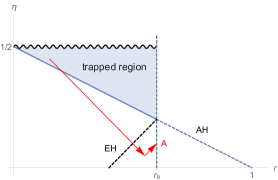
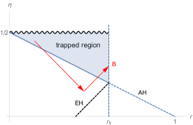
Figure 2: ($\eta,r$) diagram inside the stiff fluid $r\leq r_{b}$ for a space-like horizon ($\beta=-2$). Left: tunneling type-I path through the apparent (AH) and through the event horizon (EH). Right: tunneling type-I path only through the apparent horizon, therefore the radiation is not observable outside the event horizon.

The $(\eta,r)$ diagram is shown for the stiff fluid with $\beta=-2$ in Fig. 2 with

$$\eta=\frac{1}{2}[1-(1-t/t_{s})^{2/3}],$$ (49)

i.e. $\eta=1/2$ at $t_{s}=1/3$ and $\eta=0$ at $t=0$.

The apparent horizon formed during the collapse of the fluid sphere $r\leq r_{b}$ has its boundary at $a^{\beta}_{AH}=\frac{1}{r_{AH}}$ leading to

$$\eta_{AH}=-\frac{1}{\beta}(1-r)=\frac{1}{2}(1-r)~{}.$$ (50)

The event horizon inside the fluid boundary is determined by a radial light ray emitted at $r=0$ which just reaches the surface at $r=r_{b}$ at the same position as the apparent horizon

$$\eta_{EH}=r+\frac{1}{|\beta|}(1-r_{b})-r_{b}~{}=r+\frac{1}{2}-\frac{3r_{b}}{2}~{}.$$ (51)

Figure 3: ($t,R$) diagram with space-like horizon ($\beta=-2$) and tunneling type-I path (red) crossing the apparent (AH) and the event horizon (EH), finally reaching an external observer.

In Fig. 2 (left) we indicate a possible tunnelling path through the apparent horizon AH of the stiff fluid: the type-I path $\Delta r=-\Delta\eta>0$ starts in the trapped region, but crosses also the event horizon EH for $r\leq r_{b}$, outside the trapped region, before it reaches the particle-antiparticle vertex. Finally it crosses the boundary of the fluid at point A, which is outside the event horizon, ending at an outside observer; see also Fig. 3 (c.f. Fig. 4 in Vanzo:2011wq ). In Fig. 2 (right) the pair creation vertex is inside the EH, therefore the radiation is not observable for an outside observer.

In order to obtain the full spacetime the metric inside the collapsing fluid has to be matched with the outer region. We perform the matching by using the Schwarzschild metric.

Outside the collapsing fluid we choose the Schwarzschild metric

$$ds^{2}=-f(R)dT^{2}+\frac{dR^{2}}{f(R)}+R^{2}d\Omega_{2}^{2},~{}~{}f(R)=1-\frac{2M}{R},$$ (52)

which has to be matched with the interior FRW metric (3) at the boundary of a spherical junction hypersurface $r=r_{b}$. From the angular parts of the two metrics, we can identify at the boundary

$$R=r_{b}a(t)\equiv R_{b}(t),$$ (53)

where $t$ is the proper time of the collapsing fluid and $0\leq R_{b}\leq r_{b}$. From the Israel junction conditions, the Misner-Sharp mass (20) at the boundary is $2m(r_{b},t)=R_{b}(t)(1-f(R_{b}(t)))$, which then gives

$$2M(t)=\frac{R^{2\beta+1}_{b}(t)}{r_{b}^{2(\beta-1)}},$$ (54)

leading to a time-dependent mass $M(t)$. Note that $2M(t=0)=r^{3}_{b}$.

Following the treatment of gravitational collapse of uniform perfect fluids as described in Adler:2005vn , the Painlevé-Gullstrand coordinate system Poisson:2004 is well suited for the collapse under consideration. For the interior spacetime the radial coordinate R, Eq. (13), is introduced, leading to Eq. (25) with

$$\psi(R,t)=RH<0.$$ (55)

The exterior region with the metric (52) can be brought into the form of Painlevé-Gullstrand (24) by the transformation

$$T=t+g(R),$$ (56)

where

$$\frac{dg}{dR}=\frac{\psi}{1-\psi^{2}},~{}~{}\mbox{with}~{}~{}\psi^{2}=\frac{2M(t)}{R}.$$ (57)

In the following we discuss the case of the stiff fluid ($\beta=-2$). Introducing

$$R^{*}=\int\frac{dR}{f(R)}~{},$$ (58)

one derives after rescaling $R$ and $T$ by $r_{b}^{3/2}$:

$$R^{*}+T=R+t-\arctan R~{},$$ (59)

$$R^{*}-T=R-t-\frac{1}{2}\ln|\frac{1+R}{1-R}|~{}.$$ (60)

Finally, the Kruskal coordinates Hamilton read

$$r_{K}+t_{K}=\exp[(R^{*}+T)/2]~{},$$ (61)

and

$$\pm(r_{K}-t_{K})=\exp[(R^{*}-T)/2]~{},$$ (62)

depending on $R>1$ or $R<1$, resp. The corresponding diagram is shown in Fig. 4.

Figure 4: Space-like horizon ($\beta=-2$): Kruskal coordinates outside the stiff fluid. The radiation is indicated by the red arrows: only the one from A reaches the external observer at infinity.

IV.2 Time-like horizon

In case of a time-like horizon radiation is possible, as seen as follows: one takes a path with decreasing radial coordinate $\Delta r<0$, i.e. $\int_{\gamma}=-{\int\searrow}$ in Eq. (44) to obtain

$$\Im mI=-\frac{1}{\kappa_{H}}\Im m{\int\searrow}\frac{\omega}{r-r_{H}-i\epsilon}dr=-\frac{\pi\omega}{\kappa_{H}}~{},$$ (63)

such that the Hawking temperature becomes

$$T=-\frac{\kappa_{H}}{2\pi}~{},$$ (64)

which is positive for $\kappa_{H}(t)<0$, i.e. for time-like horizons: $-1<\beta<0$, in the FRW model under consideration.

For the typical case of the OS-model Oppenheimer:1939ue , with $\beta=-1/2$, a tunnelling path (type-II) with the vertex inside the trapped region and crossing the time-like horizon is possible, but the radiation ends at the center $r=0$. For the interior and exterior geometry of the collapsing sphere of dust see Fig. 7 in Hartle .

This case of Hawking radiation during the collapse of the fluid in the presence of a time-like dynamical horizon is trapped, see also the discussion in Ellis:2013oka ; Ellis:2014jja : it does not end up at infinity.

V Discussion

In summary to obtain the radiation temperature $T_{H}$ in the presence of a space-like or a time-like trapped horizon one may just take the absolute value in terms of the surface gravity on the horizon,

$$T_{H}=\frac{|\kappa_{H}|}{2\pi}~{}.$$ (65)

Concerning the regularization step one directly obtains this result - instead of using Eq. (44) - by considering as example the integral of an arbitrary function $f(r)\approx\kappa_{H}(r-r_{0})$ near the pole $r=r_{0}$, where $\kappa_{H}$ does not depend on $r$,

$$I=\Im m{\int\searrow}\frac{dr}{f(r)-i\epsilon}=$$ (66)

$$=\pi{\int\searrow}\delta[f(r)]dr=\frac{\pi}{|\partial_{r}f(r_{0})|}=\frac{\pi}{|\kappa_{H}|},$$ (67)

in terms of the absolute value of $\kappa_{H}$.

However, this consideration alone do not contain information if the Hawking radiation can reach an asymptotic observer. In order to decide this a more thorough investigation has to be made by checking if the Hawking radiation crosses both, the apparent and event horizons. In this note we reanalyzed the case of a collapsing fluid in a flat FRW background where we showed that only Hawking radiation from space-like trapping horizons can reach an external observer at infinity.

Acknowledgements We thank L. Vanzo for useful comments and A.B. Nielsen for discussions on earlier versions of this manuscript. S. Stricker was supported by the Austrian science Fund (FWF) under project P26328.

References

- (1) M. K. Parikh and F. Wilczek, Phys. Rev. Lett. 85 (2000) 5042 [hep-th/9907001].
- (2) M. Visser, “Essential and inessential features of Hawking radiation,” Int. J. Mod. Phys. D 12 (2003) 649 [hep-th/0106111].
- (3) for a review and references: L. Vanzo, G. Acquaviva and R. Di Criscienzo, “Tunnelling Methods and Hawking’s radiation: achievements and prospects,” Class. Quant. Grav. 28 (2011) 183001 [arXiv:1106.4153 [gr-qc]].
- (4) L. Vanzo, “Some results on dynamical black holes,” arXiv:0811.3532 [gr-qc].
- (5) A. B. Nielsen and M. Visser, “Production and decay of evolving horizons,” Class. Quant. Grav. 23 (2006) 4637 [gr-qc/0510083].
- (6) A. B. Nielsen, “Black holes and black hole thermodynamics without event horizons,” Gen. Rel. Grav. 41 (2009) 1539 [arXiv:0809.3850 [hep-th]].
- (7) D. W. Tian and I. Booth, “Apparent horizon and gravitational thermodynamics of the Universe: Solutions to the temperature and entropy confusions, and extensions to modified gravity,” arXiv:1411.6547 [gr-qc].
- (8) A. Ashtekar and B. Krishnan, “Isolated and dynamical horizons and their applications,” Living Rev. Rel. 7 (2004) 10 [gr-qc/0407042].
- (9) S. A. Hayward, R. Di Criscienzo, L. Vanzo, M. Nadalini and S. Zerbini, “Local Hawking temperature for dynamical black holes,” Class. Quant. Grav. 26 (2009) 062001 [arXiv:0806.0014 [gr-qc]].
- (10) R. Di Criscienzo, S. A. Hayward, M. Nadalini, L. Vanzo and S. Zerbini, “Hamilton-Jacobi tunneling method for dynamical horizons in different coordinate gauges,” Class. Quant. Grav. 27 (2010) 015006.
- (11) J. M. M. Senovilla and R. Torres, “Particle production from marginally trapped surfaces of general spacetimes,” arXiv:1409.6044 [gr-qc].
- (12) A. B. Nielsen, “Black Holes without Event Horizons,” J. Korean Phys. Soc. 54 (2009) 2576 [arXiv:0802.3422 [gr-qc]].
- (13) R. Baier, H. Nishimura and S. A. Stricker, “Scalar field collapse with negative cosmological constant,” Class. Quant. Grav. 32 (2015) 135021 [arXiv:1410.3495 [gr-qc]].
- (14) P. S. Joshi, “Global Aspects in Gravitation and Cosmology,” Oxford Univ. Press 2002.
- (15) P. S. Joshi, “Key problems in black hole physics today,” Bull. Astr. Soc. India 39 (2011) 1, arXiv:1104.3741 [gr-qc].
- (16) P. S. Joshi, “Gravitational Collapse and Spacetime Singularities,” Cambridge University Press, 2007.
- (17) P. S. Joshi and R. Goswami, “On trapped surface formation in gravitational collapse,” Class. Quant. Grav. 24 (2007) 2917.
- (18) “Black Holes - New Horizons,” ed. S. A. Hayward, World Scientific, 2013.
- (19) J. R. Oppenheimer and H. Snyder, “On continued gravitational contraction,” Phys. Rev. 56 (1939) 455.
- (20) R. J. Adler, J. D. Bjorken, P. Chen and J. S. Liu, “Simple analytic models of gravitational collapse,” Am. J. Phys. 73 (2005) 1148 [gr-qc/0502040].
- (21) S. A. Hayward, “General laws of black-hole dynamics,” Phys. Rev. D 49 (1994) 6467.
- (22) S. A. Hayward, “Gravitational energy in spherical symmetry,” Phys. Rev. D 53 (1996) 1938.
- (23) S. A. Hayward, “Black holes: New horizons,” [gr-qc/0008071].
- (24) I. Booth, “Black hole boundaries,” Can. J. Phys. 83 (2005) 1073 [gr-qc/0508107].
- (25) I. Booth, L. Brits, J. A. Gonzalez and C. Van Den Broeck, “Marginally trapped tubes and dynamical horizons,” Class. Quant. Grav. 23 (2006) 413 [gr-qc/0506119].
- (26) E. Poisson, “A Relativist’s Toolkit: The Mathematics of Black-Hole Mechanics,” Cambridge Univ. Press, 2004.
- (27) C. W. Misner and D. H. Sharp, “Relativistic equations for adiabatic, spherically symmetric gravitational collapse,” Phys. Rev. 136 (1964) B571.
- (28) S. A. Hayward, “Unified first law of black hole dynamics and relativistic thermodynamics,” Class. Quant. Grav. 15 (1998) 3147 [gr-qc/9710089].
- (29) M. Pielahn, G. Kunstatter and A. B. Nielsen, “Dynamical Surface Gravity in Spherically Symmetric Black Hole Formation,” Phys. Rev. D 84 (2011) 104008 [arXiv:1103.0750 [gr-qc]].
- (30) R. G. Cai, L. M. Cao and Y. P. Hu, “Hawking Radiation of Apparent Horizon in a FRW Universe,” Class. Quant. Grav. 26 (2009) 155018 [arXiv:0809.1554 [hep-th]].
- (31) St. Hawking and R. Penrose, “The nature of space and time,” Princeton Univ. Press, 1996.
- (32) S. W. Hawking, “Black hole explosions,” Nature 248 (1974) 30.
- (33) S. W. Hawking, “Particle Creation by Black Holes,” Commun. Math. Phys. 43 (1975) 199 [Erratum-ibid. 46 (1976) 206].
- (34) Andrew J. S. Hamilton, ” General Relativity, Black Holes, and Cosmology”, proto-book, 2014.
- (35) J. B. Hartle, ”Relativistic stars, gravitational collapse, and black holes”, in Relativity, Astrophysics and Cosmology, ed. W. Israel (Dordrecht, Reidel) p. 153, 1973.
- (36) G. F. R. Ellis, “Astrophysical black holes may radiate, but they do not evaporate,” arXiv:1310.4771 [gr-qc].
- (37) G. F. R. Ellis, R. Goswami, A. I. M. Hamid and S. D. Maharaj, “Astrophysical Black Hole horizons in a cosmological context: Nature and possible consequences on Hawking Radiation,” Phys. Rev. D 90 (2014) 8, 084013 [arXiv:1407.3577 [gr-qc]; and references therein.