Max-sum diversity via convex programming

Abstract

Diversity maximization is an important concept in information retrieval, computational geometry and operations research. Usually, it is a variant of the following problem: Given a ground set, constraints, and a function $f(\cdot)$ that measures diversity of a subset, the task is to select a feasible subset $S$ such that $f(S)$ is maximized. The sum-dispersion function $f(S)=\sum_{x,y\in S}d(x,y)$, which is the sum of the pairwise distances in $S$, is in this context a prominent diversification measure. The corresponding diversity maximization is the max-sum or sum-sum diversification. Many recent results deal with the design of constant-factor approximation algorithms of diversification problems involving sum-dispersion function under a matroid constraint.

In this paper, we present a PTAS for the max-sum diversification problem under a matroid constraint for distances $d(\cdot,\cdot)$ of negative type. Distances of negative type are, for example, metric distances stemming from the $\ell_{2}$ and $\ell_{1}$ norm, as well as the cosine or spherical, or Jaccard distance which are popular similarity metrics in web and image search.

Our algorithm is based on techniques developed in geometric algorithms like metric embeddings and convex optimization. We show that one can compute a fractional solution of the usually non-convex relaxation of the problem which yields an upper bound on the optimum integer solution. Starting from this fractional solution, we employ a deterministic rounding approach which only incurs a small loss in terms of objective, thus leading to a PTAS. This technique can be applied to other previously studied variants of the max-sum dispersion function, including combinations of diversity with linear-score maximization, improving the previous constant-factor approximation algorithms.

1 Introduction

Diversification is an important concept in many areas of computing such as information retrieval, computational geometry or optimization. When searching for news on a particular subject, for example, one is usually confronted with several relevant search results. A news-reader might be interested in news from various sources and viewpoints. Thus, on the one hand, the articles should be relevant to his search and, on the other hand, should be significantly diverse.

The so-called max-sum diversification or max-sum dispersion is a diversity-measure that has been subject of study in operations research [19, 28, 6, 4] for a while and it is currently receiving considerable attention in the information retrieval literature [16, 5, 8]. It is readily described. Given a ground set $X$ together with a distance function $d:X\times X\rightarrow\mathbb{R}_{\geqslant 0}$. The diversity, or dispersion, of a subset $S\subseteq X$ is the sum of the pairwise distances

$$f(S)=\sum_{i,j\in S}d(i,j).$$

Since documents are often represented as vectors in a high-dimensional space, their similarity is measured by norms in $\mathbb{R}^{n}$ and their induced distances, see, e.g., [24, 29]. Among the most frequent distances are the ones induced by the $\ell_{1}$ and $\ell_{2}$ norm, the cosine-distance or the Jaccard distance [26]. These norms are also used to measure similarity via much lower-dimensional bit-vectors stemming from sketching techniques [9]. So, usually, the ground set $X$ is a finite set of vectors in $\mathbb{R}^{d}$ and $d(\cdot,\cdot)$ is a metric on $\mathbb{R}^{d}$ which makes diversity maximization a geometric optimization problem.

Before we go on, we state the general version of the maximum sum diversification or maximum sum dispersion ($\mathrm{MSD}$) problem which generalizes many previously studied variants. It is in the focus of this paper, and is described by the following quadratic integer programming problem:

$$\begin{array}[]{ll}\text{maximize}&x^{T}Dx\\ \\ \text{subject to}&Ax\leqslant b\\ \\ &x_{i}\in\{0,1\}\,\text{ for }\,i\in[n],\end{array}$$ (1)

where the symmetric matrix $D\in\mathbb{R}^{n\times n}$ represents the distances between the points of a distance space and $Ax\leqslant b$ is a set of additional linear constraints where $A\in\mathbb{R}^{m\times n}$ and $b\in\mathbb{R}^{m}$. If $x\in\{0,1\}^{n}$ is the characteristic vector of the set $S\subseteq X$, then $x^{T}Dx=\sum_{i,j\in S}d(i,j)$. We recall the notion of a distance space, see, e.g., [12]. It is a pair $(X,d)$ where $X$ is a finite set and $d(\cdot,\cdot)$ is the distance function $d:X\times X\rightarrow\mathbb{R}_{\geqslant 0}$. The function $d$ satisfies $d({i,i})=0$ and $d({i,j})=d({j,i})$ for all $i,j\in X$. If in addition $d$ satisfies the triangle inequality $d({i,j})\leqslant d({i,k})+d({j,k})$ for all $i,j,k\in X$, then $d$ is a (semi) metric and $(X,d)$ a finite metric space.

We now mention some previous algorithmic work on diversity maximization with this objective function. For the case where $Ax\leqslant b$ represents one cardinality constraint, $\sum_{i=1}^{n}x_{i}\leqslant k,$ and $d(\cdot,\cdot)$ is a metric, the problem is also coined $\mathrm{MSD}_{k}$ [8]. Constant factor approximation algorithms for $\mathrm{MSD}_{k}$ have been developed in [28, 19]. Birnbaum and Goldman [6] presented an algorithm with approximation factor converging to $1/2$. This is tight under the assumption that the planted clique problem [3] is hard, see [8]. Baur and Fekete [4] have shown that this problem has a PTAS for $X\subset\mathbb{R}^{d}$ and $d(\cdot,\cdot)$ being the $\ell_{1}$-distance, provided that the dimension $d$ is fixed. Bhattacharya et al. [5] developed a $1/2$-approximation algorithm for $\mathrm{MSD}_{k}$ where the objective function is replaced by $x^{T}Dx+c^{T}x$ for some $c\in\mathbb{R}^{n}$. This has been useful in accommodating also scores of documents in the objective function.

Recently, Abbassi et al. [1] have shown that $\mathrm{MSD}$ has a $1/2$-approximation algorithm if $d(\cdot,\cdot)$ is a metric and $Ax\leqslant b$ models the independent sets of a matroid. This is particularly relevant in situations where documents are partitioned into subsets $D_{1},\dots,D_{\ell}$ and only $p_{i}$ results should be returned from partition $D_{i}$ for each $i$. The possible sets are then independent sets of a partition matroid. The case of one cardinality constraint only is subsumed by $\ell=1$. Thus, the tightness of their result also follows from the planted clique assumption as described in [8].

Contributions of this paper

The $\frac{1}{2}+\varepsilon$ hardness of $\mathrm{MSD}_{k}$ [8] is based on a metric that does not play a prominent role as a similarity measure. Are there better approximation algorithms, possibly polynomial time approximation schemes, for other relevant distance metrics?

We give a positive answer to this question for the case where $d(\cdot,\cdot)$ is a distance of negative type. We review the notion of negative-type distances in Section 2 and here only note that the previously mentioned distances, like the ones stemming from the $\ell_{2}$ and $\ell_{1}$-norm, as well as the cosine-distance and the Jaccard distance are, among many other relevant distance functions, of negative type. Our main result is the following.

Theorem 1.

There exists a polynomial time approximation scheme for $\mathrm{MSD}$ for the case that $d(\cdot,\cdot)$ is of negative type and $Ax\leqslant b$ is a matroid constraint. In particular, there is a polynomial time approximation scheme for $\mathrm{MSD}_{k}$ for negative type distances.

Theorem 1 is shown by following these two steps.

1. We show that one can compute a fractional solution $x^{*}\in\mathbb{R}^{n}$ that fulfills all the constraints $Ax\leqslant b$ and satisfies ${x^{*}}^{T}Dx^{*}\geqslant OPT$, where $OPT$ is the objective-function value of the optimal solution. More precisely, our algorithm does not optimize over the natural relaxation, but only over a family of slices of it, one for each possible $\ell_{1}$-norm of the solution vector. The key property we show and exploit is that the optimization problem on each slice is a convex optimization problem that can be attacked by standard techniques, despite the fact that the natural relaxation is not convex. This allows us to obtain an optimal solution to the relaxation via the ellipsoid method for a wide family of constraints $Ax\leqslant b$, even if only a separation oracle is given; in particular, this includes matroid polytopes [18].

2. For the case in which $Ax\leqslant b$ describes the convex hull of independent sets of a matroid, we furthermore describe a polynomial-time rounding algorithm that computes an integral feasible solution $\bar{x}$ which satisfies $\bar{x}^{T}D\bar{x}\geqslant\left(1-c\cdot\frac{\log k}{k}\right){x^{*}}^{T}D{x^{*}},$ for some universal constant $c$ and where $k$ is the rank of the matroid.

Thus, step a) is via a suitable convexification of a non-convex relaxation. Convexifications have proved useful in the design of approximation algorithms before, see for example [33].

We also want to mention that we obtain similar results for the case where the objective function is a combination of max-sum dispersion and linear scores, a scenario that has been considered in [5]. Finally, to complement our results, we prove $\mathrm{NP}$-hardness of $\mathrm{MSD}_{k}$ for negative type distances. We prove as well that, for the rounding algorithm mentioned in point b), the approximation factor of $1-O\left(\frac{\log k}{k}\right)$ almost matches the integrality gap of our relaxation, which we can show to be at least $1-\frac{1}{k}$.

2 Preliminaries

In this section, we review some preliminaries that are required for the understanding of this paper. A polynomial time approximation scheme (PTAS) for an optimization problem in which the objective function is maximized, is an algorithm that, given an instance and an $\varepsilon>0$, computes a solution that has an objective function value of at least $(1-\varepsilon)\cdot OPT$, where $OPT$ denotes the the objective function value of the optimal solution. Clearly, our rounding algorithm is a PTAS since we can compute the optimal solution in the case where $\varepsilon<c\cdot\frac{\log k}{k}$ by brute force.

Norms and embeddings

Our results rely heavily on the theory of embeddings. We review some notions that are relevant for us and refer to [12, 25] for a thorough account. For a vector $v=(v^{1},\cdots,v^{t})^{T}\in\mathbb{R}^{t}$, we define the $l_{p}$ norm in the usual way, $\|v\|_{\infty}:=\max_{1\leqslant i\leqslant t}|v^{i}|$, and $\|v\|_{p}:=(\sum_{i=1}^{t}|v^{i}|^{p})^{1/p}$ for $p\geqslant 1$, and we extend this last definition to $0<p<1$, even if they are not proper norms as they do not respect the triangle inequality. For $0<p\leqslant\infty$, the space $(X,d)$ is $l_{p}$-embeddable if there is a dimension $t$ and a function $v:X\rightarrow\mathbb{R}^{t}$ (the isometric embedding), such that for all $i,j\in X$ we have $d(i,j)=\|v_{j}-v_{i}\|_{p}$. Any finite metric space is $l_{\infty}$-embeddable with the Fréchet embedding [14] $v_{i}^{j}=d(i,j)$ for $i,j\in X$.

For the remainder of this paper, we assume that $X=\{1,\dots,n\}$ and $n\geqslant 2$. Let $b_{1},\dots,b_{n}$ be real coefficients. The inequality

$$\sum_{1\leqslant i,j\leqslant n}b_{i}b_{j}x_{ij}\leqslant 0$$ (2)

with variables $x_{ij}$ is a negative type inequality if $\sum_{i=1}^{n}b_{i}=0$. The distance space $(X,d)$ is of negative type if $d(\cdot,\cdot)$ satisfies all negative type inequalities, i.e., $\sum_{1\leqslant i,j\leqslant n}b_{i}b_{j}d(i,j)\leqslant 0$ holds for all $b_{1},\dots,b_{n}\in\mathbb{R}$ with $\sum_{i=1}^{n}b_{i}=0$. Schoenberg [30, 31] characterized the metric spaces that are $\ell_{2}$-embeddable as those, whose square distance is of negative type.

Theorem 2 ([30, 31]).

A finite distance space $(X,d)$ is of negative type if and only if $(X,\sqrt{d})$ is $\ell_{2}$-embeddable.

The following assertions, which help identifying distance spaces of negative type, can be found in [12].

1. If $(X,d)$ is a metric space, then $\left(X,d^{\log_{2}\left(\frac{n}{n-1}\right)}\right)$ is of negative type. [13]

2. For any $0<\alpha\leqslant p\leqslant 2,$ if $(X,d)$ is $l_{p}$-embeddable, then $(X,d^{\alpha})$ is of negative type. [31]

3. If $(X,d)$ is of negative type, then $(X,f(d))$ is also of negative type for any of the following functions: $f(x)=\frac{x}{1+x}$, $f(x)=\ln(1+x)$, $f(x)=1-e^{-\lambda x}$ for $\lambda>0$, and $f(x)=x^{\alpha}$ for $0\leqslant\alpha\leqslant 1$. [30]

We now list some distance functions that are of negative type and which are often used in information retrieval and web search. The $\ell_{1}$-metric is of negative type. This follows from the assertion ii) above with $\alpha=p=1$. In fact, any $\ell_{p}$-metric with $1\leqslant p\leqslant 2$ is of negative type. The $\ell_{1}$-metric is a prominent similarity measure in information retrieval [24] in particular when using sketching techniques [22] where data points are represented by small-dimensional bit-vectors whose Hamming-distance approximates the distance of the corresponding points. Also the cosine distance, which measures the distance of two points on the sphere $S^{(t-1)}$ by the angle that they enclose, is of negative type. This follows from a result of Blumenthal [7], see also [12]. For subsets $A,B$ of a finite ground set $U$, the Jaccard distance $d(A,B)=1-\frac{|A\cap B|}{|A\cup B|}$ is of negative type [17]. Similarly, many other distances of sets are of negative type, such as Simple Matching $\frac{|A\bigtriangleup B|}{|U|}$, Russell and Rao $1-\frac{|A\cap B|}{|U|}$, and Dice $\frac{|A\bigtriangleup B|}{|A|+|B|}$ distances (see [26, Table 5.1] for a more complete list). Assertion iii) above presents some examples of transformations of distance spaces that preserve this property, and thus permit to construct new spaces of negative type from existing ones.

It is important to remark that distance spaces of negative type are in general not metric, or vice-versa. Hence results for these two families of distance spaces are not directly comparable. For instance, the Dice distance mentioned before is not metric.

Matroids and the matroid polytope

We mention some basic definitions and results on matroid theory, see, e.g., [32, Volume B] for a thorough account. A matroid $\mathcal{M}$ over a finite ground set $X$ is a tuple $\mathcal{M}=(X,\mathcal{I})$, where $\mathcal{I}\subseteq 2^{X}$ is a family of independent sets with the following properties.

• $\emptyset\in\mathcal{I}$.

• If $A\subseteq B$ and $B\in\mathcal{I}$, then $A\in\mathcal{I}$.

• If $A,B\in\mathcal{I}$ and $|A|>|B|$, then there exists an element $e\in A\setminus B$ such that $B\cup\{e\}\in\mathcal{I}$.

In particular, the family of all subsets of $X$ of cardinality at most $k$, i.e., $\mathcal{I}=\{S\subseteq X\colon\mid S\mid\leqslant k\}$, forms a matroid known as uniform matroid of rank $k$, often denoted by $U_{n}^{k}$. Thus, $\mathrm{MSD}_{k}$ can be understood as picking an independent set $S\in\mathcal{I}$ from the uniform matroid that maximizes the sum of the pairwise distances.

The rank $r(A)$ of $A\subseteq X$ is the maximum cardinality of an independent set contained in $A$. Any inclusion-wise maximal independent set $B$ is called a basis, and a direct consequence of the definition of matroids is that all bases have the same cardinality $r(X)$, called the rank of the matroid.

The matroid polytope $P(\mathcal{M})$ is the convex hull of the characteristic vectors of the independents sets of the matroid $\mathcal{M}$. It can be described by the following inequalities $P(\mathcal{M})=\{x\in\mathbb{R}^{n}_{\geqslant 0}\colon\sum_{i\in A}x_{i}\leqslant r(A)\ \forall A\subseteq X\}$. The base polytope of a matroid $\mathcal{M}$ of rank $k$ is the convex hull of all characteristic vectors of bases of $\mathcal{M}$, and is given by $P(\mathcal{M})\cap\{x\in\mathbb{R}^{n}\colon\sum_{i=1}^{n}x_{i}=k\}$.

Convex quadratic programming

A quadratic program is an optimization problem of the form

$$\min\{x^{T}Qx+c^{T}x\colon x\in\mathbb{R}^{n},\,Ax\leqslant b\},$$

where $Q\in\mathbb{R}^{n\times n}$, $c\in\mathbb{R}^{n}$, $A\in\mathbb{R}^{m\times n}$ and $b\in\mathbb{R}^{m}$. If $Q$ is positive semidefinite, then it is a convex quadratic program. Convex quadratic programs can be solved in polynomial time with the ellipsoid method [20], see, e.g., [21]. This also holds if $Ax\leqslant b$ is not explicitly given but the separation problem for $Ax\leqslant b$ can be solved in polynomial time [18]. In this case the running time is polynomial in the input size of $D$ and the largest binary encoding length of the coefficients in $A$ and numbers in $b$. The separation problem for the matroid polytope $P(\mathcal{M})$ can be solved in polynomial time, provided that one can efficiently decide whether a set $S\subseteq X$ is an independent set, see [18]. Moreover, the largest encoding length of the numbers in the above-mentioned description of the matroid polytope is $O(\log n)$. Thus a convex quadratic program over the matroid polytope can be solved in polynomial time.

3 A relaxation that can be solved by convex programming

We now describe how to efficiently compute a fractional point $x^{*}$ for the relaxation of (1) with an objective value ${x^{*}}^{T}Dx^{*}\geqslant OPT$. The function $f:\mathbb{R}^{n}\rightarrow\mathbb{R}$, $f(x)=x^{T}Dx$ is in general non-concave, even if the distances $d(i,j)$ are $\ell_{2}$-embeddable or of negative type. However, we have the following useful observation.

Lemma 3.

Let $(X,d)$ be a finite distance space of negative type, then

$$f(x)=x^{T}Dx$$

is a concave function over the domain $\{x\in\mathbb{R}^{n}\colon\sum_{i=1}^{n}x_{i}=\alpha\}$ for each fixed $\alpha\in\mathbb{R}$.

Proof.

By Theorem 2, the distance $\sqrt{d}$ is $\ell_{2}$-embeddable; let $v_{1},\dots v_{n}\in\mathbb{R}^{t}$ be a corresponding embedding, i.e.,

$$d(i,j) = \lVert v_{i}-v_{j}\rVert_{2}^{2}$$

$$= (v_{i}-v_{j})^{T}(v_{i}-v_{j})$$

$$= \lVert v_{i}\rVert_{2}^{2}-2v_{i}^{T}v_{j}+\lVert v_{j}\rVert_{2}^{2}.$$

For $x\in\mathbb{R}^{n}$ with $\sum_{i=1}^{n}x_{i}=\alpha$, $x^{T}Dx$ can be written as

$$x^{T}Dx = \sum_{1\leqslant i,j\leqslant n}x_{i}x_{j}\left(\lVert v_{i}\rVert_{2}^{2}-2v_{i}^{T}v_{j}+\lVert v_{j}\rVert_{2}^{2}\right)$$

$$= \sum_{j=1}^{n}x_{j}\sum_{i=1}^{n}(x_{i}\lVert v_{i}\rVert_{2}^{2})-2\sum_{1\leqslant i,j\leqslant n}x_{i}(v_{i}^{T}v_{j})x_{j}+\sum_{i=1}^{n}x_{i}\sum_{j=1}^{n}(x_{j}\lVert v_{j}\rVert_{2}^{2})$$

$$= 2\alpha c^{T}x-2\cdot x^{T}Qx,$$

where $Q\in\mathbb{R}^{n\times n}$ is the positive semidefinite matrix with $Q_{ij}=v_{i}^{T}v_{j}$, hence $x^{T}Qx$ is convex, and $c\in\mathbb{R}^{n}$ is the vector $c^{T}=(\lVert v_{1}\rVert_{2}^{2},\dots,\lVert v_{n}\rVert_{2}^{2})$. Thus $x^{T}Dx$ is concave on the domain $\{x\in\mathbb{R}^{n}\colon\sum_{i=1}^{n}x_{i}=\alpha\}$. ∎

Remark 1.

Notice that the matrix $Q$ and the vector $c$ can easily be derived from the distances. For this observe that if $v_{1},\dots,v_{n}\in\mathbb{R}^{t}$ is an embedding of $\sqrt{d}$, then $v_{1}-u,v_{2}-u,\dots,v_{n}-u$ is another such embedding, for each $u\in\mathbb{R}^{t}$. Hence, we can assume $v_{1}=\mathbf{0}$, which implies $c_{i}=\lVert v_{i}\rVert_{2}^{2}=d(1,i)$ and thus $Q_{ij}=\frac{1}{2}\left(d(1,i)+d(1,j)-d(i,j)\right)$. Hence, the embedding does not need to be known to describe $Q$ and $c$.

Using Lemma 3, we can efficiently determine a relaxed solution for $\mathrm{MSD}$ on distance spaces of negative type for a wide class of constraints, by solving a family of convex problems, one for each possible $\ell_{1}$ norm of the solution vector. There is a rich set of algorithms for convex optimization problems as we encounter here. In the following theorem, for simplicity, we focus on consequences stemming from the ellipsoid algorithm. The ellipsoid algorithm has the advantage that it only needs a separation oracle, and often allows us to obtain an optimal solution without any error. As a technical requirement, we need that the coefficients of the underlying linear constraints have small encoding lengths, which holds for most natural constraints.

Theorem 4.

Consider the max-sum dispersion problem with general linear constraints, for which the separation problem can be solved in polynomial time

$$\begin{array}[]{ll}\text{maximize}&x^{T}Dx\\ \\ \text{subject to}&Ax\leqslant b\\ \\ &x_{i}\in\{0,1\}\,\text{ for }\,i\in X.\end{array}$$ (3)

If $d(\cdot,\cdot)$ is of negative type, then one can compute a fractional point $x^{*}\in[0,1]^{n}$ satisfying $Ax\leqslant b$ with ${x^{*}}^{T}Dx^{*}\geqslant OPT$ in time polynomial in the input and the maximal binary encoding length of any coefficient or right-hand side of $Ax\leqslant b$.

Before proving the theorem, we briefly discuss the above-mentioned dependence of the running time on the encoding length. Notice that if $Ax\leqslant b$ is given explicitly, then the claimed point $x^{*}$ is always obtained in polynomial time because the encoding length of $Ax\leqslant b$ is part of the input. Similarly, Theorem 4 implies that we can obtain $x^{*}$ efficiently for matroid polytopes, since the inequality-description mentioned in Section 2 has only $\{0,1\}$-coefficients and right-hand sides within $\{1,\dots,n\}$. We highlight that our techniques can often be used even if the encoding length condition is not fulfilled by accepting a small additive error.

Proof.

Consider the constraints $\sum_{i=1}^{n}x_{i}=\alpha$ for $\alpha\in\{1,\dots,n\}$. Using the notation of Lemma 3, we can re-write the objective function as $2\alpha c^{T}x-2\cdot x^{T}Qx$ if the constraint $\sum_{i=1}^{n}x_{i}=\alpha$ is added to the constraints $Ax\leqslant b$. Using the ellipsoid method, we solve each of the following $n$ convex quadratic programming problems that are parameterized by $\alpha\in\{1,\dots,n\}$

$$\begin{array}[]{ll}\text{minimize}&2\cdot x^{T}Qx-2\alpha c^{T}x\\ \\ \text{subject to}&Ax\leqslant b\\ \\ &\sum_{i=1}^{n}x_{i}=\alpha\\ \\ &0\leqslant x_{i}\leqslant 1,\text{ for }\,i\in X,\end{array}$$ (4)

with optimum solutions $x^{*,1},\dots,x^{*,n}$ respectively; see [21, 18] for details on why an optimal solution can be obtained (without any additive error which is typical for many convex optimization techniques). Since each feasible $\bar{x}\in\{0,1\}^{n}$ satisfies one of these constraints, $x^{*}$ being one of these solutions with largest objective function value is a point satisfying the claim. Clearly, $x^{*}$ can be computed in polynomial time. ∎

Remark 2.

We notice that for very simple constraints, like a cardinality constraint where at most $k$ elements can be picked, a randomized rounding approach [27] can now be employed. More precisely, when working with a cardinality constraint one can simply scale down the fractional solution $x^{*}$ satisfying $\sum_{i=1}^{n}x_{i}^{*}=k$ by a $(1-\varepsilon)$-factor to obtain $y=(1-\varepsilon)x^{*}$, and then round each component of $y$ independently. Independent rounding preserves the objective in expectation, and the number of picked elements is $(1-\varepsilon)k$ in expectation and sharply concentrates around this value due to Chernoff-type concentration bounds. However, this simple rounding approach fails for more interesting constraint families like matroid constraints.

4 Negative type MSD under matroid constraint

Consider the MSD problem for the case that the distance space is of negative type and $Ax\leqslant b$ is a matroid constraint. The main result of this section is the following theorem which immediately implies Theorem 1.

Theorem 5.

There exists a deterministic algorithm for the $\mathrm{MSD}$ problem in distance spaces of negative type with a matroid constraint, which outputs in polynomial time a basis $B$ with $\left({\chi^{B}}\right)^{T}D\chi^{B}\geqslant\left(1-c\frac{\log k}{k}\right)\mathrm{OPT}$, where $k$ is the rank of the matroid and $c$ is an absolute constant.

We solve the relaxation to obtain an optimal fractional point over the matroid polytope, as in Theorem 4, and perform a deterministic rounding algorithm. The suggested rounding procedure has similarities with pipage rounding for matroid polytopes (see [11], which is based on work in [2]) and swap rounding [10], in the sense that it iteratively changes at most two components of the fractional point until an integral point is obtained. However contrary to these previous procedures we need to judiciously choose the two coordinates. Also our analysis differs substantially from the above-mentioned prior rounding procedures on matroids, since we deal with a quadratic objective function were we must accept a certain loss in the objective value due to rounding, because there is a strictly positive integrality gap. (Pipage rounding and swap rounding are typically applied in settings where the objective function is preserved in expectation.) Makarychev, Schudy, and Sviridenko [23] build up on the swap rounding procedure and show how to obtain concentration bounds for polynomial objective functions. Their concentration results apply to general polynomial objective functions with coefficients in $[0,1]$; however, they are not strong enough for our purposes.

Our deterministic rounding algorithm exploits the fact that we are dealing with negative type distance spaces, and shows that only a very small loss in the objective value is necessary to obtain an integral solution. In order to bound this loss we use a very general inequality, stemming from the definition of distance spaces of negative type, that compares the (fractional) dispersion of two sets to that of its union. Given a vector $x\in\mathbb{R}^{n}$ and a set $S\subseteq\{1,\cdots,n\}$, we define the restricted vector $x^{S}$ as $x^{S}_{i}=x_{i}$ if $i\in S$, and 0 otherwise.

Lemma 6.

Let $D\in\mathbb{R}^{n\times n}$ be the matrix representing a negative type distance space. Given a vector $x\in\mathbb{R}^{n}_{\geqslant 0}$ of coefficients, and two disjoint sets $A,B\subseteq[n]$ such that $\|x^{A}\|_{1}>0$ and $\|x^{B}\|_{1}>0$, we have

$$\frac{\left({x^{A\cup B}}\right)^{T}Dx^{A\cup B}}{\|x^{A\cup B}\|_{1}}\geqslant\frac{\left({x^{A}}\right)^{T}Dx^{A}}{\|x^{A}\|_{1}}+\frac{\left({x^{B}}\right)^{T}Dx^{B}}{\|x^{B}\|_{1}}.$$

Proof.

Define the vector $b\in\mathbb{R}^{n}$ as $b=\frac{x^{A}}{\|x^{A}\|_{1}}-\frac{x^{B}}{\|x^{B}\|_{1}}$. Since $\sum_{i=1}^{n}b_{i}=0$, the inequality $b^{T}Db\leqslant 0$ is of negative type. Expanding it yields

$$0\geqslant\left(\frac{x^{A}}{\|x^{A}\|_{1}}-\frac{x^{B}}{\|x^{B}\|_{1}}\right)^{T}D\left(\frac{x^{A}}{\|x^{A}\|_{1}}-\frac{x^{B}}{\|x^{B}\|_{1}}\right)=\frac{\left({x^{A}}\right)^{T}Dx^{A}}{\|x^{A}\|_{1}^{2}}+\frac{\left({x^{B}}\right)^{T}Dx^{B}}{\|x^{B}\|_{1}^{2}}-2\frac{\left({x^{A}}\right)^{T}Dx^{B}}{\|x^{A}\|_{1}\|x^{B}\|_{1}}.$$

Hence $2\left({x^{A}}\right)^{T}Dx^{B}\geqslant\frac{\|x^{B}\|_{1}}{\|x^{A}\|_{1}}\left({x^{A}}\right)^{T}Dx^{A}+\frac{\|x^{A}\|_{1}}{\|x^{B}\|_{1}}\left({x^{B}}\right)^{T}Dx^{B}.$ Finally,

$${\left(x^{A\cup B}\right)}^{T}Dx^{A\cup B}= \left(x^{A}+x^{B}\right)^{T}D(x^{A}+x^{B})=\left({x^{A}}\right)^{T}Dx^{A}+\left({x^{B}}\right)^{T}Dx^{B}+2\left({x^{A}}\right)^{T}Dx^{B}$$

$$\geqslant \left(\|x^{A}\|_{1}+\|x^{B}\|_{1}\right)\left(\frac{\left({x^{A}}\right)^{T}Dx^{A}}{\|x^{A}\|_{1}}+\frac{\left({x^{B}}\right)^{T}Dx^{B}}{\|x^{B}\|_{1}}\right)$$

$$= \|x^{A\cup B}\|_{1}\left(\frac{\left({x^{A}}\right)^{T}Dx^{A}}{\|x^{A}\|_{1}}+\frac{\left({x^{B}}\right)^{T}Dx^{B}}{\|x^{B}\|_{1}}\right).$$

∎

Consider an MSD instance consisting of a distance space of negative type represented by a matrix $D\in\mathbb{R}^{n\times n}$, and a matroid $\mathcal{M}$ over the ground set $X=\{1,\ldots,n\}$ of rank $k$. We assume that one can efficiently decide whether a set $S\subseteq X$ is independent. So we apply Theorem 4 to find a fractional vector $x^{*}$ over the matroid polytope $P(\mathcal{M})=\left\{x\in\mathbb{R}^{n}_{\geqslant 0}\colon\sum_{i\in A}x_{i}\leqslant r(A)\ \forall A\subseteq X\right\}$, with $\left({x^{*}}\right)^{T}Dx^{*}\geqslant\mathrm{OPT}$. Due to the monotonicity of the diversity function $x^{T}Dx$, we can assume that $\|x^{*}\|_{1}=k$, i.e., $x^{*}$ is on the base polytope of the matroid $\mathcal{M}$. We describe now a deterministic rounding algorithm that takes $x^{*}$ as input, and outputs in polynomial time a basis $B$ of $\mathcal{M}$ with $\left({\chi^{B}}\right)^{T}D\chi^{B}\geqslant\left(1-O\left(\frac{\log k}{k}\right)\right)\left({x^{*}}\right)^{T}Dx^{*}\geqslant\left(1-O\left(\frac{\log k}{k}\right)\right)\mathrm{OPT}$.

In the remainder of the section, for any vector $x\in P(\mathcal{M})$ we ignore the elements $i$ with $x_{i}=0$ and assume without loss of generality that $x$ has no zero components. We call an element $i\in X$ integral or fractional (with respect to $x$), respectively, if $x_{i}=1$ or $x_{i}<1$, and we call a set $S\subseteq X$ tight or loose, respectively, if $\|x^{S}\|_{1}=r(S)$ or $\|x^{S}\|_{1}<r(S)$. We will need the following result about faces of the matroid polytope, which is a well-known consequence of combinatorial uncrossing (see [15], or [32, Section 44.6c in Volume B]).

Lemma 7.

Let $x\in P(\mathcal{M})$ with $x_{i}\neq 0$ for $i\in\{1,\dots,n\}$, and let $\emptyset=S_{0}\subsetneq S_{1}\subsetneq\cdots\subsetneq S_{p}=X$ be a (inclusion-wise) maximal chain of tight sets with respect to $x$, i.e., $\sum_{i\in S_{l}}x_{i}=r(S_{l})$ for $l\in\{1,\dots,p\}$. Then the polytope $P(\mathcal{M})\cap\{y\in\mathbb{R}^{n}_{\geqslant 0}\colon\sum_{i\in S_{l}}x_{i}=r(S_{l})\text{ for }l\in\{1,\dots,p\}\}$ defines the minimal face of $P(\mathcal{M})$ that contains $x$. (In other words, all other $x$-tight sets are implied by the ones in the chain.)

Also, given a point $x\in P(\mathcal{M})$, one can efficiently find a maximal chain of tight sets as described in Lemma 7. Our algorithm starts with such a chain $\emptyset=S_{0}\subsetneq S_{1}\subsetneq\cdots\subsetneq S_{p}=X$ for the vector $x^{*}$. For $1\leqslant l\leqslant p$ define the set $R_{l}=S_{l}\setminus S_{l-1}$; we call these sets rings. The rings form a partition of $X$, their weights $\|\left({x^{*}}\right)^{R_{l}}\|_{1}=r(S_{l})-r(S_{l-1})$ are strictly positive integers whose sum is $k$, and each ring $R_{l}$ either consists of a single integral element, or of at least 2 elements, all fractional. This is because whenever $i\in R_{l}$ is integral, the set $S_{l-1}\cup\{i\}$ is tight, so it can be added to the chain. We call the rings integral or fractional, accordingly. We start with $x=x^{*}$, we iteratively change two coordinates of $x^{*}$ without leaving the minimal face of the matroid polytope on which $x^{*}$ lies; one coordinate will be increased and the other one decreased by the same amount.

The rounding procedure

The rounding of $x^{*}$ proceeds in iterations, and stops when all elements are integral. Among all pairs of fractional elements within the same ring, select the pair $i,j$ that minimizes the term $x_{i}x_{j}d(i,j)$. We perturb vector $x$ by adding to $x_{i}$ and subtracting from $x_{j}$ a certain quantity $\varepsilon$. The dispersion $x^{T}Dx$ is linear in $\varepsilon$ except for the term $2x_{i}x_{j}d(i,j)$, hence we can select the sign of $\varepsilon$ so that the value of $x^{T}Dx-2x_{i}x_{j}d(i,j)$ does not decrease. We assume without loss of generality that this choice is $\varepsilon>0$, so $x_{i}$ is increasing and $x_{j}$ decreasing. We increment $\varepsilon$ until a new tight constraint appears. If the constraint corresponds to $x_{j}$ becoming zero, we erase that element and end the iteration step. Otherwise, a previously loose set $S\subseteq X$ becomes tight, and $S$ must contain $i$ but not $j$, else its weight $\|x^{S}\|_{1}$ would not increase during this process. If the ring containing $i$ and $j$ is $R_{l}=S_{l}\setminus S_{l-1}$, then the set $S^{\prime}=(S\cup S_{l-1})\cap S_{l}$ is also tight, and it also contains $i$ but not $j$, hence $S_{l_{1}}\subsetneq S^{\prime}\subsetneq S_{l}$ (see Figure 1). We add $S^{\prime}$ to the chain, update the list of rings, and end the iteration step.

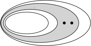
(a) The fractional ring containing the pair $i,j$ with minimal value $x^{m}_{i}x^{m}_{i}d(i,j)$.

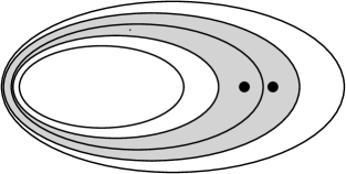
(b) Elements $i$ and $j$ are separated by a new tight set that fits in the chain structure.

Figure 1: The refinement of a fractional ring in an iteration of the rounding procedure.

We now argue that the above-described rounding procedure runs in polynomial time and computes the characteristic vector $\chi^{B}$ of a basis $B$ of the matroid $\mathcal{M}$ with

$$\left({\chi^{B}}\right)^{T}D\chi^{B}\geqslant\left(1-c\frac{\log k}{k}\right){x^{*}}^{T}Dx^{*}$$ (5)

where $k$ is the rank of the matroid and $c$ is an absolute constant.

At any stage of the algorithm, if $q$ is the number of fractional rings and $f$ is the number of fractional elements, the number of iterations remaining is at most $f-q$. This is because the value $f-q$ can never be negative, and it decreases in each iteration. Either $f$ decreases, or $q$ increases, or $q$ decreases by 1 but $f$ decreases by at least 2 (any disappearing fractional ring has at least 2 fractional elements that become integral).

Suppose there are $M$ iterations. We enumerate them in reverse order, and add a superscript $m$ to all variables to signify their value when there are $m$ iterations remaining. Hence $x^{0}=\chi^{B}$ is the integral output vector, $x^{1}$ is the vector at the beginning of the last iteration, and so on until $x^{M}=x^{*}$. Clearly, all vectors $x^{m}$ are in $P(\mathcal{M})$, and their weights $\|x^{m}\|_{1}=k$ remain unchanged, so each $x^{m}$ is on the base polytope, and $x^{0}$ will thus be a characteristic vector of a basis in $\mathcal{M}$. From the previous claim we know that $m\leqslant f^{m}-q^{m}$, and in particular $M\leqslant n$, so the algorithm runs in polynomial time. For $1\leqslant m\leqslant M$, define $\mathrm{loss}^{m}=\left({x^{m}}\right)^{T}Dx^{m}-\left({x^{m-1}}\right)^{T}Dx^{m-1}$, so the total additive loss incurred in the rounding algorithm is $\sum_{m=1}^{M}\mathrm{loss}^{m}$. We postpone for a moment the proof of the following inequality.

Lemma 8.

The loss in iteration $m$ is bounded by

$$\mathrm{loss}^{m}\leqslant\min\left\{\frac{2}{m\cdot k},\frac{2}{m^{2}}\right\}{x^{*}}^{T}Dx^{*}.$$

The total additive loss incurred by the algorithm is

$$\left({x^{*}}\right)^{T}Dx^{*}-\left({x^{0}}\right)^{T}Dx^{0} =\sum_{m=1}^{M}\mathrm{loss}^{m}\leqslant\left({x^{*}}\right)^{T}Dx^{*}\left(\sum_{m=1}^{k}\frac{2}{m\cdot k}+\sum_{m>k}\frac{2}{m^{2}}\ \right)$$

$$\leqslant\left({x^{*}}\right)^{T}Dx^{*}\cdot 2\left(\frac{1+\ln k}{k}+\frac{1}{k}\right)=\left({x^{*}}\right)^{T}Dx^{*}\cdot\left(\frac{4+2\ln k}{k}\right)\enspace,$$

where the second inequality follows from $\sum_{m=1}^{k}\frac{1}{m}\leqslant 1+\ln k$ and $\sum_{m>k}\frac{1}{m^{2}}\leqslant\frac{1}{k}$. In summary, the algorithm finds a basis with dispersion

$$\left({x^{0}}\right)^{T}D{x^{0}}\geqslant\left({x^{*}}\right)^{T}Dx^{*}\left(1-\frac{4+2\ln k}{k}\right)\geqslant\mathrm{OPT}\left(1-O\left(\frac{\log k}{k}\right)\right)$$

which is our main result.

Proof of Lemma 8.

If the pair $i,j$ of fractional elements is chosen during the $m$-th iteration, then $\mathrm{loss}^{m}\leqslant 2x^{m}_{i}x^{m}_{j}d(i,j)$. We bound this term from above, using the inequality in Lemma 6 multiple times over the vector $x^{m}$ and its partition into rings. We skip the superscript $m$ to simplify notation and obtain

$$\frac{x^{T}Dx}{k}\geqslant\sum_{\text{ring }R}\frac{\left({x^{R}}\right)^{T}Dx^{R}}{\|x^{R}\|_{1}}\geqslant\sum_{\text{fractional }R}\frac{\left({x^{R}}\right)^{T}Dx^{R}}{\|x^{R}\|_{1}}\geqslant\sum_{\text{fractional }R}\frac{\binom{|R|}{2}\mathrm{loss}}{\|x^{R}\|_{1}}\enspace,$$

where the last inequality comes from $\mathrm{loss}^{m}\leqslant 2x^{m}_{i}x^{m}_{j}d(i,j)$, and the choice of elements $i$ and $j$ that minimizes this quantity over all pairs of elements within any fractional ring. We complete the above inequality in two ways. First, for every fractional ring $R$, $|R|\geqslant\|x^{R}\|_{1}$, so $\frac{\binom{|R|}{2}}{\|x^{R}\|_{1}}\geqslant\frac{|R|-1}{2}$ and thus

$$\frac{x^{T}Dx}{k}\geqslant\frac{\mathrm{loss}}{2}\sum_{\text{frac. }R}(|R|-1)=\frac{\mathrm{loss}}{2}(f-q)\geqslant\frac{m}{2}\mathrm{loss}\enspace,$$

which implies

$$\mathrm{loss}^{m}\leqslant\frac{2}{m\cdot k}\left({x^{m}}\right)^{T}Dx^{m}\leqslant\frac{2}{m\cdot k}\left({x^{*}}\right)^{T}Dx^{*}\enspace.$$

Next, $\binom{|R|}{2}\geqslant(|R|-1)^{2}/2$, and using a Cauchy-Schwarz inequality (for the third inequality below), we get:

$$x^{T}Dx^{T}\geqslant \frac{k\cdot\mathrm{loss}}{2}\sum_{\text{frac. }R}\frac{(|R|-1)^{2}}{\|x^{R}\|_{1}}\geqslant\frac{\mathrm{loss}}{2}\left(\sum_{\text{frac. }R}\|x^{R}\|_{1}\right)\left(\sum_{\text{frac. }R}\frac{(|R|-1)^{2}}{\|x^{R}\|_{1}}\right)$$

$$\geqslant \frac{\mathrm{loss}}{2}\left(\sum_{\text{frac.}R}(|R|-1)\right)^{2}=\frac{\mathrm{loss}}{2}(f-q)^{2}\geqslant\frac{m^{2}}{2}\mathrm{loss}\enspace,$$

and hence,

$$\mathrm{loss}^{m}\leqslant\frac{2}{m^{2}}\left({x^{m}}\right)^{T}Dx^{m}\leqslant\frac{2}{m^{2}}\left({x^{*}}\right)^{T}Dx^{*}\enspace.$$

∎

Remark 3.

The integrality gap of the convex program $\max\{x^{T}Dx\ |\ x\in P(\mathcal{M})\}$ above is at least $1-\frac{1}{k}$, which matches the approximation factor of our rounding algorithm up to a logarithmic term. Consider the matrix $D$ with $D_{i,j}=1$ for all $i\neq j$, which defines a distance space of negative type, and a cardinality constraint corresponding to the polytope $\left\{x\in[0,1]^{n}\ |\ \sum_{i}x_{i}=k\right\}$. An optimal solution is any $k$-set $B\subseteq X$, with value $\mathrm{OPT}=(\chi^{B})^{T}D\chi^{B}=k(k-1)$; but the fractional vector $x^{*}=(k/n,\cdots,k/n)$ is feasible and has value $(x^{*})^{T}Dx^{*}=\frac{k^{2}}{n^{2}}n(n-1)$. Hence, $\frac{\mathrm{OPT}}{(x^{*})^{T}Dx^{*}}=\frac{k-1}{k}\frac{n}{n-1}\rightarrow 1-\frac{1}{k}$, as $n\rightarrow\infty$.

Remark 4.

The previous approximation extends to the more general case of a combination of dispersion and linear scores, as follows. Consider the problem of maximizing the objective function $g(x)=x^{T}Dx+w^{T}x$, with a matroid constraint of rank $k$, and where $D$ represents a distance space of negative type. The vector $w$ here corresponds to non-negative scores on the elements of the ground set, and the objective is to find a feasible set with both high dispersion and high scores. The extra linear term does not change the concavity of $x^{T}Dx$, so Lemma 3 and Theorem 5 are valid for this problem and provide a fractional vector $x^{*}\in P(\mathcal{M})$ with $g(x^{*})\geqslant\mathrm{OPT}$. Moreover, $g(x)$ is still monotone, so we can assume that $\|x^{*}\|_{1}=k$. In each iteration of this section’s rounding algorithm, $g(x)-2x_{i}x_{j}d(i,j)$ is linear in $\varepsilon$, so we can bound the loss of value of $g(x)$ during this iteration by $2x_{i}x_{j}d(i,j)$, as before. Hence, the above analysis still holds and shows that the total loss is very small, even when comparing it only to the contribution of the quadratic term $(x^{*})^{T}Dx^{*}$ to the objective, thus ignoring the additional nonnegative term $w^{T}x^{*}$. Thus, we get the same approximation guarantee for this setting.

To conclude, we prove that $\mathrm{MSD}$ remains $\mathrm{NP}$-hard on distance spaces of negative type, even for a cardinality constraint. For this, we give a reduction from Densest $k$-Subgraph (D$k$S), which is $\mathrm{NP}$-hard. An instance of D$k$S consists of a graph $G=(V,E)$ and a number $k\leqslant n=|V|$, and the object is to find a $k$-set $W\subseteq V$ whose induced subgraph $G[W]$ contains the largest number of edges. Now, the distance function $d^{\prime}:V^{2}\to\mathbb{R}_{\geqslant 0}$ defined by $d^{\prime}(i,j)=2$ if $\{i,j\}\in E$, 1 if $\{i,j\}\not\in E$ is metric. Thus, by assertion i) (below Theorem 2), we conclude that the distance $d=(d^{\prime})^{\log_{2}\frac{n}{n-1}}$ is of negative type, where $d(i,j)=1+\frac{1}{n-1}$ if $\{i,j\}\in E$, 1 otherwise. Finally, it is evident that an exact solution to the $\mathrm{MSD}$ instance $(V,d)$ with cardinality constraint $k$ corresponds to an exact solution to the D$k$S instance. This proves the next theorem.

Theorem 9.

Max-sum dispersion $\mathrm{MSD}$ is $\mathrm{NP}$-hard, even for distance spaces of negative type and $Ax\leqslant b$ representing one cardinality constraint.

References

- [1] Z. Abbassi, V. S. Mirrokni, and M. Thakur. Diversity maximization under matroid constraints. In Proceedings of the 19th ACM SIGKDD International Conference on Knowledge Discovery and Data Mining, pages 32–40. ACM, 2013.
- [2] A. A. Ageev and M. I. Sviridenko. Pipage rounding: A new method of constructing algorithms with proven performance guarantee. Journal of Combinatorial Optimization, 8(23):307–328, 2004.
- [3] N. Alon, S. Arora, R. Manokaran, D. Moshkovitz, and O. Weinstein. Inapproximability of densest -subgraph from average case hardness. Unpublished manuscript, 2011.
- [4] C. Baur and S. P. Fekete. Approximation of geometric dispersion problems. Algorithmica, 30(3):451–470, 2001.
- [5] S. Bhattacharya, S. Gollapudi, and K. Munagala. Consideration set generation in commerce search. In Proceedings of the 20th International Conference on World Wide Web, pages 317–326. ACM, 2011.
- [6] B. Birnbaum and K. J. Goldman. An improved analysis for a greedy remote-clique algorithm using factor-revealing LPs. Algorithmica, 55(1):42–59, 2009.
- [7] L. M. Blumenthal. Theory and Applications of Distance Geometry, volume 347. Oxford, 1953.
- [8] A. Borodin, H. C. Lee, and Y. Ye. Max-sum diversification, monotone submodular functions and dynamic updates. In Proceedings of the 31st Symposium on Principles of Database Systems, pages 155–166. ACM, 2012.
- [9] M. S. Charikar. Similarity estimation techniques from rounding algorithms. In Proceedings of the 34th Annual ACM Symposium on Theory of Computing, pages 380–388. ACM, 2002.
- [10] C. Chekuri, J. Vondrák, and R. Zenklusen. Dependent randomized rounding via exchange properties of combinatorial structures. In Proceedings of the 51st IEEE Symposium on Foundations of Computer Science, pages 575–584, 2010.
- [11] G. Călinescu, C. Chekuri, M. Pál, and J. Vondrák. Maximizing a monotone submodular function subject to a matroid constraint. SIAM Journal on Computing, 40(6):1740–1766, 2011.
- [12] M. M. Deza and M. Laurent. Geometry of Cuts and Metrics. Springer-Verlag, Berlin, 1997.
- [13] M. M. Deza and H. Maehara. Metric transforms and euclidean embeddings. Transactions of the American Mathematical Society, 317(2):661–671, 1990.
- [14] M. Fréchet. Les dimensions d’un ensemble abstrait. Mathematische Annalen, 68(2):145–168, 1910.
- [15] F. R. Giles. Submodular Functions, Graphs and Integer Polyhedra. PhD thesis, University of Waterloo, 1975.
- [16] S. Gollapudi and A. Sharma. An axiomatic approach for result diversification. In Proceedings of the 18th International Conference on World Wide Web, pages 381–390. ACM, 2009.
- [17] J. C. Gower and P. Legendre. Metric and euclidean properties of dissimilarity coefficients. Journal of Classification, 3(1):5–48, 1986.
- [18] M. Grötschel, L. Lovász, and A. Schrijver. Geometric Algorithms and Combinatorial Optimization, volume 2 of Algorithms and Combinatorics. Springer, 1988.
- [19] R. Hassin, S. Rubinstein, and A. Tamir. Approximation algorithms for maximum dispersion. Operations Research Letters, 21(3):133–137, 1997.
- [20] L. G. Khachiyan. A polynomial algorithm in linear programming. Doklady Akademii Nauk SSSR, 244:1093–1097, 1979.
- [21] M. K. Kozlov, S. P. Tarasov, and L. G. Khachiyan. The polynomial solvability of convex quadratic programming. USSR Computational Mathematics and Mathematical Physics, 20(5):223–228, 1980.
- [22] Q. Lv, M. Charikar, and K. Li. Image similarity search with compact data structures. In Proceedings of the 13th ACM International Conference on Information and Knowledge Management, pages 208–217. ACM, 2004.
- [23] K. Makarychev, W. Schudy, and M. Sviridenko. Concentration inequalities for nonlinear matroid intersection. Random Structures & Algorithms, 46(3):541–571, 2015.
- [24] C. D. Manning, P. Raghavan, H. Schütze, et al. Introduction to Information Retrieval, volume 1. Cambridge university press Cambridge, 2008.
- [25] J. Matoušek. Lecture notes on metric embeddings. kam.mff.cuni.cz/m̃atousek/ba-a4.pdf, 2013.
- [26] E. Pekalska and R. P. W. Duin. The Dissimilarity Representation for Pattern Recognition: Foundations And Applications (Machine Perception and Artificial Intelligence). World Scientific Publishing Co., Inc., River Edge, NJ, USA, 2005.
- [27] P. Raghavan and C. D. Tompson. Randomized rounding: a technique for provably good algorithms and algorithmic proofs. Combinatorica, 7(4):365–374, 1987.
- [28] S. S. Ravi, D. J. Rosenkrantz, and G. K. Tayi. Heuristic and special case algorithms for dispersion problems. Operations Research, 42(2):299–310, 1994.
- [29] G. Salton and M. J. McGill. Introduction to modern information retrieval. 1986.
- [30] I. J. Schoenberg. Metric spaces and completely monotone functions. Annals of Mathematics, pages 811–841, 1938.
- [31] I. J. Schoenberg. Metric spaces and positive definite functions. Transactions of the American Mathematical Society, 44(3):522–536, 1938.
- [32] A. Schrijver. Combinatorial Optimization. Polyhedra and Efficiency (3 Volumes). Algorithms and Combinatorics 24. Berlin: Springer., 2003.
- [33] M. Skutella. Convex quadratic and semidefinite programming relaxations in scheduling. Journal of the ACM, 48(2):206–242, 2001.