The Integrated Calcium II Triplet as a Metallicity Indicator: Comparisons with High Resolution [Fe/H] in M31 Globular Clusters

Abstract

Medium resolution ($R=4000-9000$) spectra of the near infrared Ca 2 lines (at 8498, 8542, and 8662 Å) in M31 globular cluster integrated light spectra are presented. In individual stars the Ca 2 triplet (CaT) traces stellar metallicity; this paper compares integrated CaT strengths to well determined, high precision [Fe/H] values from high resolution integrated light spectra. The target globular clusters cover a wide range in metallicity (from $[\rm{Fe/H}]\sim-2.1$ to $-0.2$). While most are older than $\sim 10$ Gyr, some may be of intermediate age (2-6 Gyr). A handful (3-6) have detailed abundances (e.g. low [Ca/Fe]) that indicate they may have been accreted from dwarf galaxies. Using various measurements and definitions of CaT strength, it is confirmed that for GCs with $[\rm{Fe/H}]\la-0.4$ and older than $\sim 2$ Gyr the integrated CaT traces cluster [Fe/H] to within $\sim 0.2$ dex, independent of age. CaT lines in metal rich GCs are very sensitive to nearby atomic lines (and TiO molecular lines in the most metal rich GCs), largely due to line blanketing in continuum regions. The [Ca/Fe] ratio has a mild effect on the integrated CaT strength in metal poor GCs. The integrated CaT can therefore be safely used to determine rough metallicities for distant, unresolved clusters, provided that attention is paid to the limits of the measurement techniques.

1 Introduction

Galaxy formation is an active field of research in modern astronomy. Large surveys of nearby stars are working to untangle the complex assembly history of the Milky Way by focusing on detailed stellar abundances and kinematics. These surveys aim to determine when and where Milky Way stars have formed, establishing the importance of satellite accretion, radial migration, etc. A more universal theory of galaxy formation, however, requires observations of other types of galaxies (such as giant ellipticals) in different environments (such as galaxy clusters). Though the stellar populations in nearby galaxies like M31 can be studied via photometry and low to medium resolution spectroscopy, outside of the Local Group individual stars are too faint and/or crowded to be easily resolved. In lieu of detailed studies of individual stars, extragalactic studies can utilize a galaxy’s globular cluster (GC) population to probe the properties of the host galaxy field stars.

Integrated photometry provides a relatively quick way to determine information about a galaxy’s GC population. In particular, integrated colours should correlate roughly with cluster metallicity, since metal poor GCs are generally bluer than metal rich ones. Integrated photometric studies have demonstrated that nearly every massive galaxy has a GC population that is bimodal in colour (see, e.g., Peng et al. 2006)—if this reflects a metallicity bimodality, this indicates that most galaxies host two chemically distinct GC populations, which has major implications for galaxy formation scenarios (see the review by Brodie & Strader 2006). However, the degenerate effects of age, chemical composition, and (most notably) nonlinear colour-metallicity relationships (e.g. Yoon et al. 2006) cast some doubt on the nature of the observed colour bimodalities, and the presence of metallicity bimodalities in most GC systems is still hotly debated.

The most direct way to determine metallicities of GCs is to turn to integrated light (IL) spectroscopy, where a single spectrum is obtained for an entire GC. High resolution ($R\ga 20,000$) IL spectroscopy resolves individual spectral lines, providing detailed abundances for many elements—in particular, [Fe 1/H] can be determined to high precision (with random uncertainties $<0.05$ dex, e.g., McWilliam & Bernstein 2008; Colucci et al. 2009, 2011a, 2014; Sakari et al. 2013, 2015). However, high resolution spectra require significant observing time, even on 8 m class telescopes, and it is only feasible to obtain detailed abundances for a handful of GCs per galaxy. For instance, Colucci et al. (2013) present abundances for 10 of the 1300 GCs in NGC 5128 (Harris et al., 2013) from $\sim 100$ hours of observations on the 6.5 m Magellan Clay Telescope. While these studies utilize the best possible methods for studying individual GCs, high resolution IL spectroscopy is not suitable for science goals that require metallicities of large samples of GCs (e.g. for studying bimodalities, radial gradients, etc.) or for observations of objects that have not yet been confirmed as GCs. Such science goals require determining GC metallicities from lower resolution spectra. The Lick indices (Worthey et al. 1994; most of which are in the blue) have served as useful low resolution age- and metallicity-sensitive features. Recently, however, attention has refocused on the near infrared Ca 2 triplet (CaT) index.

The CaT is a set of three strong, singly ionized calcium features at 8498, 8542, and 8662 Å. In individual stars the CaT features are easily detectable at moderate spectral resolution ($R\sim 5000$) and are primarily sensitive to metallicity (e.g. Battaglia et al. 2008; Starkenburg et al. 2010). Though the CaT lines are also sensitive to stellar surface gravity—an effect that renders the CaT lines useful for probing the initial mass function in early-type galaxies (Conroy & van Dokkum, 2012; Ferreras et al., 2013)— well-populated GCs should not have significant population sampling differences, and the CaT should be primarily sensitive to metallicity. The pioneering work of Armandroff & Zinn (1988, hereafter AZ88) established that the integrated CaT strength is correlated with [Fe/H] in Milky Way clusters. More recently, Foster et al. (2010) obtained CaT spectra of 144 GCs associated with the early type galaxy NGC 1407; utilizing the AZ88 CaT strength-[Fe/H] relation, they found several anomalies in the behaviour of the integrated CaT. In particular, the brightest NGC 1407 GCs had similar CaT strengths, despite large colour differences. Furthermore, the clear colour bimodality in the GC population was not seen in CaT strength. Foster et al. also found that the predicted relationship between CaT strength and [Fe/H] varied significantly between stellar population models. Their explanations for these discrepancies included unknown variations in the GC populations (e.g. as a result of age, horizontal branch morphology, etc.) or changes in the CaT strength/metallicity relationship at high metallicities. Without an understanding of how these effects could alter the integrated CaT, Foster et al. noted that CaT studies of unresolved populations could remain “problematic.”

Usher et al. (2012) then utilized single stellar population (SSP) models to derive a new relationship between CaT strength and total metallicity, [Z/H]. With this relation, they derived CaT metallicities for 903 GCs from 11 early type galaxies. Comparing with integrated photometry, they find galaxy to galaxy differences in their colour-CaT metallicity relations, which they argue may be due to age or initial mass function (IMF) differences between GC systems. The individual GC spectra from each galaxy were then grouped by colour and stacked together by Usher et al. (2015). This stacking process improved S/N ratios for similar GC spectra, and supports their earlier findings that the CaT strength-colour relationship varies between galaxies. Usher et al. suggested that this could be due to variations in GC age or detailed abundances.

These recent papers have only presented indirect evidence that the IL CaT tracks GC metallicity, through comparisons with colours, SSP models, and Lick index metallicities (which are also often derived with SSPs). Of course, Foster et al. (2010) and Usher et al. (2012) could not compare to high resolution [Fe/H] ratios, because none are yet available for such faint clusters. This paper presents the first direct comparison between integrated CaT strengths and high resolution metallicities since AZ88, through observations of M31 GCs. For this type of comparison, M31 GCs are preferable to Milky Way GCs, even though there is more information available for Milky Way GCs, for two reasons.

1. IL spectra are easier to obtain for M31 GCs. Milky Way GCs are nearby, and obtaining complete IL spectra requires scanning across the clusters out to the half-light radii. For optical spectral lines incomplete IL spectra (e.g. of only GC cores) can introduce uncertainties in [Fe/H] of up to 0.1-0.2 dex as a result of mass segregation and stochastic sampling (McWilliam & Bernstein, 2008; Sakari et al., 2014). M31 GCs are sufficiently small ($r_{h}\la 4\arcsec$; Galleti et al. 2004) to obtain a complete IL spectrum in a single pointing. This also ensures that the CaT strengths and high resolution [Fe/H] ratios are from the same stellar populations.

2. There are more GCs in M31 than in the Milky Way; similarly, M31 GCs cover regions in parameter space that the Milky Way GCs do not. In particular, M31 has bright clusters that extend to higher velocity dispersions, younger ages, and lower [$\alpha$/Fe] ratios. Since the CaT calibration on MW GCs has already been done by AZ88, it is essential to test the calibration on GCs that are unlike typical MW GCs.

The goal of this paper is to investigate the validity of the integrated CaT as a metallicity indicator by directly comparing CaT strengths to high resolution IL abundances, without adopting any SSP models. The M31 GC CaT data are described in Section 2. CaT measurement methods are discussed and explored in Section 3. With the best measurements of the CaT lines, the trends with [Fe/H] are explored in Section 4. The feasibility of CaT studies for unresolved, extragalactic GCs is then discussed in Section 5.

2 CaT Observations and Data Reduction

The CaT spectra were obtained at Apache Point Observatory (APO) and Kitt Peak National Observatory (KPNO) in the Fall of 2014. Targets were selected from the high resolution samples of Colucci et al. (2014), Sakari et al. (2015), and Sakari et al. (2016, in prep.); priority was placed on clusters that were bright, covered a wide metallicity range, and had unusual ages or [$\alpha$/Fe] ratios. The details of the targets are shown in Table 1.

Table 1: Target information.

							Literature High Resolution Values
Cluster	RA (hms)	Dec (dms)	$V_{\rm{int}}$	$t_{\rm{exp}}$	S/Na	$v_{\rm{helio}}^{b}$	$\sigma$	[Fe/H]	Age	[Ca/Fe]	Refs
	J2000	J2000		(sec)		(km s-1)	(km s-1)		(Gyr)
B006	00:40:26.5	$+$41:27:26.4	15.5	1800	140	$-227$	10.12	-0.83	12.0	0.25	1
B012	00:40:32.5	$+$41:21:44.2	15.0	1200	80	$-382$	19.50	-1.61	11.5	0.40	2
B029	00:41:17.8	$+$41:00:22.8	16.6	5400	70	$-485^{d}$	6.51	-0.43	2.1	0.04	2
B045c	00:41:43.1	$+$41:34:20.0	15.8	4800	160	$-442$	10.24	-0.94	12.5	0.22	2
B063	00:42:00.9	$+$41:29:09.5	15.7	2700	190	$-295$	14.81	-1.10	14.0	0.36	1
B088	00:42:21.1	$+$41:32:14.3	15.0	1200	105	$-469$	14.25	-1.71	14.0	0.21	2
B110	00:42:33.1	$+$41:03:28.4	15.3	1800	90	$-222$	18.20	-0.68	6.5	0.14	2
B163	00:43:17.0	$+$41:27:44.9	15.0	1200	100	$-189$	17.41	-0.49	11.5	0.28	2
B171	00:43:25.0	$+$41:15:37.1	15.3	2400	200	$-264$	16.86	-0.45	12.5	0.27	1
B182	00:43:36.7	$+$41:08:12.2	15.4	1800	140	$-377$	19.29	-1.04	12.5	0.41	2
B193	00:43:45.5	$+$41:36:57.5	15.3	1800	160	$-80$	15.79	-0.16	8.0	0.17	2
B225	00:44:29.8	$+$41:21:36.6	14.2	1200	220	$-141$	25.73	-0.66	10.0	0.40	2
B232c	00:44:40.5	$+$41:15:01.4	15.7	3535	150	$-201$	14.24	-1.77	14.0	0.34	2
B240	00:45:25.2	$+$41:06:23.8	15.2	1800	70	$-44$	12.23	-1.54	12.5	0.30	2
B311	00:39:33.8	$+$40:31:14.4	15.5	1800	60	$-527$	12.77	-1.71	14.0	0.31	1
B381c	00:46:06.6	$+$41:20:58.9	15.8	3600	105	$-91$	9.87	-1.17	12.5	0.27	2
B383	00:46:12.0	$+$41:19:43.2	15.3	1800	80	$-208$	11.13	-0.78	12.5	0.28	2
B384	00:46:21.9	$+$40:17:00.0	15.8	4200	135	$-379$	9.00	-0.63	6.5	0.14	2
B386	00:46:27.0	$+$42:01:52.8	15.6	3300	105	$-391$	11.42	-1.14	11.0	0.27	2
B405	00:49:39.8	$+$41:35:29.7	15.2	1200	120	$-180$	12.29	-1.33	12.5	0.26	2
B457	00:41:29.0	$+$42:18:37.7	16.9	11700	55	$-346^{e}$	4.73	-1.23	11.0	0.08	2
B472	00:43:48.4	$+$41:26:53.0	15.2	1200	80	$-113$	14.37	-1.16	10.0	0.32	1
B514c	00:31:09.8	$+$37:53:59.6	15.8	3600	100	$-489$	8.49	-1.74	14.0	0.45	2
G002	00:33:33.8	$+$39:31:18.5	15.9	2760	105	$-319$	10.12	-1.63	11.5	-0.02	2
H10	00:35:59.7	$+$35:41:03.6	15.7	4800	55	$-322$	6.60	-1.36	12.0	0.25	3
H23	00:54:25.0	$+$39:42:55.5	16.8	5400	70	$-381$	6.20	-1.12	9.0	0.41	3
MGC1c	00:50:42.5	$+$32:54:58.7	15.5	4800	70	$-370$	8.29	-1.56	11.5	0.18	2
PA06	00:06:12.0	$+$41:41:21.0	16.5	9600	80	$-321$	5.60	-2.06	12.0	0.46	3
PA17	00:26:52.2	$+$38:44:58.1	16.3	6000	90	$-242$	6.10	-0.93	12.0	0.04	3
PA53	01:17:58.4	$+$39:14:53.2	15.4	1800	100	$-255$	12.00	-1.64	12.0	0.19	3
PA54	01:18:00.1	$+$39:16:59.9	15.9	2640	70	$-329$	7.50	-1.84	13.0	0.28	3
PA56	01:23:03.5	$+$41:55:11.0	16.8	10800	45	$-226$	6.40	-1.73	12.0	0.24	3

References: Positions and magnitudes are from the Revised Bologna Catalog (RBC; Galleti et al. 2004) and Huxor et al. (2014). Velocity dispersions, ages, and abundances are from the high resolution studies of 1) Sakari et al. (2016, in prep.), 2) Colucci et al. (2014), and 3) Sakari et al. (2015).
^a S/N ratios are determined at 8500 Å  and are per resolution element.
^b Typical uncertainties in the heliocentric radial velocity are $1-5$ km s^-1.
^c Target was observed at KPNO.
^d This radial velocity does not agree with the RBC value (by $\sim 100$ km s^-1) but does agree with Colucci et al. (2014) and Caldwell et al. (2011).
^e This radial velocity does not agree with the RBC or Colucci et al. (2014), but does agree with Caldwell et al. (2011). The discrepancy with Colucci et al. is $\sim 300$ km s^-1. Because of the disagreement with the radial velocity from the high resolution study, this target has been removed from the metallicity calibration (though it is retained for the measurement tests in Section 3).

2.1 Observations: APO

CaT spectra of 27 clusters were obtained with the Dual Imaging Spectrograph (DIS) on the 3.5 m telescope at APO in Fall 2014. The R1200 grating was used in combination with the 1.″5 slit, yielding a spectral resolution of 0.56 Å/pix (or $R\sim 4,000$ at 8500 Å) and wavelength coverage from $\sim 8000-9100$ Å. The slit is 6$\arcmin$ long, providing full coverage of the clusters past their half-light radii and allowing simultaneous sky observations on either side of the cluster—sky observations are essential because the CaT region is heavily contaminated by strong atmospheric OH emission lines (see Fig. 2 in Battaglia et al. 2008). Exposure times were calculated to achieve S/N ratios of 100, though bad weather and poor seeing meant that some clusters did not have receive sufficient time to reach this goal. Most of the clusters have excellent S/N ratios, as demonstrated in Table 1. The largest spectral contamination comes from the strong night sky emission lines.

2.2 Observations: KPNO

Spectra of five additional GCs were obtained with the WIYN (Wisconsin, Indiana, Yale, and NOAO) 3.5 m telescope with the Sparsepak IFU (Bershady et al., 2004, 2005) in single object mode feeding the Bench Spectrograph (Bershady et al., 2008; Knezek et al., 2010). Sparsepak provides 82 fibres sparsely arranged over a $72\arcsec\times 71\arcsec$ region; each fibre has a diameter of $4.\arcsec 7$ (Bershady et al., 2004), which covers a single GC past its typical half-light radius. In single object mode only the central fibre captures GC light; two separate fibres on the edges are then utilized for sky observations. The Bench Spectrograph’s “echelle” grating (316 gr/mm, blazed at 63.4^∘) provides a slightly higher spectral resolution ($\sim~{}0.28$ Å/pix, or $R\sim 9700$) than the APO spectra, but a smaller wavelength coverage from $\sim 8300-8820$ Å. As with the APO targets, sky line contamination is the biggest issue with these spectra.

2.3 Stellar Templates

Stellar sources were also observed to serve as templates for spectral fitting (see Section 3.2.1). These templates were chosen to span a range in metallicity (though there are no $\alpha$-deficient, metal poor stellar templates), temperature, and luminosity class (though most of the templates are cool giants, since IL spectra are dominated by red giant branch stars). All template targets are stars that could be found in GCs, have magnitudes $V=8-10$, and were observable in minutes—they therefore have high S/N ratios and are uncontaminated by sky emission lines. Stellar targets were observed with both telescopes, in order to match spectral resolution; 16 template stars were observed at APO and only 10 at KPNO.

2.4 Data Reduction

The data reduction was performed in the Image Reduction and Analysis Facility program (IRAF). The DIS data were reduced following the standard procedures for long slit spectra, while the Sparsepak data were reduced with the dohydra task. The spectra were extracted with variance weighting, though the continuum levels of the non-variance-weighted spectra were maintained (see the discussion in Sakari et al. 2013 for high resolution spectra). Sky subtraction was performed after aligning the sky lines, since the curved projection of the slit onto the detector (Minkowski, 1942) leads to small offsets between the target and sky spectra. Continuum levels were fit with low order polynomials across the entire observed wavelength range, and the spectra were roughly normalized. This initial continuum normalization was done in order to combine individual observations using sigma-clipping procedures. The implications of continuum normalization will be discussed in more detail in Sections 3 and 4.

Radial velocities were determined through cross-correlations with a medium resolution spectrum of Arcturus, where the high resolution, high S/N Arcturus spectrum from Hinkle (2003) was downgraded to match the DIS resolution. The final, heliocentric radial velocities are shown in Table 1. For the most part the radial velocities match those from Colucci et al. (2014), Caldwell et al. (2011), and the Revised Bologna Catalog (RBC; Galleti et al. 2004, 2006), with the exception of two clusters: B029 and B457. The B029 radial velocity disagrees with the value in the RBC (by $\sim 100$ km s^-1), while the B457 velocity disagrees with the RBC and with Colucci et al. (2014) (by $\sim 300$ km s^-1); both GCs are in agreement with the values in Caldwell et al. (2011). Because B457’s radial velocity disagrees with the high resolution study, it was removed from the [Fe/H] calibration in Section 4.

After the spectra were shifted to the rest frame, individual exposures were combined with average sigma-clipping routines, weighted by flux. Limits were set to eliminate the effects of the sky lines, which are especially prevalent around the reddest CaT line.

3 Measuring CaT Strength

There are two important aspects involved in measuring the strengths of the CaT lines.

1. Continuum identification.

2. The method for measuring line strength.

Although the combined spectra are roughly normalized during the data reduction procedure, this is likely to be insufficient for measuring the strengths of the CaT lines. The techniques for measuring the lines may also lead to systematic differences in their strengths.

3.1 Continuum Identification

To determine the best methods for identifying the continuum levels, simple integrations of the line profiles are utilized—referred to as “pseudo equivalent widths” by AZ88, these measurements have also known as “indices.” To measure the pseudo EWs in the M31 GCs, the indexf program (Cardiel, 2010) was used; this code also determines formal errors in the measured indices (Cenarro et al., 2001, hereafter C01). To avoid offsets from sky lines and/or low S/N, the template-fitted spectra from Section 3.2.1 are used. Three continuum definitions are explored.

1. The definitions of AZ88, which are determined individual for each CaT line based on defined regions on other side of each line.

2. The CaT index definitions of C01, which are determined across all three lines, again using defined regions around the CaT features. These definitions are more restrictive than the AZ88 definitions, and are designed to avoid known atomic lines.

3. Averaged continuum regions around each spectral line, with known atomic features and sky line residuals masked out. As with the AZ88 definitions, these regions are determined around each CaT line.

Figure 1 shows sample CaT spectra with various continuum fits. The line measurements themselves are compared in Figure 2. The AZ88 definitions lead to smaller measurements at strong CaT strengths (i.e. at high metallicities), while the C01 and masked continua are fairly similar except at the highest metallicities. This can be understood by examining the continuum definitions themselves. C01 provide a comparison of several popular indices, illustrating that most definitions are unsuitable for very early or very late type stars. In particular, spectra of hot stars are affected by strong Paschen lines, while those of cool M stars are dominated by TiO bands (see Figures 1-3 in C01). IL spectra are dominated by RGB stars, particularly in the $I$ band. However, contributions from cool M giants may become non-negligible in metal rich GCs. Additionally, the other definitions may not be suitable over a wide range in [Fe/H], S/N, velocity dispersion, etc. The C01 indices are designed to be “generic,” i.e. applicable to stars of a range of spectral types. Furthermore, the narrower definitions for the continuum regions better avoid significant atomic features which are present in metal rich spectra.

The advantage of the C01 CaT continuum definition is demonstrated in Figure 1, which shows the C01 and AZ88 continuum fits to the metal rich GC B163. The AZ88 continuum is fit across several strong atomic lines, which lowers the effective continuum. The narrower C01 definitions do a better job fitting the continuum level in this metal rich GC (though they might still be affected by line blanketing from atomic and/or molecular features). The potential disadvantages of the C01 continuum definitions are evident in Figure 1, where the lower S/N GC H23 has strong sky line residuals. The AZ88 continuum definitions work well except for the bluest CaT line, CaT1, where some noise has strongly affected the continuum level. The C01 continuum is fit across the whole spectrum, and is systematically lowered by sky lines and noise. This problem can be solved by utilizing error spectra in the indexf program; however, this is unnecessary for high S/N spectra. With template-fitted spectra, the C01 continuum definitions or continuum fits that mask out sky lines or atomic lines will be superior to the AZ88 definitions across a wide metallicity range.

These tests therefore demonstrate that the AZ88 continuum definitions are unsuitable for metal rich GCs. The C01 definitions perform well, except in the case of strong sky lines. The more rigorous method of fitting the continuum with known sky and atomic lines masked out can overcome this problem, as can the use of template-fitted spectra.

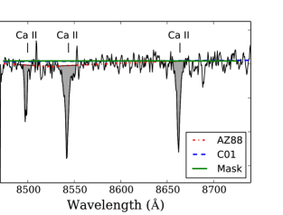
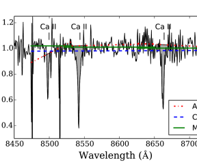
Figure 1: Continuum fits with the AZ88 (dot-dashed red lines) and C01 continuum definitions (dashed blue lines) compared to the continuum fitting with masked out regions (sold green lines). Two GCs are shown: the metal rich GC B163 (left) and the lower S/N, more metal poor GC, H23 (right). Note that in the left figure the C01 continuum definition is identical to the masked fits. The C01 definitions and the masked regions provide better estimates of the continuum for metal rich GCs, though the C01 definitions may be more sensitive to noise and sky lines in lower quality spectra.

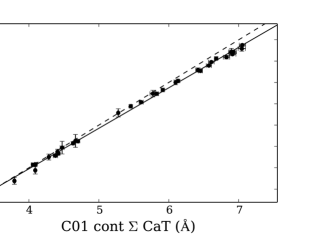
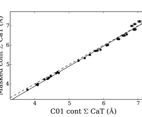
Figure 2: Comparisons between measurements of the IL CaT strength in the template-fitted spectra with different continuum definitions. In every case the line definitions of AZ88 are adopted, with varying continuum fits. Left: The AZ88 vs. C01 continuum definitions. Right: Averaged continuum fits to the observed data with sky lines and known atomic lines masked out, versus the C01 continuum definitions. The points are the M31 GCs. The dashed line shows equal values, while the solid black line shows a least squares fit.

3.2 Line Strengths

Measuring the strength of the CaT lines is a nontrivial process because the lines are strong (i.e. saturated) and may be blended with other features. As discussed earlier, the original AZ88 calibration utilized “pseudo equivalent widths” (EWs), which measure the area within a defined region. Individual stellar analyses (e.g. Battaglia et al. 2008) often fit Gaussian profiles to the spectral lines—however, the CaT lines have strong Lorentzian wings and are distinctly non-Gaussian. Battaglia et al. (2008) compensate for the wings by adding some factor to their Gaussian EWs; however the lines can also be fit with Voigt profiles. All these options are explored to identify the ideal option for the current calibration and for future extragalactic studies.

The extragalactic analyses of Foster et al. (2010) and Usher et al. (2012) use template fits to their (often low S/N) spectra. Although template fits are not strictly necessary for these M31 GCs, they do help reduce scatter in plots; the observed spectra and the template fits are therefore considered for the tests below.

3.2.1 Template fits

Though the CaT lines in the observed M31 spectra can be easily measured, this is not feasible for more distant systems where the S/N is much lower. Foster et al. (2010) and Usher et al. (2012) combat this problem by fitting the observed spectra with a combination of stellar templates, which include 11 giants and 2 dwarfs of a range of metallicities and temperatures. For the APO targets sixteen stellar templates are utilized, encompassing a wide range in metallicity (from [Fe/H]$\sim-2$ to $0$), surface gravity, and effective temperature; for the KPNO targets only ten stellar templates were observed, with a similar range in parameters. All the template stars were selected to be stars that could be found in GCs; in particular, several horizontal branch stars were observed, including a very blue one.

As in Foster et al. (2010) and Usher et al. (2012), the penalized pixel-fitting (pPXF) code of Cappellari & Emsellem (2004) was used to find the linear combination of stellar templates that best fits a given observed spectrum. The templates were fit over the $8440-8820$ Å  region for the KPNO/WIYN spectra and the $8440-8950$ Å  region for the DIS spectra. Sample template fits to B088 and PA56 are shown in Figure 3. Even lower S/N clusters with strong residual sky line contamination (such as PA56) are reasonably well fit by the templates. Several clusters, including B088, are best fit with a small contribution from the hottest blue horizontal branch star, which leads to very weak Paschen lines in the fitted spectra (which was also seen in the stacked spectra from Usher et al. 2015). These Paschen lines do not have a strong effect on the CaT line strengths. Errors in the template fits were estimated with Monte Carlo resampling of the observed spectra one hundred times.

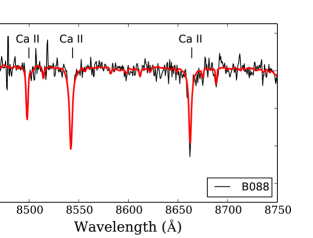
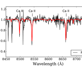
Figure 3: Template fits (red) to the observed B088 and PA56 spectra (black). The three CaT lines are indicated.

3.2.2 Line Integrations in Observed Spectra

Again, the indexf program (Cardiel, 2010) was used to measure pseudo EWs and their associated errors. Given the results in Section 3.1 the C01 continuum definitions are adopted. The AZ88 and C01 line definitions are considered; the C01 definitions are slightly wider than the AZ88 ones, and are likely to cover the wings of the lines more fully (especially for GCs with large velocity dispersions). This measurement technique works well for spectra of bright targets that are not significantly affected by sky line residuals. Many of these M31 GC spectra, however, are affected by sky lines, which will a) systematically affect the measurements of the CaT lines and b) add scatter to any correlation with [Fe/H]. These effects are undesirable for a test of the correlation with [Fe/H], and comparisons are only performed on the template-fitted spectra. Figure 4 compares measurements with the C01 and AZ88 definitions, both using the C01 continuum definitions. Because the C01 indices are wider than the AZ88 indices they are stronger, with the offset increasing with CaT strength. The C01 line definitions are utilized in all subsequent integrations; note that the fit in Figure 4 can be used to convert AZ88 definitions to C01 definitions.

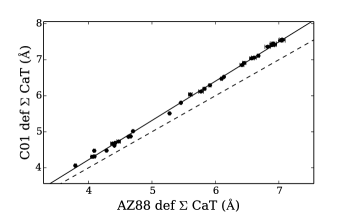
Figure 4: Measurements with the C01 line definitions compared to the AZ88 definitions. Both measurements utilize the C01 continuum regions.

3.2.3 Gaussian and Voigt Fits

Given noise and possible sky line contamination in the line profiles, it will be more accurate to fit full spectral line profiles than to simply integrate within defined regions. CaT lines are often measured with Gaussians (e.g. Battaglia et al. 2008), but as the CaT lines are very strong, Voigt profiles are more appropriate.

There are a variety of automated line measurement programs. This analysis utilizes the pymodelfit program to measure Gaussian and Voigt profiles. Insufficiently removed sky lines are assigned low weights to prevent them from affecting the line profiles. Sample fits to the third CaT line are shown in Figure 5 for GCs with moderate and low S/N and some amount of skyline contamination. Errors in the fits and resulting line strengths are determined by resampling the spectra 100 times with Monte Carlo sampling and bootstrapping. Note that the continuum level is fit during the original profile measurement with sky lines and atomic lines masked out (see Section 3.1), but is not remeasured during the resampling.

Comparisons with the pseudo EWs from Section 3.2.2 are shown in Figure 6. Significant outliers are labelled; these are the lower S/N GCs with strong sky contamination that has affected the pseudo EW measurements. It is apparent that the Gaussian fits underpredict the strengths of the CaT, likely because the strong Lorentzian wings are not included. The Voigt profiles match the pseudo EWs for weak CaT strengths; as the CaT lines strengthen, however, the Voigt profiles become stronger than the pseudo EWs. This may be partly due to continuum offsets (see Figure 2). The scatter is still relatively large because of noise and residual sky lines, and a comparison with the template-fitted spectra may be more appropriate.

Figure 7 compares the Voigt profile fits on the observed and template-fitted spectra, demonstrating that the agreement is generally good, with the exception of the low S/N GCs with strong sky line contamination. In the latter case, full template fits may outperform fits of individual lines in the observed spectra. Figure 7 then compares Voigt profile fits to integrations with the C01 indices, both on the template-fitted spectra. There is a slight offset that increases with CaT strength—again, this may be partly due to continuum effects (Figure 2), but is primarily driven by differences in the line measurements.

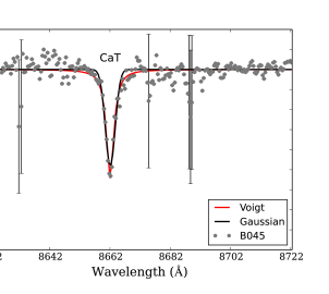
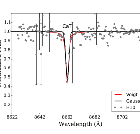
Figure 5: Sample Gaussian and Voigt profile fits to the third CaT line (at 8662 Å) in B045 (left) and H10 (right). The grey points show the data while the black and red lines show the Gaussian and Voigt profile fits, respectively. H10 has lower S/N and a greater contamination from sky emission lines; as a result H10’s EW uncertainties are higher than B045’s.

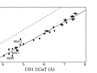
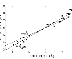
Figure 6: Comparisons between measurements of the IL CaT strength in the observed (not template-fitted) spectra. The points shows individual GCs and the $1\sigma$ errors. The dashed line shows perfect agreement, while the solid line shows a linear least squares fit. Left: Measurements with the C01 definitions (see Section 3.2.2) versus Gaussian fits to the three CaT lines. Right: Measurements with C01 definitions versus Voigt fits.

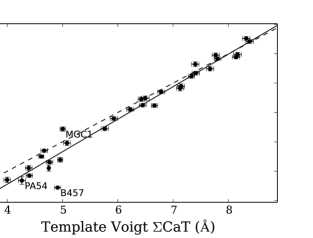
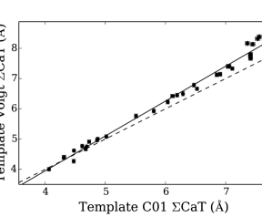
Figure 7: Comparisons between measurements of the IL CaT strength in the template spectra. Points are as in Figure 6. Left: Voigt fits on the raw spectra versus the template spectra. Right: Voigt fits on the template spectra versus pseudo EWs on the template spectra with the Cenarro et al. (2001) definitions.

4 CaT strength and Metallicity

Section 3 demonstrated that there are two ideal ways to accurately measure IL CaT strengths over a wide metallicity range: 1) integrations of line profiles in template-fitted spectra with the C01 line and continuum definitions and 2) Voigt profile fits to observed or template-fitted spectra (though note that Voigt profile fits on observed spectra may not be ideal for distant, fainter clusters). With these measurements the relationship between total CaT strength and [Fe/H] can be determined. Because of the disagreement in radial velocity (see Section 2.4), B457 has been removed from these fits.

The high resolution [Fe/H] ratios versus CaT strengths are shown in Figure 8. The relationship between CaT strength and [Fe/H] was assumed to follow a piecewise linear function, in order to account for possible changes in the slope (see Section 4.1). The optimal slopes, intercepts, and the breakpoint were found with the SciPy (Jones et al., 2001) optimize.curve_fit() package. These piecewise linear fits were initialized with a least-squares linear fit to the full dataset, and with an assumed breakpoint at $[\rm{Fe/H}]\sim-0.8$. The fits are mildly sensitive to the initial slope, but are less sensitive to the initial breakpoint. Note that the relationship for Voigt profile fits is very similar between the observed and template-fitted spectra. Two separate fits were done for each measurement technique: one utilizing all GCs and another without the most metal rich GC B193 or the metal poor, low [$\alpha$/Fe] clusters (G002, MGC1, PA17, PA53; see Sections 4.1 and 4.2).

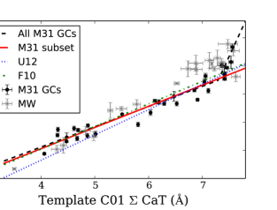
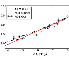
Figure 8: High resolution [Fe/H] versus integrated CaT strength in the template-fitted spectra, utilizing the C01 definitions (left) and Voigt profile fits (right). The black circles show the M31 clusters. The dashed black lines show the piecewise linear fits to all M31 GCs; the solid red lines show fits without the metal rich GC B193 (see Section 4.1) or the low [Ca/Fe] GCs (see Section 4.2). The grey crosses show the MW clusters from AZ88. The green dot-dashed line shows the fit from Foster et al. (2010), while the dotted blue line shows the Usher et al. (2012) fit (after converting from [Z/H] to [Fe/H]; see Section 4.3)

.

4.1 Breakpoint in the CaT-Metallicity Relationship

Both measurement techniques show a breakpoint in their CaT-[Fe/H] relations when the most metal cluster, B193, is included in the fit. This breakpoint has been seen in other IL CaT studies. Vazdekis et al. (2003) found evidence of a breakpoint in their models of the CaT, while Foster et al. (2010) saw evidence of a turnover in their empirical calibration with NGC 1407 GCs. These studies referred to this turnover as a “saturation” point, which is a misnomer since the CaT lines are saturated in all the target GCs (that is, the lines lie on the nonlinear part of the curve of growth). In measurements of the CaT strengths in GCs associated with early type galaxies, Usher et al. (2012) find no evidence for a breakpoint. They attribute this to their continuum fits, which rely on areas that are relatively free of weaker atomic lines (much like the continuum regions defined by C01; see Section 3.1). The lack of a breakpoint for the C01 pseudo EWs and the Voigt profiles (when B193 is removed) supports the idea that the breakpoint is caused by line blanketing in the continuum regions. Since neither continuum fitting technique can adequately fit B193, this suggests that the CaT strength-[Fe/H] may become uncertain above $[\rm{Fe/H}]\sim-0.4$.

It is important to note that continuum fits become increasingly difficult as a GC’s metallicity increases. Not only do atomic lines become stronger, molecular lines become increasingly important as well. Metal rich GCs are also likely to host cool M giants with strong TiO absorption in the CaT region; in IL spectra M giants may have a non-negligible contribution to the CaT region. Their molecular lines will likely affect the continuum and the lines themselves, and may be difficult to detect. The CaT lines in B193 ($[\rm{Fe/H}]\sim-0.2$) may be affected by molecular line blanketing, leading to weaker measured CaT lines with all measurement techniques. This is demonstrated in Figure 9, which shows the CaT spectra of B193 and an M8 metal rich AGB star. The red dashed lines show the strongest TiO bandheads (also see Figure 1 in C01). B193 seems to have some moderate absorption at 8860 Å, which implies that there will be weak TiO absorption throughout the CaT region. TiO absorption was also seen in the stacked red (metal rich) spectra from Usher et al. (2015). The numbers of M giants in metal rich GCs (and their precise temperatures) is likely to be somewhat stochastic; as a result, TiO blanketing may lead to scatter in the [Fe/H]-CaT relation at high [Fe/H].

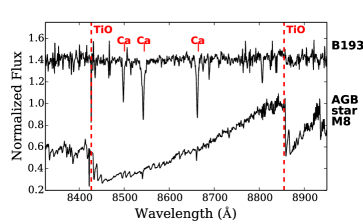
Figure 9: The IL CaT spectrum of the metal rich GC B193, along with a spectrum of an M8 AGB star. The cool AGB star’s spectrum is dominated by TiO bands; the two strongest bandheads at 8432 and 8860 Å  are indicated with red dashed lines. The 8860 Å  feature is also detectable in the B193 spectrum, which hints that the CaT features may also be affected by TiO absorption from M giants in the cluster.

4.2 The Effects of Detailed Chemical Abundances

The CaT lines are sensitive to the electron pressure in stellar atmospheres; nonstandard chemical abundance mixtures may affect the measured CaT strength and the inferred [Fe/H]. A handful of GCs in this sample are chemically distinct from typical MW and M31 GCs—that is they have abundance ratios that indicate they may have formed in dwarf galaxies that were later accreted by M31. One of the most telling signs of accretion is a low [Ca/Fe] ratio at a given [Fe/H]. In addition, several of these chemically anomalous GCs are located on or near stellar streams, with radial velocities that link them to the streams and/or to each other (Veljanoski et al., 2014). The clusters that are likely associated with stellar streams include H10, PA53, and PA56, while the chemically peculiar GCs (in more than one abundance ratio) without a known stream or host galaxy include G002, MGC1, and PA17.

Figure 10 shows the offsets from the CaT strength-metallicity relation for the Voigt profile fits to template-fitted spectra versus [Ca/H], with the chemically interesting GCs indicated with red stars. [Ca/H] is utilized rather than [Ca/Fe], since the metal rich GCs also have lower [Ca/Fe] ratios (due to standard chemical evolution; see Tolstoy et al. 2009). To separate chemical abundance offsets from continuum issues, [Ca/H] is used instead of [Ca/Fe]. B193 clearly sticks out at the metal rich end (see Section 4.1). Only the fits with the low [Ca/Fe] GCs (and B193) excluded from the fit is shown. Though there is no definite trend in Figure 10, the metal poor, chemically peculiar GCs stand out, with their CaT strengths systematically lower than the “normal” GCs. This indicates that a GC’s detailed abundances can affect its CaT line strengths, particularly at the metal poor end. For this reason, the best CaT strength-metallicity relations are determined without these GCs.

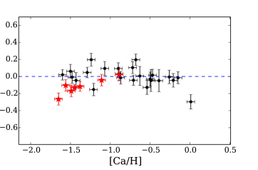
Figure 10: Offsets from the best fitting CaT strength-metallicity relationship versus [Ca/H] when the chemically peculiar GCs are excluded from the fit. The GCs with low [Ca/Fe], other abundance ratios, and/or locations along stellar streams that indicate they may have formed in dwarf galaxies are indicated with red stars; these GCs are G002, MGC1, H10, PA17, PA53, and PA56.

4.3 Comparisons with Previous Results

Empirical relationships between integrated CaT strength and GC metallicity have been determined in three major studies: the original Galactic GC calibration by AZ88, the recalibration of the AZ88 relation by Foster et al. (2010), and the SSP-based calibration of Usher et al. (2012). These papers all used slightly different methods to determine CaT strengths, and are discussed individually.

4.3.1 AZ88’s Original Calibration: Milky Way GCs

The CaT strengths from AZ88 and the high resolution [Fe/H] ratios can be directly compared to those of the M31 GCs. The MW CaT lines were measured with the AZ88 line definitions and continuum regions. Sections 3.1 and 3.2.2 demonstrated that there is a clear offset between pseudo EWs measured with the AZ88 vs. C01 definitions. This offset has been applied to adjust the MW CaT strengths, and the MW GCs are shown in Figure 8. The adopted metallicities for the Galactic GCs are from Harris (1996, 2010 edition), to ensure that the MW GCs are on the same [Fe/H] scale; the Harris metallicities are from compilations of high resolution analyses of individual stars, and should roughly match the high resolution metallicities from Colucci et al. (2014) and Sakari et al. (2015, 2016 in prep.). For 47 Tuc and M15 the IL [Fe/H] ratios from Sakari et al. (2013) are adopted.

The MW GCs are slightly offset from the M31 GCs, particularly at intermediate metallicities. This may be due to metallicity offsets. However, it may also be an effect of spectral resolution. The AZ88 measurements were made on lower resolution spectra ($R\sim 2000$); the resulting blending may make continuum levels even more difficult to identify. As a result, the breakpoint in the relation may come at a lower metallicity than the M31 GCs. Regardless of the cause, the MW GCs generally agree with the M31 GCs.

4.3.2 The Foster et al. (2010) Rederivation of AZ88

Foster et al. (2010) rederived the AZ88 CaT strength-[Fe/H] relationship with the same line definitions but with better continuum fitting, ensuring better performance at high metallicity. The Foster et al. relation was shifted to the wider C01 line definition (see Section 3.2.2), and is also shown in Figure 8. The agreement with the M31 GC relation is excellent; the relations start to diverge slightly at the metal rich end, though the difference is not significant.

4.3.3 The Usher et al. (2012) SSP-based Relation

Usher et al. (2012) present two CaT-metallicity calibrations: a rederivation of the Foster et al. relation and a new calibration based on SSP models. As Usher et al. select the latter relation as the better choice, only the SSP-based model is considered here. As with Foster et al. (2010), Usher et al. use the AZ88 line definition but perform more robust continuum identifications; their relation has therefore also been shifted to the C01 line definitions (see Section 3.2.2). However, their relation is given in [Z/H] rather than [Fe/H]. It is difficult to know how to compare theoretical total metallicities to spectroscopic [Fe/H] ratios. In principle there are two approaches.

1. Convert GC [Fe/H] ratios to [Z/H] using detailed abundances. In practice this approach is extremely difficult, since large star-to-star variations exist within GCs, in some of the most abundant elements (e.g. He, C, N, O, Na, Mg, Al) due to evolutionary and/or GC processes (e.g. Gratton et al. 2000; Briley et al. 2004; Carretta et al. 2009a). This is further complicated by potentially large systematic errors which may plague observed abundance ratios (Sakari et al., 2014). Finally, the SSP models do not account for light element variations, and this is likely to not be a robust way to compare the two relations.

2. Convert SSP [Z/H] ratios to [Fe/H]. In principle this approach should be simpler than converting observationally-determined abundance ratios, since the inputs to the model are known. However, the precise abundance mixture and the metallicity scale will affect the final [Z/H]. This is the method that is adopted for this comparison.

Usher et al. adopted solar-scaled SSPs and then adjusted those values to account for varying [$\alpha$/Fe], following the prescription of Mendel et al. (2007). To compare with the M31 GCs, these [Z/H] ratios were then converted to the Harris et al. (1996, 2003 edition) utilizing Usher et al.’s Equation 3. Technically, their Equation 3 was determined for a different set of SSP models than was used for their final CaT strength-metallicity relationship; however, their [$\alpha$/Fe] correction should correct for any offset. The converted relationship is shown in Figure 8.

The metallicity scale is very important for this conversion. Usher et al. also provide a calibration on the Carretta et al. (2009b) scale, which leads to a more discrepant slope from the M31 GCs. Undoing the Mendel et al. (2007) correction leads to a large offset, which indicates that some adjustment to a metallicity scale is necessary. As with the AZ88 GCs, the Harris metallicity scale is chosen because its [Fe/H] ratios come primarily from high resolution, individual stellar spectroscopy, and should provide the best agreement with the M31 literature values. Even with the Harris metallicity scale, there is some evidence for a slope difference. This could indicate further problems in the metallicity scale, or it could indicate problems with the Usher et al. scale at low [Fe/H].

4.4 Paschen Lines

The template-fitted M31 spectra of the metal poor GCs show slight Paschen features. Usher et al. (2015) also detected weak Paschen lines in their stacked spectra of blue (metal poor) GCs. These weak Paschen lines do not have a significant affect on the CaT strengths in these GCs, which are all older than $\sim 2$ Gyr. However, they may be significant in younger clusters. C01 define a CaT* index that accounts for nearby Paschen lines. This index seems to overcorrect the CaT strengths in these old M31 GCs, but may be essential for young clusters.

4.5 Versions of CaT Strength

Various studies have utilized different combinations of the CaT lines. For future studies of more distant clusters, it may be desirable to utilize different combinations of lines; for instance, the first CaT line may be too weak to detect confidently or the third CaT line may be completely obscured by sky lines. For this reason, Table 2 presents the CaT strength-metallicity relationships for different combinations of the CaT lines. Three different combinations are considered: the classic sum of all three CaT lines, the sum of the strongest two (the second and third; e.g. Tolstoy et al. 2001), and the second CaT line by itself. Naturally the relation for the second CaT line is more uncertain than the others. The slope of the CaT2$+$CaT3 relation is also slightly steeper than the relation with all three lines.

Note that when Paschen contamination is significant (e.g. for younger GCs), the first CaT line may be more reliable for measuring GC metallicity (Wallerstein et al., 2012). Given that the first CaT line is weaker, the errors on this relationship are larger, and this relation is not included in Table 2.

Given that the derived relations are very sensitive to the measurement techniques, the M31 CaT spectra from this paper are available online.

Table 2: CaT strength vs. metallicity relationships, for different indicators of the CaT strength.

Measurement	CaT Strength	Relation
Technique	Indicator
Pseudo EWs (C01 definitions)	$\Sigma$CaT	$[\rm{Fe/H}]=(0.38\pm 0.10)\times\rm{CaT}-(3.48\pm 0.13)$
	CaT2 + CaT3	$[\rm{Fe/H}]=(0.45\pm 0.10)\times\rm{CaT}-(3.45\pm 0.20)$
	CaT2	$[\rm{Fe/H}]=(0.78\pm 0.20)\times\rm{CaT}-(3.36\pm 0.33)$
Voigt Profile Fits	$\Sigma$CaT	$[\rm{Fe/H}]=(0.36\pm 0.10)\times\rm{CaT}-(3.49\pm 0.20)$
	CaT2 + CaT3	$[\rm{Fe/H}]=(0.44\pm 0.20)\times\rm{CaT}-(3.49\pm 0.19)$
	CaT2	$[\rm{Fe/H}]=(0.74\pm 0.40)\times\rm{CaT}-(3.32\pm 0.50)$

4.6 Age Effects

Figure 11 shows offsets from the CaT strength-metallicity relationship versus GC age, where the ages are from the high resolution spectroscopic analyses of Colucci et al. (2014) and Sakari et al. (2015, 2016 in prep.). Down to $\sim 2$ Gyr, there is no significant trend, suggesting that age has little effect on the IL CaT (although the large error bars on the age prohibit any subtle trend from being detected). This may not be true for younger GCs if strong Paschen lines begin to contaminate the CaT lines and continuum regions; in that case the C01 CaT* index may help to remove Paschen contamination.

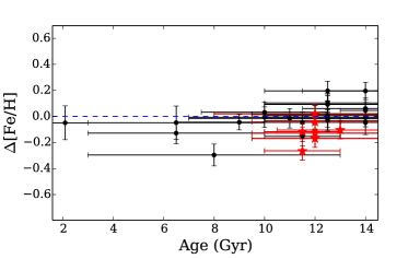
Figure 11: Offsets from the best fitting CaT strength-metallicity relationship versus age. Points are as in Figure 10. There is no significant relationship between GC age and offset from the best-fitting CaT strength-metallicity relation.

5 Discussion: Interpretations of CaT Strengths

Considered as a whole, the tests with these well-studied, relatively nearby M31 GCs have reproduced the indirect calibrations of Foster et al. (2010) and Usher et al. (2012), at least for the observed metallicity range. However, these tests have also shown that CaT measurements are not trivial, particularly for metal rich GCs with significant line blanketing. This line blanketing makes it difficult to identify continuum levels, and will become even worse with large velocity dispersions. Nonstandard chemical abundance mixtures (e.g. for GCs that appear to have formed in dwarf galaxies) also confuse the CaT relation at the low metallicity end. Foster et al. (2010) and Usher et al. (2012) found several intriguing inconsistencies between CaT and colour-based metallicities, which they have attributed to continuum problems and age or chemical abundance differences. With this set of nearby M31 GCs, which have been well studied, these hypotheses can start to be tested.

5.1 Metallicity Bimodalities

In their study of NGC 1407, Foster et al. (2010) found that the general shape of the CaT bimodality (which was only detected in template-fitted spectra) did not match the shape of the colour bimodality. Foster et al. (2011) also noted an excess of GCs in NGC 4494 at $[\rm{Fe/H}]=-0.9$ (determined with their CaT calibration), which corresponds to a trough in the colour distribution. B193’s large offset from the best-fitting relation suggests that Foster et al.’s distribution was affected by line blanketing in the most metal rich GCs, which led to continuum issues and subsequent weakening of the measured CaT lines. If the best-fitting relation in this paper were applied to GCs at B193’s metallicity, they would also seem to pile up at lower metallicities, weakening any intrinsic bimodality with a significant metal rich population. Though this problem may be alleviated with more rigorous continuum fits, it is likely to remain a difficulty for metal rich GCs.

5.2 The Blue Tilt

The blue tilt is a photometric phenomenon where the brightest GCs in the blue (metal poor) subpopulation appear redder than their fainter counterparts. There has also been weak photometric evidence for inverse red tilts (Harris 2009) and positive red tilts (Mieske et al., 2010), although neither case is very significant. These tilts have been attributed to abundance variations within the most massive GCs, a hypothesis that is borne out by observations of some MW GCs, e.g. NGC 1851 (e.g. Carretta et al. 2010), NGC 3201 (Hughes et al. 2015, in prep.), and $\omega$ Cen (e.g. Johnson & Pilachowski 2010), which have large spreads in many elements, including heavy elements like Fe. Even monometallic GCs like M15 show large star-to-star variations in Mg, which could affect its integrated colours (e.g. Sneden et al. 1997).

Foster et al. (2010) found that the brightest GCs in both subpopulations have identical CaT strengths, leading to identical CaT-based metallicities despite being well separated in colour. Usher et al. (2012) confirmed this result. Possible explanations for this behaviour included non universal colour-CaT strength relations and chemical or age differences between GC populations. However, it is also possible that the CaT strengths of the brightest metal rich GCs could be systematically underpredicted because of continuum uncertainties. If the brighter GCs are more massive, they will have higher velocity dispersions, leading to more blending of the atomic features—such an effect would also be seen at lower spectral resolution (e.g. with the MW GCs; see Section 4.3). C01 and Vazdekis et al. (2003) explored velocity dispersion and resolution effects and concluded that the strengths of the C01 indices were unaffected by broadening, up to large velocity dispersions. However, the continuum levels are likely to be affected, which may be difficult to detect in low S/N spectra. Similarly, narrow line definitions will be affected by line broadening; while the C01 indices are unaffected, the AZ88 definitions may be affected by velocity dispersion. Continuum offsets at a fixed metallicity with increasing cluster mass would indeed be detectable as a negative tilt in the metal rich GCs. Usher et al. (2015) find no evidence for a red tilt in their stacked spectra.

Thus, while the blue tilt could indeed be a result of multiple populations within GCs, a red tilt could be created (or exaggerated) by systematic offsets between massive and low mass GCs at the same metallicity. This could also lead to observational biases when observing faint GC systems where only the most massive GCs are observable.

The tests in Section 4.2 also demonstrated that the detailed abundance mixture does affect the CaT strength and the inferred metallicity. None of the chemically peculiar GCs investigated here are massive enough to create a blue tilt, but the most massive, metal poor GCs are likely to have strong star-to-star variations in elements that could complicate interpretations of the CaT strength (e.g. Mg; Carretta et al. 2009a).

5.3 CaT Metallicity-Colour Relationships

The most intriguing result from the Usher et al. (2012) analysis is that the CaT metallicity-colour relationship does not seem to be the same for all galaxies. In particular, while there is excellent agreement between GCs at intermediate metallicities in all galaxies, certain galaxies have large discrepancies at high or low metallicity. By stacking spectra from GCs with similar colours, Usher et al. (2015) confirmed these CaT-colour differences between early-type galaxies. These differences are driven mostly at the metal rich end, though at the metal poor end differences are seen between galaxies with luminous vs. faint GC systems. Most of the GCs are quite bright, and are therefore likely to be massive.

The results from this paper suggest that care should be taken at the metal rich end. Although Usher et al. (2015) argue that there is no evidence for a red tilt in their stacked spectra (i.e. the CaT strength does not depend on GC magnitude), stochastic effects (e.g. the numbers of cool M giants) in metal rich GC populations could lead to a spread in the CaT strength-metallicity relationship. Fe spreads in the most massive GCs could also confuse CaT-colour relationships.

At the metal poor end, detailed chemical abundances can affect the slope of the CaT-[Fe/H] relationship. GCs that formed in dwarf galaxies and have primordial abundance differences from MW and M31 stars and GCs have lower predicted [Fe/H] ratios at a given CaT strength. While it is unlikely that the early type galaxies host significant populations of dwarf galaxy clusters, they almost certainly host variations in He, C, N, O, Na, Mg, and/or Al. Usher et al. (2015) propose that these variations would lead to colour differences, but they may also lead to differences in CaT strength. With these chemical variations it is difficult to interpret a GC’s total metallicity.

The takeaway message from this M31 GC analysis is therefore one of caution: CaT-based metallicities are highly sensitive to measurement techniques, and are likely to become increasingly difficult with higher [Fe/H] and velocity dispersion.

6 Conclusion

This paper has presented the first comparison between integrated CaT measurements and high resolution integrated [Fe/H] since the original Armandroff & Zinn (1988) analysis. The M31 GCs used for this analysis span a wide metallicity range, from $[\rm{Fe/H}]~{}=~{}-2$ to $-0.2$, and cover ages from $\sim 2-14$ Gyr. The results from Sections 3 and 4 demonstrate several crucial aspects of the CaT as a metallicity indicator.

1. The quantitative strength of the CaT lines depends on the measurement techniques. Voigt profiles best fit the lines, though line integrations also work, provided that the line bandpasses are defined appropriately.

2. Template fits to the observed spectra do not introduce significant systematic offsets in the measured CaT strengths, provided that the templates cover a sufficient range in parameter space.

3. The CaT line strengths are significantly affected by continuum fits. Continuum fits that rely on continuum bandpasses (such as the AZ88 definitions) will be blanketed by atomic lines in GCs with $[\rm{Fe/H}]\ga-1$. The most metal rich GCs may have strong molecular features that are contributed by cool M giants; this contamination may be seen in the TiO bandhead at 8860 Å. It is extremely difficult to fit continuum levels properly in these most metal rich clusters. Similarly, high velocity dispersion GCs will have atomic lines blended together, further complicating continuum estimates.

4. If continuum levels are properly fit the integrated CaT is an excellent [Fe/H] indicator, to within $\sim 0.2$ dex. The precise relationship depends mildly on the techniques used to the measure the line strengths and on the specific lines used.

5. Age does not affect the CaT line strengths in any of these clusters, which are older than $\sim 2$ Gyr.

6. Detailed abundance mixtures may also play a small role in the derived [Fe/H].

Interpretations of CaT-based metallicities must consider the difficulties in accurately measuring CaT strength, the potential biases that may occur from only observing the brightest GCs, and any additional systematic effects that could alter the integrated CaT strength.

References

- Armandroff & Zinn (1988) Armandroff, T.E. & Zinn, R. 1988, AJ, 96, 92
- Battaglia et al. (2008) Battaglia, G., Irwin, M., Tolstoy, E., et al. 2008, MNRAS, 383, 183
- Bershady et al. (2004) Bershady, M.A., Andersen, D.R., Harker, J., Ramsey, L.W., & Verheijen, M.A.W. 2004, PASP, 116, 565
- Bershady et al. (2005) Bershady, M.A., Andersen, D.R., Verheijen, M.A.W., Westfall, K.B., Crawford, S.M., & Swaters, R.A. 2005, ApJS, 156, 311
- Bershady et al. (2008) Bershady, M., Barden, S., Blanche, P.-A., et al. 2008, Society of Photo-Optical Instrumentation Engineers (SPIE) Conference Series, 7014
- Briley et al. (2004) Briley, M.M., Harbeck, D., Smith, G.H., & Grebel, E.K. 2004, AJ, 127, 1588
- Brodie & Strader (2006) Brodie, J.P. & Strader, J. 2006, ARA&A, 44, 193
- Caldwell et al. (2011) Caldwell, N., Schiavon, R., Morrison, H., Rose, J.A., & Harding, P. 2011, AJ, 141, 18
- Cappellari & Emsellem (2004) Cappellari, M. & Emsellem, E. 2004, PASP, 116, 138
- Cardiel (2010) Cardiel, N. 2010, Astrophysics Source Code Library
- Carretta et al. (2009a) Carretta, E., Bragaglia, A., Gratton, R., & Lucatello, S. 2009a, A&A, 505, 139
- Carretta et al. (2009b) Carretta, E., Bragaglia, A., Gratton, R., D’Orazi, V., & Lucatello, S. 2009b, A&A, 508, 695
- Carretta et al. (2010) Carretta, E., Gratton, R.G., Lucatello, S., et al. 2010, ApJ, 722, L1
- Cenarro et al. (2001) Cenarro, A.J., Cardiel, N., Gorgas, J., Peletier, R.F., Vazdekis, A., & Prada, F. 2001, MNRAS, 326, 959
- Colucci et al. (2009) Colucci, J.E., Bernstein, R.A., Cameron, S., McWilliam, A., & Cohen, J.G. 2009, ApJ, 704, 385
- Colucci et al. (2011a) Colucci, J.E., Bernstein, R.A., Cameron, S.A., & McWilliam, A. 2011, ApJ, 735, 55
- Colucci et al. (2011b) Colucci, J.E. & Bernstein, R.A. 2011, EAS Pub. Ser., 48, 275
- Colucci et al. (2012) Colucci, J.E., Bernstein, R.A., Cameron, S.A., & McWilliam, A. 2012, ApJ, 746, 29
- Colucci et al. (2013) Colucci, J.E., Duran, M.F., Bernstein, R.A., & McWilliam, A. 2013, ApJ, 773, 36
- Colucci et al. (2014) Colucci, J.E., Bernstein, R.A., & Cohen, J.G. 2014, ApJ, 797, 116
- Conroy & van Dokkum (2012) Conroy, C. & van Dokkum, P.G. 2012, ApJ, 760, 71
- Ferreras et al. (2013) Ferreras, I., La Barbera, F., de la Rosa, I.G., et al. 2013, MNRAS, 429, 15
- Foster et al. (2010) Foster, C., Forbes, D.A., Proctor, R.N., Strader, J., Brodie, J.P., & Spitler, L.R. 2010, AJ, 139, 1566
- Foster et al. (2011) Foster, C., Spitler, L.R., Romanowsky, A.J., et al. 2011, MNRAS, 415, 3393
- Galleti et al. (2004) Galleti, S., Federici, L., Bellazzini, M., Fusi Pecci, F., & Macrina, S. 2004, A&A, 416, 917
- Galleti et al. (2006) Galleti, S., Federici, L., Bellazzini, M., Buzzoni, A., & Fusi Pecci, F. 2006, A&A, 456, 985
- Gratton et al. (2000) Gratton, R.G., Sneden, C., Carretta, E., & Bragaglia, A. 2000, A&A, 354, 169
- Harris (1996, 2010 edition) Harris, W.E. 1996 (2010 edition), AJ, 112, 1487
- Harris (2009) Harris, W.E. 2009, ApJ, 699, 254
- Harris et al. (2013) Harris, W.E., Harris, G.L.H., & Alessi, M. 2013, ApJ, 772, 82
- Hinkle (2003) Hinkle, K., Wallace, L., Livingston, W., Ayres, T., Harmer, D., & Valenti, J. 2003, in The Future of Cool-Star Astrophysics: 12th Cambridge Workshop on Cool Stars, Stellar Systems, and the Sun (2001 July 30 - August 3), eds. A. Brown, G.M. Harper, and T.R. Ayres, (University of Colorado), 851
- Huxor et al. (2014) Huxor, A.P., Mackey, A.D., Ferguson, A.M.N., et al. 2014, MNRAS, 442, 2165
- Johnson & Pilachowski (2010) Johnson, C.I. & Pilachowski, C.A. 2010, ApJ, 722, 1373
- Jones et al. (2001) Jones, E., Oliphant, E., Peterson, P., et al. 2001, http://www.scipy.org
- Knezek et al. (2010) Knezek, P.M., Bershady, M.A., Willmarth, D., et al. 2010, Society of Photo-Optical Instrumentation Engineers (SPIE) Conference Series, 7735
- McWilliam & Bernstein (2008) McWilliam, A. & Bernstein, R. 2008, ApJ, 684, 326
- Mendel et al. (2007) Mendel, J.T., Proctor, R.N., & Forbes, D.A. 2007, MNRAS, 379, 1618
- Mieske et al. (2010) Mieske, S., Jordán, A., Côté, P., et al. 2010, ApJ, 710, 1672
- Minkowski (1942) Minkowski, R. 1942, ApJ, 96, 306
- Peng et al. (2006) Peng, E.W., Jordán, A., Côté, P. et al. 2006, ApJ, 639, 95
- Sakari et al. (2013) Sakari, C.M., Shetrone, M., Venn, K., McWilliam, A., & Dotter, A. 2013, MNRAS, 434, 358
- Sakari et al. (2014) Sakari, C.M., Venn, K., Shetrone, M., Dotter, A., & Mackey, D. 2014, MNRAS, 443, 2285
- Sakari et al. (2015) Sakari, C.M., Venn, K.A., Mackey, A.D., Shetrone, M.D., Dotter, A., Ferguson, A.M.N., & Huxor, A. 2015, MNRAS, 448, 1314
- Sneden et al. (1997) Sneden, C., Kraft, R.P., Shetrone, M.D., Smith, G.H., Langer, G.E., & Prosser, C.F. 1997, AJ, 114, 1964
- Starkenburg et al. (2010) Starkenburg, E., Hill, V., Tolstoy, E., et al. 2010, A&A, 513, 34
- Tolstoy et al. (2001) Tolstoy, E., Irwin, M.J., Cole, A.A., Pasquini, L., Gilmozzi, R., & Gallagher, J.J. 2001, MNRAS, 327, 918
- Tolstoy et al. (2009) Tolstoy, E., Hill, V., & Tosi, M. 2009, ARA&A, 47, 371
- Trager et al. (2000) Trager, S.C., Faber, S.M., Worthey, G., & González, J.J. 2000, AJ, 119, 1645
- Usher et al. (2012) Usher, C., Forbes, D.A., Brodie, J.P., et al. 2012, MNRAS, 426, 1475
- Usher et al. (2015) Usher, C., Forbes, D.A., Brodie, J.P., et al. 2015, MNRAS, 446, 369
- Vazdekis et al. (2003) Vazdekis, A., Cenarro, A.J., Gorgas, J., Cardiel, N., & Peletier, R.F. 2003, MNRAS, 340, 1317
- Veljanoski et al. (2014) Veljanoski, J., Mackey, A.D., Ferguson, A.M.N., et al. 2014, MNRAS, 442, 2929
- Wallerstein et al. (2012) Wallerstein, G., Gomez, T., & Huang, W. 2012, ApSS, 341, 89
- Worthey et al. (1994) Worthey, G., Faber, S.M., González, J.J., & Burstein, D. 1994, ApJS, 94, 687
- Yoon et al. (2006) Yoon, S.-J., Yi, S.K., & Lee, Y.-W. 2006, Science, 311, 1129