Gaussian Mixture Embeddings for Multiple Word Prototypes

Abstract

Recently, word representation has been increasingly focused on for its excellent properties in representing the word semantics. Previous works mainly suffer from the problem of polysemy phenomenon. To address this problem, most of previous models represent words as multiple distributed vectors. However, it cannot reflect the rich relations between words by representing words as points in the embedded space. In this paper, we propose the Gaussian mixture skip-gram (GMSG) model to learn the Gaussian mixture embeddings for words based on skip-gram framework. Each word can be regarded as a gaussian mixture distribution in the embedded space, and each gaussian component represents a word sense. Since the number of senses varies from word to word, we further propose the Dynamic GMSG (D-GMSG) model by adaptively increasing the sense number of words during training. Experiments on four benchmarks show the effectiveness of our proposed model.

Introduction

Distributed word representation has been studied for a considerable efforts (?; ?; ?; ?; ?; ?; ?; ?; ?; ?). By representing a word in the embedded space, it could address the problem of curse of dimensionality and capture syntactic and semantic properties. In the embedded space, words that have similar syntactic and semantic roles are also close with each other. Thus, distributed word representation is applied to a abundant natural language processing (NLP) tasks (?; ?; ?; ?).

Most of previous models map a word as a single point vector in the embedded space, which surfer from polysemy problems. Concretely, many words have different senses in different contextual surroundings. For instance, word “apple” could mean a kind of fruit when the contextual information implies that the topic of the text is about food. At the meanwhile, the word “apple” could represent the Apple Inc. when the context is about information technology. To address this problem, previous works have gained great success in representing multiple word prototypes. ? (?) constructs multiple high-dimensional vectors for each word. ? (?) learns multiple dense embeddings for each word using global document context. ? (?) proposed multi-sense skip-gram (MSSG) to learn word sense embeddings with online word sense discrimination. Most of previous works are trying to use multiple points to represent the multiple senses of words, which lead to a drawback. It cannot reflect the rich relations between words by simply representing words as points in the embedded space. For instance, we cannot infer that the word “fruit” is the hypernym of the word “apple” by representing these two words as two point vectors in the embedded space.

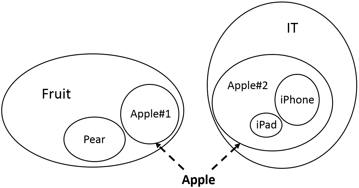
Figure 1: An example of Gaussian mixture embeddings.

In this paper, we propose the Gaussian mixture skip-gram (GMSG) model inspired by ? (?), who maps a word as a gaussian distribution instead of a point vector in the embedded space. GMSG model represents each word as a gaussian mixture distribution in the embedded space. Each gaussian component can be regarded as a sense of a word. Figure 1 gives an illustration of Gaussian mixture embeddings. In this way, much richer relations can be reflected via the relation of two gaussian distributions. For instance, if the word “fruit” has larger variance than the word “apple”, it could show that the word “fruit” is the hypernym of the word “apple”. In addition, using different distance metrics, the relations between words vary. The pair (apple, pear) might be much closer when we use Euclidean distance, while the pair (apple, fruit) might be much closer when we measure them using KL divergence. Further, since the number of senses varies from word to word, we propose the Dynamic GMSG (D-GMSG) model to handle the varying sense number. D-GMSG automatically increases the sense numbers of words during training. Experiments on four benchmarks show the effectiveness of our proposed models.

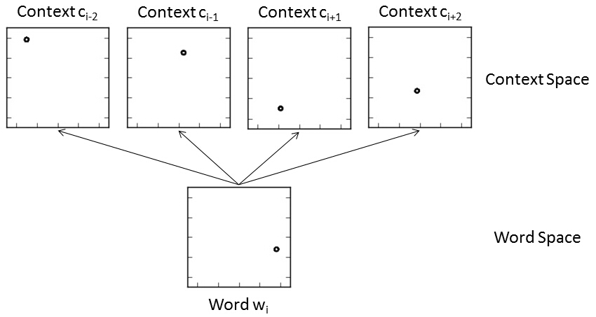
(a) Skip-Gram

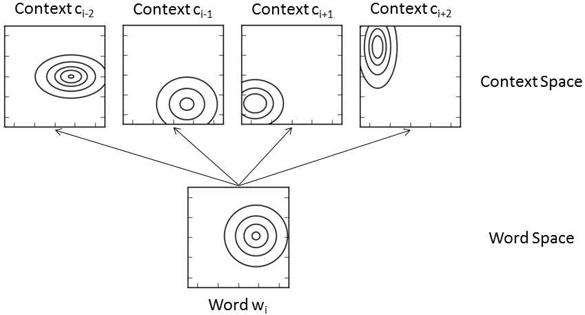
(b) Gaussian Skip-Gram

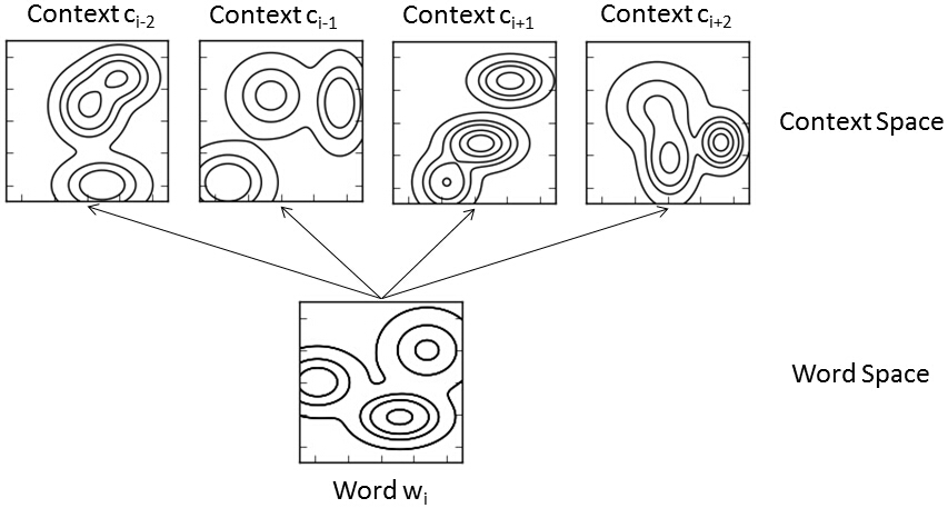
(c) Gaussian Mixture Skip-Gram

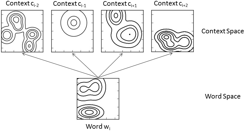
(d) Dynamic Gaussian Mixture Skip-Gram

Figure 2: Four architectures for learning word representations.

Skip-Gram

In the skip-gram model (Figure 2a) (?), each word $w$ is represented as a distributed vector $\mathbf{e}_{w}\in\mathbf{W}$, where $\mathbf{W}\in\mathbb{R}^{|V|*d}$ is the word embedding matrix for all words in word vocabulary $V$. $d$ is the dimensionality of the word embeddings. Correspondingly, each context word $c_{w}$ also has a distributed representation vector $\hat{\mathbf{e}}_{c_{w}}\in\mathbf{C}$, where $\mathbf{C}\in\mathbb{R}^{|V|*d}$ is another distinguished space.

The skip-gram aims to maximize the probability of the co-occurrence of a word $w$ and its context word $c_{w}$, which can be formalized as:

$$\mathbf{v}(w|c_{w})=\prod_{u\in\{w\}\bigcup NEG(w)}p(u|c_{w}),$$ (1)

where function $NEG(\cdot)$ returns a set of negative sampling context words and $p(u|c_{w})$ can be formalized as:

$$p(u|c_{w})=[\sigma(\mathbf{e}_{w}^{\top}\hat{\mathbf{e}}_{u})]^{\textbf{1}\{u=c_{w}\}}[1-\sigma(\mathbf{e}_{w}^{\top}\hat{\mathbf{e}}_{u})]^{\textbf{1}\{u\neq c_{w}\}},$$ (2)

where $\textbf{1}\{\cdot\}$ is a indicator function and $\sigma(\cdot)$ is the sigmoid function.

Given a training corpus $\mathbf{D}$ which insists of $(word,context)$ pairs $(w,c_{w})\in\mathbf{D}$, the goal of skip-gram model is to maximize the objective function:

$$J(\theta)=\sum_{(w,c_{w})\in\mathbf{D}}\log\mathbf{v}(w|c_{w}),$$ (3)

where $\theta$ is the parameter set of the model.

Concretely, the $NEG(w)$ function samples negative contextual words for current word $w$ drawn on the distribution:

$$P(w)\propto P_{unigram}(w)^{sr},$$ (4)

where $P_{unigram}(w)$ is a unigram distribution of words and $sr$ is a hyper-parameter.

Gaussian Skip-Gram Model

Although the skip-gram model is extremely efficient and the learned word embeddings have greet properties on the syntactic and semantic roles, it cannot give the asymmetric distance between words.

Skip-gram model defines the representation of a word as a vector, and defines the similarity of two words $w_{1}$ and $w_{2}$ using cosine distance of vectors $\mathbf{e}_{w_{1}}$ and $\mathbf{e}_{w_{2}}$. Unlike the definition of skip-gram model, in this paper, we argue that a word can be regarded as a function. The similarity between two function $f$ and $g$ can be formalized as:

$$sim(f,g)=\int_{x\in\mathbb{R}^{n}}f(x)g(x)dx$$ (5)

Specifically, when we choose the gaussian distribution as the function,

$$f(x)=\mathcal{N}(x;\mu_{\alpha},\Sigma_{\alpha}),$$ (6)

$$g(x)=\mathcal{N}(x;\mu_{\beta},\Sigma_{\beta}),$$ (7)

the similarity between two gaussian distributions $f$ and $g$ can be formalized as:

$$sim(f,g)=\int_{x\in\mathbb{R}^{n}}\mathcal{N}(x;\mu_{\alpha},\Sigma_{\alpha})\mathcal{N}(x;\mu_{\beta},\Sigma_{\beta})dx$$ (8)

$$=\mathcal{N}(0;\mu_{\alpha}-\mu_{\alpha},\Sigma_{\beta}+\Sigma_{\beta}),$$ (9)

where $\mu_{\alpha}$, $\mu_{\beta}$ and $\Sigma_{\alpha}$, $\Sigma_{\beta}$ are the mean and covariance matrix of word $f$ and word $g$ respectively.

In this way, we can use KL divergence to measure the distance of two words which are represented as distributions. Since KL divergence is not symmetric metric, Gaussian skip-gram (GSG) model (Figure 2b) (?) could measure the distance between words asymmetrically.

Gaussian Mixture Skip-Gram Model

Although GSG model seems work well, it cannot handle the problem of polysemy phenomenon of words. In this paper, we propose the Gaussian mixture skip-gram (GMSG) model (Figure 2c). GMSG regard each word as a gaussian mixture distribution. Each component of the gaussian mixture distribution of a word can be regarded as a sense of the word. The senses are automatically learned during training using the information of occurrences of words and their context. Besides handling the polysemy problem, GMSG also captures the richer relations between words. As shown in Figure 1, it is tricky to tell whose distance is smaller between word pairs (apple, fruit) and (apple, pear). On the one hand, word “apple” seems much closer with word “fruit”, in a manner, since apple is a kind of fruit while “pear” and “apple” are just syntagmatic relation. On the other hand, word “apple” seems much closer with word “pear”, since they are in the same level of semantic granularity. Actually, in different distance metrics, the relations between words varies. The pair (apple, pear) might be much closer when we use Euclidean distance, while the pair (apple, fruit) might be much closer when we measure them using KL divergence. However, whatever the relationship between them are, their representations are learned and fixed.

Formally, we define the distributions of two words as $f$ and $g$:

$$f(x)=\mathcal{N}(x;\phi_{\alpha},\mu_{\alpha},\Sigma_{\alpha}),$$ (10)

$$g(x)=\mathcal{N}(x;\phi_{\beta},\mu_{\beta},\Sigma_{\beta}),$$ (11)

where $\phi_{\alpha}$ and $\phi_{\beta}$ are the parameters of multinomial distributions.

The similarity of two distributions can be formalized as:

$$sim(f,g)=\int_{x\in\mathbb{R}^{n}}\mathcal{N}(x;\phi_{\alpha},\mu_{\alpha},\Sigma_{\alpha})\mathcal{N}(x;\phi_{\beta},\mu_{\beta},\Sigma_{\beta})dx$$ (12)

$$=\int_{x\in\mathbb{R}^{n}}\left[\sum_{i}\mathcal{N}(x|z=i;\mu_{\alpha},\Sigma_{\alpha})\mathcal{M}(z=i;\phi_{\alpha})\right]\times$$ (13)

$$\left[\sum_{j}\mathcal{N}(x|z=j;\mu_{\beta},\Sigma_{\beta})\mathcal{M}(z=i;\phi_{\beta})\right]dx$$ (14)

$$=\int_{x\in\mathbb{R}^{n}}\left[\sum_{i}\mathcal{N}(x;\mu_{\alpha i},\Sigma_{\alpha i})\phi_{\alpha i})\right]\times$$ (15)

$$\left[\sum_{j}\mathcal{N}(x;\mu_{\beta j},\Sigma_{\beta j})\phi_{\beta j})\right]dx$$ (16)

$$=\sum_{i}\sum_{j}\phi_{\alpha i}\phi_{\beta j}\int_{x\in\mathbb{R}^{n}}\mathcal{N}(x;\mu_{\alpha i},\Sigma_{\alpha i})\mathcal{N}(x;\mu_{\beta j},\Sigma_{\beta j})dx$$ (17)

$$=\sum_{i}\sum_{j}\phi_{\alpha i}\phi_{\beta j}\mathcal{N}(0;\mu_{\alpha i}-\mu_{\beta j},\Sigma_{\alpha i}+\Sigma_{\beta j}),$$ (18)

where $\mathcal{M}$ represents multinomial distribution.

Algorithm 1 shows the details, where $\phi$, $\mu$ and $\Sigma$ are parameters of word representations in word space. $\hat{\phi}$, $\hat{\mu}$ and $\hat{\Sigma}$ are parameters of word representations in context space.

Input : Training corpus: $w_{1}$, $w_{2}$, $\dots$, $w_{T}$;

Sense number: $K$;

Dimensionality of mean: $d$;

Context window size: $N$;

Max-margin: $\kappa$.

Initialize: Multinomial parameter: $\phi,\hat{\phi}\in\mathbb{R}^{|V|\times K}$;

Means of Gaussian mixture distribution: $\mu,\hat{\mu}\in\mathbb{R}^{|V|\times d}$;

Covariances of Gaussian mixture distribution: $\Sigma,\hat{\Sigma}\in\mathbb{R}^{|V|\times d\times d}$;

for $w=w_{1}\cdots w_{T}$ do

       $n_{w}$ $\sim$ {1, $\dots$, $N$}

       $c(w)$ = {$w_{t-n_{w}}$, $\dots$, $w_{t-1}$, $w_{t+1}$, $\dots$, $w_{t+n_{w}}$}

       for $c$ in $c(w)$ do

             for $\hat{c}$ in $NEG(\hat{c})$ do

                   $l=\kappa-sim(f_{w},f_{c})+sim(f_{w},f_{\hat{c}})$;

                   if $l>0$ then

                         Accumulate gradient for $\phi_{w}$, $\mu_{w}$, $\Sigma_{w}$;

                         Gradient update on $\hat{\phi}_{c}$, $\hat{\phi}_{\hat{c}}$, $\hat{\mu}_{c}$, $\hat{\mu}_{\hat{c}}$, $\hat{\Sigma}_{c}$, $\hat{\Sigma}_{\hat{c}}$;

                        

                   end if

                  Gradient update for $L_{2}$ normalization term of $\hat{\phi}_{c}$, $\hat{\phi}_{\hat{c}}$, $\hat{\mu}_{c}$, $\hat{\mu}_{\hat{c}}$, $\hat{\Sigma}_{c}$, $\hat{\Sigma}_{\hat{c}}$;

                  

             end for

            Gradient update on $\phi_{w}$, $\mu_{w}$, $\Sigma_{w}$;

             Gradient update for $L_{2}$ normalization term of $\phi_{w}$, $\mu_{w}$, $\Sigma_{w}$;

            

       end for

      

end for

Output : $\phi$, $\mu$ and $\Sigma$

Algorithm 1 Training algorithm of GMSG model using max-margin criterion.

Dynamic Gaussian Mixture Skip-Gram Model

Although we could represent polysemy of words by using gaussian mixture distribution, there is still a short that should be pointed out. Actually, the number of word senses varies from word to word. To dynamically increasing the numbers of gaussian components of words, we propose the Dynamic Gaussian Mixture Skip-Gram (D-GMSG) model (Figure 2d). The number of senses for a word is unknown and is automatically learned during training.

At the beginning, each word is assigned a random gaussian distribution. During training, a new gaussian component will be generated when the similarity of the word and its context is less than $\gamma$, where $\gamma$ is a hyper-parameter of D-GMSG model.

Concretely, consider the word $w$ and its context $c(w)$. The similarity of them is defined as:

$$s(w,c(w))=\frac{1}{|c(w)|}\sum_{c\in c(w)}sim(f_{w},f_{c}).$$ (19)

For word $w$, assuming that $w$ already has $k$ Gaussian components, it is represented as

$$\begin{aligned} f_{w}&=\mathcal{N}(\cdot;\phi_{w},\mu_{w},\Sigma_{w}),\\ \phi_{w}&=\{\phi_{w_{i}}\}_{i=1}^{k},\\ \mu_{w}&=\{\mu_{w_{i}}\}_{i=1}^{k},\\ \Sigma_{w}&=\{\Sigma_{w_{i}}\}_{i=1}^{k}.\end{aligned}$$ (20)

When $s(w,c(w))<\gamma$, we generate a new random gaussian component $\mathcal{N}(\cdot;\mu_{w_{k+1}},\Sigma_{w_{k+1}})$ for word $w$, and $f_{w}$ is then updated as

$$f_{w}^{*} =\mathcal{N}(\cdot;\phi_{w}^{*},\mu_{w}^{*},\Sigma_{w}^{*}),$$ (21)

$$\phi_{w}^{*} =\{(1-\xi)\phi_{w_{i}}\}_{i=1}^{k}\oplus\xi,$$

$$\mu_{w}^{*} =\{\mu_{w_{i}}\}_{i=1}^{k}\oplus\mu_{w_{k+1}},$$

$$\Sigma_{w}^{*} =\{\Sigma_{w_{i}}\}_{i=1}^{k}\oplus\Sigma_{w_{k+1}},$$

where mixture coefficient $\xi$ is a hyper-parameter and operator $\oplus$ is an set union operation.

Relation with Skip-Gram

In this section, we would like to introduce the relation between GMSG model and prevalent skip-gram model.

Skip-gram model (?) is a well known model for learning word embeddings for its efficiency and effectiveness. Skip-gram defines the similarity of word $w$ and its context $c$ as:

$$sim(w,c) =\frac{1}{1+\exp(-\mathbf{e}_{w}^{\top}\hat{\mathbf{e}}_{c})}$$ (22)

When the covariances of all words and context words $\Sigma_{w}=\hat{\Sigma}_{c}=\frac{1}{2}\mathbf{I}$ are fixed, $\mu_{f_{w}}=\mathbf{e}_{w}$, $\mu_{f_{c}}=\hat{\mathbf{e}}_{c}$ and sense number $K=1$, the similarity of GMSG model can be formalized as:

$$sim(f_{w},f_{c}) =\mathcal{N}(0;\mu_{f_{w}}-\mu_{f_{c}},\Sigma_{f_{w}}+\Sigma_{f_{c}})$$ (23)

$$=\mathcal{N}(0;\mathbf{e}_{w}-\hat{\mathbf{e}}_{c},\Sigma_{w}+\hat{\Sigma}_{c})$$

$$=\mathcal{N}(0;\mathbf{e}_{w}-\hat{\mathbf{e}}_{c},\mathbf{I})$$

$$\propto\exp((\mathbf{e}_{w}-\hat{\mathbf{e}}_{c})^{\top}(\mathbf{e}_{w}-\hat{\mathbf{e}}_{c})).$$

The definition of similarity of skip-gram is a function of dot product of $\mathbf{e}_{w}$ and $\hat{\mathbf{e}}_{c}$, while it is a function of Euclidian distance of $\mathbf{e}_{w}$ and $\hat{\mathbf{e}}_{c}$. In a manner, skip-gram model is a related model of GMSG model conditioned on fixed $\Sigma_{w}=\hat{\Sigma}_{c}=\frac{1}{2}\mathbf{I}$, $\mu_{f_{w}}=\mathbf{e}_{w}$, $\mu_{f_{c}}=\hat{\mathbf{e}}_{c}$ and $K=1$.

Training

The similarity function of the skip-gram model is dot product of vectors, which could perform a binary classifier to tell the positive and negative $(word,context)$ pairs. In this paper, we use a more complex similarity function, which defines a absolute value for each positive and negative pair rather than a relative relation. Thus, we minimise a different max-margin based loss function $L(\theta)$ following (?) and (?):

$$L(\theta) =\frac{1}{Z}\sum_{(w,c_{w})\in\mathbf{D}}\sum_{c^{-}\in NEG(w)}l(\theta)+\frac{1}{2}\lambda\|\theta\|^{2}_{2},$$ (24)

$$l(\theta) =\max\{0,\kappa-sim(f_{w},f_{c_{w}})+sim(f_{w},f_{c^{-}})\},$$

where $\theta$ is the parameter set of our model and the margin $\kappa$ is a hyper-parameter. $Z=\sum_{(w,c_{w})\in\mathbf{D}}|NEG(w)|$ is a normalization term. Conventionally, we add a $L_{2}$ regularization term for all parameters, weighted by a hyper-parameter $\lambda$.

Since the objective function is not differentiable due to the hinge loss, we use the sub-gradient method (?). Thus, the subgradient of Eq. 24 is:

$$\frac{\partial L(\theta)}{\partial\theta} =\frac{1}{Z}\sum_{(w,c_{w})\in\mathbf{D}}\sum_{c^{-}\in NEG(w)}\frac{\partial l(\theta)}{\partial\theta}+\lambda\theta,$$ (25)

$$\frac{\partial l(\theta)}{\partial\theta} =-\frac{\partial sim(f_{w},f_{c_{w}})}{\partial\theta}+\frac{\partial sim(f_{w},f_{c^{-}})}{\partial\theta}.$$

In addition, the covariance matrices need to be kept positive definite. Following ? (?), we use diagonal covariance matrices with a hard constraint that the eigenvalues $\varrho$ of the covariance matrices lie within the interval $[m,M]$.

Experiments

To evaluate our proposed methods, we learn the word representation using the Wikipedia corpus. We experiment on four different benchmarks: WordSim-353, Rel-122, MC and SCWS. Only SCWS provides the contextual information.

WordSim-353

WordSim-353 (?) consists of 353 pairs of words and their similarity scores.

Rel-122

Rel-122 (?) contains 122 pairs of nouns and compiled them into a new set of relatedness norms.

MC

MC (?) contains 30 pairs of nouns that vary from high to low semantic similarity.

SCWS

SCWS (?) consists of 2003 word pairs and their contextual information. Concretely, the dataset consists of 1328 noun-noun, 97 adjective-adjective, 30 noun-adjective, 9 verb-adjective, 399 verb-verb, 140 verb-noun and 241 same-word pairs.

Hyper-parameters

The hyper-parameter settings are listed in the Table 1. In this paper, we evaluate our models conditioned on the dimensionality of means $d=50$, and we use diagonal covariance matrices for experiments. We remove all the word with occurrences less than 5 (Min count).

Sampling rate	$sr=3/4$
Context window size	$N=5$
Dimensionality of mean	$d=50$
Initial learning rate	$\alpha=0.025$
Margin	$\kappa=0.5$
Regularization	$\lambda=10^{-8}$
Min count	$mc=5$
Number of learning iteration	$iter=5$
Sense Number for GMSG	$K=3$
Weight of new Gaussian component	$\xi=0.2$
Threshold for generating a new Gaussian component	$\gamma=0.02$

Table 1: Hyper-parameter settings.

Model Selection

Figure 3 shows the performances using different sense number for words. According to the results, sense number $sn=3$ for GMSG model is a good trade off between efficiency and model performance.

Figure 3: Performance of GMSG using different sense numbers.

Word Similarity and Polysemy Phenomenon

To evaluate our proposed models, we experiment on four benchmarks, which can be divided into two kinds. Datasets (Sim-353, Rel-122 and MC) only provide the word pairs and their similarity scores, while SCWS dataset additionally provides the contexts of word pairs. It is natural way to tackle the polysemy problem using contextual information, which means a word in different contextual surroundings might have different senses.

Table 2 shows the results on Sim-353, Rel-122 and MC datasets, which shows that our models have excellent performance on word similarity tasks. Table 3 shows the results on SCWS dataset, which shows that our models perform well on polysemy phenomenon.

In this paper, we define the similarity of two words $w$ and $w^{\prime}$ as:

$$AvgSim(f_{w},f_{w^{\prime}}) =sim(f_{w},f_{w^{\prime}})$$ (26)

$$=\sum_{i}\sum_{j}\phi_{wi}\phi_{w^{\prime}j}sim(f_{wi},f_{w^{\prime}j}),$$

where $f_{w}$ and $f_{w^{\prime}}$ are the distribution representations of the corresponding words. Table 2 gives the results on the three benchmarks. The size of word representation of all the previous models are chosen to be 50 in this paper.

Methods	WordSim-353	Rel-122	MC
SkipGram	59.89	49.14	63.96
MSSG	63.2	-	-
NP-MSSG	62.4	-	-
GSG-S	62.03	51.09	69.17
GSG-D	61.00	53.54	68.50
GMSG	67.8	57.3	77.3
D-GMSG	56.3	47.1	47.3

Table 2: Performances on WordSim-353, Rel-122 and MC datasets. MSSG (?) model sets the same sense number for each word. NP-MSSG model automatically learns the sense number for each word during training. GSG (?) has several variations. “S” indicates the GSG uses spherical covariance matrices. “D” indicates the GSG uses diagonal covariance matrices.

To tackle the polysemy problem, we incorporate the contextual information. In this paper, we define the similarity of two words ($w$, $w^{\prime}$) with their contexts ($c(w)$, $c(w^{\prime})$) as:

$$MaxSimC(f_{w},f_{w^{\prime}})=sim(f_{wk},f_{w^{\prime}k^{\prime}})$$ (27)

where $k=\operatorname*{arg\,max}_{i}P(i|w,c(w))$ and $k^{\prime}=\operatorname*{arg\,max}_{j}P(j|w^{\prime},c(w^{\prime}))$. Here, $P(i|w,c(w))$ gives the probability of the $i$-th sense of the current word $w$ will take conditioned on the specific contextual surrounding $c(w)$, where $P(i|w,c(w))$ is defined as:

$$P(i|w,c(w))=\frac{\frac{1}{|c(w)|}\sum_{c\in c(w)}\phi_{wi}sim(f_{wi},f_{c})}{\sum_{j}\frac{1}{|c(w)|}\sum_{c^{\prime}\in c(w)}\phi_{wj}sim(f_{wj},f_{c^{\prime}})}.$$ (28)

Table 3 gives the results on the SCWS benchmark.

Figure 4 gives the distribution of sense numbers of words using logarithmic scale, which is trained by D-GMSG model. The vocabulary size is $71084$ here. As shown in Figure 4, majority of words have only one sense, and the number of words decreases progressively with the increase of word sense number.

Model	$\rho$ $\times$ 100
Pruned TFIDF	62.5
Skip-Gram	63.4
C&W	57.0
	AvgSim	MaxSimC
Huang	62.8	26.1
MSSG	64.2	49.17
NP-MSSG	64.0	50.27
our models
GMSG	64.6	53.6
D-GMSG	56.0	41.4

Table 3: Performance on SCWS dataset.Pruned TFIDF (?) uses spare, high-dimensional word representations. C&W (?) is a language model. Huang (?) is a neural network model for learning multi-representations per word.

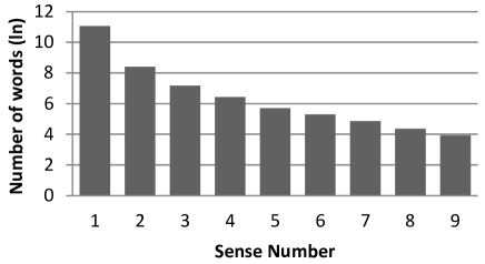
Figure 4: Distribution of sense numbers of words learned by D-GMSG.

Related Work

Recently, it has attracted lots of interests to learn word representation. Much previous works focus on learning word as a point vector in the embedded space. ? (?) applies the neural network to sentence modelling instead of using $n$-gram language models. Since the ? (?) model need expensive computational resource. Lots of works are trying to optimize it. ? (?) proposed the skip-gram model which is extremely efficient by removing the hidden layers of the neural networks, so that larger corpus could be used to train the word representation. By representing a word as a distributed vector, we gain a lot of interesting properties, such as similar words in syntactic or semantic roles are also close with each other in the embedded space in cosine distance or Euclidian distance. In addition, word embeddings also perform excellently in analogy tasks. For instance, $\mathbf{e}_{king}-\mathbf{e}_{queen}\approx\mathbf{e}_{man}-\mathbf{e}_{woman}$.

However, previous models mainly suffer from the polysemy problem. To address this problem, ? (?) represents words by constructing multiple sparse, high-dimensional vectors. ? (?) is an neural network based approach, which learns multiple dense, low-dimensional embeddings using global document context. ? (?) modeled the word polysemy from a probabilistic perspective and integrate it with the highly efficient continuous Skip-Gram model. ? (?) proposed Multi-Sense Skip-Gram (MSSG) to learn word sense embeddings with online word sense discrimination. These models perform word sense discrimination by clustering context of words. ? (?) discriminates word sense by introducing latent topic model to globally cluster the words into different topics. ? (?) further extended this work to model the complicated interactions of word embedding and its corresponding topic embedding by incorporating the tensor method.

Almost previous works are trying to use multiple points to represent the multiple senses of words. However, it cannot reflect the rich relations between words by simply representing words as points in the embedded space. ? (?) represented a word as a gaussian distribution. Gaussian mixture skip-gram (GMSG) model represents a word as a gaussian mixture distribution. Each sense of a word can be regarded as a gaussian component of the word. GMSG model gives different relations of words under different distance metrics, such as cosine distance, dot product, Euclidian distance KL divergence, etc.

Conclusions and Further Works

In this paper, we propose the Gaussian mixture skip-gram (GMSG) model to map a word as a density in the embedded space. A word is represented as a gaussian mixture distribution whose components can be regarded as the senses of the word. GMSG could reflect the rich relations of words when using different distance metrics. Since the number of word senses varies from word to word, we further propose the Dynamic GMSG (D-GMSG) model to adaptively increase the sense numbers of words during training.

Actually, a word can be regarded as any function including gaussian mixture distribution. In the further, we would like to investigate the properties of other functions for word representations and try to figure out the nature of the word semantic.

References

- [2003] Bengio, Y.; Ducharme, R.; Vincent, P.; and Janvin, C. 2003. A neural probabilistic language model. The Journal of Machine Learning Research 3:1137–1155.
- [2006] Bengio, Y.; Schwenk, H.; Senécal, J.-S.; Morin, F.; and Gauvain, J.-L. 2006. Neural probabilistic language models. In Innovations in Machine Learning. Springer. 137–186.
- [2008] Collobert, R., and Weston, J. 2008. A unified architecture for natural language processing: Deep neural networks with multitask learning. In Proceedings of ICML.
- [2011] Collobert, R.; Weston, J.; Bottou, L.; Karlen, M.; Kavukcuoglu, K.; and Kuksa, P. 2011. Natural language processing (almost) from scratch. The Journal of Machine Learning Research 12:2493–2537.
- [2011] Duchi, J.; Hazan, E.; and Singer, Y. 2011. Adaptive subgradient methods for online learning and stochastic optimization. The Journal of Machine Learning Research 12:2121–2159.
- [2001] Finkelstein, L.; Gabrilovich, E.; Matias, Y.; Rivlin, E.; Solan, Z.; Wolfman, G.; and Ruppin, E. 2001. Placing search in context: The concept revisited. In Proceedings of the 10th international conference on World Wide Web, 406–414. ACM.
- [2012] Huang, E.; Socher, R.; Manning, C.; and Ng, A. 2012. Improving word representations via global context and multiple word prototypes. In Proceedings of the 50th Annual Meeting of the Association for Computational Linguistics (Volume 1: Long Papers), 873–882. Jeju Island, Korea: Association for Computational Linguistics.
- [2002] Joachims, T. 2002. Optimizing search engines using clickthrough data. Proc. of SIGKDD.
- [2015] Liu, Y.; Liu, Z.; Chua, T.-S.; and Sun, M. 2015. Topical word embeddings. In AAAI.
- [2015] Liu, P.; Qiu, X.; and Huang, X. 2015. Learning context-sensitive word embeddings with neural tensor skip-gram model. In Proceedings of IJCAI.
- [2010] Mikolov, T.; Karafiát, M.; Burget, L.; Cernockỳ, J.; and Khudanpur, S. 2010. Recurrent neural network based language model. In INTERSPEECH.
- [2013a] Mikolov, T.; Chen, K.; Corrado, G.; and Dean, J. 2013a. Efficient estimation of word representations in vector space. arXiv preprint arXiv:1301.3781.
- [2013b] Mikolov, T.; Sutskever, I.; Chen, K.; Corrado, G. S.; and Dean, J. 2013b. Distributed representations of words and phrases and their compositionality. In NIPS, 3111–3119.
- [2013c] Mikolov, T.; Sutskever, I.; Chen, K.; Corrado, G. S.; and Dean, J. 2013c. Distributed representations of words and phrases and their compositionality. In Advances in Neural Information Processing Systems.
- [1991] Miller, G. A., and Charles, W. G. 1991. Contextual correlates of semantic similarity. Language and cognitive processes 6(1):1–28.
- [2007] Mnih, A., and Hinton, G. 2007. Three new graphical models for statistical language modelling. In Proceedings of ICML.
- [2005] Morin, F., and Bengio, Y. 2005. Hierarchical probabilistic neural network language model. In Proceedings of the international workshop on artificial intelligence and statistics, 246–252. Citeseer.
- [2014] Neelakantan, A.; Shankar, J.; Passos, A.; and McCallum, A. 2014. Efficient non-parametric estimation of multiple embeddings per word in vector space. In Proceedings of the Conference on Empirical Methods in Natural Language Processing (EMNLP).
- [2010] Reisinger, J., and Mooney, R. J. 2010. Multi-prototype vector-space models of word meaning. In Human Language Technologies: The 2010 Annual Conference of the North American Chapter of the Association for Computational Linguistics, 109–117. Association for Computational Linguistics.
- [2011] Socher, R.; Lin, C. C.; Manning, C.; and Ng, A. Y. 2011. Parsing natural scenes and natural language with recursive neural networks. In Proceedings of the 28th International Conference on Machine Learning (ICML-11), 129–136.
- [2013] Socher, R.; Bauer, J.; Manning, C. D.; and Ng, A. Y. 2013. Parsing with compositional vector grammars. In In Proceedings of the ACL conference. Citeseer.
- [2013] Szumlanski, S. R.; Gomez, F.; and Sims, V. K. 2013. A new set of norms for semantic relatedness measures. In ACL (2), 890–895.
- [2014] Tian, F.; Dai, H.; Bian, J.; Gao, B.; Zhang, R.; Chen, E.; and Liu, T.-Y. 2014. A probabilistic model for learning multi-prototype word embeddings. In Proceedings of COLING, 151–160.
- [2010] Turian, J.; Ratinov, L.; and Bengio, Y. 2010. Word representations: a simple and general method for semi-supervised learning. In Proceedings of the 48th annual meeting of the association for computational linguistics, 384–394. Association for Computational Linguistics.
- [2014] Vilnis, L., and McCallum, A. 2014. Word representations via gaussian embedding. arXiv preprint arXiv:1412.6623.
- [2011] Weston, J.; Bengio, S.; and Usunier, N. 2011. Wsabie: Scaling up to large vocabulary image annotation. In IJCAI, volume 11, 2764–2770.