Minimal $D=7$ Supergravity
and
the supersymmetry of Arnold-Beltrami Flux branes
P. Fré${}^{\;a,b,e}$, P.A. Grassi${}^{\;c,b}$, L. Ravera${}^{\;d,b}$, and M. Trigiante${}^{\;d,b}$
^aDipartimento di Fisica, Università di Torino
^bINFN – Sezione di Torino
via P. Giuria 1,  10125 Torino  Italy
e-mail:  fre@to.infn.it
^cDipartimento di Scienze e Innovazione Tecnologica,
Viale T. Michel 11, 15121 Alessandria, Italy Università del Piemonte Orientale,
e-mail:  pietro.grassi@uniupo.it
^dDISAT, Politecnico di Torino,
C.so Duca degli Abruzzi, 24, I-10129 Torino, Italy

e-mail: lucrezia.ravera@polito.it, mario.trigiante@polito.it

^eNational Research Nuclear University MEPhI
(Moscow Engineering Physics Institute),
Kashirskoye shosse 31, 115409 Moscow, Russia

In this paper we study some properties of the newly found Arnold-Beltrami flux-brane solutions to the minimal $D=7$ supergravity. To this end we first single out the appropriate Free Differential Algebra containing both a gauge $3$-form $\mathbf{B}^{[3]}$ and a gauge $2$-form $\mathbf{B}^{[2]}$: then we present the complete rheonomic parametrization of all the generalized curvatures. This allows us to identify two-brane configurations with Arnold-Beltrami fluxes in the transverse space with exact solutions of supergravity and to analyze the Killing spinor equation in their background. We find that there is no preserved supersymmetry if there are no additional translational Killing vectors. Guided by this principle we explicitly construct Arnold-Beltrami flux two-branes that preserve $0$, ${\textstyle\frac{1}{8}}$ and ${\textstyle\frac{1}{4}}$ of the original supersymmetry. Two-branes without fluxes are instead $\mathrm{BPS}$ states and preserve ${\textstyle\frac{1}{2}}$ supersymmetry. For each two-brane solution we carefully study its discrete symmetry that is always given by some appropriate crystallographic group $\Gamma$. Such symmetry groups $\Gamma$ are transmitted to the $D=3$ gauge theories on the brane world–volume that occur in the gauge/gravity correspondence. Furthermore we illustrate the intriguing relation between gauge fluxes in two-brane solutions and hyperinstantons in $D=4$ topological sigma-models.

1 Introduction

Minimal Supergravity in $D=7$ contains 16 supercharges and it is usually named $\mathcal{N}=2$ since the 16 supercharges are arranged into a pair of pseudo-Majorana spinors.

The Poincaré (ungauged) version of the theory has been constructed independently by Townsend and van Nieuwenhuizen in [1] and by Salam and Sezgin in [2] in two different formulations that use respectively a three-form gauge field $\mathbf{B}^{[3]}_{\mu\nu\rho}$ and a two-form gauge field $\mathbf{B}^{[2]}_{\mu\nu}$, in addition to the graviton $g_{\mu\nu}$, the gravitino $\Psi_{A|\mu}^{\alpha}$ ($\alpha=1,\dots,8$, $\mu\,=\,0,1,\dots,6$, $A\,=\,1,2$), the dilatino $\chi_{A}^{\alpha}$, three gauge fields $\mathcal{A}^{\Lambda}_{\mu}$ ($\Lambda\,=\,1,2,3$) and the dilaton $\phi$, that are common to both formulations. From the on-shell point of view the number of degrees of freedom described by either $\mathbf{B}^{[3]}_{\mu\nu\rho}$ or $\mathbf{B}^{[2]}_{\mu\nu}$ is the same and the two types of gauge fields are electric-magnetic dual to each other.

The gauging of the theory was also independently considered both in [1] and in [2]. The coupling of minimal $D=7$ supergravity to $n$ vector multiplets was constructed by Bergshoeff et al in [3] on the basis of the two-form formulation and shown to be based on the use of the coset manifold:

$$\mathcal{M}_{3n+1}\,=\,\mathrm{SO(1,1)}\,\times\,\frac{\mathrm{SO(3,n)}}{\mathrm{SO(3)\times SO(n)}}$$ (1.1)

as scalar manifold that encodes the spin zero degrees of freedom of the theory.

In all the quoted references the construction was done using the Noether coupling procedure, up to four-fermion terms in the Lagrangian and up to two-fermion and three-fermion terms in the transformation rules. Correspondingly the on-shell closure of the supersymmetry algebra was also checked only up to such terms.

There is a renewed interest in this supergravity theory in relation with the classification of Arnold-Beltrami fields [4] recently obtained by one of us, in a different collaboration, in [10]. These fields, originally introduced by Beltrami as solutions of the first order equation that bears his name [4], were shown to have high relevance in mathematical hydrodynamics by Arnold who proved a famous theorem according to which the only flows capable of admitting chaotic streamlines are the Beltrami flows [5, 6, 8]. This theorem originated a vast literature on the so named ABC-flows that correspond to the simplest solutions of Beltrami equation [7, 9]. The Beltrami vector fields live on three-dimensional tori and in mathematical hydrodynamics are interpreted as velocity fields of some fluid. They can also be used as compactification fluxes in the transverse space to the world volume of $2$-brane solutions of $D=7$ supergravity theory. This new interpretation of Beltrami fields, jocosely described by the authors as a Sentimental Journey from Hydrodynamics to Supergravity, was proposed in [11]. In this way the rich discrete symmetries of Arnold-Beltrami fields that are now turned from flows into fluxes can be transmitted to the three dimensional gauge theories living on the world volume of the two-brane. Another intriguing relation of this type of $\mathrm{3D}$-vector fields with the tri-holomorphic hyperinstantons, namely with the instanton configurations of four-dimensional sigma-models that are singled out by the topological twist, was recently pointed in [12].

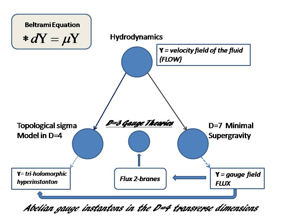
Figure 1:

The intriguing set of multi-sided relations implied by different interpretations of Beltrami vector fields is graphically summarized in fig.1 which provides a sort of conceptual map for the present paper.

In [11] the explicit construction of $2$-brane solutions with Arnold-Beltrami fluxes was performed but their embedding in $d=7$ supergravity was not discussed and what is the most relevant issue, namely the residual supersymmetry that they might preserve, was not explored. This is the main goal of the present paper.

With this motivation, we have first reconsidered the construction of minimal $D=7$ supergravity in the approach based on Free Differential Algebras and rheonomy (for reviews see [14] and also the second volume of [15]). The goal is that of clarifying the algebraic structure underlying the theory, thus providing a solid basis for the analysis of the $2$-branes mentioned above. In this systematic revisitation of $D=7$ supergravity we have found several subtleties whose clarification was in our opinion extremely important, in particular in relation with the double formulation in terms of $\mathbf{B}^{[3]}_{\mu\nu\rho}$ and $\mathbf{B}^{[2]}_{\mu\nu}$ which obviously plays a primary role for brane solutions.

In this paper we present the complete rheonomic solution of Bianchi identities which, as it is well known, implicitly implies the fermionic and bosonic field equations of all the fields. The request that the rheonomic parameterizations of the $2$-form curvature $\mathfrak{G}^{[3]}$ and of the 3-form curvature $\mathfrak{G}^{[4]}$ should be compatible completely fixes all the coefficients in the rheonomic parameterizations and therefore determines all supersymmetry transformation rules including higher order terms in the fermion fields. As we show, upon suitable rescalings, these transformation rules fully coincide with those derived (up to linear order in the fermions) by the authors of [1, 3]. This is a very significant consistency test that goes hand in hand with another important test already obtained in [11]. There it was shown that Beltrami flux $2$ brane solutions of a bosonic theory with the same content as $D=7$ supergravity can exist if and only if the ratios between the coefficients in the action are exactly the same as those determined by the authors of [1]. This leads to an exact prediction on the bosonic subset of the coefficients appearing in the geometric lagrangian of $D=7$ supergravity, whose explicit form is still under construction. We plan to present it in a forthcoming paper.

The information mentioned above is sufficient to embed the Arnold-Beltrami flux-branes into $D=7$ supergravity and to write down the precise form of the Killing spinor equation in general terms and to polarize on this type of backgrounds.

The second main result of this paper is the analysis of the supersymmetry preserved by $2$-branes and flux $2$-branes. Without fluxes the $2$-branes preserve ${\textstyle\frac{1}{2}}$ of the original supersymmetry and they always admit eight Killing spinors. With Arnold-Beltrami fluxes supersymmetry is usually completely broken, unless the solution, besides discrete symmetries has also extra translational Killing vectors. With two translational Killing vectors one can preserve ${\textstyle\frac{1}{4}}$ of the original supersymmetry, corresponding to the presence of four Killing spinors. With one translational Killing vector one can preserve ${\textstyle\frac{1}{8}}$ of the original supersymmetry, corresponding to the presence of two Killing spinors. The presence of the translational Killing vectors is a necessary, yet not sufficient condition. Accurate choices of the fluxes have to be made which lead to certain precise discrete symmetries illustrated in our worked out examples.

Our paper is organized as follows

a)

In section 2 we review the construction, introduced in [11] of two-branes in seven dimensions with Arnold Beltrami Fluxes in the transverse space.

b)

In section 3 we discuss the algebraic basis of $D=7$ supergravity. In particular, utilizing crucial Fierz identities we derive the underlying Free Differential Algebra and we analyze its properties.

c)

In section 4 we address the geometric construction of $D=7$ supergravity introducing the rheonomic parameterizations of the curvatures and the general form of the action. The actual determination of the coefficients is provided in Appendix A.

d)

In section 5 we discuss the explicit embedding of the flux brane solutions into supergravity. This is a necessary essential intermediate step in order to be able to discuss the residual supersymmetry.

e)

In section 6 we write the Killing spinor equation and investigate its general properties. There we present the logic of a computerized algorithm devised to investigate the presence or absence of Killing spinors.

f)

In section 7 we present three explicit cases of flux $2$-brane solutions with zero, ${\textstyle\frac{1}{4}}$ and ${\textstyle\frac{1}{2}}$ preserved supersymmetry, respectively. We carefully discuss the discrete symmetries of these solutions.

g)

In section 8 we briefly discuss the uplifting of Arnold Beltrami flux 2-branes to $D=11$ supergravity.

e)

Section 9 contains our conclusions.

2 D=7 two-branes with Arnold Beltrami Fluxes in the transverse directions

In this section we review the construction of [11] based on the general form of $p$-brane actions which is described in many places in the literature (in particular we refer the reader to chapter 7, Volume Two of [15] and to all the papers there cited) and we focus on the the case $p\,=\,2$ in $D=7$. The concern of [11] was the elementary $2$-brane solution in $D=7$. It was shown in [11] that this latter exists for all values of the exponential coupling parameter $a$ defined below. Each value of $a$ corresponds to a different value of the dimensional reduction invariant parameter $\Delta$ also defined below. Obviously $D=7$ supergravity corresponds to a unique value of $\Delta$ which, as we recall in section B.1, is the magic $\Delta\,=\,4$ for which the solution becomes particularly simple and elegant and typically preserves one half of the supersymmetries.

Subsequently, in [11], on the background of the $2$-brane solution it was considered the inclusion of fluxes of an additional triplet of vector fields, in this way mimicking the bosonic field content of $D=7$ supergravity. In presence of a topological interaction term between the triplet of gauge fields and the $3$-form which defines the $2$-brane, it was shown that the fluxes can be introduced into the framework of an exact solution if they are Arnold Beltrami vector fields satisfying Beltrami equation. The only conditions for the existence of such a solution is $\Delta\,=\,4$ plus a precise relation between the coefficients of the kinetic terms in the lagrangian and the coefficient of the topological interaction term. Clearly this relation is precisely satisfied by the coefficients of minimal $D=7$ supergravity as we show in the present paper.

2.1 The general form of a $2$-brane action in $D=7$

In the mostly minus metric that we utilize, the correct form of the action in $D=7$ admitting an electric $2$-brane solution is the following one:

$$\mathcal{A}_{2brane} = \int\,d^{7}x\,\mathcal{L}_{2brane}$$

$$\mathcal{L}_{2brane} = \mbox{det}V\,\left(-R[g]\,-\,{\textstyle\frac{1}{4}}\,\partial^{\mu}\varphi\,\partial_{\mu}\varphi\,+\,{\textstyle\frac{1}{96}}\,e^{-a\,\varphi}\,\mathbf{F}_{\lambda\mu\nu\rho}\,\mathbf{F}^{\lambda\mu\nu\rho}\right)$$ (2.1)

where $a$ is a free parameter, $\varphi$ denotes the dilaton field with a canonically normalized kinetic term and :

$$\mathbf{F}_{\lambda\mu\nu\rho}\,\equiv\,\partial_{[\lambda}\,\mathbf{A}_{\mu\nu\rho]}$$ (2.2)

is the field-strength of the three-form $\mathbf{A}^{[3]}$ which couples to the world volume of the two-brane.

The field equations following from (2.1) can be put into the following convenient form:

$$\Box_{cov}\,\varphi = \frac{a}{48}e^{-a\varphi}\,\mathbf{F}_{\lambda\mu\nu\rho}\,\mathbf{F}^{\lambda\mu\nu\rho}$$ (2.3)

$$\mathrm{d}\star\left[e^{-a\varphi}\,\star\mathbf{F}^{[4]}\right] = 0$$ (2.4)

$$\mbox{Ric}_{\mu\nu} = \frac{1}{4}\partial_{\mu}\varphi\,\partial_{\nu}\varphi\,+\,S_{\mu\nu}$$ (2.5)

$$S_{\mu\nu} = -\,\frac{1}{24}e^{-a\varphi}\left(\mathbf{F}_{\mu...}\,\mathbf{F}_{\nu}^{\phantom{\nu}...}\,-\,{\textstyle\frac{3}{20}}\,g_{\mu\nu}\,\mathbf{F}_{....}\,\mathbf{F}^{....}\right)$$ (2.6)

and they admit the following exact electric $2$-brane solution:

$$ds^{2} = H(y)^{-\frac{8}{5\Delta}}\,d\xi^{\mu}\otimes d\xi^{\nu}\,-\,H(y)^{\frac{12}{5\Delta}}\,dy^{I}\otimes dy^{J}\,\delta_{IJ}$$

$$\varphi = -\frac{2a}{\Delta}\,\log\,H(y)$$

$$\mathbf{F}_{[4]} = 4\,\mathrm{d}\left[H(y)^{-1}\,\mathrm{d}\xi^{\mu}\wedge\mathrm{d}\xi^{\nu}\wedge\mathrm{d}\xi^{\rho}\,\epsilon_{\mu\nu\rho}\right]$$ (2.7)

where the seven coordinates have been separated into two sets $\xi^{\mu}$ ($\mu=0,1,2$) spanning the $2$-brane world volume and $y^{I}$ ($I=3,4,5,6$) spanning the transverse space to the brane. In the above solution $H(y)$ is any harmonic function living on the $4$-dimensional transverse space to the brane whose metric is assumed to be flat:

$$\Box_{\mathbb{R}^{4}}\,H(y)\,\equiv\,\sum_{I=1}^{4}\frac{\partial^{2}}{\partial(y^{I})^{2}}H(y)\,=\,0$$ (2.8)

and the parameters $a$ and $\Delta$ are related by the celebrated formula:

$$\Delta\,=\,a^{2}\,+\,2\frac{d\,\widetilde{d}}{D-2}\,=\,a^{2}\,+\,\frac{12}{5}$$ (2.9)

which follows from $d=3,\quad\widetilde{d}\,=\,2$ and $D=7$. Physically $d$ is the dimension of the electric $2$-brane world volume, while $\widetilde{d}$ is the dimension of the world-sheet spanned by the magnetic string which is dual to the $2$-brane.

In section B.1 we will discuss the relation of the brane action (2.1) with the bosonic action of Minimal ungauged $D=7$ supergravity and show that the specific coefficients of the kinetic terms appearing in this latter determine the value of $\Delta$. Indeed the supersymmetry of the action imposes $\Delta\,=\,4$. In a later section we discuss the Killing spinors admitted by the solution (2.7).

2.2 The two-brane with Arnold Beltrami Fluxes

As a next step, in [11] the two-brane action (2.1) was generalized introducing also a triplet of one-form fields $\mathbf{A}^{\Lambda}$, ($\Lambda\,=\,1,2,3$) whose field strengths are denoted $\mathbf{F}^{\Lambda}\,\equiv\,\mathrm{d}\mathbf{A}^{\Lambda}$. In this way we mimic the field-content of Minimal $D=7$ supergravity. Explicitly one has the new bosonic action:

$$\mathcal{A}^{flux}_{2brane} = \int\,d^{7}x\,\mathcal{L}^{flux}_{2brane}$$

$$\mathcal{L}^{flux}_{2brane} = \mbox{det}V\,\left(-R[g]\,-\,{\textstyle\frac{1}{4}}\,\partial^{\mu}\varphi\,\partial_{\mu}\varphi\,+\,{\textstyle\frac{1}{96}}\,e^{-a\,\varphi}\,\mathbf{F}_{\lambda\mu\nu\rho}\,\mathbf{F}^{\lambda\mu\nu\rho}\right.$$ (2.10)

$$\left.+\,{\textstyle\frac{\omega}{8}}\,e^{{\textstyle\frac{a}{2}}\varphi}\,\mathbf{F}^{\Lambda}_{\lambda\mu\ }\,\mathbf{F}^{\Lambda|\lambda\mu}\right)\,-\,\kappa\,\,\mathbf{F}_{\lambda_{1}\dots\lambda_{4}}\,\mathbf{F}^{\Lambda}_{\lambda_{5}\lambda_{6}}\,\mathbf{A}^{\Lambda}_{\lambda_{7}}\,\epsilon^{\lambda_{1}\dots\lambda_{7}}$$

where two new real parameters $\omega$ and $\kappa$ do appear. Crucial for the consistent insertion of fluxes is the topological interaction term with coefficient $\kappa$.

The modified field equations associated with the new action (2.10) can be written in the following way:

$$\Box_{cov}\,\varphi = \frac{a}{48}e^{-a\varphi}\,\mathbf{F}_{\lambda\mu\nu\rho}\,\mathbf{F}^{\lambda\mu\nu\rho}\,-\,\omega\frac{a}{8}e^{a\varphi}\,\mathbf{F}^{\Lambda}_{\lambda\mu}\,\mathbf{F}^{\Lambda|\lambda\mu}$$ (2.11)

$$\mathrm{d}\left[e^{-a\varphi}\,\star\mathbf{F}^{[4]}\right] = 1152\,\kappa\,\,\mathbf{F}^{\Lambda}\,\wedge\,\mathbf{F}^{\Lambda}$$ (2.12)

$$\mathrm{d}\left[e^{{\textstyle\frac{a}{2}}\varphi}\,\star\mathbf{F}^{\Lambda}\right] = 8\,\frac{\kappa}{\omega}\,\,\mathbf{F}^{[4]}\,\wedge\,\mathbf{F}^{\Lambda}$$ (2.13)

$$\mbox{Ric}_{\mu\nu} = \frac{1}{4}\partial_{\mu}\varphi\,\partial_{\nu}\varphi\,+\,S^{[4]}_{\mu\nu}\,+\,S^{[2]}_{\mu\nu}$$ (2.14)

$$S^{[4]}_{\mu\nu} = -\,\frac{1}{24}e^{-a\varphi}\left(\mathbf{F}_{\mu...}\,\mathbf{F}_{\nu}^{\phantom{\nu}...}\,-\,{\textstyle\frac{3}{20}}\,g_{\mu\nu}\,\mathbf{F}_{....}\,\mathbf{F}^{....}\right)$$ (2.15)

$$S^{[2]}_{\mu\nu} = -\,\omega\,\frac{1}{4}e^{{\textstyle\frac{a}{2}}\varphi}\left(\mathbf{F}^{\Lambda}_{\mu.}\,\mathbf{F}_{\nu}^{\Lambda|\phantom{\nu}.}\,-\,{\textstyle\frac{1}{10}}\,g_{\mu\nu}\,\mathbf{F}^{\Lambda}_{..}\,\mathbf{F}^{\Lambda|..}\right)$$ (2.16)

In [11] the above equations were solved with the same ansatz as in the previous case for the metric, the dilaton and the $4$-form, introducing also a non trivial $\mathbf{F}^{\Lambda}$ in the transverse space spanned by the coordinates $y$. Explicitly, the ansatz considered in [11] is the following one.

$$ds^{2} = H(y)^{-\frac{8}{5\Delta}}\,d\xi^{\mu}\otimes d\xi^{\nu}\,-\,H(y)^{\frac{12}{5\Delta}}\,dy^{I}\otimes dy^{J}\,\delta_{IJ}$$

$$\varphi = -\frac{2a}{\Delta}\,\log\,H(y)$$

$$\mathbf{F}_{[4]} = 4\,\mathrm{d}\left[H(y)^{-1}\,\mathrm{d}\xi^{\mu}\wedge\mathrm{d}\xi^{\nu}\wedge\mathrm{d}\xi^{\rho}\,\epsilon_{\mu\nu\rho}\right]$$

$$\mathbf{F}^{\Lambda} = \mathrm{d}\left[\mathbf{W}^{\Lambda}_{I}(y)\,dy^{I}\right]$$ (2.17)

2.2.1 Arnold Beltrami vector fields on the torus $\mathrm{T}^{3}$ as fluxes

In order to solve the above equations a change of topology was put forward in [11]. In the brane solutions without fluxes the transverse space to the brane volume was chosen flat and non compact, namely $\mathbb{R}^{4}$. To introduce the fluxes one mantains it flat but one compactifies three of its dimensions by identifying them with those of a three-torus $\mathrm{T}^{3}$. In other words one performs the replacement:

$$\mathbb{R}^{4}\,\rightarrow\,\mathbb{R}_{+}\otimes\mathrm{T}^{3}$$ (2.18)

Secondly, on the abstract $\mathrm{T}^{3}$-torus one utilizes the flat metric consistent with octahedral symmetry, namely according to the setup of [10] one identifies:

$$\mathrm{T}^{3}\,\simeq\,\frac{\mathbb{R}^{3}}{\Lambda_{cubic}}$$ (2.19)

where $\Lambda_{cubic}$ denotes the cubic lattice, i.d. the abelian group of discrete translations of the euclidian three-coordinates $\left\{X,Y,Z\right\}$, defined below:

$$\Lambda_{cubic}\,\ni\,\gamma_{n_{1},n_{2},n_{3}}\quad:\quad\left\{X,Y,Z\right\}\,\rightarrow\,\left\{X+n_{1},Y+n_{2},Z+n_{3}\right\}\quad;\quad n_{1,2,3}\,\in\,\mathbb{Z}$$ (2.20)

Functions on $\mathrm{T}^{3}$ are periodic functions of $X,Y,Z$, with respect to the translations (2.20).

According to (2.18) one splits the four coordinates $y^{I}$ as follows:

$$y^{I}\,=\,\left\{\underbrace{U}_{\in\,\mathbb{R}}\,,\,\underbrace{X,Y,Z}_{\equiv\,\mathbf{X}\,\in\,\mathrm{T}^{3}}\right\}$$ (2.21)

In [10], one of us, in a different collaboration, has classified and constructed all the solutions of Beltrami equation:

$$\star\,\mathrm{d}\mathbf{Y}^{[1]}\,=\,\mu\,\mathbf{Y}^{[1]}$$ (2.22)

for one-forms $\mathbf{Y}^{[1]}$ defined over the three-torus (2.19) outlining the strategy to construct the same solutions also in the case of other crystallographic lattices like, for instance, the hexagonal one. These solutions are organized in orbits with respect to the cubic lattice point group, namely the 24-elements octahedral group $\mathcal{O}_{24}$ and their parameter space is decomposed into irreducible representations of appropriate subgroups of a universal classifying group with $1536$ elements [10]. Using such one-forms $\mathbf{Y}^{[1]}$ as building blocks for the brane fluxes appeared very appealing in [11] since it introduces the corresponding discrete symmetries into the brane solution.

Explicitly the last of the ansätze (2.17) was specialized in the following way:

$$\mathbf{F}^{\Lambda} = \lambda\,\mathrm{d}\,\left[e^{2\pi\mu U}\,\mathbf{W}^{\Lambda}\left(\mathbf{X}\right)\right]$$ (2.23)

$$\mathbf{W}^{\Lambda}\left(\mathbf{X}\right) = \mathcal{E}^{\Lambda}_{\phantom{\Lambda}A}\,\mathbf{Y}^{A}\left(\mathbf{X}\right)$$ (2.24)

where $\mathbf{Y}^{A}\left(\mathbf{X}\right)$ denotes a basis of solutions of Beltrami equation (2.22) pertaining to eigenvalue $\mu$ and the embedding matrix $\mathcal{E}^{\Lambda}_{\phantom{\Lambda}A}$ is a constant matrix which constructs three linear independent combinations of such fields. Furthermore $\lambda$ is some numerical parameter.

It was shown in [11] that all field equations (2.11-2.16) are solved if the following conditions are verified

$$\Delta = 4\,\Leftrightarrow\,a\,=\,2\,\sqrt{\frac{2}{5}}$$

$$\kappa = \frac{\omega}{384}$$

$$\Box_{\mathbb{R}_{+}\times\mathrm{T}^{3}}\,H(U,\mathbf{X}) = -\,\frac{\lambda^{2}}{24}\,\exp\left[2\,\pi\,\mu\,U\right]\,\mu^{2}\,J(\mathbf{X})$$

$$J(\mathbf{X}) \equiv \sum_{\Lambda=1}^{3}\,\sum_{i=1}^{3}\,\mathbf{W}^{\Lambda}(\mathbf{X})_{i}\mathbf{W}^{\Lambda}(\mathbf{X})_{i}$$ (2.25)

The first two conditions of (2.25) are a specification of the parameters in the brane lagrangian. It was already noted in [11] that such a specification corresponds to selecting a bosonic lagrangian that, up to field redefinitions, is equivalent to the bosonic lagrangian of minimal $D=7$ supergravity. The third equation is the only differential condition that solves the entire system of field equations. The function $H(y)$ appearing in the metric, in the dilaton and in the three-form $\mathbf{B}^{[3]}$ needs to satisfy a inhomogeneous Laplace equation whose source $J(\mathbf{X})$ is entirely determined by the Beltrami vector fields according to the formula displayed in the last of eq.s (2.25).

2.3 Relation of the Arnold-Beltrami Fluxes with Hyperinstantons

In the recent paper [12] the relation between Beltrami equation (2.22) and the defining equation of tri-holomorphicity was explored. It was shown in the past in [13] that a suitable definition of what we can name a tri-holomorphic map from a flat HyperKähler four–dimensional manifold $\mathcal{HK}_{4}$ to any HyperKähler manifold $\mathcal{HK}_{4n}$:

$$q\,:\,\mathcal{HK}_{4}\,\rightarrow\,\mathcal{HK}_{4n}$$ (2.26)

naturally emerges from the topological twist of an $\mathcal{N}=2$ supersymmetric sigma model in $D=4$. The following first order differential equation:

$$q^{\star}-\sum_{x=1}^{3}\,J_{x}\circ q^{\star}\circ j_{x}=0,$$ (2.27)

where $J^{x}$ denote the three complex structures of the target manifold $\mathcal{HK}_{4n}$ and $j^{x}$ those of the base manifold is obtained as the BRST-variation of the antighost produced by the twist. Henceforth eq.(2.27) defines in a unique algebraic way the instantonic maps on which the functional integral should be localized in the topological version of the sigma-model. For this reason the maps satisfying eq.(2.27) were dubbed hyperinstantons in [13] and it was also observed that they are tri-holomorphic since eq.(2.27) can be interpreted as the statement that they are holomorphic with respect to the average of the three complex structures. In [12] the base manifold was chosen to be $\mathbb{R}_{+}\times\mathrm{T^{3}}$ while the target manifold was simply chosen to be $\mathbb{R}^{4}$. In this way the equation of tri-holomorphicity was applied to maps:

$$q\,:\,\mathbb{R}_{+}\times\mathrm{T^{3}}\,\rightarrow\,\mathbb{R}^{4}$$ (2.28)

It was shown in [12] that, under very mild assumptions, the general solution of equation (2.27) is as follows. Let $G(\mathbf{X})$ be a generic function on the $\mathrm{T^{3}}$ torus , let $\mathbf{Y}(\mathbf{X})$ be a solution of Beltrami equation (2.22) corresponding to eigenvalue $\mu$ and define:

$$\Phi\left(\mathrm{U},\mathbf{X}\right) = e^{-2\,\mu\,\mathrm{U}}\,G\left(\mathbf{X}\right)$$

$$\mathbf{A}\left(\mathrm{U},\mathbf{X}\right) = e^{-\,2\,\mu\,\mathrm{U}}\,\mathbf{Y}\left(\mathbf{X}\right)$$ (2.29)

where $U$ is the positive real variable spanning $\mathbb{R}_{+}$. Then the image of the point $\{U,\mathbf{X}\}\in\mathbb{R}_{+}\times\mathrm{T^{3}}$ with respect to a map $q$ that satisfies the tri-holomorphic constraint (2.27) is given by $\{q_{0},\mathbf{q}\}\in\mathbb{R}^{4}$, where:

$$q_{0}\left(\mathrm{U},\mathbf{X}\right) = \,-\,\partial_{\mathrm{U}}\,\Phi\left(\mathrm{U},\mathbf{X}\right)$$

$$\mathbf{q}\left(\mathrm{U},\mathbf{X}\right) = \,\nabla\,\Phi\left(\mathrm{U},\mathbf{X}\right)\,+\,\mathbf{A}\left(\mathrm{U},\mathbf{X}\right)$$ (2.30)

the operator $\nabla$ representing the derivatives with respect to the torus coordinates.

Next, if we interpret the four components $\{q_{0},\mathbf{q}\}$ as the components of a gauge $1$-form in $\mathbb{R}_{-}\times\mathrm{T^{3}}$ (where $\mathrm{U}\to-U$), namely if we set:

$$\mathcal{A}\,=\,q_{0}\mathrm{d}U\,+\,\mathbf{q}\cdot\mathrm{d}\mathbf{X}$$ (2.31)

we obtain:

$$\mathcal{A}\,=\,\mathrm{d}\Phi\left(U,\mathbf{X}\right)\,+\,e^{-2\,\mu\,\mathrm{U}}\,\mathbf{Y}$$ (2.32)

We recall also that this gauge connection satisfies a suitable gauge fixing (see [12] for a complete discussion). It appears clearly from eq. (2.32) that the function $\Phi\left(U,\mathbf{X}\right)$ is just an irrelevant gauge transformation which has no influence on the gauge field strengths appearing in supergravity. Apart from it the gauge fields entering the brane solutions as fluxes are just hyperinstantons in the transverse directions to the brane, namely on $\mathbb{R}_{-}\times\mathrm{T^{3}}$. The restriction to $\mathbb{R}_{-}\Leftrightarrow\mathbb{R}_{+}$ on the sigma-model side of this correspondence is greatly illuminated by it. Indeed on the supergravity side $U$ has to be negative in order to keep the metric real. Choosing the parameter $\lambda$ appropriately we can arrange that $U=0$, which is a boundary in the sigma model, corresponds to a metric singularity in supergravity. This singularity is the brane itself, since $U$ is nothing else but the distance from the brane.

3 The algebraic basis of $D=7$ supergravity

Motivated by $2$-branes with Arnold-Beltrami fluxes that we have summarized in the previous section, we turn to the reconstruction of $D=7$ supergravity in a systematic algebro-geometric approach. Our final aim is to embed the considered $2$-branes in supergavity and to investigate their supersymmetries.

As announced in the introduction, in the present section we clarify the algebraic basis of minimal $D=7$ supergravity in terms of Free Differential Algebras, preparing the stage for its ex novo reconstruction in the rheonomic approach.

3.1 Pseudo Majorana spinors in $D=7$

The main property of the Clifford algebra in $D=7$ with Minkowski signature (see eq.(C.1)) is that there is only one type of conjugation matrix, namely $\mathcal{C}_{-}$ (see [14],[15]) and that this latter is symmetric:

$$\mathcal{C}_{-}\,\Gamma_{a}\,\mathcal{C}_{-}^{-1}\,=\,-\,\Gamma_{a}^{T}\quad;\quad\mathcal{C}_{-}\,=\,\mathcal{C}_{-}^{T}\quad;\quad\mathcal{C}_{-}^{2}\,=\,\mathbf{1}_{8\times 8}$$ (3.1)

This being the case one can always choose a basis where $\mathcal{C}_{-}$ is just the identity matrix in eight-dimensions and the gamma–matrices are all antisymmetric as described in appendix C.1 Hence there are no Majorana spinors but, just as in $d=5$, we can introduce doublets of pseudo-Majorana gravitino one-forms. Minimal $D=7$ supergravity corresponds to the case where we have just one such doublet that we name $\Psi_{A}$ ($A\,=\,1,2$):

$$\Psi_{A}^{c}\,\equiv\,(\overline{\Psi}^{A})^{T}\,=\,-\,\Gamma_{0}\Psi_{A}^{\star}\,=\,\epsilon^{AB}\,\Psi_{A}$$ (3.2)

An explicit solution of the pseudo-Majorana constraint in the gamma matrix basis described in appendix C.1 is shown below:

$$\Psi_{1}\,=\,\left(\begin{array}[]{l}\alpha_{1}+i\beta_{1}\\ \alpha_{2}+i\beta_{2}\\ \alpha_{3}+i\beta_{3}\\ \alpha_{4}+i\beta_{4}\\ \alpha_{5}+i\beta_{5}\\ \alpha_{6}+i\beta_{6}\\ \alpha_{7}+i\beta_{7}\\ \alpha_{8}+i\beta_{8}\end{array}\right)\quad;\quad\Psi_{2}\,=\,\left(\begin{array}[]{l}-i\alpha_{7}-\beta_{7}\\ -i\alpha_{3}-\beta_{3}\\ i\alpha_{2}+\beta_{2}\\ -i\alpha_{8}-\beta_{8}\\ i\alpha_{6}+\beta_{6}\\ -i\alpha_{5}-\beta_{5}\\ i\alpha_{1}+\beta_{1}\\ i\alpha_{4}+\beta_{4}\end{array}\right)$$ (3.3)

where $\alpha_{1,\dots,8}$ and $\beta_{1,\dots,8}$ are real components. This explicitly shows that minimal $D=7$ supergravity is based on a superalgebra with $16$ supercharges, just one half of the maximum $32$.

When we discuss Killing spinors for the $2$-brane solutions we utilize another gamma matrix basis well adapted to the split of $7$-dimensions in $3+4$. Such a basis is described in appendix C.2. The explicit form of a pair of pseudo-Majorana spinors in this basis is provided here below:

$$\begin{array}[]{ccccccc}\epsilon_{1}&=&\left(\begin{array}[]{c}\xi_{1}-i\xi_{2}\\ \xi_{3}+i\xi_{4}\\ \theta_{1}-i\theta_{6}\\ \theta_{2}+i\theta_{5}\\ \xi_{5}-i\xi_{6}\\ \xi_{7}+i\xi_{8}\\ \theta_{3}-i\theta_{8}\\ \theta_{4}+i\theta_{7}\\ \end{array}\right)&;&\epsilon_{2}&=&\left(\begin{array}[]{c}\xi_{4}+i\xi_{3}\\ \xi_{2}-i\xi_{1}\\ \theta_{5}+i\theta_{2}\\ \theta_{6}-i\theta_{1}\\ \xi_{8}+i\xi_{7}\\ \xi_{6}-i\xi_{5}\\ \theta_{7}+i\theta_{4}\\ \theta_{8}-i\theta_{3}\\ \end{array}\right)\end{array}$$ (3.4)

where $\xi_{1},\dots,\xi_{8}$ and $\theta_{1},\dots,\theta_{8}$ are two octets of real anticommuting parameters. The particular form of this parameterization is already adapted to the projection that will be enforced by the spin one-half fermion transformation rules in the Killing spinor equation. This projection will simply delete the eight parameters $\theta$.

3.2 Fierz identities

As usual, the core of any supergravity construction is provided by the $4$-$\Psi$ and $3$-$\Psi$ Fierz identities. Indeed from the $4$-$\Psi$ Fierz identities one obtains the available Chevalley cocycles that give rise to the Free-Differential Algebra extension of the super Poincaré algebra. This latter encodes the $p$-form gauge fields that complete the gravitational multiplet. On the other hand $3$-$\Psi$ Fierz are crucial in the construction of a rheonomic parameterization of the curvature which solves Bianchi identities.

The first step in this analysis is provided by counting the $2$-$\Psi$ independent components and arranging them into a complete set of bosonic-currents. In this case, since we have $16$-supercharges, the number of independent components of the symmetric wedge product is

$$\mbox{\# of components of}\,\,\Psi^{\alpha}_{A}\,\wedge\,\Psi^{\beta}_{B}\,=\,{\textstyle\frac{1}{2}}\,16\times 17\,=\,136$$ (3.5)

Introducing the three Pauli matrices $\sigma^{\Lambda|A}_{\phantom{\Lambda|A}B}$ ($\Lambda\,=\,1,2,3$, $A,B\,=\,1,2$) according to the conventions of appendix C.1.1 we can distribute the 136 components in the following exhaustive set of fermionic currents:

name		current	# of components
$\mathbf{J}^{a}$	=	$\overline{\Psi}^{A}\,\wedge\,\Gamma^{a}\,\Psi_{A}$	7
$\mathbf{J}^{ab}$	=	${\rm i}\,\overline{\Psi}^{A}\,\wedge\,\Gamma^{ab}\,\Psi_{A}$	21
$\mathbf{J}^{\Lambda}$	=	${\rm i}\,\sigma^{\Lambda|B}_{\phantom{\Lambda|B}A}\,\overline{\Psi}^{A}\,\wedge\,\Psi_{B}$	3
$\mathbf{J}^{\Lambda}_{pqr}$	=	i  $\sigma^{\Lambda|B}_{\phantom{\Lambda|B}A}\,\overline{\Psi}^{A}\,\wedge\,\Gamma_{pqr}\Psi_{B}$	105
			136

The factors ${\rm i}$ have been placed in the above formulae in such a way as to make the corresponding fermion currents real. There are two fundamental $4$-$\Psi$ Fierz identities that might be deduced by means of group theory, counting the number of singlet representations that appear in the symmetric product of $4$-$\Psi$ but which we have simply verified with a computer programme by direct evaluation. They are the following ones:

$$\mathbf{J}^{a}\,\wedge\,\mathbf{J}_{a} = -\,\mathbf{J}^{\Lambda}\,\wedge\,\mathbf{J}^{\Lambda}$$ (3.6)

$$\mathbf{J}^{ab}\,\wedge\,\mathbf{J}_{a} = 0$$ (3.7)

The above two identities are the basis for the existence of two distinct FDAs both able to describe the degrees of freedom of the $D=7$ graviton multiplet in the Poincaré case. As we will illustrate below the FDA associated with identity (3.6) is the one implicitly chosen by Bergshoeff et al in their construction of the minimal theory in [3]. The FDA associated with the second identity is associated with the formulation of [1] in terms of a gauge three-form $\mathbf{B}^{[3]}$.

Besides the above $4$-$\Psi$ Fierz identities there are also some $3$-$\Psi$ ones that are quite relevant in the supergravity construction.

The basic $3$-$\Psi$ Fierz identity is the one below and it is related with the closure of the anti de Sitter superalgebra. Let us define the following three structures:

$$\Pi^{(1)}_{A} = \Gamma_{a}\,\Psi_{A}\,\wedge\,\overline{\Psi}^{B}\,\wedge\,\Gamma^{a}\,\Psi_{B}$$

$$\Pi^{(2)}_{A} = \Gamma_{ab}\,\Psi_{A}\,\wedge\,\overline{\Psi}^{B}\,\wedge\,\Gamma^{ab}\,\Psi_{B}$$

$$\Pi^{(0)}_{A} = {\rm i}\,\sigma^{\Lambda|B}_{\phantom{\Lambda|B}A}\,\Psi_{B}\,\wedge\,{\rm i}\,\sigma^{\Lambda|D}_{C}\,\,\overline{\Psi}^{C}\,\wedge\,\Psi_{D}$$ (3.8)

By explicit evaluation or by more lengthy group theoretical methods one can prove that the following linear combination vanishes identically if and only if the here mentioned condition on the coefficients is satisfied:

$$\mu\,\Pi^{(1)}_{A}\,+\,\nu\,\Pi^{(2)}_{A}\,+\,\rho\,\Pi^{(0)}_{A}\,=\,0\quad\stackrel{{\scriptstyle\mbox{iff}}}{{\Leftrightarrow}}\quad\mu\,+\,6\,\nu\,+\rho\,=\,0$$ (3.9)

Another important Fierz identity which we will use in the solution of the Bianchi identities is obtained as follows. Define the following structures:

$$\Sigma^{(1)}_{b} = \overline{\Psi}^{A}\Gamma_{b}\,\Gamma_{p}\,\chi_{A}\,\wedge\,\overline{\Psi}^{C}\,\wedge\,\Gamma^{p}\,\Psi_{C}$$

$$\Sigma^{(2)}_{b} = \overline{\Psi}^{A}\Gamma_{b}\,\Gamma_{pq}\,\chi_{A}\,\wedge\,\overline{\Psi}^{C}\,\wedge\,\Gamma^{pq}\,\Psi_{C}$$

$$\Sigma^{(3)}_{b} = {\rm i}\,\sigma^{\Lambda|A}_{\phantom{\Lambda|A}B}\,\overline{\Psi}^{B}\Gamma_{b}\,\chi_{A}\,\wedge\,{\rm i}\,\sigma^{\Lambda|D}_{\phantom{\Lambda|D}C}\,\wedge\,\overline{\Psi}^{C}\,\wedge\,\Psi_{D}$$

$$\Sigma^{(4)}_{b} = {\rm i}\,\sigma^{\Lambda|A}_{\phantom{\Lambda|A}B}\,\overline{\Psi}^{B}\Gamma_{b}\,\Gamma_{pqr}\,\chi_{A}\,\,\wedge\,{\rm i}\,\sigma^{\Lambda|D}_{\phantom{\Lambda|D}C}\,\wedge\,\overline{\Psi}^{C}\,\wedge\,\Gamma^{pqr}\Psi_{D}$$ (3.10)

where $\chi_{A}$ is a generic (anticommuting) pseudo-Majorana spin ${\textstyle\frac{1}{2}}$ zero-form.

By explicit evaluation we find that the linear combination:

$$\ell_{b}\,\equiv\,g_{1}\,\Sigma^{(1)}_{b}\,+\,g_{2}\,\Sigma^{(2)}_{b}\,+\,g_{3}\,\Sigma^{(3)}_{b}\,+\,g_{4}\,\Sigma^{(4)}_{b}$$ (3.11)

vanishes if and only if :

$$\ell_{b}\,=\,0\quad\stackrel{{\scriptstyle\mbox{iff}}}{{\Leftrightarrow}}\quad g_{3}\,=\,\frac{1}{6}\left(-5\,g_{1}-14\,g_{2}\right)\quad;\quad g_{4}\,=\,\frac{1}{36}\left(2\,g_{2}-g_{1}\right)$$ (3.12)

3.3 The orthosymplectic super Lie algebra $\mathfrak{osp}\mathrm{(}2,6|2)$

In $D=7$ we have not only Poincaré supergravity but also anti–de–Sitter supergravity and it turns out that it is not only convenient but, for a deeper understanding of the underlying structure of the theory, it is even essential to start from the simple super Lie algebra case.

The relevant superalgebra for the $\mathrm{AdS_{7}}$-case is the orthosymplectic superalgebra $\mathfrak{osp}\mathrm{(}2,6|2)$ which contains, as bosonic subalgebra, the anti de Sitter algebra of isometries in 7 dimensions $\mathfrak{so}(2,6)$ times $\mathfrak{usp}(2)$ which is the automorphism algebra of the pseudo Majorana spinors.

The curvatures of $\mathfrak{osp}\mathrm{(}2,6|2)$ can be written as follows:

$$\hat{\mathfrak{T}}^{a} \equiv \underbrace{\mathrm{d}V^{a}\,-\,\omega^{ab}\,\wedge\,V^{b}\,}_{\mathcal{D}V^{a}}-\,{\textstyle\frac{1}{2}}\,\overline{\Psi}^{A}\,\wedge\,\Gamma^{a}\,\Psi_{A}$$

$$\hat{\mathfrak{R}}^{ab} \equiv \mathrm{d}\omega^{ab}\,-\,\omega^{ac}\,\wedge\,\omega^{cb}+\,4\,g^{2}\,V^{a}\,\wedge\,V^{b}\,-\,{\rm i}\,g\,\overline{\Psi}^{A}\,\wedge\,\Gamma^{ab}\,\Psi_{A}$$

$$\hat{\rho}_{A} \equiv \underbrace{\mathrm{d}\Psi_{A}\,-\,{\textstyle\frac{1}{4}}\,\omega^{ab}\,\Gamma_{ab}\,\Psi_{A}}_{\mathcal{D}\Psi_{A}}\,+\,{\rm i}\,g\,V^{a}\,\Gamma_{a}\,\wedge\,\Psi_{A}\,+\,4\,{\rm i}\,g\,\Psi_{B}\,\wedge\,\hat{\mathcal{A}}^{\Lambda}\,\sigma^{\Lambda|B}_{\phantom{\Lambda|B}A}\,\,$$

$$\hat{\mathfrak{F}}^{\Lambda} \equiv \underbrace{\mathrm{d}\hat{\mathcal{A}}^{\Lambda}\,-\,4g\,\varepsilon^{\Lambda\Gamma\Delta}\hat{\mathcal{A}}^{\Gamma}\,\wedge\,\hat{\mathcal{A}^{\Delta}}}_{{\hat{F}}^{\Lambda}}\,-\,{\rm i}\,{\textstyle\frac{1}{2}}\,\sigma^{\Lambda|B}_{\phantom{\Lambda|B}A}\,\overline{\Psi}^{A}\,\wedge\,\Psi_{B}$$ (3.13)

where $g$ is a dimensionful parameter that can be identified with the inverse of the anti de Sitter radius.

The above curvatures are obtained by introducing the following $(8+2)\times(8+2)$ graded matrix of one-forms:

$$\mathcal{Q}\,=\,\left(\begin{array}[]{c|c}\Delta^{\alpha}_{\phantom{\alpha}\beta}&2\,e^{{\mathrm{i}}{\textstyle\frac{\pi}{4}}}\,\sqrt{g}\,\Psi_{B}^{\alpha}\\ \hbox{}\hfil&\hbox{}\hfil\\ \hline\cr\hbox{}\hfil&\hbox{}\hfil\\ 2\,e^{{\mathrm{i}}{\textstyle\frac{\pi}{4}}}\,\sqrt{g}\,\overline{\Psi}^{A}_{\beta}&\mathcal{O}^{A}_{\phantom{A}B}\end{array}\right)$$ (3.14)

where:

$$\Delta\,\equiv\,-\,{\textstyle\frac{1}{4}}\,\omega^{ab}\,\Gamma_{ab}\,+\,{\rm i}\,g\,V^{a}\,\Gamma_{a}\quad;\quad\mathcal{O}^{A}_{\phantom{A}B}\,=\,4\,{\rm i}\,g\,\hat{\mathcal{A}}^{\Lambda}\,\sigma^{\Lambda|A}_{\phantom{\Lambda|A}B}$$ (3.15)

and then by setting:

$$\mathcal{R}\,\equiv\,\mathrm{d}\mathcal{Q}\,+\,\mathcal{Q}\,\wedge\,\mathcal{Q}\,\equiv\,\left(\begin{array}[]{c|c}-\,{\textstyle\frac{1}{4}}\,\hat{\mathfrak{R}}^{ab}\,\Gamma_{ab}\,+\,{\rm i}\,g\,\hat{\mathfrak{T}}^{a}\,\Gamma_{a}&2\,e^{{\mathrm{i}}{\textstyle\frac{\pi}{4}}}\,\sqrt{g}\,\rho_{B}\\ \hbox{}\hfil&\hbox{}\hfil\\ \hline\cr\hbox{}\hfil&\hbox{}\hfil\\ 2\,e^{{\mathrm{i}}{\textstyle\frac{\pi}{4}}}\,\sqrt{g}\,\overline{\rho}^{A}&\,4\,{\rm i}\,g\,\sigma^{\Lambda|A}_{\phantom{\Lambda|A}B}\,\hat{\mathfrak{F}}^{\Lambda}\end{array}\right)$$ (3.16)

Note that the matrix $\Delta$ is $\mathfrak{so}(2,6)$ Lie algebra valued, yet it is not in the vector representation of $\mathfrak{so}(2,6)$, rather it is in its spinor representation which is also $8$-dimensional. Indeed $\Delta$ is an antisymmetric matrix and hence an element of the $\mathfrak{so}(8,\mathbb{C})$ complex Lie algebra. The appropriate location of the ${\rm i}$-factors makes $\Delta$ an element of the real algebra $\mathfrak{so}(2,6)$ in the $\mathbf{8}_{s}$ representation.

The Poincaré superalgebra is obtained by setting the coupling constant $g$ to zero.

Besides the Lorentz covariant differential it is convenient to introduce also the $\mathfrak{so}(1,6)\times\mathfrak{usp}(2)$ covariant differential acting on the fermions:

$$\nabla\,\Psi_{A}\,=\,\mathrm{d}\Psi_{A}\,-\,{\textstyle\frac{1}{4}}\,\omega^{ab}\,\Gamma_{ab}\,\Psi_{A}\,+\,4\,{\rm i}\,g\,\Psi_{B}\,\wedge\,\hat{\mathcal{A}}^{\Lambda}\,\sigma^{\Lambda|B}_{\phantom{\Lambda|B}A}\,$$ (3.17)

Utilizing such a notation the gravitino curvature is rewritten as follows:

$$\rho_{A}\,=\,\nabla\,\Psi_{A}\,-\,{\rm i}\,g\,\Gamma_{a}\,\Psi_{A}\wedge V^{a}\,$$ (3.18)

3.4 The FDA in the Poincaré case and its $\mathrm{AdS_{7}}$ -fate

Let us name $\overline{\mathfrak{osp}\mathrm{(}2,6|2)}$ the contracted superalgebra obtained by letting $g\to 0$ in the Maurer Cartan equations corresponding to the vanishing of the (3.13) curvatures.

As we anticipated few lines above the algebra $\overline{\mathfrak{osp}\mathrm{(}2,6|2)}$ has two Chevalley cocycles respectively of degree $3$ and $4$ that we show below:

$$\mathbb{K}^{[3]} = -\,{\rm i}\,{\textstyle\frac{1}{2}}\,\sigma^{\Lambda|A}_{\phantom{\Lambda|A}B}\,\overline{\Psi}^{B}\,\wedge\,\Psi_{A}\,\wedge\,\mathcal{A}^{\Lambda}\,-\,{\textstyle\frac{1}{2}}\,\overline{\Psi}^{A}\,\wedge\,\Gamma_{a}\,\Psi_{A}\,\wedge\,V^{a}$$ (3.19)

$$\mathbb{K}^{[4]} = \,{\rm i}\,{\textstyle\frac{1}{2}}\,\overline{\Psi}^{A}\,\wedge\,\Gamma_{ab}\,\Psi_{A}\wedge V^{a}\wedge V^{b}$$ (3.20)

The first cocycle is closed ($\mathrm{d}\mathbb{K}^{[3]}\,=\,0$) as a consequence of the fundamental Fierz identity (3.6). The second cocycle is closed ($\mathrm{d}\mathbb{K}^{[4]}\,=\,0$) as a consequence of the fundamental Fierz identity (3.6).

The most general FDA is obtained by adjoining to the set of 1–forms $V^{a},\,\omega^{ab},\,\mathcal{A}^{\Lambda},\,\Psi_{A}$ a 2–form $\mathbf{B}^{[2]}$ and a 3-form $\mathbf{B}^{[3]}$ and by enlarging the set of the super Poincaré curvatures in the following way:

3.4.1 Definition of the curvature $p$-forms in the Poincaré case

$$\mathfrak{T}^{a} \equiv \underbrace{\mathrm{d}V^{a}\,-\,\omega^{ab}\,\wedge\,V^{b}\,}_{\mathcal{D}V^{a}}-\,{\textstyle\frac{1}{2}}\,\overline{\Psi}^{A}\,\wedge\,\Gamma^{a}\,\Psi_{A}$$ (3.21)

$$\mathfrak{R}^{ab} \equiv \mathrm{d}\omega^{ab}\,-\,\omega^{ac}\,\wedge\,\omega^{cb}$$ (3.22)

$$\rho_{A} \equiv \underbrace{\mathrm{d}\Psi_{A}\,-\,{\textstyle\frac{1}{4}}\,\omega^{ab}\,\Gamma_{ab}\,\Psi_{A}}_{\mathcal{D}\Psi_{A}}$$ (3.23)

$$\mathfrak{F}^{\Lambda} \equiv \mathrm{d}\mathcal{A}^{\Lambda}\,-\,{\rm i}{\textstyle\frac{1}{2}}\,e^{-{\textstyle\frac{1}{2}}\,\phi}\,\sigma^{\Lambda|B}_{\phantom{\Lambda|B}A}\,\overline{\Psi}^{A}\,\wedge\,\Psi_{B}$$ (3.24)

$$\mathfrak{G}^{[3]} \equiv \mathrm{d}\mathbf{B}^{[2]}\,+\,\mathfrak{F}^{\Lambda}\,\wedge\,\mathcal{A}^{\Lambda}\,+\,q\,e^{-\,\delta\,\phi}\,\mathfrak{T}^{a}\,\wedge\,V_{a}\,$$ (3.25)

$$+\,{\rm i}{\textstyle\frac{1}{2}}\,e^{-{\textstyle\frac{1}{2}}\,\phi}\,\sigma^{\Lambda|B}_{\phantom{\Lambda|B}A}\,\overline{\Psi}^{A}\,\wedge\,\Psi_{B}\,\wedge\,\mathcal{A}^{\Lambda}\,+\,{\textstyle\frac{1}{2}}\,e^{-\,\delta\,\phi}\,\overline{\Psi}^{A}\,\wedge\,\Gamma_{a}\,\Psi_{A}\,\wedge\,V^{a}$$

$$\mathfrak{G}^{[4]} \equiv \mathrm{d}\mathbf{B}^{[3]}\,-\,{\rm i}\,{\textstyle\frac{1}{2}}\,e^{-\,\theta\,\phi}\,\overline{\Psi}^{A}\,\wedge\,\Gamma_{ab}\,\Psi_{A}\wedge V^{a}\wedge V^{b}$$ (3.26)

$$\mathrm{d}\phi \equiv \mathrm{d}\phi$$ (3.27)

$$\mathcal{D}\chi_{A} \equiv \mathrm{d}\chi_{A}\,-\,{\textstyle\frac{1}{4}}\,\omega^{ab}\,\Gamma_{ab}\,\chi_{A}$$ (3.28)

where $q,\delta,\theta$ are numerical parameters.

Some comments are in order in relation with the above definitions. The basis for the construction of any FDA is provided by the two fundamental structural theorems by Sullivan for whose discussion we refer the reader to [15]. The zeroth order step is provided by the minimal algebra which, as stated by the second of Sullivan’s theorems, requires a Chevalley cohomology class of the superalgebra defined by the Maurer Cartan equations. In the present case the minimal FDA is simply given by:

The minimimal FDA

$$0 = \mathrm{d}V^{a}\,-\,\omega^{ab}\,\wedge\,V^{b}\,-\,{\textstyle\frac{1}{2}}\,\overline{\Psi}^{A}\,\wedge\,\Gamma^{a}\,\Psi_{A}$$ (3.29)

$$0 = \mathrm{d}\omega^{ab}\,-\,\omega^{ac}\,\wedge\,\omega^{cb}$$ (3.30)

$$0 = \mathrm{d}\Psi_{A}\,-\,{\textstyle\frac{1}{4}}\,\omega^{ab}\,\Gamma_{ab}\,\Psi_{A}$$ (3.31)

$$0 = \mathrm{d}\hat{\mathcal{A}}^{\Lambda}\,-\,{\rm i}\,\sigma^{\Lambda|B}_{\phantom{\Lambda|B}A}\,\overline{\Psi}^{A}\,\wedge\,\Psi_{B}$$ (3.32)

$$0 = \mathrm{d}\mathbf{B}^{[2]}\,-\,\mathbb{K}^{[3]}$$ (3.33)

$$0 = \mathrm{d}\mathbf{B}^{[3]}\,-\,\mathbb{K}^{[4]}$$ (3.34)

where the cohomology classes $\mathbb{K}^{[3,4]}$ were singled out above in eq.s(3.19-3.20). The transition from the minimal FDA to the complete one encoded in eq.s (3.21-3.28) is related to Sullivan’s first theorem stating that the most general FDA is the semidirect sum of a contractible FDA with a minimal one. As it was observed many years ago by one of us in [18], this mathematical theorem has a deep meaning relative to the gauging of algebras:

1. The contractible generators $\Omega^{A(p+1)}$ of any given FDA are to be physically identified with the curvatures.

2. The Maurer Cartan equations that begin with $\mathrm{d}\Omega^{A(p+1)}$ are the Bianchi identities.

3. The algebra which is gauged is the minimal subalgebra.

4. The Maurer Cartan equations of the minimal subalgebra are consistently obtained by those of the full algebra by setting all contractible generators to zero.

When a minimal FDA contains only one-forms, namely when it describes an ordinary Lie (super)-algebra, its corresponding decontracted gauged version is uniquely determined. Indeed the contractible generators, i.e. the curvatures, are introduced deforming the Maurer Cartan equations by means of new $2$-forms that replace the $0$ on the left hand side. Instead when the minimal FDA is proper, namely when it contains $p$-forms with $p>1$, the gauging is not unique. The contractible generators, namely the curvatures, can be introduced not only on the left-hand side of the generalized Maurer Cartan equations, but also in appropriate combinations on the right hand side. This involves the appearance of new coefficients that have to be selected by the use of other principles. This is what happens in the case under consideration. There are three modifications involved in the gauging procedure that leads from eq.s (3.29-3.34) to eq.s (3.21-3.28).

The first modification corresponds to the introduction of the dilaton field $\phi$ which we know should be there since it is comprised in the graviton multiplet. This is trivially done by rescaling the field $\hat{\mathcal{A}}^{\Lambda}\,\rightarrow\,\exp\left[{\textstyle\frac{1}{2}}\,\phi\right]\,\mathcal{A}^{\Lambda}$. The normalization of the dilaton is arbitrarily fixed at this level in the pure (super) Lie algebra subsector; then a relative coefficient to be later fixed by Bianchi consistency of the rheonomic parameterizations has to be introduced in the curvatures of the $\mathbf{B}^{[2,3]}$-forms. Such coefficient has been named $\delta$.

The second modification is precisely related with the introduction of curvature terms in the definition of the $\mathfrak{G}^{[3]}$-curvature. Taking into account Lorentz invariance and scale dimensions we write:

$$\mathfrak{G}^{[3]} \equiv \mathrm{d}\mathbf{B}^{[2]}\,+\,\alpha\,\mathfrak{F}^{\Lambda}\,\wedge\,\mathcal{A}^{\Lambda}\,+\,q\,e^{-\,\phi}\,\mathfrak{T}^{a}\,\wedge\,V_{a}\,$$ (3.35)

$$+\,{\rm i}{\textstyle\frac{1}{2}}\,e^{-{\textstyle\frac{1}{2}}\,\phi}\,\sigma^{\Lambda|B}_{\phantom{\Lambda|B}A}\,\overline{\Psi}^{A}\,\wedge\,\Psi_{B}\,\wedge\,\mathcal{A}^{\Lambda}\,+\,{\textstyle\frac{1}{2}}\,e^{-\,\delta\,\phi}\,\overline{\Psi}^{A}\,\wedge\,\Gamma_{a}\,\Psi_{A}\,\wedge\,V^{a}$$

which at $\phi\,=\,0$ and at zero-curvatures reduces to eq.(3.33). The coefficient $\alpha$ is fixed to $\alpha\,=\,1$ by the requirement that in the Bianchi identities do not appear any bare $\mathcal{A}^{\Lambda}$ fields, on the other hand the coefficient $q$ should be fixed later by the requirement that the Bianchi identities admit a consistent rheonomic solution. In this respect we should remind ourselves that from the physical point of view, the graviton multiplet just contains the degrees of freedom of a $2$–form, or in a dual formulation of a $3$-form. Hence, when writing the ansatz for the rheonomic parameterization of the FDA curvatures in (3.25-3.26), we should write their inner components in the following way:

$$\mathfrak{G}^{[3]} = \mathcal{G}_{a_{1}a_{2}a_{3}}\,V^{a_{1}}\wedge V^{a_{2}}\wedge V^{a_{3}}\,+\,\mbox{outer part}$$

$$\mathfrak{G}^{[4]} = \nu\,e^{(1-\theta)\phi}\,\varepsilon_{b_{1}\dots b_{3}a_{1}\dots a_{4}}\,\mathcal{G}^{b_{1}\dots b_{3}}\,V^{a_{1}}\wedge V^{a_{2}}\wedge V^{a_{3}}\wedge V^{a_{4}}+\,\mbox{outer part}$$ (3.36)

As we are going to see the parameter $\theta$ will remain a free parameter up to the very end in the solutions of Bianchi identities and it will be fixed only at the level of the Lagrangian, requiring that this latter includes the following topological term:

$$\mathcal{L}\,\supset\,\mathfrak{G}^{[4]}\wedge\mathfrak{G}^{[3]}$$ (3.37)

with no factor in front which depends on the dilaton. It will be particularly rewarding that such a condition will set the other coefficients to the values utilized in [3] and [1], which constitutes a very powerful check on the consistency of our solution of the Bianchi identities. It should also be noted that at the purely bosonic level the above term reduces to the following:

$$\mathfrak{G}^{[4]}\wedge\mathfrak{G}^{[3]} \stackrel{{\scriptstyle\mbox{bosonic limit}}}{{\Longrightarrow}} \mathrm{d}\mathbf{B}^{[3]}\wedge\mathrm{d}\mathbf{B}^{[2]}\,+\,\mathrm{d}\mathbf{B}^{[3]}\wedge\mathfrak{F}^{\Lambda}\wedge\ \mathcal{A}^{\Lambda}$$ (3.38)

$$= -\mathbf{B}^{[3]}\wedge\mathfrak{F}^{\Lambda}\wedge\ \mathfrak{F}^{\Lambda}\,+\,\mathrm{d}\left(\mbox{something}\right)$$

namely, up to a total divergence the term (3.37) is the topological term whose presence was advocated by the authors of [1]. Furthermore, as we have already stressed in section 2.2, the term (3.38) is the crucial one for the existence of flux $2$-branes with Arnold-Beltrami fluxes, whose coefficient is to be precisely that one fixed by supersymmetry in the supergravity lagrangian. Hence we can say that Arnold-Beltrami flux branes are a direct consequence of the FDA structure analysed in the present section.

4 Construction of Minimal $D=7$ Poincaré supergravity

In this section we perform the construction ex novo of minimal $D=7$ supergravity using the rheonomic approach.

As it is standard in such an approach we begin with the Free Differential Algebra and with its associated Bianchi identities that we solve in toto with a rheonomic parameterization of all the $p$-form curvatures. Such rheonomic parameterization already implies the field equations that can be worked out from it with some care. Alternatively one can construct the action whose consistency with the rheonomic parameterizations already determined from the Bianchi identities imposes constraints on the relative coefficients of its terms able to fix them completly. In this way the field equations of the theory can be worked out from the action as well.

4.1 The Free Differential Algebra in the Poincaré case

We begin by writing the complete form of the Bianchi identities for the Poincaré FDA comprising both the three-form and the two-form curvatures. Next we will solve the Bianchi identities rheonomically showing that a consistent solution does indeed exist with uniquely fixed parameters.

4.1.1 Bianchi Identities in the Poincaré case.

From the curvatures defined in eq.s (3.21-3.28), by exterior differentiations we obtain the following Bianchi identities:

$$\mathcal{D}\,\mathfrak{T}^{a} = -\,\mathfrak{R}^{ab}\,\wedge\,V^{b}\,+\,\overline{\Psi}^{A}\,\wedge\,\Gamma^{a}\,\rho_{A}\,=\,0\quad\left(\mbox{If $\mathfrak{T}^{a}\,=\,0$}\right)$$ (4.1)

$$\mathcal{D}\,\mathfrak{R}^{ab} = 0$$ (4.2)

$$\mathcal{D}\rho_{A} = -\,{\textstyle\frac{1}{4}}\,\mathfrak{R}^{ab}\,\wedge\,\Gamma_{ab}\,\Psi_{A}$$ (4.3)

$$\mathrm{d}\,\mathfrak{F}^{\Lambda} = {\rm i}\,{\textstyle\frac{1}{4}}\,e^{-{\textstyle\frac{1}{2}}\,\phi}\,\mathrm{d}\phi\,\wedge\,\overline{\Psi}^{A}\,\wedge\,\sigma^{\Lambda|B}_{A}\,\Psi_{B}\,+\,{\rm i}\,e^{-{\textstyle\frac{1}{2}}\,\phi}\,\overline{\Psi}^{A}\,\wedge\,\sigma^{\Lambda|B}_{A}\,\rho_{B}$$ (4.4)

$$\mathrm{d}\,\mathfrak{G}^{[3]} = \,q\,e^{-\,\delta\,\phi}\,\mathfrak{R}^{ab}\wedge V_{a}\wedge V_{b}\,+\,q\,e^{-\,\delta\,\phi}\,\mathfrak{T}^{a}\wedge\mathfrak{T}_{a}\,+\,\mathfrak{F}^{\Lambda}\wedge\mathfrak{F}^{\Lambda}\,\,-\,q\,e^{-\,\delta\,\phi}\,d\phi\wedge\mathfrak{T}^{a}\wedge V_{a}$$ (4.5)

$$+\,{\textstyle\frac{q+1}{2}}\,e^{-\,\delta\,\phi}\,\mathfrak{T}^{a}\,\wedge\,\overline{\Psi}^{A}\,\wedge\,\Gamma_{a}\Psi_{A}\,\,-\,{\textstyle\frac{\delta}{2}}\,e^{-\,\delta\,\phi}\,\mathrm{d}\phi\wedge\overline{\Psi}^{A}\wedge\Gamma_{a}\Psi_{A}\wedge V^{a}\,$$

$$+\,{\rm i}\,e^{-{\textstyle\frac{1}{2}}\,\phi}\,\overline{\Psi}^{A}\,\wedge\,\sigma^{\Lambda|B}_{A}\,\Psi_{B}\,\wedge\,\mathfrak{F}^{\Lambda}\,+\,(q-1)\,e^{-\,\delta\,\phi}\,\overline{\Psi}^{A}\wedge\Gamma_{a}\rho_{A}\wedge V^{a}\,$$

$$\mathrm{d}\,\mathfrak{G}^{[4]} = \,{\rm i}\,\left(-\,e^{-\,\theta\,\phi}\,\overline{\Psi}^{A}\,\wedge\,\Gamma_{ab}\Psi_{A}\,\wedge\,\mathfrak{T}^{a}\,\wedge\,V^{b}\,+\,{\textstyle\frac{\theta}{2}}\,e^{-\,\theta\,\phi}\,\mathrm{d}\phi\wedge\overline{\Psi}^{A}\wedge\Gamma_{ab}\Psi_{A}\wedge V^{a}\,\wedge V^{b}\right.$$ (4.6)

$$\left.+\,e^{-\,\theta\,\phi}\,\overline{\Psi}^{A}\wedge\Gamma_{ab}\rho_{A}\wedge V^{a}\,\wedge V^{b}\right)$$

and

$$\mathrm{d}\,\mathrm{d}\phi = 0$$ (4.7)

$$\mathcal{D}\,\mathcal{D}\chi_{A} = -\,{\textstyle\frac{1}{4}}\,\mathfrak{R}^{ab}\,\wedge\,\Gamma_{ab}\,\chi_{A}$$ (4.8)

Let us now turn to study the rheonomic solution of the Bianchi identities.

4.2 Ansatz for the rheonomic parameterization of the curvatures in the Poincaré case

First of all let us write a complete rheonomic ansatz for the curvature parameterizations.

We begin by writing a rheonomic parameterization of all the curvatures for the forms of degree $p\leq 1$ that correspond to a standard superalgebra enlarged with the dilaton and the dilatino zero-forms. In such a rheonomic parameterization we introduce also a three-index antisymmetric tensor $\mathcal{G}_{abc}$ which later can be identified with the space-time components of either the three-form or the four-form curvature. Explicitly we set:

$$\mathfrak{T}^{a} = 0$$ (4.9)

$$\mathfrak{R}^{ab} = \mathcal{R}^{ab}_{\phantom{ab}cd}\,V^{c}\wedge V^{d}\,+\,\overline{\Theta}^{ab|A}_{c}\,\Psi_{A}\wedge V^{c}+\,\lambda_{1}\,e^{\delta\,\phi}\,\mathcal{G}^{abc}\,\overline{\Psi}^{A}\wedge\Gamma_{c}\Psi_{A}$$ (4.10)

$$+\,\lambda_{2}\,e^{\delta\,\phi}\,\mathcal{G}_{pqr}\,\overline{\Psi}^{A}\wedge\Gamma^{abpqr}\Psi_{A}\,+\,{\rm i}\,\mu_{1}\,e^{{\textstyle\frac{1}{2}}\phi}\,\mathcal{F}^{\Lambda|ab}\,\sigma^{\Lambda|B}_{\phantom{\Lambda|B}A}\,\overline{\Psi}^{A}\wedge\Psi_{B}\,$$

$${\rm i}\,\mu_{2}\,e^{{\textstyle\frac{1}{2}}\phi}\,\mathcal{F}^{\Lambda}_{pq}\,\sigma^{\Lambda|B}_{\phantom{\Lambda|B}A}\,\overline{\Psi}^{A}\wedge\Gamma^{abpq}\,\Psi_{B}$$

$$\rho_{A} \equiv \rho_{A|ab}\,V^{a}\,\wedge\,V^{b}\,+\,\left(\mathcal{M}_{A}^{B}\,\Gamma_{a}\,+\,\Gamma_{a}\,\mathcal{N}_{A}^{B}\right)\,\Psi_{B}\,\wedge\,V^{a}$$ (4.11)

$$+\,g_{1}\,\Gamma_{m}\,\chi_{A}\,\overline{\Psi}^{C}\wedge\Gamma^{m}\Psi_{C}\,+\,g_{2}\,\Gamma_{mn}\chi_{A}\,\overline{\Psi}^{C}\wedge\Gamma^{mn}\,\Psi_{C}$$

$$-\,g_{3}\,\chi_{B}\,\sigma^{\Lambda|B}_{\phantom{\Lambda|B}A}\,\sigma^{\Lambda|D}_{\phantom{\Lambda|D}C}\,\overline{\Psi}^{C}\wedge\Psi_{D}\,-\,g_{4}\,\Gamma_{pqr}\chi_{B}\,\sigma^{\Lambda|B}_{\phantom{\Lambda|B}A}\,\sigma^{\Lambda|D}_{\phantom{\Lambda|D}C}\,\overline{\Psi}^{C}\wedge\Gamma^{pqr}\Psi_{D}$$

$$\mathfrak{F}^{\Lambda} \equiv \mathcal{F}^{\Lambda}_{ab}\,V^{a}\,\wedge\,V^{b}\,+\,{\rm i}\,a_{1}\,e^{-{\textstyle\frac{1}{2}}\,\phi}\,\sigma^{\Lambda|B}_{\phantom{\Lambda|B}A}\,\overline{\Psi}^{A}\Gamma_{a}\,\chi_{B}\,\wedge\,V^{a}$$ (4.12)

$$d\phi = \Phi_{a}\,V^{a}\,+\,\overline{\Psi}^{A}\,\chi_{A}$$ (4.13)

$$\mathcal{D}\chi_{A} \equiv \mathcal{D}_{a}\chi_{A}\,V^{a}\,+\,\mathcal{P}_{A}^{B}\,\Psi_{B}$$ (4.14)

where $\overline{\Theta}^{ab|A}_{c}$ is a spinor-tensor linear in the gravitino field strength $\rho_{A|ab}$ and where the matrices appearing in the fermionic curvatures are the following ones:

$$\mathcal{M}_{A}^{B} = \delta^{A}_{B}\,\left(b_{1}\,e^{\delta\phi}\,{/\kern-5.80002ptG}\,+\,\kappa_{1}\,{/\kern-6.49994pt\Phi}\right)\,-\,{\rm i}\,d_{1}\,e^{{\textstyle\frac{1}{2}}\phi}\,{/\kern-6.79993ptF}^{B}_{A}$$ (4.15)

$$\mathcal{N}_{A}^{B} = \delta^{A}_{B}\,\left(b_{2}\,e^{\delta\phi}\,{/\kern-5.80002ptG}\,+\,\kappa_{2}\,{/\kern-6.49994pt\Phi}\right)\,-\,{\rm i}\,d_{2}\,e^{{\textstyle\frac{1}{2}}\phi}\,{/\kern-6.79993ptF}^{B}_{A}$$ (4.16)

$$\mathcal{P}_{A}^{B} = \delta^{A}_{B}\,\left(c_{1}\,e^{\delta\phi}\,{/\kern-5.80002ptG}\,+\,c_{3}\,{/\kern-6.49994pt\Phi}\right)\,-\,{\rm i}\,c_{2}\,e^{{\textstyle\frac{1}{2}}\phi}\,{/\kern-6.79993ptF}^{B}_{A}$$ (4.17)

having defined

$${/\kern-5.80002ptG}\,\equiv\,\mathcal{G}_{abc}\,\Gamma^{abc}\quad;\quad{/\kern-6.79993ptF}_{A}^{B}\,\equiv\,\mathcal{F}^{\Lambda}_{ab}\,\Gamma^{ab}\,\sigma^{\Lambda|B}_{\phantom{\Lambda|B}A}\quad;\quad{/\kern-6.49994pt\Phi}\,\equiv\,\Phi_{a}\,\Gamma^{a}$$ (4.18)

The above paramerization involves the following set of 19 numerical coefficients :

$$\mbox{coeff}_{\mathrm{Lie}}\,=\,\left\{a_{1},b_{1},b_{2},d_{1},d_{2},c_{1},c_{2},c_{3},\kappa_{1},\kappa_{2},g_{1},g_{2},g_{3},g_{4},\lambda_{1},\lambda_{2},\mu_{1},\mu_{2},\delta\right\}$$ (4.19)

In addition to the above rheonomic parameterizations we introduce those of the higher-form curvatures, namely:

$$\mathfrak{G}^{[3]} \equiv \mathcal{G}_{abc}\,V^{a}\,\wedge\,V^{b}\,\wedge\,V^{c}+\,a_{2}\,e^{-\,\delta\,\phi}\,\overline{\Psi}^{A}\,\Gamma_{ab}\,\chi_{A}\,\wedge\,V^{a}\,\wedge\,V^{b}$$ (4.20)

$$\mathfrak{G}^{[4]} \equiv \nu\,e^{(1-\theta)\phi}\,\varepsilon_{a_{1}\dots a_{3}b_{1}\dots b_{4}}\,\mathcal{G}^{a_{1}a_{2}a_{3}}\,V^{b_{1}}\,\wedge\,\dots\wedge V^{b_{4}}\,+\,{\rm i}\,w\,e^{-\,\theta\,\phi}\,\overline{\Psi}^{A}\,\Gamma_{abc}\,\chi_{A}\,\wedge\,V^{a}\,\wedge\,V^{b}\wedge\,V^{c}$$

If we consider the FDA that comprises only the three-form curvature the total set of numerical coefficients to be determined is given by:

$$\mbox{coeff}_{\mathrm{FDA}_{3}}\,=\,\mbox{coeff}_{\mathrm{Lie}}\bigcup\,\underbrace{\{a_{2},q\}}_{\mbox{coeff}_{\mathfrak{G}_{3}}}$$ (4.22)

If instead we consider the FDA that comprises only the four-form curvature, the total set of numerical coefficients to be determined is given by:

$$\mbox{coeff}_{\mathrm{FDA}_{4}}\,=\,\mbox{coeff}_{\mathrm{Lie}}\bigcup\,\underbrace{\{w,\nu,\theta\}}_{\mbox{coeff}_{\mathfrak{G}_{4}}}$$ (4.23)

In the first case the total number of coefficients to be fixed is 21, while in the second is 22.

In order for the three-form and four-form curvatures to coexist we should be able to determine consistently a set of 24 parameters:

$$\mbox{coeff}_{\mathrm{FDA}_{3\oplus 4}}\,=\,\mbox{coeff}_{\mathrm{Lie}}\bigcup\,\underbrace{\{a_{2},q,\nu,w,\theta\}}_{\mbox{coeff}_{\mathfrak{G}_{3}\oplus\mathfrak{G}_{3}}}$$ (4.24)

In appendix A we show that both solutions are available for the sets of 21 and 22 parameters, respectively with a residual freedom of one parameter. The solution for the set of 24 parameters is also available and fixes all parameters in function of a residual one that we choose to be $\theta$. The result obtained in appendix A.2 is displayed in eq. (A.2.3)and it is repeated here for the reader’s convenience:

$$\begin{array}[]{llllllllllll}a_{1}&=&-\frac{1}{2}&;&a_{2}&=&-\frac{1}{2}&;&b_{1}&=&-\frac{1}{8}&\\ b_{2}&=&\frac{2\theta+1}{24-16\theta}&;&c_{1}&=&\frac{1}{3-2\theta}&;&c_{2}&=&\frac{1}{3-2\theta}&\\ c_{3}&=&\frac{1}{2}&;&d_{1}&=&\frac{1}{4}&;&d_{2}&=&\frac{1-2\theta}{8\theta-12}&\\ g_{1}&=&\frac{1}{64}(14\theta+3)&;&g_{2}&=&\frac{1}{128}(2\theta-3)&;&g_{3}&=&\frac{1}{64}(1-14\theta)&\\ g_{4}&=&\frac{1}{384}(-2\theta-1)&;&\kappa_{1}&=&0&;&\kappa_{2}&=&0&\\ \lambda_{1}&=&\frac{3}{2}+\frac{3}{2\theta-3}&;&\lambda_{2}&=&\frac{1}{6-4\theta}&;&\mu_{1}&=&\frac{1}{3-2\theta}-1&\\ \mu_{2}&=&\frac{1}{4\theta-6}&;&\delta&=&1&;&w&=&-\frac{\theta}{3}&\\ q&=&1&;&\nu&=&\frac{1}{12}&;&\theta&=&\theta&\end{array}$$

As usual the solution is multiply checked since the constraints are many more than the parameters that can be fixed.

As we announced before the last parameter can be fixed requiring that the term (3.37) can appear in the Lagrangian without dilaton factor in front. For this to be possible it is necessary that after substituting the rheonomic parameterization, the pure space time part of the term (3.37) should be proportional to the kinetic term of the $\mathbf{B}^{[2]}$-form, namely:

$$e^{2\phi}\,\mathcal{G}_{abc}\,\mathcal{G}^{abc}\,V^{a_{1}}\wedge\dots\wedge V^{a_{7}}\,\epsilon_{a_{1}\dots a_{7}}$$ (4.25)

This immediately fixes the value

$$\theta\,=\,-\,1$$ (4.26)

Inserting such a value into eq. (A.2.3) we obtain the following final values of the coefficients:

$$\begin{array}[]{llllllllllll}a_{1}&=&-\frac{1}{2}&;&a_{2}&=&-\frac{1}{2}&;&b_{1}&=&-\frac{1}{8}&\\ b_{2}&=&-\frac{1}{40}&;&c_{1}&=&\frac{1}{5}&;&c_{2}&=&\frac{1}{5}&\\ c_{3}&=&\frac{1}{2}&;&d_{1}&=&\frac{1}{4}&;&d_{2}&=&-\frac{3}{20}&\\ g_{1}&=&-\frac{11}{64}&;&g_{2}&=&-\frac{5}{128}&;&g_{3}&=&\frac{15}{64}&\\ g_{4}&=&\frac{1}{384}&;&\kappa_{1}&=&0&;&\kappa_{2}&=&0&\\ \lambda_{1}&=&\frac{9}{10}&;&\lambda_{2}&=&\frac{1}{10}&;&\mu_{1}&=&-\frac{4}{5}&\\ \mu_{2}&=&-\frac{1}{10}&;&\delta&=&1&;&w&=&\frac{1}{3}&\\ q&=&1&;&\nu&=&\frac{1}{12}&;&\theta&=&-1&\end{array}$$

It is extremely nice and reassuring that the condition (4.26) yields the same result as the condition (A.19) which guarantees compatibility with the coefficients determined in [3] by means of the Noether coupling construction. This completely independent determination of the supersymmetry transformation rules confirms therefore from a pure algebraic viewpoint the Noether coupling calculations of both paper [3] and paper [1].

It is now a question of constructing the geometrical action consistent with this rheonomic parameterization. This will be accomplished, up to four fermionic terms and for a generic number of vector multiplets, elsewhere. For the purpose of the present work, it suffices to define the precise dictionary between the fields and parameters on our rheonomic formulation and those in [1].

4.3 Construction of the bosonic action of ungauged minimal $D=7$ supergravity

Following the standard procedures of the rheonomic approach we consider an ansatz for the action in terms of differential forms living in superspace:

$$\mathcal{A}^{ungauged}_{\mbox{$D=7$ SUGRA}} = \int\,\mathcal{L}^{ungauged}_{tot}$$ (4.27)

$$\mathcal{L}^{ungauged}_{tot} = \mathcal{L}^{ungauged}_{Bkin}\,+\,\mathcal{L}^{ungauged}_{Fkin}\,\,+\,\mathcal{L}^{ungauged}_{Pauli}\,+\,\mathcal{L}^{ungauged}_{4fermi}$$ (4.28)

where $\mathcal{L}^{ungauged}_{Bkin}$ is the bosonic Lagrangian containing the kinetic terms of the bosonic fields and the Chern-Simons term, $\mathcal{L}^{ungauged}_{Fkin}$ is the kinetic Lagrangian for the fermionic fields while the last two terms describe the Pauli interactions and the quartic terms in the fermion fields. For the scope of the present work, we shall be only interested in $\mathcal{L}^{ungauged}_{Bkin}$ which has the general form:

$$\mathcal{L}^{ungauged}_{Bkin} = f_{1}\,\mathfrak{R}^{a_{1}a_{2}}\wedge V^{a_{3}}\wedge\dots\wedge V^{a_{7}}\,\epsilon_{a_{1}\dots a_{7}}$$

$$\,+\,f_{2}\,\Phi^{a_{1}}\,\left(\mathrm{d}\phi\,-\,\overline{\Psi}^{A}\,\chi_{A}\right)\wedge V^{a_{2}}\wedge\dots\wedge V^{a_{7}}\,\epsilon_{a_{1}\dots a_{7}}$$

$$+f_{3}\,e^{\phi}\,\mathcal{F}^{\Lambda|a_{1}a_{2}}\,\left(\mathfrak{F}^{\Lambda}\,-\,{\rm i}a_{1}e^{-{\textstyle\frac{1}{2}}\phi}\,\sigma^{\Lambda|B}_{\phantom{\Lambda B}A}\,\overline{\Psi}^{A}\,\Gamma_{a}\,\chi_{B}\wedge V^{a}\right)\wedge V^{a_{3}}\wedge\dots\wedge V^{a_{7}}\,\epsilon_{a_{1}\dots a_{7}}$$

$$+\,f_{4}\,\mathcal{G}_{abc}\,\left(\mathfrak{G}^{[4]}\,-\,{\rm i}w\,e^{\phi}\,\overline{\Psi}^{A}\Gamma_{pqr}\,\chi_{A}\wedge V^{p}\wedge V^{q}\wedge V^{r}\right)\wedge V^{a}\wedge V^{b}\wedge V^{c}$$

$$+\,f_{5}\,\left(\mathfrak{G}^{[3]}\,-\,a_{2}\,e^{-\phi}\,\overline{\Psi}^{A}\,\Gamma_{ab}\chi_{A}\wedge V^{a}\wedge V^{b}\right)\wedge\left(\mathfrak{G}^{[4]}\,+\,\frac{{\rm i}}{2}\,e^{\phi}\overline{\Psi}^{A}\wedge\Gamma_{ab}\Psi_{A}\wedge V^{a}\wedge V^{b}\right)$$

$$+\,\left(-\,360f_{2}\,\Phi^{a}\,\Phi_{a}\,-\,120\,f_{3}\,e^{\phi}\,\mathcal{F}^{\Lambda|ab}\mathcal{F}^{\Lambda}_{ab}-6\,f_{4}\,e^{2\phi}\,\mathcal{G}_{abc}\,\mathcal{G}^{abc}\right)\,\mathrm{Vol}_{7}$$

$$\mathrm{Vol}_{7} \equiv \frac{1}{7!}\,\epsilon_{a_{1}\dots a_{7}}\,V^{a_{1}}\wedge\dots\wedge V^{a_{7}}$$ (4.29)

The coefficients $a_{1},a_{2},w$ appearing in the above action are those displayed in the rheonomic parameterization of the curvatures and have already been determined through the solution of the Bianchi identities. All the coefficients parametrizing $\mathcal{L}^{ungauged}_{tot}$, including $f_{1},\dots,f_{5}$ in the bosonic Lagrangian, have to be fixed by considering the field equations from $\mathcal{A}^{ungauged}_{\mbox{$D=7$ SUGRA}}$ as differential form equations in superspace that should be satisfied upon replacement of the previously determined Bianchi identities.

Some observations can be immediately made. First of all let us note that in a similar way to the case of the rheonomic formulation of $D=11$ supergravity [20] in the lagrangian we have both the curvature $\mathfrak{G}^{[4]}$ and the curvature $\mathfrak{G}^{[3]}$, yet the second appears only in the topological term $\mathfrak{G}^{[4]}\wedge\mathfrak{G}^{[3]}\oplus\mbox{more}$ having coefficient $f_{5}$. The coefficient $f_{5}$ must be equal to $-\,f_{4}$: in this way when we vary the Lagrangian in $\delta\mathbf{B}^{[3]}$ we obtain:

$$f_{4}\,\left(\mathrm{d}\left[\mathcal{G}_{abc}V^{a}\wedge V^{b}\wedge V^{c}\,+\,a_{2}\,e^{-\phi}\,\overline{\Psi}^{A}\,\Gamma_{ab}\chi_{A}\wedge V^{a}\wedge V^{b}\right]-\,\mathrm{d}\mathfrak{G}^{[3]}\right)\,=\,0$$ (4.30)

which is nothing else but the statement that the rheonomic parameterization (4.20) satisfies the Bianchi identity (4.5) with the already determined coefficients (4.2). At the same time the variation of the Lagrangian in $\delta\mathbf{B}^{[2]}$ yields:

$$f_{5}\,\mathrm{d}\left[\mathfrak{G}^{[4]}\,+\,\frac{{\rm i}}{2}\,e^{\phi}\overline{\Psi}^{A}\wedge\Gamma_{ab}\Psi_{A}\wedge V^{a}\wedge V^{b}\right]\,=\,0$$ (4.31)

which upon the substitution of the rheonomic parameterizations is identically satisfied. Indeed

$$\mathfrak{G}^{[4]}\,+\,\frac{{\rm i}}{2}\,e^{\phi}\overline{\Psi}^{A}\wedge\Gamma_{ab}\Psi_{A}\wedge V^{a}\wedge V^{b}\,=\,\mathrm{d}\mathbf{B}^{[3]}\,\Rightarrow\,\mathrm{d}^{2}\mathbf{B}^{[3]}\,=\,0$$ (4.32)

This means that $\mathbf{B}^{[3]}$ enters the Lagrangian only through a total derivative term.

5 The bosonic lagrangian and the embedding of flux $2$-branes in supergravity

Next we consider the form of the bosonic lagrangian of minimal $D=7$ supergravity, as it emerges from the rheonomic construction and we address the embedding of the flux $2$-branes described in section 2.2 into solutions of supergravity field equations.

As mentioned earlier, in a separate paper we plan to present the explicit derivation of the $D=7$ lagrangian utilizing the rheonomic approach and completing the task with the inclusion of all $4$-fermi terms. Yet, as we stressed several times, the field equations of the theory are already implicitly determined by the complete solution of the Bianchi identities. In the spirit of such an observation we can already determine (up to an overall scale) all the coefficients $f_{1,\dots,5}$ appearing in the bosonic action, by considering the embedding of the $2$-brane solutions; at the same time our embedding procedure provides a cross check of the rheonomic construction with the Noether construction of [1]. Indeed we organize the embedding procedure in the following steps:

A)

First, considering the bosonic supergravity lagrangian as derived in [1], we easily work out the rescalings that bring it to the standard flux $2$-brane form of eq. (2.10).

B)

Secondly, comparing the supersymmetry transformation rules derived in [1] with those that follow from our rheonomic solutions of the Bianchi identities, we work out the rescalings that connect our normalizations of the supergravity fields with those of [1] and of the standard flux $2$-brane form of eq. (2.10).

C)

Finally, knowing all relative normalizations we derive the constraints on the coefficients of the rheonomic lagrangian necessary for its bosonic sector to be identical (up to rescalings) with the $2$-brane form of eq. (2.10) and hence to the action obtained in [1]. The direct verification that the rheonomic construction of the action yields precisely these coefficients $f_{1,\dots,5}$, and the determination of the remaining ones, will be presented in a future paper.

5.1 Comparison of minimal $D=7$ supergravity according to the TPvN construction with the flux brane action.

In this subsection we make a comparison between the action (2.10) and the bosonic action of Minimal $D=7$ Supergravity as it was derived in [1], which, for brevity we name TPvN.

Since the authors of [1] use the Dutch conventions for tensor calculus with imaginary time, the comparison of the lagrangians at the level of signs is difficult, yet at the level of absolute values of the coefficients it is possible, by means of several rescalings. First we observe that the normalization of the Einstein term in eq. (2) of TPvN is the same, if we take into account the already stressed ${\textstyle\frac{1}{2}}$ difference in the definition of the Ricci tensor and scalar curvature. Secondly we note that the normalization of the dilaton kinetic term in eq.(2) of TPvN, namely ${\textstyle\frac{1}{2}}$ becomes that of the action (2.10), namely ${\textstyle\frac{1}{4}}$ if we define:

$$\phi_{TPvN}\,=\,{\textstyle\frac{1}{\sqrt{2}}}\,\varphi$$ (5.1)

A check that this is the correct identification arises from inspection of the dilaton factor in front of the three-form kinetic term. Using eq.(3) of TPvN, we see that according to this construction such a factor is:

$$\exp\left[-\,{\textstyle\frac{4}{\sqrt{5}}}\,\phi_{TPvN}\right]\,=\,\exp\left[-2\,{\textstyle\frac{2}{\sqrt{5}}}\,\varphi\right]$$ (5.2)

This confirms the value $a\,=-\,2\,{\textstyle\frac{2}{\sqrt{5}}}$ leading to the miraculous value $\Delta\,=\,4$ of the dimensional reduction invariant. Thirdly we consider the necessary rescalings for the $\mathbf{A}^{[3]}$ and $\mathbf{A}^{\Lambda}$ gauge fields. Taking into account the different strengths of the exterior derivatives (see unnumbered eq.s of [1] in between eq.(1) and (2)) we see that in order to match the normalizations of (2.10) we have to define:

$${A}^{TPvN}_{\lambda\mu\nu} = {\textstyle\frac{1}{4\sqrt{2}}}\,\mathbf{A}^{[3]}_{\lambda\mu\nu}\quad\Rightarrow\quad F^{TPvN}_{\lambda\mu\nu\rho}\,=\,{\textstyle\frac{1}{\sqrt{2}}}\mathbf{F}_{\lambda\mu\nu\rho}$$

$${A}^{\Lambda|TPvN}_{\mu} = \sqrt{{\textstyle\frac{\omega}{8}}}\,\mathbf{A}^{\Lambda}_{\mu}\quad\Rightarrow\quad F^{\Lambda|TPvN}_{\lambda\mu}\,=\,\sqrt{{\textstyle\frac{\omega}{2}}}\,\mathbf{F}^{\Lambda}_{\lambda\mu}$$ (5.3)

with these redefinitions we can calculate the value of $\kappa$ according to TPvN. We find:

$${\textstyle\frac{1}{48\,\sqrt{2}}}\,F^{TPvN}_{\mu\nu\rho\sigma}F^{\Lambda|TPvN}_{\kappa\lambda}A^{\Lambda|TPvN}_{\tau}\,\epsilon^{\mu\nu\rho\sigma\lambda\kappa\tau}\,=\,{\textstyle\frac{\omega}{384}}\,\mathbf{F}_{\mu\nu\rho\sigma}\mathbf{F}^{\Lambda}_{\kappa\lambda}\mathbf{A}^{\Lambda}_{\tau}\,\epsilon^{\mu\nu\rho\sigma\lambda\kappa\tau}$$ (5.4)

which implies:

$$\kappa\,=\,{\textstyle\frac{\omega}{384}}$$ (5.5)

In this way the bosonic action of supergravity, according to TPvN is mapped into the flux brane action (2.10) by means of the rescalings (5.4) and (5.1). This shows that Arnold Beltrami flux branes are solutions of Minimal $D=7$ supergravity and of no other theory of the same type which is not supersymmetric.

5.2 Comparison of TPvN susy rules with the rheonomic solution of Bianchi identities

The next step in our agenda is the comparison of the supersymmetry transformation rules derived in [1] with those derived from our rheonomic solution of the Bianchi identities in order to find the appropriate rescalings that map our normalizations of the supergravity fields into those of [1]. Combining the results of the previous section 5.1 with the comparison explored in the present section we arrive at the relation between the bosonic supergravity fields of our algebraic rheonomic construction and the fields utilized in the flux-brane action (2.10), namely we achieve the desired embedding of flux $2$-brane solutions into supergravity.

Let us proceed systematically. We set:

$$\phi = \lambda\,\varphi\,=\,\sqrt{2}\,\lambda\,\phi^{TPvN}$$

$$\mathbf{B}^{[3]} = \tau\,\mathbf{A}^{[3]}$$

$$\Downarrow$$

$$\mathcal{G}_{\lambda\mu\nu\rho} = \tau\,\mathbf{F}_{\lambda\mu\nu\rho}\quad\Rightarrow\quad\mathcal{G}_{\lambda\mu\nu\rho}\,=\,{\sqrt{2}\,\tau}\,{F}^{TPvN}_{\lambda\mu\nu\rho}$$ (5.6)

Our goal is to determine the rescaling factors $\lambda$ and $\tau$. The first is immediately determined by comparison of the dilaton depending scaling factors in the transformation rules and it was already fixed by the requirement $a\,=\,2\,\sqrt{\frac{2}{5}}$. We have:

$$\lambda\,=\,\sqrt{\frac{2}{5}}$$ (5.7)

To fix the second we consider the supersymmetry transformation rules of the dilatinos displayed in eq.(4) of [1]. We find:

$$\delta_{SUSY}\,\chi^{TPvN}_{A}\,=\,\left({\textstyle\frac{1}{2}}\,{/\kern-6.79993ptD}\,\phi^{TPvN}\,+\,\frac{1}{24\,\sqrt{10}}\,\exp\left[2\sqrt{\frac{2}{5}}\,\phi^{TPvN}\right]\,\Gamma^{\lambda\mu\nu\rho}\,F^{TPvN}_{\lambda\mu\nu\rho}\right)\,\epsilon_{A}\,+\,\mbox{$F^{\Lambda}_{\mu\nu}$ terms}$$ (5.8)

In the rheonomic approach the supersymmetry transformation of the dilatinos is obtained from the rheonomic parametererization of their covariant differential encoded in eq.s (4.14) and (4.17). We obtain:

$$\delta_{SUSY}\,\chi_{A}\,=\,\mathcal{P}_{A}^{B}\,\epsilon_{B}$$ (5.9)

which has to be compared with eq.(5.8). An absolute comparison requires the relative normalizations of the dilatinos $\chi_{A}$ and $\chi^{TPvN}_{A}$, to be given below, although for the time being we may just focus on the ratio of the coefficients of the ${/\kern-6.79993ptD}\,\phi^{TPvN}$ and ${/\kern-6.79993ptF}^{TPvN}$ terms. Indeed this ratio is independent from the normalization of the dilatino field.

First, recalling the duality relation (3.36) with $\nu\,=\,\frac{1}{12}$ we find:

$$\Gamma^{a_{1}\dots a_{4}}\,\mathcal{G}_{a_{1}\dots a_{4}}\,=\,2\,\Gamma^{a_{1}\dots a_{3}}\,\mathcal{G}_{a_{1}\dots a_{3}}\,=\,2\,{/\kern-5.80002ptG}$$ (5.10)

Secondly utilizing the rescalings (5.6) and eq.(5.10) we convert eq.(5.8) to

$$\delta_{SUSY}\,\chi^{TPvN}_{A}\,=\,\left(\frac{\sqrt{5}}{4}\,{/\kern-6.79993ptD}\,\phi\,+\,\frac{\exp{\phi}}{12\,\sqrt{20}\,\tau}\,\,{/\kern-5.80002ptG}\right)\,\epsilon_{A}\,+\,\mbox{$F^{\Lambda}_{\mu\nu}$ terms}$$ (5.11)

Consistency with our own result from Bianchi identities requires:

$$\frac{\frac{1}{12\,\sqrt{20}\,\tau}}{\frac{\sqrt{5}}{4}}\,=\,\frac{c_{1}}{c_{3}}\,=\,\frac{2}{5}\quad\Rightarrow\quad\tau\,=\,\frac{1}{12}$$ (5.12)

In this way the embedding of the flux $2$-brane system in our rheonomic formulation of $D=7$ supergravity is completly fixed. A summary of the conversion table is displayed below:

$$\phi\,=\,\sqrt{\frac{2}{5}}\,\varphi\quad;\quad\mathbf{B}^{[3]}\,=\,\frac{1}{12}\,\mathbf{A}^{[3]}\quad;\quad\mathcal{A}^{\Lambda}\,=\,\sigma\,\mathbf{A}^{\Lambda}$$ (5.13)

The reascaling of the supergravity vector fields encoded in the symbol $\sigma$ is not fixed so far since the normalization of the vector fields is also adjustable in the flux-brane lagrangian by means of the free parameter $\omega$.

In appendix (B) we show that the above comparisons imply the following prediction on the coefficients of the supergravity bosonic action:

$$f_{2}\,=\,\frac{5}{12}\,f_{1}\quad;\quad f_{3}\,=\,2\,f_{1}\quad;\quad f_{4}\,=\,-\,f_{5}\,=\,-\,60\,f_{1}$$ (5.14)

When these relations are fulfilled the bosonic action of supergravity (4.29) is mapped into the flux-brane action (2.10) by means of the rescalings (5.13), the constraint $\kappa\,=\,\frac{\omega}{384}$ is respected and the supersymmetry transformation rules in the background of any brane solution can be worked out from the rheonomic parametrization of the FDA curvatures satisfying Bianchi identities.

For the sake of completeness we also give the dictionary for the fermionic fields and the supersymmetry parameter:

$$\chi^{TPvN}_{A}=\sqrt{\frac{5}{2}}\,\chi_{A}\,\,;\,\,\,\,\psi^{TPvN}_{A}=\sqrt{2}\,\Psi_{A}\,\,;\,\,\,\,\epsilon^{TPvN}_{A}=\sqrt{2}\,\epsilon_{A}\,,$$ (5.15)

where we have renamed $\chi^{TPvN}_{A}$ the spin one-half fields denoted by $\lambda_{i}$ in [1].

6 The Killing spinor equation

Let us now come to the central issue of the present paper that is the discussion of preserved supersymmetries in the background of Arnold-Beltrami flux brane solutions. We start by writing the Killing spinor equations in general terms.

According to a well-established procedure, given a classical bosonic solution of supergravity, where the fermion fields are set to zero, one considers the supersymmetry variation of the fermions in such a background and imposes their vanishing. This yields a set of algebraic and first-order differential constraints on the supersymmetry parameters $\epsilon_{A}$. By definition, the number of independent solutions to such equations is the number of preserved supersymmetries and each solution is named Killing spinor.

The supersymmetry variations of the gravitinos and of the spin one-half fermions (dilatinos) are determined from the rheonomic parameterizations of the fermionic curvatures (4.11), (4.14) using the definitions (4.15,4.16) and (4.17) and the final values of the coefficients displayed in eq. (4.2). In this way, for any supergravity bosonic background, we obtain the following Killing spinor equations :

$$0\,=\,\delta\psi_{A} \equiv \mathcal{D}\epsilon_{A}\,-\,\underbrace{e^{\phi}\,\left(\frac{1}{40}\Gamma_{a}\,{/\kern-5.80002ptG}+\frac{1}{8}\,{/\kern-5.80002ptG}\,\Gamma_{a}\right)\,V^{a}\,}_{\mathbf{S}}\,\delta_{A}^{B}\,\epsilon_{B}-\,\underbrace{\mathrm{i}\,e^{\frac{\phi}{2}}\,\left(\frac{1}{4}{/\kern-6.79993ptF}^{x}\,\Gamma_{a}-\frac{3}{20}\Gamma_{a}\,{/\kern-6.79993ptF}^{x}\right)\,V^{a}}_{\mathbf{\Omega^{x}}}\,\sigma_{A}^{x|B}\epsilon_{B}$$

$$0\,=\,\delta\chi_{A} \equiv \underbrace{\left(\frac{e^{\phi}}{5}\,{/\kern-5.80002ptG}\,+\,\frac{1}{2}{/\kern-6.49994pt\Phi}\right)}_{\mathfrak{S}}\delta_{A}^{B}\,\epsilon_{B}-\underbrace{\frac{i\,e^{\frac{\phi}{2}}}{5}\,{/\kern-6.79993ptF}^{x}}_{\mathfrak{O}^{x}}\,\sigma_{A}^{x|B}\epsilon_{B}\,.$$ (6.1)

where:

$$\mathcal{D}\epsilon_{A}\,\,\equiv\,\mathrm{d}\epsilon_{A}\,\,-\,{\textstyle\frac{1}{4}}\omega^{ab}\,\Gamma_{ab}\,\epsilon_{A}$$ (6.2)

is the Lorentz covariant derivative ($\omega^{ab}$ being the spin connection) and where the operators ${/\kern-5.80002ptG}$, ${/\kern-6.49994pt\Phi}$ and ${/\kern-6.79993ptF}^{x}$ have been defined in eq. (4.18).

In order to discuss the Killing equation in a general form it is convenient to adopt a Kronecker product notation and put the candidate Killing spinors (3.4) into a 16-component row vector as it follows:

$$\varepsilon\,\equiv\,\left(\begin{array}[]{c}\epsilon_{1}\\ \hline\cr\epsilon_{2}\end{array}\right)$$ (6.3)

and rewrite the two equations (6.1) in the following way:

$$0 = \nabla\,\varepsilon\,\equiv\,d\varepsilon\,+\,\Theta\,\varepsilon$$ (6.4)

$$0 = \mathfrak{P}\varepsilon$$ (6.5)

where the generalized connection $\Theta$ is a one-form valued $16\times 16$ matrix with the following structure:

$$\Theta = \left(\begin{array}[]{c|c}\mathbf{\Sigma}+\mathbf{\Omega}^{3}&\mathbf{\Omega}^{1}\,+\,{\rm i}\,\mathbf{\Omega}^{2}\\ \hline\cr\mathbf{\Omega}^{1}\,-\,{\rm i}\,\mathbf{\Omega}^{2}&\mathbf{\Sigma}\,-\,\mathbf{\Omega}^{3}\end{array}\right)$$ (6.8)

$$\mathbf{\Sigma} \equiv -\,{\textstyle\frac{1}{4}}\omega^{ab}\,\Gamma_{ab}\,-\,\mathbf{S}$$ (6.9)

in terms of the previously introduced operators, while the $16\times 16$ matrix $\mathfrak{P}$ is defined as follows:

$$\mathfrak{P}\,\equiv\,\left(\begin{array}[]{c|c}\mathfrak{S}\,+\,\mathfrak{O}^{3}&\mathfrak{O}^{1}\,+\,{\rm i}\,\mathfrak{O}^{2}\\ \hline\cr\mathfrak{O}^{1}\,-\,{\rm i}\,\mathfrak{O}^{2}&\mathfrak{S}\,-\,\mathfrak{O}^{3}\end{array}\right)$$ (6.10)

Having rewritten the Killing spinor equations in the more abstract although much more transparent form (6.4-6.5), the discussion of their solubility becomes much simpler. The first order differential equation (6.4) has an integrability condition that reads as follows:

$$\mathfrak{R}\,\varepsilon\,=\,0$$ (6.11)

where $\mathfrak{R}\left[\Theta\right]$ denotes the $2$-form curvature of the generalized connection (6.8), namely:

$$\mathfrak{R}\,=\,d\Theta\,+\,\Theta\wedge\Theta$$ (6.12)

Hence the necessary condition for the existence of Killing spinors is that both matrices $\mathfrak{R}\left[\Theta\right]$ and $\mathfrak{P}$ should have rank smaller than $16$ in order to admit a non-trivial Null-Space. Indeed the maximal possible number of Killing spinors is given by:

$$\#\,\mbox{of Killing spinors}\,\leq\,\mbox{dim}\,\left[\mbox{Null-Space}\left(\mathfrak{R}\right)\bigcap\mbox{Null-Space}\left(\mathfrak{P}\right)\right]$$ (6.13)

In eq.(6.13) the sign $\leq$ is due to the fact that eq. (6.11) is a necessary but in general not a sufficient condition. Once the candidate Killing spinor has been restricted to the space $\mbox{Null-Space}\left(\mathfrak{R}\right)\bigcap\mbox{Null-Space}\left(\mathfrak{P}\right)$, the differential equation (6.4) has to be explicitly integrated and, previous experience with this type of problem, suggests that new obstructions might arise. On the contrary if the rank of $\mathfrak{R}$ is $16$ we can safely conclude that all supersymmetries are broken by the considered background.

Having anticipated this general discussion we consider the case of brane-solutions utilizing the split basis of gamma matrices introduced in section C.2.

We adopt the index convention (C.5) and we summarize the flux-brane solution as follows:

$$\phi = -\,\frac{2}{5}\,\log\,\left[H\right]\quad;\quad H\,=\,H(y)$$ (6.14)

$$V^{\underline{a}} = H^{-{\textstyle\frac{1}{5}}}\,d\xi^{\underline{a}}$$ (6.15)

$$V^{P} = H^{{\textstyle\frac{3}{10}}}\,dy^{P}\quad;\quad y^{P}\,\equiv\,\left\{U,X,Y,Z\right\}$$ (6.16)

$$\mathbf{B}^{[3]} = \frac{1}{12}\,H^{-1}\,\frac{1}{3!}\,\epsilon_{\underline{abc}}d\xi^{\underline{a}}\wedge d\xi^{\underline{b}}\wedge d\xi^{\underline{c}}$$ (6.17)

$$\mathcal{A}^{\Lambda} = \frac{1}{2\sqrt{2}}\,\omega\,\lambda\,\exp[2\pi\,\mu\,U]\,\mathbf{W}^{\Lambda}$$ (6.18)

where the inhomogeneous harmonic function $H(U,X,Y,Z)$ satisfies eq. (2.25). Another essential ingredient that we need is the spin-connection. For this latter we easily find:

$$\omega^{\underline{ab}} = 0$$ (6.19)

$$\omega^{\underline{a}}_{P} = -{\textstyle\frac{1}{5}}\,\mathrm{d}\xi^{\underline{a}}\,H^{-{\textstyle\frac{3}{2}}}\partial_{P}H$$ (6.20)

$$\omega^{P~{}}_{~{}Q} = {\textstyle\frac{3}{10}}\,H^{-1}\,\left(dy^{P}\,\partial_{Q}H\,-\,dy_{Q}\,\partial^{P}H\right)$$ (6.21)

Next let us analyze the structure of the algebraic matrix operators entering the definition of the projector $\mathfrak{P}$ and of the connection $\Theta$. Let us begin with the structure of the operator $\mathfrak{S}$. We find:

$$\mathfrak{S} = \mathbf{1}_{2\times 2}\otimes\hat{\mathfrak{S}}$$

$$\hat{\mathfrak{S}} = -\,{\textstyle\frac{2}{5}}\,\left(\begin{array}[]{cccc}0&0&\frac{\partial_{1}H+\mathrm{i}\partial_{4}H}{H^{13/10}}&\mathrm{i}\,\frac{\left(\partial_{2}H+\mathrm{i}\partial_{3}H\right)}{H^{13/10}}\\ 0&0&\mathrm{i}\,\frac{\left(\partial_{2}H-i\partial_{3}H\right)}{H^{13/10}}&\frac{\partial_{1}H-\mathrm{i}\partial_{4}H}{H^{13/10}}\\ 0&0&0&0\\ 0&0&0&0\\ \end{array}\right)$$ (6.26)

On the other hand the operators $\mathbf{\Omega}^{x}$ have the following structure:

$$\mathbf{\Omega}^{x} = \mathbf{1}_{2\times 2}\otimes\hat{\mathbf{\Omega}}^{x}$$ (6.27)

$$\hat{\mathbf{\Omega}}^{x} = \lambda\,\left(\begin{array}[]{cccc}\mathfrak{A}^{x}&\mathfrak{B}^{x}&0&0\\ \mathfrak{C}^{x}&\mathfrak{D}^{x}&0&0\\ 0&0&0&0\\ 0&0&0&0\\ \end{array}\right)$$ (6.32)

the parameter $\lambda$ corresponding to that in front of Beltrami vector fields (see eq.(6.18)), so that $\lambda=0$ means pure branes without fluxes, and the specific form of the submatrices

$$\mathfrak{M}^{x}\,=\,\left(\begin{array}[]{cc}\mathfrak{A}^{x}&\mathfrak{B}^{x}\\ \mathfrak{C}^{x}&\mathfrak{D}^{x}\\ \end{array}\right)$$ (6.33)

depends on the specific form of the chosen Beltrami field.

These informations are sufficient to conclude that the rank of the $16\times 16$ matrix $\mathfrak{P}$ is always $8$ both in presence and in absence of fluxes, namely both with $\lambda\neq 0$ and with $\lambda\,=\,0$.

6.1 The supersymmetry of pure $2$-branes

If we do not introduce Arnold-Beltrami fluxes we have $2$-brane solutions of the form (6.14-6.17), where $H$ is a harmonic function on $\mathbb{R}_{+}\otimes\mathrm{T^{3}}$ and $\lambda\,=\,0$. In that case the Null-Space of $\mathfrak{P}$ is simply given by those $\epsilon_{1,2}$ in eq.(3.4) where all the $\theta_{i}$ are set to zero. Next we can verify that

$$\mbox{Null-Space}(\mathfrak{P})\,\subset\mbox{Null-Space}(\mathfrak{R})$$ (6.34)

This suggests that there might be $8$ Killing spinors. Indeed making the following replacement in eq.(3.4):

$$\theta_{i}\,=\,0\quad;\quad\xi_{i}\,=\,H(y)^{{\textstyle\frac{1}{10}}}\,\chi_{i}\quad\quad(i=,1\dots,8)$$ (6.35)

where $\chi_{i}$ are constant anticommuting spinors we can easily verify that the corresponding $\varepsilon$ defined in (6.3) satisfies both eq.s (6.4) and (6.5) for any choice of the harmonic function $H$. Therefore we come to the conclusion that the pure $2$-branes described above preserve $8$ supersymmetry charges, namely they are BPS states breaking ${\textstyle\frac{1}{2}}$ of the supersymmetry charges and preserving the other half.

6.2 The supersymmetry of flux $2$-branes

When we turn on Arnold Beltrami Fluxes, things become much more complicated since the curvature matrix $\mathfrak{R}$ has no longer a universal form and its structure critically depends on the choice of the vector field triplet $\mathbf{W}$. A priori it is by no means clear whether flux-branes preserving any supersymmetry can exist or any of them necessarily breaks all the supersymmetries. In order to decide this crucial point we have considered many explicit solutions, in particular those already presented in [11]. By means of a specially developed code we have constructed the corresponding 2-form $\mathfrak{R}$ and then, since its form is in all cases too much involved for any analytical study we have resorted to numerical calculations. An algorithm based on random number generation probes the rank of all the $16\times 16$–matrices $\mathfrak{R}^{I}_{J|ab}$ obtained by expanding the curvature of the generalized spinor connection $\mathfrak{R}^{I}_{J}$ along the vielbein:

$$\mathfrak{R}^{I}_{J}\,=\,\mathfrak{R}^{I}_{J|ab}\,V^{a}\wedge V^{b}$$ (6.36)

Since we are in $7$-dimensions, for each randomly chosen point in $\mathbb{R}_{+}\times\mathrm{T^{3}}$ we obtain a set of 21 matrices and the maximum rank displayed by this set is the rank of the curvature $2$-form. If this rank is $16$ we conclude that there cannot be any Killing spinors and that supersymmetry is completely broken. On the other hand, if the maximal rank is less than $16$ for all the $21$ matrices mentioned in eq. (6.36) in a conveniently ample set of random points, this is a strong indication that the curvature has a non vanishing Null-Space and one can attempt to calculate its form analytically. The result of this numerical investigation was the following. All the models considered in [11] and several others that we have tested break supersymmetry entirely, leading to the conclusion that it is generically very hard and unlikely to hit a case where Killing vectors do exist. Actually we were strongly tempted to assume that flux-brane break all supersymmetries always. Yet, by means of several trials and by some educated guess, we were able to produce counterexamples of an Arnold-Beltrami flux–brane which respectively preserves ${\textstyle\frac{1}{4}}$ and ${\textstyle\frac{1}{8}}$ of the original supersymmetry. As we emphasize below the presence of Killing spinors is entangled with the presence of additional translational Killing vectors that are instead absent in generic flux-branes.

Because of the relation between the Arnold-Beltrami flux-branes and the hydrodynamical models [5, 6, 7, 8, 9] where the same three-dimensional vector fields are used as flows (i.e. velocity fields of a fluid) it is interesting to stress what follows.

According to Arnold Theorem [5, 6] that of satisfying Beltrami equation is a necessary yet not sufficient condition for a stationary flow to admit chaotic stream-lines. In particular if there are additional continuous symmetries of the vector field, this introduces extra conserved charges that can lead to integrability and bar the existence of any chaos. Furthermore if the integral curves of the vector field are all planar, this also inhibits chaotic behavior on very general grounds. The so named $ABC$-flows [9] obtained from a particular truncation of the general solution of Beltrami equation with the lowest eigenvalue $\mu\,=\,1$ were extensively studied in the literature on mathematical hydrodynamics since they have interesting and helpful discrete symmetries but no continuous ones.

From our analysis of the Killing spinor equation it emerges that in order to have Killing spinors the flux 2-brane has to have some additional translational Killing vectors on the torus $\mathrm{T^{3}}$. In particular with two translational Killing vectors we obtain a flux $2$-brane that preserves ${\textstyle\frac{1}{4}}$ of the supersymmetry, with one additional Killing vector we obtain a flux $2$-brane that preserves ${\textstyle\frac{1}{8}}$ of the supersymmetry, while the request of three translational Killing vectors suppresses all the fluxes and preserves ${\textstyle\frac{1}{2}}$ of the original supersymmetry (the maximal value for BPS states).

Since the anticommutator of spinor charges produces translations, it is rather natural that the existence of Killing spinors implies additional Killing vectors, besides those associated with the conformally flat brane-world-sheet. From the point of view of the correspondence between supergravity flux $2$-branes and hydro-models it is relevant that supersymmetry excludes chaotic stream-lines and vice-versa.

Furthermore it is very much interesting to analyze the $2$-brane solutions from the point of view of discrete/continuous symmetries. With just a discrete group of symmetries $\Gamma$ we break all supersymmetries. When we preserve some supersymmetry, in addition to $\mathrm{U(1)}$ or $\mathrm{U(1)^{2}}$ (respectively corresponding to the ${\textstyle\frac{1}{8}}$ and ${\textstyle\frac{1}{4}}$ case), we have some residual discrete symmetry $\Gamma$ that it is quite relevant to single out. Indeed $\Gamma$ is transmitted to the gauge theory on the brane world-volume and the composite operators in the gauge/gravity correspondence have to be organized into irreducible representations of such a $\Gamma$.

In the next section we present a few examples of flux $2$-branes with and without supersymmetry where all such symmetries are carefully analysed.

7 Examples of flux $2$-branes and their (super)-symmetries

In this section we present just three explicit examples of Arnold-Beltrami flux $2$-branes, one with no preserved supersymmetry, one with ${\textstyle\frac{1}{4}}$, the last with ${\textstyle\frac{1}{2}}$. We advocate the relation of preserved supersymmetry with the presence of extra translational Killing vectors and we carefully analyze the discrete symmetries of each of the considered branes.

7.1 The Arnold-Beltrami flux $2$-brane with octahedral symmetry and no preserved supersymmetry

In [11] it was presented the case of the $2$-brane solution where the triplet of Arnold-Beltrami fields spans an irreducible tri-dimensional representation of a rather large discrete group, namely the irreducible representation $D_{12}$ of the group $\mathrm{GF_{192}}$ described both in [10] and [11]. In the present section we reconsider that solution from a different standpoint and we decode its symmetries in a more explicit way, moreover showing that it breaks all supersymmetries.

The triplet of vector fields that we want to consider is the following one:

$$\mathfrak{W}\left(\mathbf{X}\right)\,=\,\left\{\begin{array}[]{rcl}\mathbf{W}^{1}&=&2\,\mathrm{d}X\,\cos(2\pi Z)-2\,\mathrm{d}Y\,\sin(2\pi Z)\\ \mathbf{W}^{2}&=&2\,\mathrm{d}X\,\cos(2\pi Y)+2\,\mathrm{d}Z\,\sin(2\pi Y)\\ \mathbf{W}^{3}&=&2\,\mathrm{d}Y\,\cos(2\pi X)-2\,\mathrm{d}Z\,\sin(2\pi X)\end{array}\right.$$ (7.1)

Any linear combination of these vector fields forms the celebrated $ABC$-flow of Hydrodynamics [9].

Since the components of the vector field depend on all the three coordinates $X,Y,Z$ we have no continuous translation symmetry on the three-torus and there are no further translational Killing vectors besides those corresponding to the conformally flat directions of the $2$-brane world-volume:

$$\xi^{\underline{a}}\,\rightarrow\,\xi^{\underline{a}}\,+\,c^{\underline{a}}$$ (7.2)

There is however a residual global isometry forming a $\mathbb{Z}_{2}\times\mathbb{Z}_{2}$ group. The reader can easily verify that the following three substitutions leave each of the three one-forms in eq. (7.1) invariant:

$$\begin{array}[]{rcl}\mathcal{T}_{1}&:&\left\{X\to-X-\frac{1}{2},\quad Y\to-Y-\frac{1}{2},\quad Z\to Z+\frac{1}{2}\right\}\\ \mathcal{T}_{2}&:&\left\{X\to-X,\quad Y\to Y+\frac{1}{2},\quad Z\to-Z-\frac{1}{2}\right\}\\ \mathcal{T}_{3}&:&\left\{X\to X+\frac{1}{2},\quad Y\to-Y,\quad Z\to-Z\right\}\end{array}$$ (7.3)

Each of the above translations squares to the identity, since it corresponds to some integral shift of the coordinates $X,Y,Z$ which, on the $\mathrm{T^{3}}$ torus means no shift. In addition to these translational symmetries, the supergravity solution generated by the vector field system (7.1) has a very interesting symmetry:

$$\Gamma\,=\,\mathrm{O_{24}}\otimes\mathbb{Z}_{2}$$ (7.4)

The octahedral group $\mathrm{O_{24}}$, which is isomorphic to the symmetric group $\mathrm{S_{4}}$, is one of the exceptional finite subgroups of $\mathrm{SO(3)}$. Abstractly it can be described by two generators and three relations:

$$\mathrm{O_{24}}\quad=\quad\left(\mathrm{T},\mathrm{S}\,|\,\mathrm{T^{3}}\,=\,\mathbf{1}\,,\,\mathrm{S^{2}}\,=\,\mathbf{1}\,,\,\left(\mathrm{S\,T}\right)^{4}\,=\,\mathbf{1}\,\right)$$ (7.5)

An explicit representation by means of orthogonal integer valued $3\times 3$ matrices with unit determinant is the following one:

$$\mathrm{D[T]}\,=\,\left(\begin{array}[]{ccc}0&0&1\\ -1&0&0\\ 0&-1&0\\ \end{array}\right)\quad;\quad\mathrm{D[S]}\,=\,\left(\begin{array}[]{ccc}-1&0&0\\ 0&0&-1\\ 0&-1&0\\ \end{array}\right)$$ (7.6)

The map $\mathrm{D}$ realizes an immersion of the octahedral group into the group $\mathrm{SO(3)}$:

$$\mathrm{D}\,:\,\mathrm{O_{24}}\,\hookrightarrow\,\mathrm{SO(3)}$$ (7.7)

If we add the matrix:

$$\mathrm{D[Z]}\,=\,\left(\begin{array}[]{ccc}-1&0&0\\ 0&-1&0\\ 0&0&-1\\ \end{array}\right)$$ (7.8)

which has determinant $-1$ and commutes with both $\mathrm{D[T]}$ and $\mathrm{D[S]}$:

$$\left[\mathrm{D[T]}\,,\,\mathrm{D[Z]}\right]\,=\,\left[\mathrm{D[S]}\,,\,\mathrm{D[Z]}\right]\,=\,0$$ (7.9)

we realize a homomorphic embedding:

$$\mathrm{D}\,:\,\mathrm{O_{24}}\times\mathbb{Z}_{2}\,\hookrightarrow\,\mathrm{O(3)}$$ (7.10)

The claimed symmetry of the supergravity $2$-brane solution under the group (7.4) stems from the following identities that the reader can easily verify:

$$\mathfrak{W}\left(\mathfrak{T}\mathbf{X}\right) = \mathrm{D[T]}\cdot\mathfrak{W}\left(\mathbf{X}\right)$$

$$\mathfrak{W}\left(\mathfrak{S}\mathbf{X}\right) = \mathrm{D[S]}\cdot\mathfrak{W}\left(\mathbf{X}\right)$$

$$\mathfrak{W}\left(\mathfrak{Z}\mathbf{X}\right) = \mathrm{D[Z]}\cdot\mathfrak{W}\left(\mathbf{X}\right)$$ (7.11)

where the action of the three generators on the torus coordinates is defined below:

$$\mathfrak{T}\mathbf{X} = \left\{\frac{3}{4}-Y,Z+\frac{1}{4},-X-\frac{1}{2}\right\}$$

$$\mathfrak{S}\mathbf{X} = \left\{X+\frac{1}{2},Y+\frac{1}{2},Z+\frac{1}{2}\right\}$$

$$\mathfrak{Z}\mathbf{X} = \left\{\frac{1}{2}-Y,X,Z-\frac{3}{4}\right\}$$ (7.12)

It is important to stress that the three transformations (7.12) are defined modulo any additional transformation of the $\mathbb{Z}_{2}\times\mathbb{Z}_{2}$ group generated by the translations (7.3) which leave the vector fields (7.1) invariant. From a group theoretical point of view the group $\mathrm{GF_{192}}$ mentioned in [11] and [10] is the semidirect product:

$$\mathrm{GF_{192}}\,\sim\,\Gamma\,\ltimes\,\left(\mathbb{Z}_{2}\times\mathbb{Z}_{2}\right)$$ (7.13)

both $\Gamma$ and $\left(\mathbb{Z}_{2}\times\mathbb{Z}_{2}\right)$ being invariant subgroups. We can look at the map $\mathrm{D}$ as a homomorphical embedding:

$$D : \mathrm{GF_{192}}\,\hookrightarrow\,\mathrm{O(3)}$$

$$\mbox{ker}[D] \sim \mathbb{Z}_{2}\times\mathbb{Z}_{2}$$ (7.14)

the kernel of the homomorphism being the normal subgroup generated by the translations (7.3). This way of thinking shows that the supergravity flux $2$-brane solution generated by the triplet of Beltrami fields (7.1) has the large discrete symmetry $\mathrm{GF_{192}}$. Indeed it suffices to utilize the global $\mathrm{O(3)}$ symmetry of supergravity and we can set:

$$\forall\gamma\,\in\,\mathrm{GF_{192}}\quad:\quad\mathfrak{W}\left(\mathbf{X}\right)^{\prime}\,\equiv\,\mathrm{D[\gamma]^{-1}}\,\mathfrak{W}\left(\gamma\mathbf{X}\right)\,=\,\mathfrak{W}\left(\mathbf{X}\right)$$ (7.15)

all the other fields, dilaton, metric and $3$-form, being already invariant.

Indeed the inhomogeneous harmonic function produced by the choice (7.1) is the following one:

$$H(y)\,=\,1-\frac{1}{8}\lambda^{2}e^{4\pi U}$$ (7.16)

and all the other bosonic fields follow from eq.s (6.14-6.18).

Localized on this solution the projector $\mathfrak{P}$ has still rank $8$. The difference with the pure brane case is just the following. In the eight null-vectors of $\mathfrak{P}$, the parameters $\theta_{i}$, instead of being put to zero, are forced to be point-dependent linear combinations of the $\xi_{i}$. Hence the dilatino supersymmetry transformation rule can be nullified by eight independent spinors also in this case. However, the situation is dramatically different at the level of the gravitino transformation rule. As our computer code demonstrates, in any randomly chosen point, the rank of the curvature $\mathfrak{R}$ is always $16$ which bars the existence of any Killing spinors. This brane solution has a large discrete symmetry but breaks all supersymmetries.

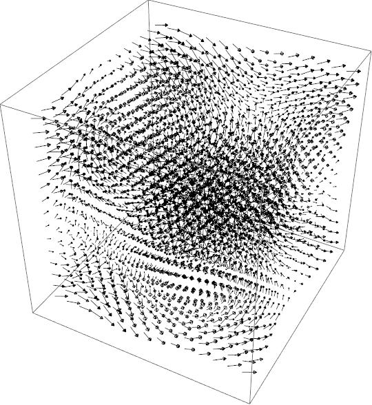
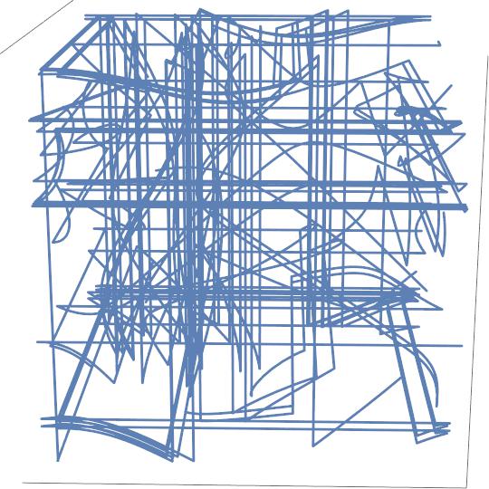
Figure 2: On the left the plot of one arbitrarily chosen vector field in the Beltrami space defined by eq.(7.1). On the right the plots of some of its integral curves in the 3-torus represented as a cube with identified opposite faces.

In order to get a visual appreciation of the difference between Beltrami fields that lead to non-supersymmetric and to supersymmetric $2$-branes we have produced some plots. In figure 2 you see the plot of an arbitrarily chosen vector field in the three-dimensional vector space spanned by (7.1). On the right side a plot of some of its streamlines, namely of its integral curves, is shown.

7.2 The Arnold-Beltrami flux $2$-branes with bosonic symmetry $\mathcal{D}_{n}\ltimes\left[\mathrm{U(1)}\times\mathrm{U(1)}\right]$ and 4 Killing spinors

The next example we consider is a flux $2$-brane that preserves $1/4$ of the original supersymmetry, namely possesses $4$ Killing spinors. As discussed above on general grounds we aspect in this case two translational Killing vectors. This means that eq. (7.13) defining the complete bosonic group of the previously considered solution is replaced by:

$$\mathrm{G}_{bosonic}\,\sim\,\Gamma\,\ltimes\,\left[\mathrm{U(1)}\times\mathrm{U(1)}\right]$$ (7.17)

the two $\mathrm{U(1)}$’s being the continuous translation groups generated by the two additional Killing vectors. The question remains: what is the discrete group $\Gamma$ in this case? We show that using a cubic momentum lattice the answer is:

$$\Gamma\,=\,\mathrm{\mathcal{D}_{4}}$$ (7.18)

where $\mathcal{D}_{4}$ denotes a dihedral group. There is also a second solution based on the hexagonal lattice which yields:

$$\Gamma\,=\,\mathrm{\mathcal{D}_{6}}$$ (7.19)

To see this let us consider the two cases together:

$$\mathfrak{W}_{[4]}\left(\mathbf{X}\right) = \left\{\begin{array}[]{rcl}\mathbf{W}^{1}&=&\mathrm{d}X\,\cos(2\pi Z)-\mathrm{d}Y\,\sin(2\pi Z)\\ \mathbf{W}^{2}&=&-\,\mathrm{d}Y\,\cos(2\pi Z)\,-\,\mathrm{d}X\,\sin(2\pi Z)\\ \mathbf{W}^{3}&=&0\end{array}\right.$$ (7.23)

$$\mathfrak{W}_{[6]}\left(\mathbf{X}\right) = \left\{\begin{array}[]{rcl}\mathbf{W}^{1}&=&\mathrm{d}X\cos\left(\frac{4\pi Z}{\sqrt{3}}\right)-\mathrm{d}Y\sin\left(\frac{4\pi Z}{\sqrt{3}}\right)\\ \mathbf{W}^{2}&=&-\,\mathrm{d}Y\,\cos\left(\frac{4\pi Z}{\sqrt{3}}\right)-\mathrm{d}X\sin\left(\frac{4\pi Z}{\sqrt{3}}\right)\\ \mathbf{W}^{3}&=&0\end{array}\right.$$ (7.27)

Abstractly the dihedral group $\mathrm{\mathcal{D}_{n}}$ can be described by two generators and three relations:

$$\mathrm{\mathcal{D}_{n}}\quad=\quad\left(\mathrm{A},\mathrm{B}\,|\,\mathrm{A}^{n}\,=\,\mathbf{1}\,,\,\mathrm{B^{2}}\,=\,\mathbf{1}\,,\,\left(\mathrm{B\,A}\right)^{2}\,=\,\mathbf{1}\,\right)$$ (7.28)

An explicit representation by means of orthogonal integer valued $3\times 3$ matrices with unit determinant is the following one :

$$\begin{array}[]{ccrclcrcl}\mathrm{\mathcal{D}_{4}}&:&\mathrm{D[A_{4}]}&=&\left(\begin{array}[]{ccc}0&1&0\\ -1&0&0\\ 0&0&1\\ \end{array}\right)&;&\mathrm{D[B]}&=&\left(\begin{array}[]{ccc}-1&0&0\\ 0&1&0\\ 0&0&-1\\ \end{array}\right)\\ \mathrm{\mathcal{D}_{6}}&:&\mathrm{D[A_{6}]}&=&\left(\begin{array}[]{ccc}\frac{1}{2}&\frac{\sqrt{3}}{2}&0\\ -\frac{\sqrt{3}}{2}&\frac{1}{2}&0\\ 0&0&1\\ \end{array}\right)&;&\mathrm{D[B]}&=&\left(\begin{array}[]{ccc}-1&0&0\\ 0&1&0\\ 0&0&-1\\ \end{array}\right)\end{array}$$ (7.29)

The map $\mathrm{D}$ realizes an immersion of the two dihedral groups into the group $\mathrm{SO(3)}$:

$$\mathrm{D}\,:\,\mathrm{\mathcal{D}_{4,6}}\,\hookrightarrow\,\mathrm{SO(3)}$$ (7.30)

The claimed symmetry of the supergravity $2$-brane solution under the group (7.4) stems from the following identities :

$$\mathfrak{W}_{[4,6]}\left(\mathrm{D[A_{4,6}^{-1}]}\cdot\mathbf{X}\right) = \mathrm{D[A_{4,6}]}\cdot\mathfrak{W}_{[4,6]}\left(\mathbf{X}\right)$$

$$\mathfrak{W}_{[4,6]}\left(\mathrm{D[B^{-1}]}\cdot\mathbf{X}\right) = \mathrm{D[B]}\cdot\mathfrak{W}_{[4,6]}\left(\mathbf{X}\right)$$ (7.31)

where the action of the two generators on the torus coordinate is given, this time, by standard matrix multiplication. Hence, just as in the previous case, the complete semidirect product group:

$$G_{bosonic}\,=\,\mathrm{\mathcal{D}_{4,6}}\ltimes\left(\mathrm{U_{X}(1)}\times\mathrm{U_{Y}(1)}\right)$$ (7.32)

is an isometry group for the supergravity solution since the matrices $\mathrm{D[A]}$ and $\mathrm{D[B]}$ are orthogonal and $\mathrm{O(3)}$ is a global symmetry of the supergravity lagrangian.

The inhomogeneous harmonic functions for these brane–solutions are the following ones:

$$\begin{array}[]{rcl}H_{4}(y)&=&1-\frac{1}{48}\lambda^{2}e^{4\pi U}\\ H_{6}(y)&=&1-\frac{1}{48}\lambda^{2}e^{\frac{8\pi}{\sqrt{3}}U}\end{array}$$ (7.33)

and the rest of the solution is obtained from eq.s (6.14-6.18).

Calculating the $\mathfrak{R}$ curvature associated with this solution we find that in any point the rank of its $21$ vielbein components is bounded from above by $12$. Indeed, with little effort, we find a set of $4$ null vectors which surprisingly are null-vectors also of the matrix $\mathfrak{P}$. In this four dimensional subspace the Killing spinor equation is easily integrated by taking all the non vanishing components proportional to $H^{{\textstyle\frac{1}{10}}}$ where $H$ is the inhomogeneous harmonic function. Finally we arrive at the following explicit form of $4$ indipendent Killing spinors:

$$\epsilon_{1}\,=\,H_{4,6}(y)^{{\textstyle\frac{1}{10}}}\,\left(\begin{array}[]{c}0\\ \chi_{4}\\ 0\\ 0\\ 0\\ \chi_{3}\\ 0\\ 0\\ \end{array}\right)\quad;\quad\epsilon_{2}\,=\,H_{4,6}(y)^{{\textstyle\frac{1}{10}}}\,\left(\begin{array}[]{c}\chi_{2}\\ 0\\ 0\\ 0\\ \chi_{1}\\ 0\\ 0\\ 0\\ \end{array}\right)$$ (7.34)

The considered flux-brane solution preserves ${\textstyle\frac{1}{4}}$ of the original supersymmetry.

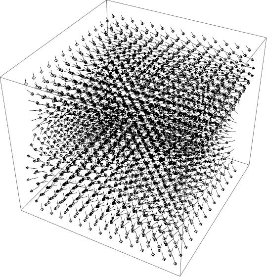
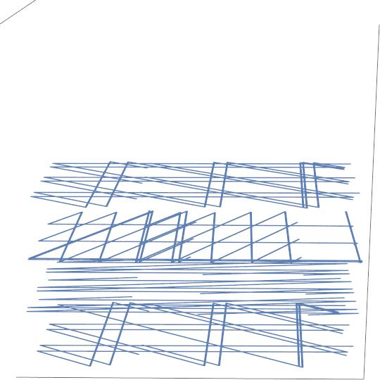
Figure 3: On the left the plot of one arbitrarily chosen vector field in the Beltrami space defined by eq.(7.23). On the right the plots of some of its integral curves in the 3-torus represented as a cube with identified opposite faces. It is evident from the picture that all the integral curves are planar. This a consequence of the two Killing vectors in the $X$ and $Y$ directions.

In the spirit of comparison with the previous case that breaks all supersymmetries, in fig. 3 we have displayed the plot of an arbitrary vector field in the two-dimensional vector space defined by eq. (7.23). The two Killing vectors in the $X$ and $Y$ directions imply that the integral curves are always planar for any element of this vector space and this is quite evident from the figure.

A last comment on this solution concerns a question that might arise in relation with the structure of equations (7.23) and (7.27). One might ask why we should not consider other dihedral groups with $n\neq 4,6$. Indeed it suffices to write the same formulae with a different angle namely:

$$\cos\left[\frac{4\pi}{\sqrt{3}}Z\right]\,\rightarrow\,\cos\left[\frac{2\pi}{\sqrt{\mathbf{m}}}Z\right]$$ (7.35)

The answer why the replacement (7.35) is generically forbidden comes from classical results of crystallography. The coordinates $X,Y,Z$ are supposed to span a torus $\mathbb{R}^{3}/\Lambda$ and in the present case it suffices to consider the planar projection of the lattice $\Lambda$ which produces a tessellation of the plane. Hence the considered dihedral group must be in the list of the so named Wall Paper Point Groups which is finite. Besides $\mathcal{D}_{4}$ and $\mathcal{D}_{6}$ we might still have $\mathcal{D}_{3}$ and $\mathcal{D}_{2}$. We have not explicitly constructed the corresponding supergravity solutions but it is rather clear that they are bound to be completely analogous.

7.3 The Arnold-Beltrami flux $2$-brane with $\left[\mathcal{D}_{4}\otimes\mathbb{Z}_{2}\right]\ltimes\mathrm{U(1)}$ bosonic symmetry and 2 Killing spinors

The next example we consider is a flux $2$-brane that preserves $1/8$ of the original supersymmetry, namely possesses $2$ Killing spinors. On general grounds in this case we expect just one additional Killing vector. This means that eq.s (7.13) and (7.17) defining the complete bosonic groups of the previously considered solutions should now be replaced by:

$$\mathrm{G}_{bosonic}\,\sim\,\Gamma\,\ltimes\,\mathrm{U(1)}$$ (7.36)

the $\mathrm{U(1)}$ factor being the continuous translation group generated by the unique additional Killing vector. The question is the same as in the previous case: what is the discrete group $\Gamma$ here? We show that using a cubic momentum lattice the answer is:

$$\Gamma\,=\,\mathrm{\mathcal{D}_{4}}\times\mathbb{Z}_{2}$$ (7.37)

where $\mathcal{D}_{4}$ denotes once again the dihedral group. To see this let us consider the following triplet of Beltrami vector fields:

$$\widehat{\mathfrak{W}}\left(\mathbf{X}\right) = \left\{\begin{array}[]{rcl}\mathbf{W}^{1}&=&\mathrm{d}X\cos(2\pi Z)-\mathrm{d}Y\sin(2\pi Z)\\ \mathbf{W}^{2}&=&\mathrm{d}X\cos(2\pi Y)+\mathrm{d}X\sin(2\pi Z)+\mathrm{d}Z\sin(2\pi Y)+\mathrm{d}Y\cos(2\pi Z)\\ \mathbf{W}^{3}&=&\mathrm{d}X\sin(2\pi Y)-\mathrm{d}Z\cos(2\pi Y)\end{array}\right.$$ (7.41)

Abstractly the dihedral group $\mathrm{\mathcal{D}_{n}}$ is described in eq. (7.28). In this case, relevant to us is the following representation by means of orthogonal integer valued $3\times 3$ matrices with unit determinant:

$$\begin{array}[]{ccrclcrcl}\mathrm{\mathcal{D}_{4}}&:&\mathrm{D[A]}&=&\left(\begin{array}[]{ccc}0&0&-1\\ 0&1&0\\ 1&0&0\\ \end{array}\right)&;&\mathrm{D[B]}&=&\left(\begin{array}[]{ccc}-1&0&0\\ 0&-1&0\\ 0&0&1\\ \end{array}\right)\end{array}$$ (7.43)

The map $\mathrm{D}$ realizes an immersion of the dihedral group $\mathcal{D}_{4}$ into the group $\mathrm{SO(3)}$:

$$\mathrm{D}\,:\,\mathrm{\mathcal{D}_{4}}\,\hookrightarrow\,\mathrm{SO(3)}$$ (7.44)

If we add the matrix:

$$\mathrm{D[Z]}\,=\,\left(\begin{array}[]{ccc}-1&0&0\\ 0&-1&0\\ 0&0&-1\\ \end{array}\right)$$ (7.45)

which has determinant $-1$ and commutes with both $\mathrm{D[A]}$ and $\mathrm{D[B]}$:

$$\left[\mathrm{D[A]}\,,\,\mathrm{D[Z]}\right]\,=\,\left[\mathrm{D[B]}\,,\,\mathrm{D[Z]}\right]\,=\,0$$ (7.46)

we realize a homomorphic embedding:

$$\mathrm{D}\,:\,\mathcal{D}_{4}\times\mathbb{Z}_{2}\,\hookrightarrow\,\mathrm{O(3)}$$ (7.47)

The claimed symmetry of the supergravity $2$-brane solution under the group (7.37) stems from the following identities that the reader can easily verify:

$$\widehat{\mathfrak{W}}\left(\mathfrak{A}\mathbf{X}\right) = \mathrm{D[A]}\cdot\widehat{\mathfrak{W}}\left(\mathbf{X}\right)$$

$$\widehat{\mathfrak{W}}\left(\mathfrak{B}\mathbf{X}\right) = \mathrm{D[B]}\cdot\widehat{\mathfrak{W}}\left(\mathbf{X}\right)$$

$$\widehat{\mathfrak{W}}\left(\mathfrak{Z}\mathbf{X}\right) = \mathrm{D[Z]}\cdot\widehat{\mathfrak{W}}\left(\mathbf{X}\right)$$ (7.48)

where the action of the three generators on the torus coordinate is defined below:

$$\mathfrak{A}\mathbf{X} = \left\{X,\frac{1}{4}-Z,Y-\frac{3}{4}\right\}$$

$$\mathfrak{B}\mathbf{X} = \{-X,-Y,Z\}$$

$$\mathfrak{Z}\mathbf{X} = \left\{X,Y+\frac{1}{2},Z+\frac{1}{2}\right\}$$ (7.49)

Hence, just as in the previous case, the complete semidirect product group (7.36) is an isometry group for the supergravity solution since the matrices $\mathrm{D[A]}$ and $\mathrm{D[B]}$, $\mathrm{D[Z]}$ are orthogonal and $\mathrm{O(3)}$ is a global symmetry of the supergravity lagrangian.

The inhomogeneous harmonic function for this brane–solution is the following one:

$$\hat{H}(y) = 1-\frac{1}{96}\lambda^{2}e^{4\pi U}\left(4\,-\,2\sin\left[2\pi(Y-Z)\right]+2\sin\left[2\pi(Y+Z)\right]\right)$$ (7.50)

and the rest of the solution is obtained from eq.s (6.14-6.18).

Calculating the $\mathfrak{R}$ curvature associated with this solution we find that in any point the rank of its $21$ vielbein components is bounded from above by $14$. Indeed, with little effort, we find a set of $2$ null vectors which miraculously are null-vectors also of the matrix $\mathfrak{P}$. In such two–dimensional subspace the Killing spinor equation is easily integrated by taking all the non vanishing components proportional to $\hat{H}^{{\textstyle\frac{1}{10}}}(y)$ where $\hat{H}(y)$ is the inhomogeneous harmonic function (7.50). Finally we arrive at the following explicit form of the two linearly independent Killing spinors:

$$\epsilon_{1}\,=\,\hat{H}^{{\textstyle\frac{1}{10}}}(y)\,\left(\begin{array}[]{c}i\chi_{2}\\ 0\\ 0\\ 0\\ i\chi_{1}\\ 0\\ 0\\ 0\\ \end{array}\right)\quad;\quad\epsilon_{2}\,=\,\hat{H}^{{\textstyle\frac{1}{10}}}(y)\,\left(\begin{array}[]{c}0\\ \chi_{2}\\ 0\\ 0\\ 0\\ \chi_{1}\\ 0\\ 0\\ \end{array}\right)$$ (7.51)

In conclusion the considered flux-brane solution preserves ${\textstyle\frac{1}{8}}$ of the original supersymmetry.

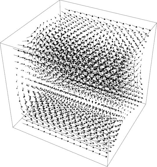
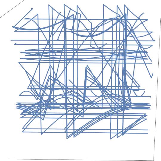
Figure 4: On the left the plot of one arbitrarily chosen vector field in the Beltrami space defined by eq.(LABEL:D4N2). On the right the plots of some of its integral curves in the 3-torus represented as a cube with identified opposite faces.

In the spirit of comparison with the previous case that breaks all supersymmetries, in fig.4 we have displayed the plot of an arbitrary vector field in the three-dimensional vector space defined by eq. (LABEL:D4N2). The Killing vector in the direction $X$ is visually appreciated by the shape of the vector field plot.

Let us finally comment on the structure of the inhomogeneous harmonic function (7.50). For the first time among the considered examples this latter has a non trivial dependence on the $\mathrm{T^{3}}$ torus coordinates. Obviously it has to be a function invariant under the action of the group (7.36). Invariance under the continuous translation of the coordinate $X$ are guaranteed by the fact that $\hat{H}(y)$ does not depend on $X$. The invariance under the discrete part (7.37), whose action on the torus is defined in eq. (7.49) is a priori less obvious, yet it is indeed true, as it can be verified by explicit calculation.

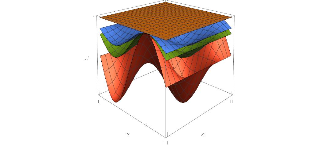
Figure 5: Visualization of the inhomogeneous harmonic function $\hat{H}(y)$ defined by eq.(7.50). The function $\hat{H}$ does not depend on $X$. It depends only on $U,Y,Z$. To visualize it we have plotted the two argument function $H(U_{0},Y,Z)$ defined over the square $Y,Z$, for various values of the constant parameter $U_{0}$. When $U_{0}\,=\,0$ we have the most oscillating surface. As $U_{0}\to-\infty$ the surface plot approaches that of a constant and this corresponds to the asymptotic flatness of the supergravity solution. Note that we have also fixed one reference value of the parameter $\lambda$, explicitly $\lambda=\sqrt{6}$

In fig.5 we present a visualization of this dihedral symmetric function.

8 Uplift of the minimal $D=7$ model to $D=11$ supergravity

In this section we illustrate how the minimal ungauged $D=7$ model, with no vector multiplets, is embedded, as a consistent truncation, in eleven-dimensional supergravity. Consider the latter theory compactified on a 4-torus $\mathrm{T^{4}}$, which yields the maximal seven dimensional supergravity, and write the ${\rm SO}(4)$ symmetry of the internal manifold as: ${\rm SO}(4)={\rm SO}(3)_{+}\times{\rm SO}(3)_{-}$. The minimal $D=7$ supergravity with no vector multiplets describes the truncation of the maximal eleven dimensional theory to the ${\rm SO}(3)_{-}$-singlets. This corresponds to an orbifold reduction from $D=11$ and it is a consistent truncation of the eleven dimensional supergravity.

To show this let us prove that the projection on the dimensionally reduced theory yields the right field content and amount of supersymmetry. Being a restriction to singlets with respect to a symmetry group of the maximal $D=7$ model, it is consistent. Let us denote by hatted indices the $D=11$ ones, so that

Rigid indices: $$\,\,\,\hat{a}=0,\dots,10\,\,;\,\,\,\hat{a}=(a,\,m)\,\,\,;\,\,\,\,a=0,\dots,6\,\,;\,\,\,m=1,2,3,4\,,$$

Coordinate indices: $$\,\,\,\hat{\mu}=0,\dots,10\,\,;\,\,\,\hat{\mu}=(\mu,\,\alpha)\,\,\,;\,\,\,\,\mu=0,\dots,6\,\,;\,\,\,\alpha=1,2,3,4\,,$$

The ${\rm SO}(4)={\rm SO}(3)_{+}\times{\rm SO}(3)_{-}$ vector and spinor-representations, as usual, read:

$$V_{\alpha}\in{\bf\left(\frac{1}{2},\frac{1}{2}\right)}\,\,;\,\,\,\,\xi\in{\bf\left(\frac{1}{2},0\right)+\left(0,\frac{1}{2}\right)}\,.$$ (8.1)

Restricting to the ${\rm SO}(3)_{-}$ - singlets, all tensors with an odd number of $m,\,n$ internal indices are projected out while spinors are halved. In particular the moduli of the internal metric on $\mathrm{T^{4}}$ are frozen to the origin of ${\rm GL}(4,\mathbb{R})/{\rm SO}(4)$, except the determinant of the internal vielbein, which is ${\rm SO}(4)$-invariant and corresponds to the dilaton. After the projection the internal vierbein therefore reads:

$$V_{\alpha}{}^{m}=e^{-\frac{5}{12}\phi}\,\delta_{\alpha}^{m}\,.$$ (8.2)

By the same token the Kaluza-Klein vectors ${\bf B}^{\alpha}_{\mu}$ are truncated out.

The toroidal dimensional reduction of the 3-form yields:

$$\hat{{\bf C}}^{[3]}_{\hat{\mu}\hat{\nu}\hat{\rho}} \rightarrow {\bf B}^{[3]}_{\mu\nu\rho}\,,\,\,{\bf C}^{[2]}_{\mu\nu\alpha}\,,\,\,\,{\bf C}^{[1]}_{\mu\alpha\beta}\,,\,\,\,{\bf C}^{[0]}_{\alpha\beta\gamma}\,.$$ (8.3)

Upon truncation to the ${\rm SO}(3)_{-}$-singlets, the only surviving fields are the 3-form ${\bf B}^{[3]}_{\mu\nu\rho}$ and the projection of the vector fields ${\bf C}^{[1]}_{\mu\alpha\beta}$ on the adjoint representation of ${\rm SO}(3)_{+}$. This projection is effected by restricting to the components of ${\bf C}^{[1]}_{\alpha\beta}\equiv{\bf C}^{[1]}_{\mu\alpha\beta}\,dx^{\mu}$ along the basis $\omega^{(+)\,\Lambda}$ of self-dual 2-forms on the internal $\mathrm{T^{4}}$:

$${\bf C}^{[1]}_{\alpha\beta}|_{{\rm proj}}\,\propto\,\mathcal{A}^{\Lambda}\,\omega^{(+)\,\Lambda}_{\alpha\beta}\,\,;\,\,\,\,\,\star_{{\tiny\mathrm{T^{4}}}}\omega^{(+)\,\Lambda}=\omega^{(+)\,\Lambda}\,\,;\,\,\,d\omega^{(+)\,\Lambda}=0\,.$$ (8.4)

where summation over the repeated $\Lambda$ index is understood and

$$\omega^{(+)\,\Lambda}=J^{(+)\,\Lambda}_{\alpha\beta}\,dy^{\alpha}\wedge dy^{\beta}\,,$$

$J^{\Lambda}$ being the ${\rm SO}(3)_{+}$ generators:

$$J^{(+)\,1}=\left(\begin{array}[]{llll}0&\frac{1}{2}&0&0\\ -\frac{1}{2}&0&0&0\\ 0&0&0&\frac{1}{2}\\ 0&0&-\frac{1}{2}&0\end{array}\right)\,\,;\,\,\,J^{(+)\,2}=\left(\begin{array}[]{llll}0&0&-\frac{1}{2}&0\\ 0&0&0&\frac{1}{2}\\ \frac{1}{2}&0&0&0\\ 0&-\frac{1}{2}&0&0\end{array}\right)\,\,;\,\,\,J^{(+)\,3}=\left(\begin{array}[]{llll}0&0&0&\frac{1}{2}\\ 0&0&\frac{1}{2}&0\\ 0&-\frac{1}{2}&0&0\\ -\frac{1}{2}&0&0&0\end{array}\right)\,.$$ (8.5)

The three components $\mathcal{A}^{\Lambda}\equiv\mathcal{A}^{\Lambda}_{\mu}\,dx^{\mu}$ are the three vector fields of the seven-dimensional minimal model. The dimensionally reduced eleven-dimensional six-form yields the following seven-dimensional fields:

$$\hat{{\bf C}}^{[6]}\,\,\longrightarrow\,\,{{\bf C}}^{[6]},\,{{\bf C}}^{[5]}_{\alpha},\,{{\bf C}}^{[4]}_{\alpha\beta},\,{{\bf C}}^{[3]}_{\alpha\beta\gamma},\,{{\bf C}}^{[2]}_{\alpha_{1}\beta_{1}\alpha_{2}\beta_{2}}\,.$$ (8.6)

Upon truncation, the only surviving fields are a two-form ${\bf B}^{[2]}$, dual to three-form ${\bf B}^{[3]}$, and the three 4-forms $\mathcal{A}^{[4]\Lambda}$ dual to the vector fields, defined as follows:

$${\bf B}^{[2]} \propto \frac{1}{4}\,{\bf C}^{[2]}_{\alpha_{1}\beta_{1}\alpha_{2}\beta_{2}}\,J^{(+)\,\Lambda\,|\alpha_{1}\beta_{1}}J^{(+)\,\Lambda\,|\alpha_{2}\beta_{2}}\,\,;\,\,\,\,\mathcal{A}^{[4]\Lambda}\,\propto\frac{1}{2}\,{\bf C}^{[4]}_{\alpha\beta}\,J^{(+)\,\Lambda\,|\alpha\beta}\,.$$ (8.7)

From the above definitions and the form of the field strength of the eleven dimensional six-form, we find the correct expression of the field strength of ${\bf B}^{[2]}$:

$$\hat{{\bf F}}^{[7]}\equiv d\hat{{\bf C}}^{[6]}+\hat{{\bf F}}^{[4]}\wedge\hat{{\bf C}}^{[3]}+\dots\,\,\rightarrow\,\,\,\,\mathfrak{G}^{[3]}=d{\bf B}^{[2]}+\mathfrak{F}^{\Lambda}\wedge\mathcal{A}^{\Lambda}+\dots$$ (8.8)

Finally let us consider the fermionic sector. The $D=11$ gravitino yields:

$$\hat{\Psi}\, \rightarrow\,\,\Psi_{A},\,\,\Psi_{A^{\prime}},\,\,\Psi_{A\alpha},\,\,\,\Psi_{A^{\prime}\alpha}\,,$$

$$\Psi_{A} \in {\bf\left(\frac{1}{2},0\right)},\,\,\,\Psi_{A^{\prime}}\,\in\,\,{\bf\left(0,\frac{1}{2}\right)}\,,$$

$$\Psi_{A\alpha} \in {\bf\left(\frac{1}{2},0\right)\otimes\left(\frac{1}{2},\frac{1}{2}\right)}={\bf\left(0+1,\,\frac{1}{2}\right)}\,\,;\,\,\,\Psi_{A^{\prime}\alpha}\in{\bf\left(0,\frac{1}{2}\right)\otimes\left(\frac{1}{2},\frac{1}{2}\right)}={\bf\left(\frac{1}{2},\,0+1\right)}$$ (8.9)

The projection singles out the $D=7$ gravitino field $\Psi^{A}$ and the spinors $\chi^{A}$ originating from the ${\bf\left(\frac{1}{2},\,0\right)}$-component of $\Psi_{A^{\prime}\alpha}$:

$$\chi_{A}\,\propto\,\,(\gamma^{\alpha})_{A}{}^{A^{\prime}}\,\Psi_{A^{\prime}\alpha}\,.$$ (8.10)

On the seven-torus $\mathrm{T^{7}}=\mathrm{T^{3}}\times\mathrm{T^{4}}$, product of the $\mathrm{T^{3}}$ in the seven-dimensional space-time and the internal $\mathrm{T^{4}}$, we can write the Englert equation for 3-forms ${\bf Y}^{[3]}$ defined on $\mathrm{T^{7}}$:

$$\star_{{\tiny\mbox{$\mathrm{T^{7}}$}}}d{\bf Y}^{[3]}=\mu\,{\bf Y}^{[3]}\,.$$ (8.11)

Upon restricting to 3-forms of the type ${\bf Y}^{[3]}={\bf Y}^{[1]\,\Lambda}({\bf X})\wedge\omega^{(+)\,\Lambda}$, the Englert equation reduces to the Arnold-Beltrami one considered in the present paper:

$$\star_{{\tiny\mbox{$\mathrm{T^{7}}$}}}d({\bf Y}^{[1]\,\Lambda}\wedge\omega^{(+)\,\Lambda})=\star_{{\tiny\mbox{$\mathrm{T^{3}}$}}}d{\bf Y}^{[1]\,\Lambda}\wedge\star_{{\tiny\mbox{$\mathrm{T^{4}}$}}}\omega^{(+)\,\Lambda}=\mu\,{\bf Y}^{[1]\,\Lambda}\wedge\omega^{(+)\,\Lambda}\,\,\Leftrightarrow\,\,\,\,\star_{{\tiny\mbox{$\mathrm{T^{3}}$}}}d{\bf Y}^{[1]\,\Lambda}=\mu\,{\bf Y}^{[1]\,\Lambda}\,.$$ (8.12)

The dictionary defined in the present section allows to uplift any solution to the minimal $D=7$ supergravity, with no vector multiplets, to eleven dimensions, including the Arnold-Beltrami 2-branes extensively discussed in the previous sections, which describe $M2$-branes with fluxes.

9 Conclusions

In the present paper we have presented the first half of the geometric reconstruction of Minimal $D=7$ supergravity in terms of Free Differential Algebras and rheonomy. Indeed we have completely solved Bianchi identities, fixing the precise form of the supersymmetry transformation rules to all orders in the boson and including higher order terms in the fermion fields.

This general result allowed us to embed Arnold-Beltrami flux $2$-branes into supergravity and study the Killing spinor equation in their background. We have also presented four explicit examples of solutions

1. One solution with no supersymmetry and a discrete symmetry

   $$G_{bosonic}\,=\,\underbrace{\left(\mathrm{O_{24}}\times\mathbb{Z}_{2}\right)}_{\Gamma}\ltimes\underbrace{\left[\mathbb{Z}_{2}\times\mathbb{Z}_{2}\right]}_{\mbox{transl.}}$$ (9.1)

   where $\mathrm{O_{24}}$ denotes the octahedral group.

2. One solution with $4$ Killing spinors and a discrete symmetry:

   $$G_{bosonic}\,=\,\underbrace{\mathrm{\mathcal{D}_{4}}}_{\Gamma}\ltimes\underbrace{\left[\mathrm{U(1)}\times\mathrm{U(1)}\right]}_{\mbox{transl.}}$$ (9.2)

   where $\mathcal{D}_{4}$ denotes the dihedral group of index $4$.

3. One solution with $4$ Killing spinors and a discrete symmetry:

   $$G_{bosonic}\,=\,\underbrace{\mathrm{\mathcal{D}_{6}}}_{\Gamma}\ltimes\underbrace{\left[\mathrm{U(1)}\times\mathrm{U(1)}\right]}_{\mbox{transl.}}$$ (9.3)

   where $\mathcal{D}_{6}$ denotes the dihedral group of index $6$. (We have also advocated that similar solutions should exist for $\mathcal{D}_{2}$ and $\mathcal{D}_{3}$).

4. One solution with 2 Killing spinors and a discrete symmetry

   $$G_{bosonic}\,=\,\underbrace{\left(\mathrm{\mathcal{D}_{4}}\times\mathbb{Z}_{2}\right)}_{\Gamma}\ltimes\underbrace{\mathrm{U(1)}}_{\mbox{transl.}}$$ (9.4)

   where $\mathrm{O_{24}}$ denotes the octahedral group.

The perspectives of further investigations based on the results we have achieved so far are three-fold.

A)

On the one hand we plan to complete our geometrical reconstruction of minimal $D=7$ supergravity, coupled to a generic number of vector fields and including higher order terms in the fermion fields, obtaining the action and after that studying the gaugings of the theory utilizing the method of the embedding tensor [16, 17, 21].

B)

On the other hand, from the point of view of flux $2$-branes we consider the present one as the first step in a logical path of development. We need now to construct the $\kappa$-supersymmetric $2$-brane actions in the background of the brane solutions and study the gauge/gravity correspondence between the $d=3$ gauge theory on the brane world-volume and the bulk supergravity. The discrete symmetries are expected to play a fundamental role in the classification and interactions of the composite operators. Moreover the description of the solutions as $M2$-branes with fluxes in the eleven-dimensional theory suggests that the dual CFT might be related to the ABJM model [22].

C)

A fully-fledged search of supersymmetric flux $2$-branes should be attempted considering all the crystallographic lattices and all their Point Groups. An ambitious aim would be to establish more stringent a priori conditions for the existence of Killing spinors.

D)

Finally it would be interesting to study more general $M2$-branes in the eleven-dimensional supergravity characterized by fluxes which are solutions to the Englert equation (8.11).

Aknowledgements

We are grateful to L. Andrianopoli and R. D’Auria for their contributions to the early stages of the work and for enlightening discussions. One of us (P.F.) is particularly grateful to his friend and collaborator A. Sorin for many important discussions during the whole development of this research project.

Appendix A Detailed derivation of the rheonomic solution of Bianchi identities

In this appendix we present the detailed derivation of the unique rheonomic solution of Bianchi identities of the relevant Free Differential Algebra. The determination of the 24 coefficients mentioned in the main text is the absolute core of the supergravity theory. These numbers decide the explicit form of the supersymmetry transformation rules and implicitly determine the field equations of supergravity, hence its classical dynamics. We already stressed that the very existence of Arnold-Beltrami flux branes critically depends on the precise numerical values of the lagrangian coefficients which on their turn depend, in a one-to-one way, from the coefficients found in the solution of Bianchi identities. Similarly the existence of Killing spinors for given solutions of supergravity, in particular the flux branes studied in this paper, depends on the precise values of 24 coefficients discussed here. Change one of them to a wrong value and the results change not quantitatively but qualitatively. This is not surprising when you remind ourselves that we are talking about the realization of an algebra of transformations. The fascination of supersymmetry and supergravity is that, in this case, the algebra is not kinematics, rather it is the very dynamics of the system.

It follows from these considerations that the calculations presented in this appendix are not marginal rather they are of the utmost relevance. Yet they are extremely tedious. The principle is simple and elegant. Its implementation is desperately tedious, although essential. For this reason these important calculations are relegated to an appendix.

A.1 Rheonomic solution of the Bianchis for the curvatures of degree $p\leq 2$

According to the logic presented in the main test we start by solving completely the Bianchi identities of all the curvatures of degree two or one associated with the standard superalgebra sector of the FDA. As we demonstrate below the set of $19$ parameters $\mbox{coeff}_{\mathrm{Lie}}$ is reduced, after imposing the constraints of these Bianchis to three free parameters, namely $c_{1}$, $g_{1}$ and $\delta$, all the others being fixed in terms of these latter. Let us see how.

A.1.1 Equations from the $3$$\Psi$ sector of the Torsion Bianchi

At the level of $3$$\Psi$ the torsion Bianchi equation (4.1) is very simple. It reads:

$$\overline{\Psi}^{A}\wedge\Gamma^{a}\rho_{A}^{[\Psi\Psi]}\,=\,0$$ (A.1)

where we have named:

$$\rho_{A}^{[\Psi\Psi]} = \,g_{1}\,\Gamma_{m}\,\chi_{A}\,\overline{\Psi}^{C}\wedge\Gamma^{m}\Psi_{C}\,+\,g_{2}\,\Gamma_{mn}\chi_{A}\,\overline{\Psi}^{C}\wedge\Gamma^{mn}\,\Psi_{C}$$ (A.2)

$$-\,g_{3}\,\chi_{B}\,\sigma^{\Lambda|B}_{\phantom{\Lambda|B}A}\,\sigma^{\Lambda|D}_{\phantom{\Lambda|D}C}\,\overline{\Psi}^{C}\wedge\Psi_{D}\,-\,g_{4}\,\Gamma_{pqr}\chi_{B}\,\sigma^{\Lambda|B}_{\phantom{\Lambda|B}A}\,\sigma^{\Lambda|D}_{\phantom{\Lambda|D}C}\,\overline{\Psi}^{C}\wedge\Gamma^{pqr}\Psi_{D}$$

Comparing eq.s (A.1-A.2) with eq.s (3.10-3.11) we realize that eq. (A.1) is nothing else but $\ell_{b}\,=\,0$ which is solved by eq.(3.12) expressing $g_{3}$ and $g_{4}$ in terms of $g_{1,2}$. In this way we have reduced the 19 parameters we are dealing with to seventeen. Let us also note in advance that once eq.(A.1) is satisfied the contribution of $\rho_{A}^{[\Psi\Psi]}$ to the Bianchi equation of $\mathfrak{G}^{[3]}$ (see eq.(4.5)) vanishes a fortiori. This will we important in the sequel.

A.1.2 Equations from the $2$$\Psi$-$1$$V$ sector of the Torsion-Bianchi

Inserting the rheonomic parameterizations (4.9-4.14) into the Bianchi identity (4.1) and keeping only the terms proportional to $2$$\Psi$-$1$$V$, we obtain the following equation:

$$\begin{array}[]{rcl}0&=&-\,R_{\Psi\Psi}^{ab}\wedge V^{b}\,+\,\mathcal{S}^{ab}\wedge V^{b}\\ \end{array}$$ (A.3)

where:

$$R_{\Psi\Psi}^{ab} \equiv \lambda_{1}\,e^{\phi}\,\mathcal{G}^{abc}\,\overline{\Psi}^{A}\wedge\Gamma_{c}\Psi_{A}\,+\,\lambda_{2}\,e^{\phi}\,\mathcal{G}_{pqr}\,\overline{\Psi}^{A}\wedge\Gamma^{abpqr}\Psi_{A}$$ (A.4)

$$\,+\,{\rm i}\,\mu_{1}\,e^{{\textstyle\frac{1}{2}}\phi}\,\mathcal{F}^{\Lambda|ab}\,\sigma^{\Lambda|B}_{\phantom{\Lambda|B}A}\,\overline{\Psi}^{A}\wedge\Psi_{B}\,+\,{\rm i}\,\mu_{2}\,e^{{\textstyle\frac{1}{2}}\phi}\,\mathcal{F}^{\Lambda}_{pq}\,\sigma^{\Lambda|B}_{\phantom{\Lambda|B}A}\,\overline{\Psi}^{A}\wedge\Gamma^{abpq}\,\Psi_{B}$$

$$\mathcal{S}^{ab} = \overline{\Psi}^{A}\,\wedge\,\left(\Gamma^{a}\,\mathcal{M}^{B}_{A}\Gamma^{b}+\Gamma^{ab}\,\mathcal{N}^{B}_{A}\right)\,\Psi_{B}\wedge V^{b}$$ (A.5)

Equation (A.4) is solved by setting first the antisymmetric part of $\mathcal{S}^{ab}$ to zero and then by identifying the symmetric one with $R_{\Psi\Psi}^{ab}$. This yields the following equations on the parameters:

$$\begin{array}[]{rcl}0&=&\kappa_{1}\\ 0&=&\kappa_{2}\\ 0&=&\lambda_{1}+6\left(b_{1}+b_{2}\right)\\ 0&=&\lambda_{2}+\left(b_{1}-b_{2}\right)\\ 0&=&\mu_{1}+2\left(d_{1}-d_{2}\right)\\ 0&=&\mu_{2}+\left(d_{1}+d_{2}\right)\end{array}$$ (A.6)

In this way the seventeen parameters have been reduced to eleven.

A.1.3 Equations from the Gravitino Bianchi at 3$\Psi$-level

If we consider the gravitino Bianchi (4.3) and after insertion of the rheonomic parameterizations (4.9-4.14) we focus on the $3$$\Psi$-sector we obtain the following equation:

$$0 = -\,{\textstyle\frac{1}{4}}\,\Gamma_{ab}\Psi_{A}\wedge R^{ab}_{\Psi\Psi}\,+\,{\textstyle\frac{1}{2}}\,\left(\mathcal{M}^{B}_{A}\Gamma_{b}+\Gamma_{b}\,\mathcal{N}^{B}_{A}\right)\,\Psi_{B}\wedge\overline{\Psi}^{C}\wedge\Gamma^{b}\Psi_{C}$$ (A.7)

$$-\,g_{1}\,\Gamma_{m}\,\mathcal{P}^{D}_{A}\,\Psi_{D}\,\overline{\Psi}^{C}\wedge\Gamma^{m}\Psi_{C}\,-\,g_{2}\,\Gamma_{mn}\mathcal{P}^{D}_{A}\,\Psi_{D}\,\overline{\Psi}^{C}\wedge\Gamma^{mn}\,\Psi_{C}$$

$$+\,g_{3}\,\mathcal{P}^{E}_{B}\,\Psi_{E}\,\sigma^{\Lambda|B}_{\phantom{\Lambda|B}A}\,\sigma^{\Lambda|D}_{\phantom{\Lambda|D}C}\,\overline{\Psi}^{C}\wedge\Psi_{D}\,+\,g_{4}\,\Gamma_{pqr}\mathcal{P}^{E}_{B}\,\Psi_{E}\,\sigma^{\Lambda|B}_{\phantom{\Lambda|B}A}\,\sigma^{\Lambda|D}_{\phantom{\Lambda|D}C}\,\overline{\Psi}^{C}\wedge\Gamma^{pqr}\Psi_{D}$$

Separate cancellation of the terms proportional to $\mathcal{G}_{abc}$, $\mathcal{F}^{\Lambda}_{ab}$ and $\Phi_{a}$ imposes on the parameters a set of conditions which together with those found in the previous two subsections yields the following result:

$$b_{1} = 16\,c_{1}\,g_{2}$$

$$b_{2} = \frac{4}{3}\,c_{1}\left(g_{1}-2\,g_{2}\right)$$

$$d_{1} = -32\,c_{2}\,g_{2}$$

$$d_{2} = \frac{4}{3}\,c_{2}\,\left(g_{1}+10\,g_{2}\right)$$

$$g_{3} = \frac{1}{6}\left(-5\,g_{1}-14\,g_{2}\right)$$

$$g_{4} = \frac{1}{36}\left(2\,g_{2}-g_{1}\right)$$

$$\kappa_{1} = 0$$

$$\kappa_{2} = 0$$

$$\lambda_{1} = -8c_{1}\,\left(g_{1}+10\,g_{2}\right)$$

$$\lambda_{2} = \frac{4}{3}c_{1}\left(g_{1}-14\,g_{2}\right)$$

$$\mu_{1} = \frac{8}{3}\,c_{2}\,\left(g_{1}+34\,g_{2}\right)$$

$$\mu_{2} = -\frac{4}{3}\,c_{2}\,\left(g_{1}-14\,g_{2}\right)$$ (A.8)

In this way the set of free coefficients among the 19 comprised in $\mbox{coeff}_{\mathrm{Lie}}$ is reduced to seven, namely:

$$\{a_{1},\,c_{1},\,c_{2},\,c_{3},\,g_{1},\,g_{2},\,\delta\}$$ (A.9)

A.1.4 Equation for $c_{3}$ from the dilaton Bianchi

The coefficient $c_{3}$ is easily and immediately determined from the dilaton Bianchi (4.7), upon insertion of the rheonomic parameterization (4.13). We immediately obtain:

$$c_{3}\,=\,{\textstyle\frac{1}{2}}$$ (A.10)

A.1.5 Equations from the $2$$\Psi$-$1$$V$ sector of the $\mathfrak{F}^{\Lambda}$-Bianchi

Inserting the rheonomic parameterizations (4.9-4.14) into the Bianchi identity (4.4) and keeping only the terms proportional to $2$$\Psi$-$1$$V$, we obtain the following equation:

$$0 = -\,\mathcal{F}^{\Lambda}_{ab}\overline{\Psi}^{A}\wedge\Gamma^{a}\Psi_{A}\wedge V^{b}\,+\,{\rm i}\,a_{1}\,e^{-{\textstyle\frac{1}{2}}\phi}\,\sigma^{\Lambda|B}_{\phantom{\Lambda|B}A}\,\overline{\Psi}^{A}\wedge\Gamma_{a}\mathcal{P}^{C}_{B}\Psi_{C}\wedge V^{a}$$

$$+{\rm i}\,e^{-{\textstyle\frac{1}{2}}\phi}\,\sigma^{\Lambda|B}_{\phantom{\Lambda|B}A}\,\overline{\Psi}^{A}\left(\mathcal{M}_{B}^{C}\,\Gamma_{a}+\Gamma_{a}\,\mathcal{N}_{B}^{C}\right)\Psi_{C}\wedge V^{a}\,+\,{\rm i}{\textstyle\frac{1}{4}}\,e^{-{\textstyle\frac{1}{2}}\phi}\,\sigma^{\Lambda|B}_{\phantom{\Lambda|B}A}\,\Phi_{a}\wedge\overline{\Psi}^{A}\,\wedge\,\Psi_{B}\wedge V^{a}$$

Imposing the cancellation of all structures we obtain the following equations on the coefficients:

$$a_{1} = -\,\frac{1}{2}$$

$$c_{2} = \frac{7}{24-64\,g_{1}}$$

$$g_{2} = \frac{1}{112}\left(8\,g_{1}\,-\,3\right)$$ (A.12)

In this way the seven free parameters mentioned in eq. (A.9) are reduced to the three mentioned at the beginning of this subsection

A.1.6 Equations from the 3$\Psi$-level of the $\mathfrak{F}^{\Lambda}$ curvature

At the 3$\Psi$-level the Bianchi identity of the $\mathfrak{F}^{\Lambda}$ curvature, namely eq. (4.4), reduces to the following statement:

$$0 = {\rm i}\,{\textstyle\frac{1}{4}}\,e^{-{\textstyle\frac{1}{2}}\,\phi}\,\overline{\Psi}^{C}\,\chi_{C}\,\wedge\,\overline{\Psi}^{A}\,\wedge\,\sigma^{\Lambda|B}_{A}\,\Psi_{B}\,+\,{\rm i}\,e^{-{\textstyle\frac{1}{2}}\,\phi}\,\overline{\Psi}^{A}\,\wedge\,\sigma^{\Lambda|B}_{A}\,\rho_{B}^{[\Psi\Psi]}$$ (A.13)

$$+\,{\rm i}\,{\textstyle\frac{1}{2}}\,a_{1}\,e^{-{\textstyle\frac{1}{2}}\,\phi}\,\sigma^{\Lambda|B}_{\phantom{\Lambda|B}A}\,\overline{\Psi}^{A}\Gamma_{a}\,\chi_{B}\,\wedge\,\overline{\Psi}^{C}\wedge\Gamma^{a}\Psi_{C}$$

which, surprisingly imposes no new constraint and it is identically satisfied by the set of parameters satisfying all the previous constraints, namely:

$$\begin{array}[]{rclcrclcrcl}a_{1}&=&-{\textstyle\frac{1}{2}}&;&b_{1}&=&\frac{c_{1}}{7}\left(-3+8\,g_{1}\right)&;&b_{2}&=&\frac{c_{1}}{7}\left(1+16\,g_{1}\right)\\ c_{1}&=&c_{1}&;&c_{2}&=&\frac{7}{24-64\,g_{1}}&;&c_{3}&=&{\textstyle\frac{1}{2}}\\ d_{1}&=&{\textstyle\frac{1}{4}}&;&d_{2}&=&\frac{5-32\,g_{1}}{16(-3+8\,g_{1})}&;&g_{1}&=&g_{1}\\ g_{2}&=&{\textstyle\frac{1}{112}}(-3+8\,g_{1})&;&g_{3}&=&{\textstyle\frac{1}{16}}-g_{1}&;&g_{4}&=&-\,{\textstyle\frac{1}{672}}\left(1+16\,g_{1}\right)\\ \kappa_{1}&=&0&;&\kappa_{2}&=&0&;&\lambda_{1}&=&-\,\frac{3}{7}\,c_{1}\,\left(-5+32\,g_{1}\right)\\ \lambda_{2}&=&\frac{c_{1}}{2}&;&\mu_{1}&=&\frac{17-64\,g_{1}}{8\left(-3+8\,g_{1}\right)}&;&\mu_{2}&=&\frac{7}{16\left(-3+8\,g_{1}\right)}\\ \delta&=&\delta&;&\hbox{}\hfil&\hbox{}\hfil&\hbox{}&;&\hbox{}\hfil&\hbox{}\hfil&\hbox{}\\ \end{array}$$ (A.14)

A.2 Solving the Bianchis for curvatures of degree $p=3,4$

Having completely solved the Bianchi identities for the curvatures of degree $p\leq 2$ we have been left with three parameters $\delta,c_{1}$ and $g_{1}$ that parameterize all the others according to eq.(A.14). In the background of such parameterized curvatures we consider the Bianchi identities of the higher degree curvatures.

We begin with the Bianchi of the $\mathfrak{G}^{[3]}$ form corresponding to the formulation of [2] and [3].

A.2.1 Equations from the $2$$\Psi$-$2$$V$ sector of the $\mathfrak{G}^{[3]}$-Bianchi

Inserting the rheonomic parameterizations (4.9-4.14) into the Bianchi identity (4.5) and keeping only the terms proportional to $2$$\Psi$-$2$$V$, we obtain the following equation:

$$\begin{array}[]{rcl}0&=&\left(\lambda_{1}q-{\textstyle\frac{3}{2}}\right)\,G_{abc}\,\overline{\Psi}^{A}\wedge\Gamma^{a}\Psi_{A}\wedge V^{b}\wedge V^{c}\,+\,\lambda_{2}q\,G_{pqr}\,\overline{\Psi}^{A}\wedge\Gamma^{pqrab}\Psi_{A}\wedge V_{a}\wedge V_{b}\\ \hbox{}\hfil&\hbox{}\hfil&+\,{\rm i}\left(\mu_{1}q+1\right)\,e^{-{\textstyle\frac{1}{2}}\phi}\,\mathcal{F}^{\Lambda}_{ab}\,\sigma^{\Lambda|B}_{\phantom{\Lambda|B}A}\,\overline{\Psi}^{A}\wedge\Psi_{B}\wedge V^{a}\wedge V^{b}\\ \hbox{}\hfil&\hbox{}\hfil&+\,{\rm i}\mu_{2}q\,e^{-{\textstyle\frac{1}{2}}\phi}\,\mathcal{F}^{\Lambda}_{pq}\,\sigma^{\Lambda|B}_{\phantom{\Lambda|B}A}\,\overline{\Psi}^{A}\wedge\Gamma^{pqab}\Psi_{B}\wedge V_{a}\wedge V_{b}+{\textstyle\frac{1}{2}}\,e^{-\phi}\,\Phi_{a}\,\overline{\Psi}^{A}\wedge\Gamma_{b}\Psi_{A}\wedge V^{a}\wedge V^{b}\\ \hbox{}\hfil&\hbox{}\hfil&-(q-1)\,e^{-\phi}\,\overline{\Psi}^{A}\wedge\left(\Gamma_{a}\,\mathcal{M}^{B}_{A}\,\Gamma_{b}+\Gamma_{ab}\mathcal{N}^{B}_{A}\right)\Psi_{B}\wedge V^{a}\wedge V^{b}\\ &\hbox{}\hfil&+\,a_{2}\,e^{-\phi}\,\overline{\Psi}^{A}\wedge\Gamma_{ab}\,\mathcal{P}^{B}_{A}\Psi_{B}\wedge V^{a}\wedge V^{b}\end{array}$$ (A.15)

Imposing the identical cancellation of all type of terms and previously eliminating the parameters $\lambda_{1,2},\mu_{1,2}$ via eq.s (A.6) we obtain the following equations on the remaining parameters:

$$\begin{array}[]{rcl}0&=&-3\left(4b_{1}+4b_{2}+4a_{2}c_{1}+1\right)\\ 0&=&-b_{1}+b_{2}+a_{2}c_{1}\\ 0&=&4a_{2}c_{3}+1\\ 0&=&a_{2}c_{2}-(q-2)\left(d_{1}+d_{2}\right)\\ 0&=&2a_{2}c_{2}-2d_{1}+2d_{2}+1\end{array}$$ (A.16)

Combining the above equations with those in eq.(A.14) we obtain the final solution for the 21 parameters in eq. (4.22). Such a solution, which is displayed below, depends on a free parameter that we have localized in $g_{1}$. All values of $g_{1}$ are permitted except ${\textstyle\frac{3}{8}}$ for which the solution becomes singular:

$$\begin{array}[]{rclcrclcrcl}a_{1}&=&-{\textstyle\frac{1}{2}}&;&b_{1}&=&-{\textstyle\frac{1}{8}}&;&b_{2}&=&-\,{\textstyle\frac{1}{8}}+\frac{7}{48-128\,g_{1}}\\ c_{1}&=&\frac{7}{24-64\,g_{1}}&;&c_{2}&=&\frac{7}{24-64\,g_{1}}&;&c_{3}&=&{\textstyle\frac{1}{2}}\\ d_{1}&=&{\textstyle\frac{1}{4}}&;&d_{2}&=&-\,{\textstyle\frac{1}{4}}+\frac{7}{48-128\,g_{1}}&;&g_{1}&=&g_{1}\\ g_{2}&=&{\textstyle\frac{1}{112}}(-3+8\,g_{1})&;&g_{3}&=&{\textstyle\frac{1}{16}}-g_{1}&;&g_{4}&=&-\,{\textstyle\frac{1}{672}}\left(1+16\,g_{1}\right)\\ \kappa_{1}&=&0&;&\kappa_{2}&=&0&;&\lambda_{1}&=&\frac{3}{8}\,\left(4+\frac{7}{-3+8\,g_{1}}\right)\\ \lambda_{2}&=&\frac{7}{48-128\,g_{1}}&;&\mu_{1}&=&-1+\frac{7}{24-64\,g_{1}}&;&\mu_{2}&=&\frac{7}{16\left(-3+8\,g_{1}\right)}\\ \delta&=&1&;&q&=&1&;&a_{2}&=&-{\textstyle\frac{1}{2}}\\ \end{array}$$ (A.17)

It is now very interesting to compare the solution (A.17) with the supersymmetry transformation rules derived by the authors of [3]. A comparison at the level of absolute values of the coefficients is very laborius since it involves the normalization of the various fields, but there is a simple and very significant test that is intrinsic and normalization independent. We refer to the ratio of the coefficients $b_{1}/b_{2}$ and $d_{1}/d_{2}$ that appear in the gravitino curvature and that dictate the form of the gravitino transformation rule. These ratios cannot be deformed by changing the normalization of any field and hence are an intrinsic property of the susy algebra, i.e. of the rheonomic parameterizations. Comparing with eq.(2.9) of [3] we see that according to these authors the two ratios are predicted to be:

$$\frac{b_{1}}{b_{2}}\,=\,5\quad;\quad\frac{d_{1}}{d_{2}}\,=\,-\,\frac{5}{3}$$ (A.18)

It is non trivial and reassuring that the two above equations for the parameter $g_{1}$ are consistent and admit the common solution:

$$g_{1}\,=\,-\frac{11}{64}$$ (A.19)

In this way we have reconstructed the formulation by Bergshoeff et al of minimal $D=7$ supergravity, but we have also learned that it admits a non trivial deformation encoded in the parameter $g_{1}$. Obviously the parameter $g_{1}$ could not be seen by the authors of [3] since they did not consider quadratic fermion terms in the transformation rules of the fermions and implicitly fixed a choice of $g_{1}$ adopting a certain relative strength of the kinetic terms in the lagrangian.

A.2.2 Equations from the $3$$\Psi$ sector of the $\mathfrak{G}^{[4]}$ Bianchi

In the case we utilize the 3-form formulation we have to satisfy also the Bianchi identity of the $\mathfrak{G}^{[4]}$-curvature. This latter has a $3$$\Psi$-sector that differently from the case of the 2-form is not identically satisfied by the solution of torsion Bianchi equation. This sector yields the following equation:

$$0 = {\rm i}\,e^{-{\theta}\phi}\,\left(\overline{\Psi}^{A}\wedge\Gamma_{ab}\rho^{[\Psi\Psi]}_{A}\,+\,\frac{3}{2}\,w\,\overline{\Psi}^{A}\wedge\Gamma_{abc}\chi_{A}\wedge\overline{\Psi}^{B}\wedge\Gamma^{c}\Psi_{B}\right.$$ (A.20)

$$\left.+\frac{\theta}{2}\,\overline{\Psi}^{A}\wedge\chi_{A}\wedge\overline{\Psi}^{B}\wedge\Gamma_{ab}\Psi_{B}\right)\wedge V^{a}\wedge V^{b}$$

which imposes the following two constraints on the coefficients:

$$\frac{6}{7}\,-\,12\,w\,-\,\frac{128}{7}\,g_{1} = 0$$

$$\frac{6}{7}\,+\,12\,\theta\,-\,\frac{128}{7}\,g_{1} = 0$$ (A.21)

which are solved by the following conditions:

$$w\,=\,-\,\frac{\theta}{3}\quad;\quad g_{1}\,=\,\frac{1}{64}\left(3\,+\,14\,\theta\right)$$ (A.22)

A.2.3 Equations from the $2$$\Psi$ sector of the $\mathfrak{G}^{[4]}$ Bianchi

At this point we have still to consider the $2$$\Psi$ sector of the $\mathfrak{G}^{[4]}$-Bianchi which yields the following equation:

$$\begin{array}[]{rcl}0&=&-2\,\nu\,e^{(1-\theta)\phi}\,\varepsilon_{pqrabcd}\,G^{pqr}\,\overline{\Psi}^{A}\wedge\Gamma^{d}\Psi_{A}\wedge V^{a}\wedge V^{b}\wedge V^{c}\\ \hbox{}\hfil&\hbox{}\hfil&+{\rm i}\left(e^{-\theta\phi}\,\overline{\Psi}^{A}\wedge\left(\Gamma_{ab}\,\mathcal{M}^{B}_{A}\,\Gamma_{c}+\Gamma_{abc}\mathcal{N}^{B}_{A}\right)\Psi_{B}\wedge V^{a}\wedge V^{b}\wedge V^{c}\right.\\ &\hbox{}\hfil&\left.+\,w\,e^{-\theta\phi}\,\overline{\Psi}^{A}\wedge\Gamma_{abc}\,\mathcal{P}^{B}_{A}\Psi_{B}\wedge V^{a}\wedge V^{b}\wedge V^{c}\right)-\frac{i}{2}\,e^{-\theta\phi}\,\Phi_{c}\,\overline{\Psi}^{A}\Gamma_{ab}\Psi_{A}\wedge V^{a}\wedge V^{b}\wedge V^{c}\end{array}$$ (A.23)

It is very much reassuring that all the other structures cancel identically in eq.(A.23) upon the use of the coefficients that we have already determined and that those involving $G^{pqr}$ cancel also identically upon fixing the following value for the parameter $\nu$:

$$\nu\,=\,\frac{1}{12}$$ (A.24)

In this way we have completely solved in a rheonomic way the Bianchi identities involving both the three-form and the four-form curvatures whose space-time field strengths are dual to each other. Altogether we have found the following set of coefficients parameterized by the single parameter theta:

$$\begin{array}[]{llllllllllll}a_{1}&=&-\frac{1}{2}&;&a_{2}&=&-\frac{1}{2}&;&b_{1}&=&-\frac{1}{8}&\\ b_{2}&=&\frac{2\theta+1}{24-16\theta}&;&c_{1}&=&\frac{1}{3-2\theta}&;&c_{2}&=&\frac{1}{3-2\theta}&\\ c_{3}&=&\frac{1}{2}&;&d_{1}&=&\frac{1}{4}&;&d_{2}&=&\frac{1-2\theta}{8\theta-12}&\\ g_{1}&=&\frac{1}{64}(14\theta+3)&;&g_{2}&=&\frac{1}{128}(2\theta-3)&;&g_{3}&=&\frac{1}{64}(1-14\theta)&\\ g_{4}&=&\frac{1}{384}(-2\theta-1)&;&\kappa_{1}&=&0&;&\kappa_{2}&=&0&\\ \lambda_{1}&=&\frac{3}{2}+\frac{3}{2\theta-3}&;&\lambda_{2}&=&\frac{1}{6-4\theta}&;&\mu_{1}&=&\frac{1}{3-2\theta}-1&\\ \mu_{2}&=&\frac{1}{4\theta-6}&;&\delta&=&1&;&w&=&-\frac{\theta}{3}&\\ q&=&1&;&\nu&=&\frac{1}{12}&;&\theta&=&\theta&\end{array}$$

The solution as usual is multiply checked since the constraints are many more than the parameters that can be fixed.

Appendix B Constraints on the rheonomic action coefficients from comparison with $TPvN$ and the flux brane action

We have shown that the second order bosonic lagrangian of [1] is identical, after appropriate rescalings to the flux-brane lagrangian (2.10). On the other hand the supersymmetry transformations of [1] agree, after appropriate rescalings, with those issuing from the rheonomic parameterization of the Bianchi identities presented in the previous sections. Ergo the bosonic sector of the action of $D=7$ supergravity streaming from the rheonomic approach must map, after the rescalings (5.13), into the flux-brane lagrangian (2.10). This happens if certain relations on the coefficients $f_{i}$ of the bosonic action (4.29) are satisfied. In the present section we derive these constraints postponing to a forthcoming publication their verification within the full determination of all the coefficients of the full rheonomc action.

Discarding the gravitino 1-forms and the dilatino $\chi$ the action $\mathcal{L}^{ungauged}_{Bkin}$ reduces to:

$$\mathcal{L}^{ungauged}_{Bose} = f_{1}\,\mathfrak{R}^{a_{1}a_{2}}\wedge V^{a_{3}}\wedge\dots\wedge V^{a_{7}}\,\epsilon_{a_{1}\dots a_{7}}$$

$$\,+\,f_{2}\,\Phi^{a_{1}}\,\mathrm{d}\phi\,\wedge V^{a_{2}}\wedge\dots\wedge V^{a_{7}}\,\epsilon_{a_{1}\dots a_{7}}$$

$$+f_{3}\,e^{\phi}\,\mathcal{F}^{\Lambda|a_{1}a_{2}}\,\mathfrak{F}^{\Lambda}\,\wedge V^{a_{3}}\wedge\dots\wedge V^{a_{7}}\,\epsilon_{a_{1}\dots a_{7}}$$

$$+\,f_{4}\,\mathcal{G}_{abc}\,\mathfrak{G}^{[4]}\wedge V^{a}\wedge V^{b}\wedge V^{c}\,+\,f_{5}\,\mathfrak{G}^{[3]}\wedge\mathfrak{G}^{[4]}$$

$$+\,\left(-\,360f_{2}\,\Phi^{a}\,\Phi_{a}\,-\,120\,f_{3}\,e^{\phi}\,\mathcal{F}^{\Lambda|ab}\mathcal{F}^{\Lambda}_{ab}-6\,f_{4}\,e^{2\phi}\,\mathcal{G}_{abc}\,\mathcal{G}^{abc}\right)\,\mathrm{Vol}_{7}$$

$$\mathrm{Vol}_{7} \equiv \frac{1}{7!}\,\epsilon_{a_{1}\dots a_{7}}\,V^{a_{1}}\wedge\dots\wedge V^{a_{7}}$$ (B.1)

Eliminating the auxiliary fields that realize the first order formalism we can rewrite the second order form of the above lagrangian which reads as follows:

$$L_{Bose}^{ungauged} = \mbox{det}V\,\left(240\,f_{1}\,R[g]\,+\,360\,f_{2}\partial^{\mu}\phi\,\partial_{\mu}\phi\,+\,6\,f_{4}e^{-2\phi}\,\mathcal{G}_{\lambda\mu\nu\rho}\,\mathcal{G}^{\lambda\mu\nu\rho}\,\right.$$ (B.2)

$$\left.+\,120\,f_{3}\,e^{{\textstyle\frac{1}{2}}\,\phi}\,\mathcal{F}^{\Lambda|\mu\nu}\,\mathcal{F}^{\Lambda}_{\mu\nu}\right)\,d^{7}x\,+\,f_{5}\,\mathfrak{G}^{[4]}\wedge\mathfrak{G}^{[3]}$$

where $\mathcal{G}_{\lambda\mu\nu\rho}$ are the holonomic components of the field curvature $\mathfrak{G}^{[4]}$:

$$\mathfrak{G}^{[4]}\,\equiv\,\mathrm{d}\mathbf{B}^{[3]}\,=\,\mathcal{G}_{\lambda\mu\nu\rho}\,dx^{\lambda}\wedge dx^{\mu}\wedge dx^{\nu}\wedge dx^{\rho}$$ (B.3)

The anholonomic components of the same tensor with flat indices is related to $\mathcal{G}_{abc}$ by the already established relation:

$$\mathcal{G}_{a_{1}a_{2}a_{3}a_{4}}\,=\,\frac{1}{12}\,e^{2\phi}\,\epsilon_{a_{1}a_{2}a_{3}a_{4}pqr}\,\mathcal{G}^{pqr}$$ (B.4)

An alternative way of writing the same lagrangian which is quite convenient while dealing with the equation of motion is the following one:

$$L_{Bose}^{ungauged} = \mbox{det}V\,\left(240\,f_{1}\,\mathcal{R}[g]\,+\,360\,f_{2}\partial^{\mu}\phi\,\partial_{\mu}\phi\,\right)d^{7}x$$ (B.5)

$$+\,{\textstyle\frac{1}{4}}\,f_{4}e^{-2\phi}\,\mathfrak{G}^{[4]}\wedge\star\mathfrak{G}^{[4]}\,+\,f_{5}\,\mathfrak{G}^{[4]}\wedge\mathfrak{G}^{[3]}\,+\,60\,f_{3}\,e^{\phi}\,{\mathfrak{F}}^{\Lambda}\wedge\star\mathfrak{F}^{\Lambda}$$

Recalling that $\mathfrak{G}^{[3]}\,=\,\mathrm{d}\mathbf{B}^{[3]}\,+\,{\mathfrak{F}}^{\Lambda}\wedge\mathcal{A}^{\Lambda}$ the field equations for the one-forms $\mathcal{A}^{\Lambda}$ and the three form $\mathbf{B}^{[3]}$ can be respectively written as follows:

$$\mathrm{d}\star\mathfrak{F}^{\Lambda} = \frac{f_{5}}{60\,f_{3}}\,{\mathfrak{F}}^{\Lambda}\wedge\mathfrak{G}^{[4]}$$ (B.6)

$$\mathrm{d}\star\left[e^{-2\phi}\,\star\mathfrak{G}^{[4]}\right] = 2\,\mathfrak{F}^{\Lambda}\wedge\mathfrak{F}^{\Lambda}$$ (B.7)

while the equation for the dilaton takes the following form:

$$\Box\,\phi\,\mathrm{Vol}_{7}=\,-\,\frac{f_{4}}{1440\,f_{2}}e^{-2\phi}\,\mathfrak{G}^{[4]}\wedge\star\mathfrak{G}^{[4]}\,+\,\frac{f_{3}}{12\,f_{2}}\,e^{\phi}\,{\mathfrak{F}}^{\Lambda}\wedge\star\mathfrak{F}^{\Lambda}$$ (B.8)

The Einstein equation for the metric can be finally written as follows:

$$\left(\mbox{Ric}_{\mu\nu}\,-\,{\textstyle\frac{1}{2}}\,g_{\mu\nu}\,\mathcal{R}\right) = T^{\phi}_{\mu\nu}\,+\,T^{\mathcal{G}}_{\mu\nu}$$

$$T^{\phi}_{\mu\nu} = -\,{\textstyle\frac{3}{2}}\,\frac{f_{2}}{f_{1}}\left(\partial_{\mu}\phi\,\partial_{\nu}\phi\,-\,{\textstyle\frac{1}{2}}\,g_{\mu\nu}\,\partial^{\rho}\phi\,\partial_{\rho}\phi\right)$$ (B.9)

$$T^{\mathcal{G}}_{\mu\nu} = -\,{\textstyle\frac{1}{10}}\,\frac{f_{4}}{f_{1}}\,\left(\mathcal{G}_{\mu...}\,\mathcal{G}_{\nu}^{\phantom{\nu}...}\,-\,{\textstyle\frac{1}{8}}\,g_{\mu\nu}\,\mathcal{G}_{....}\,\mathcal{G}^{....}\right)$$ (B.10)

where the dots denote saturated indices.

B.1 Embedding the $2$-brane solution in supergravity

In order to embed the two brane solution discussed in section 2 into Minimal $D=7$ Supergravity one has to bring, by means of field redefinitions, the lagrangian (B.5) to the standard form of (2.1) or even (2.10) if we want to switch on Arnold Beltrami fluxes. Let us divide the task in two parts. First we show that we can always embed the brane solution without fluxes, next we consider the embedding of the flux brane solution and we work out the condition on the lagrangian coefficients that has to be satisfied in order for such an embedding to be feasible.

B.1.1 Matching with the pure brane action

The first thing to do in order to compare (B.5) with (2.1) is to truncate the gauge fields $\mathcal{A}^{\Lambda}$ by setting them to zero, which is a consistent operation in the field equations (B.6),(B.7) and (B.8). Secondly we set the coefficient of the Einstein term to the following value:

$$f_{1}\,=\,-\,\frac{1}{5!2!}\,=\,-\,\frac{1}{240}$$ (B.11)

This is always possible since the overall constant in front of the lagrangian is a free parameter and supersymmetry fixes all the other coefficients in terms of $f_{1}$. In the sequel the other coefficients $\hat{f}_{2},\hat{f}_{3},\hat{f}_{4}$ are meant to attain the value predicted by supersymmetry when the Einstein term is canonically normalized as in equation(B.11):

$$\hat{f}_{2}\,=\,\frac{f_{2}}{-240\,f_{1}}\quad;\quad\hat{f}_{3}\,=\,\frac{f_{3}}{-240\,f_{1}}\quad;\quad\hat{f}_{4}\,=\,\frac{f_{4}}{-240\,f_{1}}$$ (B.12)

The second and third steps consists of a rescaling of the dilaton and of the $\mathfrak{G}^{[4]}$-form. We utilize the identifications provided by eq. (5.13), with the request that after rescaling the kinetic terms become canonical namely:

$$6\,\hat{f}_{4}\,\tau^{2}\,=\,\frac{1}{24}\,\hat{f}_{4}\,=\,\frac{1}{96}\quad;\quad 360\,\hat{f}_{2}\,\lambda^{2}\,=\,360\,\hat{f}_{2}\,\frac{2}{5}\,=\,-\,\frac{1}{4}$$ (B.13)

The consistency of the above equations implies that when $f_{1}$ is negative, $f_{2}<0$ should also be negative and $f_{4}>0$ should instead be positive. This requirement, although we have not yet fixed the coefficients by supersymmetry, should be in any way respected, since it corresponds to positivity of the energy in the mostly minus conventions for the metric signature. In this way we find:

$$\hat{f}_{4} = \frac{1}{4}$$ (B.14)

$$\hat{f}_{2} = -\,\frac{1}{576}$$ (B.15)

B.2 Matching with the flux brane action

In order for the flux brane action (2.10) to match the bosonic action of supergravity further conditions have to be satisfied by the action coefficients. We presently derive them. First we consider the rescaling necessary to bring the kinetic term of the gauge fields $\mathcal{A}^{\mu}$ to the normalization used in eq.(2.10). Referring to eq.(5.13) we see that the necessary rescaling is given by:

$$\sigma^{2}\,=\,-\,\frac{f_{1}}{4\,f_{3}}\,\omega$$ (B.16)

Then we can evaluate, in terms of $f_{5}$ the value of the parameter $\kappa$ appearing in the lagrangian (2.10). We find the condition:

$$\kappa\,=\,\frac{f_{5}}{240\,f_{1}}\,\tau\,\sigma^{2}\,=\,\frac{\omega}{384}$$ (B.17)

Utilizing $\tau\,=\,{\textstyle\frac{1}{12}}$, the identification (B.16) and:

$$f_{5}\,=\,-\,f_{4}\,=\,\frac{1}{4}\times(240\,f_{1})$$ (B.18)

we get:

$$f_{3}\,=\,2\,f_{1}\quad\Rightarrow\quad\hat{f}_{3}\,=\,-\,\frac{1}{120}$$ (B.19)

Appendix C Auxiliary items of the construction

In this paper we utilize two different basis of gamma matrices in $D=7$. One basis, the antisymmetric ones is the best suited to check identities in the general rheonomic construction of the theory. The second basis, the split one, is instead well-adapted to brane solutions and it is best-suited for the analysis of Killing spinor equations.

C.1 $D=7$ gamma matrices in the antisymmetric basis

As mentioned in the main text the gamma matrices in $D=7$ Minkowski signature with mostly minus metric:

$$\left\{\Gamma_{a}\,,\,\Gamma_{b}\right\}\,=2\,\eta_{ab}\,\mathbf{1}_{8\times 8}\quad;\quad\eta_{ab}\,=\,\mbox{diag}\,\left\{+,-,-,-,-,-,-\right\}$$ (C.1)

are all antisymmetric $\Gamma_{a}^{T}\,=\,-\,\Gamma_{a}$ and admit $C_{-}\,=\,\mathbf{1}_{8\times 8}$ as charge conjugation matrix. A convenient explicit representation is the following one:

$$\begin{array}[]{ccccccc}\Gamma_{0}&=&\left(\begin{array}[]{llllllll}0&0&0&0&0&0&i&0\\ 0&0&i&0&0&0&0&0\\ 0&-i&0&0&0&0&0&0\\ 0&0&0&0&0&0&0&i\\ 0&0&0&0&0&-i&0&0\\ 0&0&0&0&i&0&0&0\\ -i&0&0&0&0&0&0&0\\ 0&0&0&-i&0&0&0&0\end{array}\right)&;&\Gamma_{1}&=&\left(\begin{array}[]{llllllll}0&1&0&0&0&0&0&0\\ -1&0&0&0&0&0&0&0\\ 0&0&0&0&0&0&1&0\\ 0&0&0&0&-1&0&0&0\\ 0&0&0&1&0&0&0&0\\ 0&0&0&0&0&0&0&1\\ 0&0&-1&0&0&0&0&0\\ 0&0&0&0&0&-1&0&0\end{array}\right)\\ \Gamma_{2}&=&\left(\begin{array}[]{llllllll}0&0&0&0&0&0&0&-1\\ 0&0&0&0&0&-1&0&0\\ 0&0&0&0&1&0&0&0\\ 0&0&0&0&0&0&1&0\\ 0&0&-1&0&0&0&0&0\\ 0&1&0&0&0&0&0&0\\ 0&0&0&-1&0&0&0&0\\ 1&0&0&0&0&0&0&0\end{array}\right)&;&\Gamma_{3}&=&\left(\begin{array}[]{llllllll}0&0&0&0&1&0&0&0\\ 0&0&0&-1&0&0&0&0\\ 0&0&0&0&0&0&0&1\\ 0&1&0&0&0&0&0&0\\ -1&0&0&0&0&0&0&0\\ 0&0&0&0&0&0&-1&0\\ 0&0&0&0&0&1&0&0\\ 0&0&-1&0&0&0&0&0\end{array}\right)\\ \end{array}$$ (C.2)

$$\begin{array}[]{ccccccc}\Gamma_{4}&=&\left(\begin{array}[]{llllllll}0&0&0&1&0&0&0&0\\ 0&0&0&0&1&0&0&0\\ 0&0&0&0&0&1&0&0\\ -1&0&0&0&0&0&0&0\\ 0&-1&0&0&0&0&0&0\\ 0&0&-1&0&0&0&0&0\\ 0&0&0&0&0&0&0&-1\\ 0&0&0&0&0&0&1&0\end{array}\right)&;&\Gamma_{5}&=&\left(\begin{array}[]{llllllll}0&0&0&0&0&-1&0&0\\ 0&0&0&0&0&0&0&1\\ 0&0&0&1&0&0&0&0\\ 0&0&-1&0&0&0&0&0\\ 0&0&0&0&0&0&-1&0\\ 1&0&0&0&0&0&0&0\\ 0&0&0&0&1&0&0&0\\ 0&-1&0&0&0&0&0&0\end{array}\right)\\ \Gamma_{6}&=&\left(\begin{array}[]{llllllll}0&0&-1&0&0&0&0&0\\ 0&0&0&0&0&0&1&0\\ 1&0&0&0&0&0&0&0\\ 0&0&0&0&0&1&0&0\\ 0&0&0&0&0&0&0&1\\ 0&0&0&-1&0&0&0&0\\ 0&-1&0&0&0&0&0&0\\ 0&0&0&0&-1&0&0&0\end{array}\right)&;&\hbox{}\hfil&\hbox{}\hfil&\hbox{}\hfil\end{array}$$ (C.3)

C.1.1 Pauli matrices

We also spell out the explicit form of the three Pauli matrices that we use in our construction:

$$\sigma^{\Lambda=1,2,3}\quad:\quad\sigma^{1}\,=\,\left(\begin{array}[]{ll}0&1\\ 1&0\end{array}\right)\quad;\quad\sigma^{2}\,=\,\left(\begin{array}[]{ll}0&-\,i\\ i&0\end{array}\right)\quad;\quad\sigma_{3}\,=\,\left(\begin{array}[]{ll}1&0\\ 0&-1\end{array}\right)$$ (C.4)

C.2 $D=7$ gamma matrices in the split basis

The gamma matrices in the split basis are devised to be well-adapted to the $2$-brane solutions. To this effect we split the seven-dimensional flat indices according to the following notations:

$${a,b,c,\dots}=\left\{\begin{array}[]{lcll}\bar{a},\bar{b},\bar{c},\dots&=&\bar{1},\bar{2},\bar{3}&\mbox{brane world volume directions}\\ P,Q,R,\dots&=&1,2,3,4&\mbox{directions transverse to the brane}\end{array}\right.$$ (C.5)

Next we write the $7$-dimensional $8\times 8$ gamma matrices as the following tensor products

$$\Gamma_{\bar{a}} = \gamma_{\bar{a}}\otimes\tau_{5}$$

$$\Gamma_{P} = \mathbf{1}_{2\times 2}\otimes\tau_{P}$$ (C.6)

where

$$\left\{\gamma_{\bar{a}},\gamma_{\bar{b}}\right\} = 2\eta_{\bar{a}\bar{b}}\quad;\quad\eta\,=\,\mbox{diag}\left(+,-,-\right)$$

$$\left\{\tau_{P},\tau_{Q}\right\} = -2\delta_{PQ}$$

$$\left\{\tau_{5},\tau_{Q}\right\} = 0$$ (C.7)

Explicitly, in terms of the Pauli matrices, we can set:

$$\gamma_{\bar{1}}\,=\,\sigma_{2}\quad;\quad\gamma_{\bar{2}}\,=\,{\rm i}\,\sigma_{1}\quad;\quad\gamma_{\bar{3}}\,=\,{\rm i}\,\sigma_{3}$$ (C.8)

and

$$\tau_{1} = \mbox{i$\sigma$}_{1}\otimes\mathbf{1}_{2\times 2}$$

$$\tau_{1+i} = \mbox{i$\sigma$}_{1}\otimes\sigma_{i}\quad;\quad(i=1,2,3)$$

$$\tau_{5} = \sigma_{3}\otimes\mathbf{1}_{2\times 2}$$ (C.9)

In this basis the charge conjugation matrix is not the identity matrix, rather it is the following symmetric matrix:

$$C = \mbox{i$\sigma$}_{2}\otimes C_{4}$$ (C.10)

$$C_{4} = \sigma_{3}\otimes\mbox{i$\sigma$}_{2}$$ (C.11)

References

• [1] P.K. Townsend and P. van Nieuwenhuizen Gauged Seven Dimensional Supergravity Phys. Lett. B125 (1983), 41
• [2] Abdus Salm and E. Sezgin SO(4) Gauging of $\mathcal{N}=2$ supergravity in seven dimensions Phys. Lett. B126 (1983), 295
• [3] E.Bergshoeff, I.G. Koh and E. Sezgin Yang-Mills Einstein supergravity in seven dimensions Phys. Rev. D, 32, 6, (1985) 1353.
• [4] E. Beltrami, Opere matematiche, 4 (1889) 304.
• [5] V.I. Arnold, Sur la g eom etrie diff erentielle des groupes de Lie de dimension infinie et ses applications à l’ hydrodynamique des fluides parfaits, Ann. Inst. Fourier 16 (1966) 316 - 361.
• [6] V. I. Arnold, B. A. Khesin, Topological Methods in Hydrodynamics, Springer-Verlag, 1998.
• [7] Hénon, M., Sur la topologie des lignes de courant dans un cas particulier, C. R. Acad. Sci. Paris 262 (1966) 312 314.
• [8] J. Etnyre, R. Ghrist, Contact topology and hydrodynamics: I. Beltrami fields and the Seifert conjecture, Nonlinearity 13(2) (2000) 441-458.
R. Ghrist, On the contact geometry and topology of ideal fluids, in Handbook of Mathematical Fluid Dynamics, Vol. IV (2007) 1 - 38.
• [9] The ABC flows have been discovered by Gromeka in 1881, rediscovered by Beltrami [4], and proposed for study in hydrodynamics in [5] and in magnetohydrodynamics in:
S. Childress, Construction of steady-state hydromagnetic dynamos. I. Spatially periodic fields, Report MF-53, Courant Inst. of Math. Sci. (1967); New solutions of the kinematic dynamo problem, J. Math. Phys. 11 (1970) 3063 - 3076.
Further important contributions on ABC flows are contained in the following short list of papers:
T. Dombre, U. Frisch, J.M. Greene, M. Henon, A. Mehr, A.M. Soward, Chaotic streamlines in the ABC flows, J. Fluid Mech. 167 (1986) 353 - 391.
O. I. Bogoyavlenskij, Infinite families of exact periodic solutions to the Navier-Stokes equations, Moscow Mathematical Journal 3 (2003) 1 - 10; O. Bogoyavlenskij, B. Fuchssteiner, Exact NSE solutions with crystallographic symmetries and no transfer of energy through the spectrum, J. Geom. Phys. 54 (2005) 324 - 338.
V. I. Arnold, On the evolution of a magnetic feld under the action of transport and diffusion, in VLADIMIR I. ARNOLD: Collected Works, VOLUME II, Hydrodynamics, Bifurcation Theory, and Algebraic Geometry 1965-1972 (Edited by Alexander B. Givental, Boris A. Khesin, Alexander N. Varchenko, Victor A. Vassiliev, Oleg Ya. Viro), 405 - 419, Springer-Verlag Berlin Heidelberg 2014. Originally published in: Some Problems in Modern Analysis, 8-21 (Russian), Izd. MGU, Moscow 1984.
G. E. Marsh, Force-Free Magnetic Fields: Solutions, Topology and Applications, World Scientific (Singapore), 1996.
S. Childress, A. D. Gilbert, Stretch, twist, fold: the fast dynamo, Springer-Verlag, 1995.
S. E. Jones, A. D. Gilbert, Dynamo action in the ABC flows using symmetries, Geophys. Astrophys. Fluid Dyn. 108 (2014) 83 - 116.
• [10] P. Fré and A. Sorin Classification of Arnold Beltrami Flows and their Hidden Symmetries Physics of Particles and Nuclei, 2015, Vol 46, No 4, pp 497-632
arXiv:math-ph 1501.04604.
• [11] P. Fré and A. S. Sorin, 2-branes with Arnold-Beltrami Fluxes from Minimal D=7 Supergravity, Fortsch. Phys.  63 (2015) 411 [arXiv:1504.06802 [hep-th]].
• [12] P. Fré, P. A. Grassi and A. S. Sorin, Hyperinstantons, the Beltrami Equation, and Triholomorphic Maps, arXiv:1509.09056 [hep-th].
• [13] D. Anselmi and P. Fré, Topological twist in four-dimensions, R duality and hyperinstantons, Nucl. Phys. B 404 (1993) 288 [hep-th/9211121].
• [14] L. Castellani, R. D’Auria, P. Fré, Supergravity and String Theory: a geometric perspective, World Scientific, book in three volumes (1990).
• [15] Pietro G. Fré Gravity: a Geometrical Course, Volume One and Volume Two, Springer 2013
• [16] F. Cordaro, P. Fré, L. Gualtieri, P. Termonia and M. Trigiante, N=8 gaugings revisited: An Exhaustive classification, Nucl. Phys. B 532 (1998) 245 [hep-th/9804056].
• [17] B. de Wit, H. Samtleben and M. Trigiante, On Lagrangians and gaugings of maximal supergravities, Nucl. Phys. B 655 (2003) 93 [hep-th/0212239].
• [18] P. Fré, Comments on the 6-index photon in $D=11$ supergravity and the gauging of free differential algebras Class. Quantum Gravity, 1 L81 (1984).
• [19] C. Chevalley, S. Eilenberg (1948), Cohomology Theory of Lie Groups and Lie Algebras, Transactions of the American Mathematical Society (Providence, R.I.: American Mathematical Society) 63 (1): 85 124 .
• [20] R. D’Auria and P. Fré, Geometric Supergravity in d = 11 and Its Hidden Supergroup, Nucl. Phys. B 201 (1982) 101 [Nucl. Phys. B 206 (1982) 496].
• [21] G. Dibitetto, J. J. Fern ndez-Melgarejo and D. Marqu s, All gaugings and stable de Sitter in D = 7 half-maximal supergravity, JHEP 1511 (2015) 037 [arXiv:1506.01294 [hep-th]].
• [22] O. Aharony, O. Bergman, D. L. Jafferis and J. Maldacena, “N=6 superconformal Chern-Simons-matter theories, M2-branes and their gravity duals,” JHEP 0810 (2008) 091 doi:10.1088/1126-6708/2008/10/091 [arXiv:0806.1218 [hep-th]].