Evolution of velocity dispersion along cold collisionless flows

Abstract

The infall of cold dark matter onto a galaxy produces cold collisionless flows and caustics in its halo. If a signal is found in the cavity detector of dark matter axions, the flows will be readily apparent as peaks in the energy spectrum of photons from axion conversion, allowing the densities, velocity vectors and velocity dispersions of the flows to be determined. We discuss the evolution of velocity dispersion along cold collisionless flows in one and two dimensions. A technique is presented for obtaining the leading behaviour of the velocity dispersion near caustics. The results are used to derive an upper limit on the energy dispersion of the Big Flow from the sharpness of its nearby caustic, and a prediction for the dispersions in its velocity components.

I Introduction

Among the outstanding problems in science today is the identity of the dark matter of the universe PDM . The existence of dark matter is implied by a large number of observations, including the dynamics of galaxy clusters, the rotation curves of individual galaxies, the abundances of light elements, gravitational lensing, and the anisotropies of the cosmic microwave background radiation. The energy fraction of the universe in dark matter is observed to be 26% Planck . The dark matter must be non-baryonic, cold and collisionless. Non-baryonic means that the dark matter is not made of ordinary atoms and molecules. Cold means that the primordial velocity dispersion of the dark matter particles is sufficiently small, less than of order $10^{-7}~{}c$ today, so that it may be set equal to zero as far as the formation of large scale structure and galactic halos is concerned. Collisionless means that the dark matter particles have, in first approximation, only gravitational interactions. Particles with the required properties are referred to as ‘cold dark matter’ (CDM). The leading CDM candidates are weakly interacting massive particles (WIMPs) with mass in the 100 GeV range, axions with mass in the $10^{-5}$ eV range, and sterile neutrinos with mass in the keV range.

One approach to the identification of dark matter is to attempt to detect dark matter particles in the laboratory. WIMP dark matter can be searched for on Earth by looking for the recoil of nuclei that have been struck by a WIMP Baudis . Axion dark matter can be searched for by looking for the conversion of axions to photons in an electromagnetic cavity permeated by a strong magnetic field axdetth ; axdetex . The spectrum of photons produced in the cavity is directly related to the axion energy spectrum in the laboratory since energy is conserved in the conversion process:

$$h\nu=E_{a}=m_{a}c^{2}+{1\over 2}m_{a}v^{2}$$ (1)

where $\nu$ is the frequency of a photon produced by axion to photon conversion, $E_{a}$ the energy of the axion that converted into it, $m_{a}$ the axion mass and $\vec{v}$ the velocity of the axion in the rest frame of the cavity. Since the velocity dispersion of halo axions is of order $10^{-3}c$, the width of the axion signal is of order $10^{-6}\nu$. If, for example, the axion signal occurs at 1 GHz, its width is of order 1 kHz. On the other hand, the resolution with which the signal can be spectrum analyzed is the inverse of the time over which it is observed hires . If the signal is observed for 100 seconds, for example, the achievable resolution is 0.01 Hz. Thus, under the example given, the kinetic energy spectrum of halo axions is resolved into $10^{5}$ bins. The Earth’s rotation changes the velocities relative to the laboratory frame by amounts of order 1 m/s in 100 s, and therefore introduces Döppler shifts of order $\delta_{D}\nu\sim$ (300 km/s)(1 m/s) $\nu/c^{2}\simeq 0.3\cdot 10^{-11}\nu$, which is 0.003 Hz in the example given. If the data taking runs are much longer than 100 s, the resolution is limited by the Döppler shifts. However, for a given velocity vector in the rest frame of the Galaxy, the Döppler shifts may be removed and in that case the resolution can be much higher than 0.01 Hz.

Narrow peaks in the velocity spectrum of dark matter on Earth are expected because a galactic halo grows continuously by accreting the dark matter that surrounds it. The infalling dark matter produces a set of flows in the halo since the dark matter particles oscillate back and forth many times in the galactic gravitational potential well before they are thermalized by gravitational scattering off inhomogeneities in the galaxy velpeak . The flows are cold and collisionless and therefore produce caustics crdm ; sing ; inner ; rob . Caustics are surfaces in physical space where the density is very high. At the location of a caustic, a flow “folds back” in phase space. Each flow has a local density and velocity vector, and produces a peak with the corresponding properties in the energy spectrum of photons from axion conversion in a cavity detector. All three components of a flow’s velocity vector can be determined by observing the peak’s frequency and Döppler’s shift as a function of time of day and time of year modul . Thus an axion dark matter signal would be a rich source of information on the formation history of the Milky Way halo. Moreover, the flows are relevant to the search itself, before a signal is found, because a narrow prominent peak may have higher signal to noise than the full signal.

Motivated by these considerations, the self-similar infall model of galactic halo formation FGB was used to predict the densities and velocity vectors of the Milky Way flows STW ; MWhalo . The original model was generalized to include angular momentum for the infalling particles. The flow properties near Earth are sensitive to the dark matter angular momentum distribution because the angular momentum distribution determines the structure and location of the halo’s inner caustics inner . If the dark matter particles fall in with net overall rotation, the inner caustics are rings. The self-similar infall model predicts the radii of the caustic rings. The caustic rings produce bumps in the galactic rotation curve at those radii. Mainly from the study of galactic rotation curves, but also from other data, evidence was found for caustic rings of dark matter at the locations predicted by the self-similar infall model. The evidence is summarized in ref.MWhalo . The model of the Milky Way halo that results from fitting the self-similar infall model to the data is called the “Caustic Ring Model”. It is a detailed description of the full phase-space structure of the Milky Way halo MWhalo .

The caustic ring model predicts that the local velocity distribution on Earth is dominated by a single flow, dubbed the “Big Flow” MWcr . The reason for this is our proximity to a cusp in the 5th caustic ring in the Milky Way. Up to a two-fold ambiguity, the Big Flow has a known velocity vector; see Section V. Its density on Earth is estimated to be of order $1.5\cdot 10^{-24}$ gr/cm³, i.e. a factor three larger than typical estimates ($0.5\cdot 10^{-24}$ gr/cm³) found in the litterature for the total dark matter density on Earth. The existence of the Big Flow provides strong additional motivation for high resolution analysis of the output of the cavity detector, since it produces a prominent narrow peak in the energy spectrum. It is desirable to have an estimate of the width of that peak since this determines the signal to noise ratio of a high resolution search for it. The width of the peak is the energy dispersion of the Big Flow. One of our main goals is to place an upper limit on the energy dispersion of the Big Flow from the observed sharpness of the 5th caustic ring. More generally we want to study the evolution of velocity dispersion along cold collision flows, the relation between velocity dispersion and the distance scale over which caustics are smoothed, and the behavior of velocity dispersion very close to a caustic. Our results may be relevant to other cold collisionless flows, in particular the streams of stars that result from the tidal disruption of galactic sattelites, such as the Sagittarius Stream Sagit .

In Section II, we study the evolution of velocity dispersion along a cold collisionless flow in one dimension. In Section III, we do the same for an axially symmetric flow in two dimensions. In Section IV we present a technique for obtaining the leading behavior of velocity dispersion near caustics. We apply it to fold caustics and cusp caustics. In Section V, we use our results to derive an upper limit on the energy disperion of the Big Flow from the sharpness of the 5th caustic ring and make a prediction for the relative dispersions of its velocity components. Section VI provides a brief summary.

II A cold flow in one dimension

In this section, we study how velocity dispersion changes along a cold collisionless flow in one dimension. We consider a large number of particles moving in a time-independent potential $V(x)$ and forming a stationary flow. We first discuss the case where the velocity dispersion vanishes and then the case where the velocity dispersion is small.

II.1 Zero velocity dispersion

In the case of zero velocity dispersion, all particles have the same energy

$$E={m\over 2}v^{2}+V(x)~{}~{}\ .$$ (2)

Hence their velocity at location $x$ is

$$v(x)=\pm\sqrt{{2\over m}(E-V(x))}~{}~{}\ .$$ (3)

For the sake of definiteness, we assume that the particles are bound to a minimum of $V(x)$, going back and forth between $x_{1}$ and $x_{2}$, defined by $E=V(x_{1})=V(x_{2})$. For $x_{1}<x<x_{2}$ there are two flows, one with $v(x)>0$ and one with $v(x)<0$. There are no flows at $x<x_{1}$ or $x>x_{2}$. Since the overall flow is stationary (${\partial n\over\partial t}=0$), the continuity equation

$${\partial n\over\partial t}+{\partial\over\partial x}(nv)=0~{}~{}\ ,$$ (4)

implies that the densities of both the left- and right-moving flows equal

$$n(x)={J\over\sqrt{{2\over m}(E-V(x))}}~{}~{}\ ,$$ (5)

where $J$ is a constant. $J$ is the flux (number of particles per unit time) in the left- and the right-moving flows.

There are two caustics, one at $x_{1}$ and the other at $x_{2}$. The caustics are simple fold ($A_{2}$) catastrophes. For $x$ near $x_{1}$

$$V(x)=E+(x-x_{1}){dV\over dx}(x_{1})+{\cal O}(x-x_{1})^{2}$$ (6)

with ${dV\over dx}(x_{1})<0$. Hence

$$n(x)={J\over\sqrt{-{2\over m}{dV\over dx}(x_{1})}}{1\over\sqrt{x-x_{1}}}$$ (7)

as $x$ approaches $x_{1}$ from above. Likewise

$$n(x)={J\over\sqrt{+{2\over m}{dV\over dx}(x_{2})}}{1\over\sqrt{x_{2}-x}}$$ (8)

when $x$ approaches $x_{2}$ from below.

II.2 Small velocity dispersion

Next we consider the same flow but with a small energy dispersion $\delta E$. We assume that the energy distribution ${dN\over dE}(E)$ is narrowly peaked about its average $\bar{E}$. $\delta E$ is defined as usual by

$$\delta E=<(E-\bar{E})^{2}>^{1\over 2}~{}~{}\ .$$ (9)

Brackets indicate averaging over the energy distribution. At location $x$, the two flows have average velocity

$$\bar{v}(x)\simeq v(x,\bar{E})=\pm\sqrt{{1\over 2m}(\bar{E}-V(x))}$$ (10)

and velocity dispersion

$$\delta v(x)=<(v(x,E)-\bar{v}(x))^{2}>^{1\over 2}\simeq<\left((E-\bar{E}){\partial v\over\partial E}(x,\bar{E})\right)^{2}>^{1\over 2}={\delta E\over m|v(x,\bar{E})|}~{}~{}~{}\ .$$ (11)

We assumed that ${dN\over dE}(E)$ goes to zero rapidly as $|E-\bar{E}|$ increases, as is the case e.g. for a Gaussian distribution. Eq. (10) is exact then in the limit $\delta E\rightarrow 0$. Also Eq. (11) is exact in that limit provided that, in addition, ${\partial E\over\partial v}|_{x}=mv(x,\bar{E})$ does not vanish, i.e. that one is not close to a caustic.

The density of each of the flows is given by Eq. (5), with $E$ replaced by $\bar{E}$. The phase-space density of the flow is therefore

$${\cal N}={n(x)\over m\delta v(x)}\simeq{J\over\delta E}~{}~{}\ .$$ (12)

It is independent of $x$, as required by Liouville’s theorem.

Velocity dispersion smoothes the caustics. Indeed, when $\delta E\neq 0$, the caustics are spread over a thickness ($j=1,2$)

$$\delta x_{j}={\delta E\over\Big{|}{dV\over dx}(x_{j})\Big{|}}~{}~{}\ .$$ (13)

The density reaches at the caustics a maximum value

$$n_{{\rm max},j}\sim\sqrt{m\over 2\Big{|}{dV\over dx}(x_{j})\Big{|}}{J\over\sqrt{\delta x_{j}}}=\sqrt{m\over 2\delta E}J~{}~{}\ .$$ (14)

Also the velocity dispersion reaches a maximum value

$$\delta v_{{\rm max},j}\sim\sqrt{\delta E\over 2m}~{}~{}\ .$$ (15)

It is interesting that $n_{\rm max}$ and $\delta v_{\rm max}$ are the same at one caustic as at the other. Eq. (15) follows from Eq. (14) and Liouville’s theorem. It also follows from the fact that $\bar{v}=0$ at the caustics, so that $\delta E\sim{m\over 2}(\delta v_{\rm max})^{2}$ there.

III An axisymmetric cold flow in two dimensions

In this section we study a stationary, axisymmetric, cold, collisioness flow of particles moving in two dimensions in an axisymmetric time-independent potential $V(r)$. Again, we discuss first the flow with vanishing velocity dispersion, and then the flow with a small velocity dispersion.

III.1 Zero velocity dispersion

Consider a flow of particles moving in a plane, under the influence of a potential $V(r)$. $(r,\phi)$ are polar coordinates in the plane. All particles have the same energy $E$ and the same angular momentum $L$. Hence the velocity field

$$\vec{v}(r,\phi)=v_{r}(r)\hat{r}+v_{\phi}(r)\hat{\phi}$$ (16)

with

$$v_{\phi}(r)={L\over mr}~{}~{}~{}{\rm and}~{}~{}~{}v_{r}(r)=\pm\sqrt{{2\over m}(E-V_{\rm eff}(r))}$$ (17)

where

$$V_{\rm eff}=V(r)+{L^{2}\over 2mr^{2}}~{}~{}~{}\ .$$ (18)

Provided $L\neq 0$ the particles have a non-zero distance of closest approach $a$: $E=V_{\rm eff}(a)$. Let us assume they also have a turnaround radius $R$, with $E=V_{\rm eff}(R)$ and $R>a$. There are two flows for $a<r<R$. We call them the ”in” ($v_{r}<0$) and ”out” ($v_{r}>0$) flows. There are no flows for $r<a$ or $r>R$.

Since the flow is stationary and axisymmetric, the continuity equation implies that the density of particles of both the in and out flows is

$$n(r)={J\over r|v_{r}(r)|}~{}~{}~{}$$ (19)

where $J$ is a constant. $J$ is the number of particles per unit time and per radian. There are simple fold caustics at $r=a$ and $r=R$. When $r$ approaches $a$ from above

$$n(r)={J\over a\sqrt{-{2\over m}{dV_{\rm eff}\over dr}(a)}}{1\over\sqrt{r-a}}~{}~{}\ ,$$ (20)

whereas

$$n(r)={J\over R\sqrt{+{2\over m}{dV_{\rm eff}\over dr}(R)}}{1\over\sqrt{R-r}}$$ (21)

when $r$ approaches $R$ from below.

III.2 Small velocity dispersion

We now consider the same flow as in the previous subsection but with a Gaussian distribution of energy and angular momentum of the form

$${d^{2}N\over dEdL}={N\over 2\pi\sigma_{E}\sigma_{L}}e^{-{1\over 2}({E-\bar{E}\over\sigma_{E}})^{2}-{1\over 2}({L-\bar{L}\over\sigma_{L}})^{2}}~{}~{}\ .$$ (22)

For this distribution $\delta E=\sigma_{E}$, $\delta L=\sigma_{L}$, and

$$<(E-\bar{E})(L-\bar{L})>~{}=~{}0~{}~{}\ .$$ (23)

The most general Gaussian would allow $<(E-\bar{E})(L-\bar{L})>\neq 0$. However our main interest is the evolution of the velocity dispersion of flows of cold dark matter particles falling onto a galactic halo and sloshing back and forth thereafter. We now argue that Eq. (23) is a good approximation for that case.

The primordial velocity dispersion $\delta v_{p}$ of a flow of cold dark matter particles is negligibly small. By primordial velocity dispersion, we mean the velocity dispersion that the particles have in the absence of structure formation. $\delta v_{p}\sim 10^{-17}$ is typical of axions, $\delta v_{p}\sim 10^{-12}$ for WIMPs, and $\delta v_{p}\sim 10^{-8}$ for sterile neutrinos. The main contributions to the velocity dispersion of a flow of cold dark matter particles falling onto a galaxy are instead from gravitational scattering off inhomogeneities in the galaxy (such as globular clusters and molecular clouds) and from the growth by gravitational instability of small scale density perturbations in the flow itself. When a process produces a velocity dispersion $\delta v$, the associated energy dispersion is of order $\delta E\sim mv\delta v$ where $v$ is the velocity of the flow in the galactic reference frame when the process occurs, and the associated angular momentum dispersion is of order $\delta L\sim mD\delta v$ where $D$ is the distance from the galactic center where the process occurs. So, $\delta E$ and $\delta L$ are not independent quantities but related by

$$\delta L=\delta E~{}{D_{\rm av}\over v_{\rm av}}$$ (24)

where $v_{\rm av}$ is an average flow velocity, say 300 km/s for our Milky Way galaxy, and $D_{\rm av}$ is an average distance from the galactic center where the flow acquired velocity dispersion. We may only give a rough guess for the order of magnitude of $D_{\rm av}$, perhaps 100 kpc for our galaxy. In view of Eq. (24) we define an overall flow velocity dispersion $\sigma_{v}$: $\delta L=mD_{\rm av}\sigma_{v}$ and $\delta E=mv_{\rm av}\sigma_{v}$.

Furthermore, in the limit where the galaxy has no angular momentum ($\bar{L}=0$), there is no preference for the many events that produce velocity dispersion to increase or decrease $<(E-\bar{E})(L-\bar{L})>$ since this quantity is odd under $L\rightarrow-L$. Therefore $<(E-\bar{E})(L-\bar{L})>$ is proportional to $\bar{L}$. Disk galaxies have angular momentum but, relative to their size and typical velocities, that angular momentum is small. Indeed all dimensionless measures of galactic angular momentum have values much less than one. One such measure is the galactic spin parameter Peeb

$$\lambda={{\cal L}|{\cal E}|^{1\over 2}\over G{\cal M}^{5\over 2}}$$ (25)

where ${\cal L}$ is the angular momentum of the galaxy, ${\cal E}$ its net mechanical (kinetic plus gravitational) energy and ${\cal M}$ its mass. $G$ is Newton’s gravitational constant. A typical value is $\lambda\sim 0.05$. Another dimensionless measure of galactic angular momentum is the ratio $a/R$ of caustic ring radius $a$ to turnaround radius $R$ for the flows of dark matter particles in the halo. A typical value is $a/R\sim 0.1$ MWhalo . Finally, the dimensionless number that controls the amount of galactic angular momentum in the Caustic Ring Model is $j_{\rm max}$. A typical value is $j_{\rm max}\sim$ 0.2. Since $<(E-\bar{E})(L-\bar{L})>$ is proportional to galactic angular momentum, and galactic angular momentum is of order 0.1 in dimensionless units, $<(E-\bar{E})(L-\bar{L})>$ is suppressed relative to $\delta E~{}\delta L$ by a similar factor of order 0.1. To simplify our calculations, we set $<(E-\bar{E})(L-\bar{L})>$ = 0 as a first approximation.

Provided $\delta E$ and $\delta L$ are sufficiently small, we may within the support of the ${d^{2}N\over dEdL}$ distribution express small deviations $dE=E-\bar{E}$ and $dL=L-\bar{L}$ of the particle energy and angular momentum from its average values as linear functions of small deviations $dv_{r}=v_{r}-\bar{v}_{r}$ and $dv_{\phi}=v_{\phi}-\bar{v}_{\phi}$ of the velocity components from their average values at a given position $(r,\phi)$. Henceforth we set $m=1$ to avoid cluttering the equations unnecessarily. Eqs. (17) imply

$$dE=v_{r}dv_{r}+v_{\phi}dv_{\phi}~{}~{}~{}{\rm and}~{}~{}~{}dL=rdv_{\phi}~{}~{}~{}\ .$$ (26)

Therefore the exponent in Eq. (22) may be rewritten using

$$(dE~{}~{}dL)\left(\begin{array}[]{cc}{1\over\sigma_{E}^{2}{}{}}&~{}~{}0\\ 0{}{}&~{}~{}{1\over\sigma_{L}^{2}}\end{array}\right)\left(\begin{array}[]{c}dE\\ dL\end{array}\right)=(dv_{r}~{}~{}dv_{\phi})\left(\begin{array}[]{cc}{v_{r}^{2}\over\sigma_{E}^{2}{}{}}&~{}~{}{v_{r}v_{\phi}\over\sigma_{E}^{2}}\\ {v_{r}v_{\phi}\over\sigma_{E}^{2}{}{}}&~{}~{}{v_{\phi}^{2}\over\sigma_{E}^{2}}+{r^{2}\over\sigma_{L}^{2}}\end{array}\right)\left(\begin{array}[]{c}dv_{r}\\ dv_{\phi}\end{array}\right)~{}~{}\ .$$ (27)

We rotate

$$\left(\begin{array}[]{c}dv_{r}\\ dv_{\phi}\end{array}\right)=\left(\begin{array}[]{cc}\cos\theta{}{}&~{}~{}\sin\theta\\ -\sin\theta{}{}&~{}~{}\cos\theta\end{array}\right)\left(\begin{array}[]{c}dv_{1}\\ dv_{2}\end{array}\right)$$ (28)

so as to diagonalize the 2x2 matrix on the RHS of Eq. (27). Provided

$$\tan 2\theta={2v_{r}v_{\phi}\over v_{\phi}^{2}+\left({\sigma_{E}\over\sigma_{L}}r\right)^{2}-v_{r}^{2}}$$ (29)

we have

$$\left({dE\over\sigma_{E}}\right)^{2}+\left({dL\over\sigma_{L}}\right)^{2}=\left({dv_{1}\over\sigma_{1}}\right)^{2}+\left({dv_{2}\over\sigma_{2}}\right)^{2}$$ (30)

where

$${1\over(\sigma_{1\atop 2})^{2}}={1\over 2}\left({v_{r}^{2}+v_{\phi}^{2}\over\sigma_{E}^{2}}+{r^{2}\over\sigma_{L}^{2}}\right)\mp\sqrt{{1\over 4}\left({v_{r}^{2}+v_{\phi}^{2}\over\sigma_{E}^{2}}+{r^{2}\over\sigma_{L}^{2}}\right)^{2}-{r^{2}v_{r}^{2}\over\sigma_{E}^{2}\sigma_{L}^{2}}}~{}~{}\ .$$ (31)

This implies

$$\sigma_{1}~{}\sigma_{2}={\sigma_{E}~{}\sigma_{L}\over r|v_{r}(r)|}~{}~{}\ .$$ (32)

At a given location, the velocity distribution is

$${d^{2}N\over dv_{r}dv_{\phi}}={d^{2}N\over dEdL}|\det\left({\partial(E,L)\over\partial(v_{r},v_{\phi})}\right)|=r|v_{r}(r)|{d^{2}N\over dEdL}~{}~{}\ .$$ (33)

We have

$$(\delta v_{r})^{2} = \cos^{2}\theta(\sigma_{1})^{2}+\sin^{2}\theta(\sigma_{2})^{2}$$

$$(\delta v_{\phi})^{2} = \sin^{2}\theta(\sigma_{1})^{2}+\cos^{2}\theta(\sigma_{2})^{2}$$

$$<dv_{r}~{}dv_{\phi}> = (\sigma_{2}^{2}-\sigma_{1}^{2})\sin\theta~{}\cos\theta~{}~{}\ .$$ (34)

Liouville’s theorem is satisfied since the phase space density

$${\cal N}={n(r)\over\sigma_{1}\sigma_{2}}={n(r)r|v_{r}(r)|\over\sigma_{E}\sigma_{L}}={J\over\sigma_{E}\sigma_{L}}$$ (35)

does not depend on $r$.

At the caustics, $\theta\rightarrow 0$ since $v_{r}\rightarrow 0$. $\sigma_{2}$ becomes $\delta v_{\phi}$ and remains finite:

$$\sigma_{2}\rightarrow{1\over\sqrt{\left({L\over r_{c}\sigma_{E}}\right)^{2}+\left({r_{c}\over\sigma_{L}}\right)^{2}}}\equiv\delta v_{\phi}(r_{c})$$ (36)

with $r_{c}=a$ or $R$. $\sigma_{1}$ becomes $\delta v_{r}$ and is large. According to Eqs. (31) and (19), $\delta v_{r}$ and $n(r)$ become infinite. However, those equations cannot be used right at the caustics since they neglect second order terms in Eqs. (26), and this is inaccurate when $v_{r}\rightarrow$ 0.

We may use Eq. (35) to estimate the maximum density and velocity dispersion at the caustics since that equation follows directly from Liouville’s theorem. The divergence at the caustics is cut off by the fact that $v_{r}\sim\delta v_{r}$ there. Through Eqs. (32) and (19), this implies

$$\delta v_{r,{\rm max}}|_{r_{c}}\sim\sqrt{\sigma_{E}\sigma_{L}\over r_{c}\delta v_{\phi}(r_{c})}$$ (37)

and

$$n_{\rm max}|_{r_{c}}\sim J\sqrt{\delta v_{\phi}(r_{c})\over r_{c}\sigma_{E}\sigma_{L}}~{}~{}\ .$$ (38)

At the inner caustic

$$\delta v_{\phi}(a)={1\over\sqrt{\left({L\over a\sigma_{E}}\right)^{2}+\left({a\over\sigma_{L}}\right)^{2}}}={1\over\sqrt{\left({v_{\phi}(a)\over v_{\rm av}\sigma_{v}}\right)^{2}+\left({a\over D_{\rm av}\sigma_{v}}\right)^{2}}}\simeq\sigma_{v}{v_{\rm av}\over v_{\phi}(a)}$$ (39)

in the limit of small angular momentum ($a<<R$) since $v_{\phi}(a)={L\over a}$ is of order $v_{\rm av}$ whereas $D_{\rm av}$ is of order $R$ and therefore much larger than $a$. Hence

$$\delta v_{r,{\rm max}}|_{a}\sim\sqrt{{1\over a}D_{\rm av}v_{\phi}(a)\sigma_{v}}={1\over a}\sqrt{L\sigma_{L}}$$ (40)

and

$$n_{\rm max}|_{a}\sim{J\over\sqrt{L\sigma_{L}}}~{}~{}~{}\ .$$ (41)

Eqs. (40) and (41) show that the properties of the inner caustic are controlled by the angular momentum distribution in the small angular momentum limit.

In contrast, at the outer caustic,

$$\delta v_{\phi}(R)={1\over\sqrt{\left({L\over R\sigma_{E}}\right)^{2}+\left({R\over\sigma_{L}}\right)^{2}}}={1\over\sqrt{\left({av_{\phi}(a)\over Rv_{\rm av}\sigma_{v}}\right)^{2}+\left({R\over D_{\rm av}\sigma_{v}}\right)^{2}}}\simeq\sigma_{v}{D_{\rm av}\over R}$$ (42)

since $a<<R$ in the limit of small angular momentum. Hence

$$\delta v_{r,{\rm max}}|_{R}\sim\sqrt{v_{\rm av}\sigma_{v}}=\sqrt{\delta E}$$ (43)

and

$$n_{\rm max}\sim{J\over R\sqrt{\delta E}}~{}~{}\ .$$ (44)

The properties of the outer caustic are controlled by the energy distribution in the small angular momentum limit.

IV Velocity dispersion near a caustic

The local velocity dispersion becomes large when a caustic is approached since the physical space density becomes large but the phase-space density remains constant. In this section we present a technique for deriving the leading behavior of the velocity dispersion near caustics. We apply it to the case of fold caustics and of cusp caustics.

IV.1 Velocity dispersion near a fold caustic

The fold caustic is described by the simplest ($A_{2}$) of catastrophes. It is the only caustic possible in one dimension. In one dimension it occurs at a point. In two dimensions it occurs on a line, and in three dimensions it occurs on a surface, with the dimensions parallel to the line or surface playing spectator roles only.

Consider a flow of particles moving in one dimension in the potential $V(x)=gx$ where $g$ is a constant acceleration. We set the mass of the particles equal to one, as in the previous section. We assume the flow to be stationary for simplicity. This is not an essential assumption. In the limit of zero velocity dispersion, the flow at a given time is described by the map

$$x(\tau)=x_{0}-{1\over 2}g\tau^{2}$$ (45)

which gives the position of the particles as a function of their age. We define the age $\tau$ of a particle as minus the time at which it passes through its maximum $x$ value. The velocity is

$$v(\tau)={\partial x\over\partial\tau}=-g\tau~{}~{}\ .$$ (46)

At position $y$ there are two flows if $y<x_{0}$, and no flow if $y>x_{0}$. For $y<x_{0}$, the particles at position $y$ have ages $\tau=\pm\sqrt{{2\over g}(x_{0}-y)}$. The density of each of the two flows is

$$n(y)\equiv{dN\over dy}(y)={dN\over d\tau}|{d\tau\over dy}|={dN\over d\tau}{1\over\sqrt{2g(x_{0}-y)}}~{}~{}\ .$$ (47)

$N$ is number of particles, as before. The fold caustic is located at $y=x_{0}$.

We now allow the particles to have a distribution ${dN\over dx_{0}}$ of $x_{0}$ values, with average $\bar{x}_{0}$ and a small dispersion $\delta x_{0}$. Since the particles at a given location $y$ have a distribution of $x_{0}$ values, they also have a distribution of ages. Small deviations $dx_{0}$ and $d\tau$ from the average $x_{0}$ and the average age at a given location are related by

$$0=dx=dx_{0}-g\tau d\tau~{}~{}\ .$$ (48)

Hence the dispersion in ages at a given location is

$$\delta\tau=\sqrt{<(d\tau)^{2}>}=\sqrt{<\left({dx_{0}\over g\tau}\right)^{2}>}={1\over g|\tau|}\delta x_{0}~{}~{}\ .$$ (49)

Brackets indicate averages over the distribution ${dN\over dx_{0}}$. Small deviations in velocity are related to small deviations in age by $dv=-gd\tau$. Hence the velocity dispersion at position $y$ is

$$\delta v(y)=g\delta\tau={\delta x_{0}\over|\tau|}=\delta x_{0}\sqrt{g\over 2(x_{0}-y)}~{}~{}\ .$$ (50)

The phase space density ${\cal N}=n/\delta v$ has no singularity at the caustic, in accordance with Liouville’s theorem. Although everything we found here was already obtained in Section II, the present approach is more efficient is obtaining the characteristic behaviour of the velocity dispersion right at the caustic. The technique can be readily applied to more complicated cases, such as the cusp caustic which we discuss next.

IV.2 Velocity dispersion near a cusp caustic

The cusp caustic is described by the $A_{3}$ catastrophe, the next simplest after the fold catastrophe. It can only exist in two dimensions or higher. In two dimensions, it occurs at a point. In three dimensions, it occurs along a line with the dimension parallel to the line playing a spectator role only.

A cusp caustic appears in the map

$$z = z_{0}+b\alpha\tau$$

$$x = x_{0}-c\tau-{1\over 2}s\alpha^{2}$$ (51)

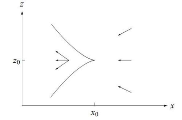
Figure 1: The curve with the cusp is the location of the fold caustic in the flow described by Eqs. (51). The arrows indicate local velocity vectors. There is one flow at every point to the right of the curve, and three flows at every point to its left.

giving the positions $(x,z)$ of particles in a flow from right to left with the particles on the right and top moving downwards and the particles on the right and bottom moving upwards. See Fig. 1. For simplicity, we take the flow to be stationary, and the acceleration to vanish everywhere. The particles are labeled by $(\alpha,\tau)$ where $\tau$ is an age parameter, defined as minus the time a particle crosses the $z=0$ axis. $\alpha$ labels the different trajectories. The velocities are

$$v_{z} = {\partial z\over\partial\tau}=b\alpha$$

$$v_{x} = {\partial x\over\partial\tau}=-c~{}~{}\ .$$ (52)

The density of the flow is

$$d(x,z)\equiv{d^{2}N\over dxdz}={d^{2}N\over d\alpha d\tau}{1\over|D(\alpha,\tau)|}$$ (53)

where

$$D(\alpha,\tau)=det\left({\partial(x,z)\over\partial(\alpha,\tau)}\right)=b(-s\alpha^{2}+c\tau)~{}~{}\ .$$ (54)

Caustics occur where $D(\alpha,\tau)=0$, i.e. where the map is singular. The equation $D(\alpha,\tau)=0$ defines the curve

$$x=x_{0}-{3\over 2}\left({sc^{2}\over b^{2}}\right)^{1\over 3}|z-z_{0}|^{2\over 3}~{}~{}\ ,$$ (55)

shown by the solid line in Fig. 1. There are three flows at every location to the left of the curve whereas there is only one flow in the region to its right. The number of flows at a location $(x,z)$ is the number of $(\alpha,\tau)$ values that solve Eqs. (51). The curve is the location of a fold caustic. The cusp caustic is the special point $(x_{0},z_{0})$. When the curve is traversed starting on the side with three flows, two of the flows disappear. At any point other than $(x_{0},z_{0})$, the density and the velocity dispersion of those two flows behave as described in the previous subsection, i.e. the density diverges as ${1\over\sqrt{h}}$ where $h$ is the distance to the curve and the dispersion in the velocity component perpendicular to the curve also diverges as ${1\over\sqrt{h}}$. The dispersion in the velocity component parallel to the curve remains finite.

In this subsection, we are interested in the behavior of the density and velocity dispersion at the cusp. A complete answer can be given by obtaining the inverse of the map in Eqs. (51). This involves solving a third order polynomial equation, and inserting the resulting functions $\alpha(x,z)$ and $\tau(x,z)$ into the RHS of Eqs. (54) and (53). Here we content ourselves with the behavior of the density and the velocity dispersion ellipse when the cusp is approached from particular directions. If the cusp is approached along the $z=z_{0}$ axis from the right ($x>x_{0}$), the single flow there has $\alpha=0$ and $\tau=-(x-x_{0})/c$. The density of that flow is

$$d(x,z_{0})={d^{2}N\over d\alpha d\tau}{1\over b|x-x_{0}|}~{}~{}\ .$$ (56)

If the cusp is approached along the $x=x_{0}$ axis, from the top or from the bottom, the single flow there has $\tau=-{s\over 2c}\alpha^{2}$ and $z-z_{0}=-{bs\over 2c}\alpha^{3}$. The density is

$$d(x_{0},z)={d^{2}N\over d\alpha d\tau}~{}{1\over 3}\left({2\over bsc^{2}}\right)^{1\over 3}{1\over|z-z_{0}|^{2\over 3}}~{}~{}\ .$$ (57)

If the cusp is approached along the $z=z_{0}$ axis from the left ($x<x_{0}$) there are three flows: i) $\alpha=0$ and $\tau=(x_{0}-x)/c$, ii) $\tau=0$ and $\alpha=\sqrt{{2\over s}(x_{0}-x)}$, and iii) $\tau=0$ and $\alpha=-\sqrt{{2\over s}(x_{0}-x)}$. Flow i) has the same density as given in Eq. (56) whereas flows ii) and iii) each have half the density given in Eq. (56).

To obtain the velocity dispersions we consider a set of maps, as in Eq. (51), but with a distribution ${d^{5}N\over dz_{0}~{}db~{}dx_{0}~{}dc~{}ds}$ of the constants $z_{0}$, $b$, $x_{0}$, $c$ and $s$ that appear there. We assume that the distribution is narrowly peaked around average values of these constants. We consider small deviations $dz_{0}$ … $ds$ of the constants from their average values plus small deviations $d\alpha$ and $d\tau$ in the flow parameters such that

$$dz = dz_{0}+db\alpha\tau+bd\alpha\tau+b\alpha d\tau=0$$

$$dx = dx_{0}-dc\tau-cd\tau-{1\over 2}ds\alpha^{2}-s\alpha d\alpha=0~{}~{}\ .$$ (58)

Eqs. (58) imply that, at a given physical point, the deviations in the flow parameters are given in terms of the deviations in the constants by

$$\left(\begin{array}[]{cc}b\tau{}{}&~{}~{}b\alpha\\ s\alpha{}{}&~{}~{}c\end{array}\right)\left(\begin{array}[]{c}d\alpha\\ d\tau\end{array}\right)=\left(\begin{array}[]{c}-dz_{0}-\alpha\tau db\\ dx_{0}-\tau dc-{1\over 2}\alpha^{2}ds\end{array}\right)~{}~{}\ .$$ (59)

When approaching the cusp, $\alpha\rightarrow 0$ and $\tau\rightarrow 0$, the RHS of Eq. (59) goes to $\left({-dz_{0}\atop dx_{0}}\right)$, and therefore

$$\left(\begin{array}[]{c}d\alpha\\ d\tau\end{array}\right)={1\over b(c\tau-s\alpha^{2})}\left(\begin{array}[]{cc}c{}{}&~{}~{}-b\alpha\\ -s\alpha{}{}&~{}~{}b\tau\end{array}\right)\left(\begin{array}[]{c}-dz_{0}\\ dx_{0}\end{array}\right)~{}~{}\ .$$ (60)

Likewise, when approaching the cusp, the deviations in the velocity components are

$$dv_{z} = bd\alpha=-{cdz_{0}\over c\tau-s\alpha^{2}}$$

$$dv_{x} = -dc~{}~{}\ .$$ (61)

Hence

$$\delta v_{z}=\sqrt{<(dv_{z})^{2}>}={c\delta z_{0}\over|c\tau-s\alpha^{2}|}~{}~{}~{},~{}~{}~{}\delta v_{x}=\delta c~{}~{}\ .$$ (62)

If $dz_{0}$ and $dc$ are correlated

$$<dv_{z}~{}dv_{x}>={c\over c\tau-s\alpha^{2}}<dz_{0}~{}dc>~{}~{}\ .$$ (63)

For each of the flows at the cusp, the dispersion in the velocity component parallel to the axis ($\hat{x}$) of the cusp remains finite whereas the dispersion in the component of velocity in the direction perpendicular ($\hat{z}$) to the axis of the cusp diverges. This might have been expected since the flow folds in the direction perpendicular to the axis of the cusp. The phase space densiy remains finite since the divergence of the physical density is canceled by the divergence of the velocity dispersion.

V Applications to the Big Flow

In the Caustic Ring Model of the Milky Way halo, the dark matter density on Earth is dominated by a single cold flow, dubbed the ‘Big Flow’, because of our proximity to a cusp in the 5th caustic ring in our galaxy. In the Caustic Ring Model, there are two flows on Earth associated with the 5th caustic ring. Their velocity vectors are MWcr MWhalo

$$\vec{v}_{5\pm}\simeq(505~{}\hat{\phi}\pm 120~{}\hat{r})~{}{\rm km/s}$$ (64)

where $\hat{\phi}$ is the unit vector in the direction of Galactic rotation and $\hat{r}$ the unit vector in the radially outward direction. The density of the Big Flow on Earth is estimated to be $1.5\cdot 10^{-24}$ gr/cm³. The density of the other flow associated with the 5th caustic ring, hereafter called the ‘Little Flow’, is estimated to be $0.15\cdot 10^{-24}$ gr/cm³. It is not known whether the Big Flow has velocity $\vec{v}_{5-}$ and the Little Flow has velocity $\vec{v}_{5+}$, or vice-versa. The existence of the Big Flow provides strong additional motivation for high resolution analysis of the output of a cavity detector of dark matter axions, since it produces a prominent narrow peak in the energy spectrum. The width of the peak determines the signal to noise ratio of a high resolution search for it. The width of the peak is the energy dispersion of the Big Flow. Here we place an upper limit on the energy dispersion of the Big Flow from the observed sharpness of the 5th caustic ring. The same upper limit applies to the Little Flow.

The best lower limit on the sharpness of the 5th caustic ring is obtained by considering a triangular feature in the Infrared Astronomical Sattelite (IRAS) map of the Galactic plane MWcr . The feature is in a direction tangent to the 5th caustic ring. The gravitational fields of caustic rings of dark matter leave imprints upon the spatial distribution of ordinary matter. Looking tangentially to a caustic ring, from a vantage point in the plane of the ring, one may have the good fortune of recognizing the tricusp shape sing of the cross-section of a caustic ring. The IRAS map of the Galactic plane in the direction tangent to the 5th caustic ring shows such a feature. The relevant IRAS maps are posted at http://www.phys.ufl.edu/ sikivie/triangle. The triangular feature is correctly oriented with respect to the galactic plane and the galactic center. Its position is consistent within measurement errors with the position of the sharp rise in the Galactic rotation curve due to the 5th caustic ring. If the velocity dispersion of the flow forming the 5th caustic ring were large, the triangular feature in the IRAS map would be blurred. The sharpness of the triangular feature in the IRAS map implies that the 5th caustic ring is spread over a distance less than approximately 10 pc.

V.1 Upper limit on the Big Flow energy dispersion

The particles forming a caustic ring fall in and out of the galaxy near the galactic plane. Let $E$ and $L$ be respectively the energy and angular momentum of the particles that form the 5th caustic ring and are in the galactic plane. We have

$$E={1\over 2}v_{r}(r)^{2}+{L^{2}\over 2r^{2}}+V(r)$$ (65)

where $v_{r}(r)$ is the radial velocity of the particles at galactocentric radius $r$ and $V(r)$ is the gravitational potential in which they move. We will use

$$V(r)=v_{\rm rot}^{2}\ln(r)$$ (66)

consistent with a flat galactic rotation curve, with rotation velocity $v_{\rm rot}$. For the Milky Way, $v_{\rm rot}\simeq$ 220 km/s. The inner radius $a$ of a caustic ring is the distance of closest approach to the galactic center of the particles in the galactic plane. Therefore

$$E={L^{2}\over 2a^{2}}+V(a)~{}~{}\ .$$ (67)

Small deviations $dE$, $dL$ and $da$ from the average values of $E$, $L$ and $a$ are related by

$$dE={LdL\over a^{2}}-{L^{2}\over a^{3}}da+{dV\over dr}(a)da~{}~{}\ .$$ (68)

In view of Eq. (66) this may be rewritten

$$da={a\over v_{\rm rot}^{2}-v_{\phi}(a)^{2}}(dE-{LdL\over a^{2}})$$ (69)

where $v_{\phi}(r)=L/r$ is the velocity in the direction of galactic rotation of the particles that are in the galactic plane. The spread $\delta a$ in caustic ring radius is therefore given by

$$(\delta a)^{2}\equiv<(da)^{2}>={a^{2}\over(v_{\rm rot}^{2}-v_{\phi}(a)^{2})^{2}}[(\delta E)^{2}+{L^{2}\over a^{4}}(\delta L)^{2}-2{L\over a^{2}}<dE~{}dL>]$$ (70)

where, as in Section III, brackets indicate averaging over the ${d^{2}N\over dEdL}$ distribution of the dark matter particles, $\delta E\equiv\sqrt{<(dE)^{2}>}$ and $\delta L\equiv\sqrt{<(dL)^{2}>}$. The second term in the square brackets on the RHS of Eq. (70) dominates over the first term since

$${a^{2}\delta E\over L\delta L}={av_{\rm av}\over v_{\phi}(a)D_{\rm av}}$$ (71)

and $v_{\rm av}$ is of order $v_{\phi}(a)$ whereas $D_{\rm av}$ is much larger than $a$, as was discussed in Section III. The second term also dominates over the third term since

$$<dE~{}dL>~{}\sim~{}\delta E~{}\delta L~{}{a\over R}~{}<<~{}\delta E~{}\delta L~{}~{}\ .$$ (72)

Hence

$$\delta a\simeq\sigma_{v}{v_{\phi}(a)D_{\rm av}\over v_{\phi}^{2}(a)-v_{\rm rot}^{2}}\simeq{\sigma_{v}\over 426~{}{\rm km/s}}D_{\rm av}$$ (73)

where we used $v_{\phi}(a)=520$ km/s MWhalo . It remains to estimate $D_{\rm av}$, the average distance from the galactic center where the processes took place by which the flow presently constituting the 5th caustic ring acquired velocity dispersion. Of course it is hard to give a precise value. The present turnaround radius of the flow constituting the 5th caustic ring is $R_{5}$ = 121 kpc MWhalo . As a rough estimate, we set $D_{\rm av}\sim R_{5}/2$. With $\delta a\lesssim$ 10 pc, this yields

$$\sigma_{v}\lesssim 71~{}{\rm m/s}~{}~{}\ .$$ (74)

In ref. MWcr , an upper limit on $\sigma_{v}$ was estimated using $\delta a\sim{R\over v}\sigma_{v}$ with $R$ the turnaround radius and $v$ the velocity of the flow at the caustic. This yielded $\sigma_{v}\lesssim 53$ m/s. Although far more work went into justifying Eqs. (73) and (74), the two estimates are qualitatively consistent since $D_{\rm av}\sim R$ and $v=v_{\phi}(a)$. The difference between the two estimates may be taken as a measure of the uncertainty on the bound. At any rate, the bound on $\sigma_{v}$ from the sharpness of caustic rings is extraordinarily severe in view of the commonly made assertion that the dark matter falling onto a galaxy is in clumps with velocity dispersion of order 10 km/s.

To obtain an upper limit on the energy dispersion $~{}\delta E=mv_{\rm av}\sigma_{v}$ of the flow forming the 5th caustic ring we set $v_{\rm av}\sim$ 300 km/s. This yields

$${\delta E\over m}\lesssim 2.4\cdot 10^{-10}~{}~{}\ .$$ (75)

If the axion frequency is 1 GHz, as in the example given in the Introduction, the upper limit on the widths of the peaks associated with the Big Flow and the Little Flow in the cavity detector of dark matter axions is of order 0.24 Hz. Let us emphasize that there is nothing to suggest that the upper bound is saturated.

V.2 Velocity dispersion ellipse of the Big Flow

In the Caustic Ring Model of the Milky Way halo, the Big Flow has a large density on Earth as a result of our proximity to a cusp in the 5th caustic ring of dark matter. The inner radius of the 5th caustic ring, derived from a rise in the Milky Way rotation curve and from the triangular feature in the IRAS map of the Galactic plane, is $a$ = 8.31 kpc whereas its outer radius is $a+p$ = 8.44 kpc MWcr . See Fig. 2. These values assume that our own distance to the Galactic center, which sets the scale, is 8.5 kpc. Note that the values of the inner and outer radii are at the tangent point of our line of sight to the 5th caustic ring. If axial symmetry is assumed, as in the Caustic Ring Model, we are just outside the tricusp cross-section of the 5th caustic ring, near the cusp at the outer radius, which we call henceforth the ‘outer cusp’. In that case there are two flows on Earth associated with the 5th caustic ring, the Big Flow and the Little Flow. The uncertainty on the density of the Big Flow is large since it is sensitive to our distance to the outer cusp. Axial symmetry need not be a good approximation in this context. It could be sufficiently broken that we are located inside the tricusp instead of just outside. If we are located inside the tricusp, there are four flows on Earth associated with the 5th caustic ring. If we are inside the tricusp and near the outer cusp three of the flows are Big Flows and the fourth is the Little Flow. The Little Flow is the same as before. It does not participate in the outer cusp singularity. The Big Flows do participate in the outer cusp singularity. The densities, velocities and velocity dispersions of the Big Flows are given by the equations in Section IV as a function of position relative to the cusp. The Big Flows all have comparatively large dispersions in the component of velocity perpendicular to the symmetry axis of the cusp, i.e. their velocity ellipses are elongated in the direction perpendicular to the Galactic plane.

VI Summary

Motivated by the prospect that dark matter may some day be detected on Earth, we set out to predict properties of the velocity dispersion ellipsoid of the Big Flow. The Big Flow dominates the local dark matter distribution in the Caustic Ring Model of the Milky Way halo due to our proximity to the 5th caustic ring of dark matter in our galaxy. We analyzed a cold collisionless stationary flow in one dimension and derived how the velocity dispersion changes along such a flow. In one dimension the problem is simple because energy conservation and Liouville’s theorem control the outcome. To make headway in two dimensions we assumed that the potential in which the particles fall is axially symmetric as well as time-independent so that both energy and angular momentum are conserved. We derive the evolution of the velocity dispersion ellipse along a stationary axially symmetric flow under those assumptions. The local velocity dispersion always becomes large when approaching a caustic because the density becomes large but the phase space density is constant. We introduced a technique for obtaining the leading behavior of the velocity dispersion near caustics, and applied the technique to fold and cusp caustics. Finally we used our results to obtain an upper limit on the energy dispersion of the Big Flow from the observed sharpness of the 5th caustic ring and a prediction for the dispersion in its velocity components.

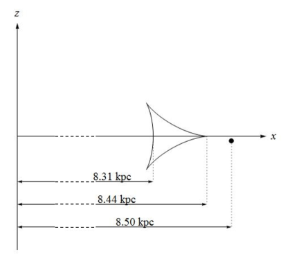
Figure 2: Relative position of the Sun and the 5th caustic ring in the Caustic Ring Model of the Milky Way halo. The Sun’s position is indicated by the dot. The $x$-axis is parallel to the Galactic plane. The tricusp shape is the cross-section of the 5th caustic ring. The model assumes axial symmetry. Because of axial symmetry breaking, the size of the tricusp and the position of the Sun relative to it may differ from what the figure shows.

- (1) Reviews include: Particle Dark Matter edited by Gianfranco Bertone, Cambridge University Press 2010; E.W. Kolb and M. Turner, The Early Universe, Addison Wesley 1990.
- (2) P.A.R. Ade et al. (the Planck Collaboration), arXiv:1303.5076.
- (3) L. Baudis, Dark matter searches, Annalen Phys. (2015).
- (4) P. Sikivie, Phys. Rev. Lett. 51 (1983) 1415.
- (5) S. DePanfilis et al., Phys. Rev. Lett. 59 (1987) 839; C. Hagmann et al., Phys. Rev. D42 (1990) 1297; C. Hagmann et al., Phys. Rev. Lett. 80 (1998) 2043; S.J. Asztalos et al., Phys. Rev. Lett. 104(2010) 041301.
- (6) L.D. Duffy et al., Phys. Rev. Lett. 95 (2005) 091304; L.D. Duffy et al., Phys. Rev. D74 (2006) 012006.
- (7) P. Sikivie and J. Ipser, Phys. Lett. B291 (1992) 288.
- (8) P. Sikivie, Phys. Lett. B432 (1998) 139.
- (9) P. Sikivie, Phys. Rev. D60 (1999) 063501.
- (10) A. Natarajan and P. Sikivie, Phys. Rev. D73 (2006) 023510.
- (11) A. Natarajan and P. Sikivie, Phys. Rev. D72 (2005) 083513.
- (12) F.-S. Ling, P. Sikivie and S. Wick, Phys. Rev. D70 (2004) 123503.
- (13) J.A. Fillmore and P. Goldreich, Ap. J. 281 (1984) 1; E. Bertschinger, Ap. J. Suppl. 58 (1985) 39.
- (14) P. Sikivie, I. Tkachev and Y. Wang, Phys. Rev. Lett. 75 (1995) 2911 and Phys. Rev. D 56 (1997) 1863.
- (15) L. Duffy and P. Sikivie, Phys. Rev. D78 (2008) 063508.
- (16) P. Sikivie, Phys. Lett. B567 (2003) 1.
- (17) H. Newberg et al., Ap. J. 569 (2002) 245; S.R. Majewski et al., Ap.J. 599 (2003) 1082.
- (18) J. Peebles, Principles of Physical Cosmology, Princeton University Press 1993.