ACDC: A Structured Efficient Linear Layer

Abstract

The linear layer is one of the most pervasive modules in deep learning representations. However, it requires $O(N^{2})$ parameters and $O(N^{2})$ operations. These costs can be prohibitive in mobile applications or prevent scaling in many domains. Here, we introduce a deep, differentiable, fully-connected neural network module composed of diagonal matrices of parameters, $\mathbf{A}$ and $\mathbf{D}$, and the discrete cosine transform $\mathbf{C}$. The core module, structured as $\mathbf{A}\mathbf{C}\mathbf{D}\mathbf{C}^{-1}$, has $O(N)$ parameters and incurs $O(N\log N)$ operations. We present theoretical results showing how deep cascades of $\operatorname{ACDC}$ layers approximate linear layers. $\operatorname{ACDC}$ is, however, a stand-alone module and can be used in combination with any other types of module. In our experiments, we show that it can indeed be successfully interleaved with ReLU modules in convolutional neural networks for image recognition. Our experiments also study critical factors in the training of these structured modules, including initialization and depth. Finally, this paper also points out avenues for implementing the complex version of $\operatorname{ACDC}$ using photonic devices.

1 Introduction

The linear layer is the central building block of nearly all modern neural network models. A notable exception to this is the convolutional layer, which has been extremely successful in computer vision; however, even convolutional networks typically feed into one or more linear layers after processing by convolutions. Other specialized network modules including LSTMs (Hochreiter & Schmidhuber, 1997), GRUs (Cho et al., 2014), the attentional mechanisms used for image captioning (Xu et al., 2015) and machine translation (Bahdanau et al., 2015), reading in Memory Networks (Sukhbaatar et al., 2015), and both reading and writing in Neural Turing Machines (Graves et al., 2015), are all built from compositions of linear layers and nonlinear modules, such as sigmoid, softmax and ReLU layers.

The linear layer is essentially a matrix-vector operation, where the input $\mathbf{x}$ is scaled with a matrix of parameters $\mathbf{W}$ as follows:

$$\mathbf{y}=\mathbf{x}\mathbf{W}$$ (1)

When the number of inputs and outputs is $N$, the number of parameters stored in $\mathbf{W}$ is $O(N^{2})$. It also takes $O(N^{2})$ operations to compute the output $\mathbf{y}$.

In spite of the ubiquity and convenience of linear layers, their $O(N^{2})$ size is extremely wasteful. Indeed, several studies focusing on feedforward perceptrons and convolutional networks have shown that the parametrisation of linear layers is extremely wasteful, with up to 95% of the parameters being redundant (Denil et al., 2013; Gong et al., 2014; Sainath et al., 2013).

Given the importance of this research topic, we have witnessed a recent explosion of works introducing structured efficient linear layers (SELLs). We adopt the following notation to describe SELLs within a common framework:

$$\mathbf{y}=\mathbf{x}\boldsymbol{\Phi}=\mathbf{x}\boldsymbol{\Phi}(\mathbf{D},\mathbf{P},\mathbf{S},\mathbf{B})$$ (2)

We reserve the capital bold symbol $\mathbf{D}$ for diagonal matrices, $\mathbf{P}$ for permutations, $\mathbf{S}$ for sparse matrices, and $\mathbf{B}\in\{\mathbf{F},\mathbf{H},\mathbf{C}\}$ for bases such as Fourier, Hadamard and Cosine transforms respectively. In this setup, the parameters are typically in the diagonal or sparse entries of the matrices $\mathbf{D}$ and $\mathbf{S}$. Sparse matrices aside, the computational cost of most SELLs is $O(N\log N)$, while the number of parameters is reduced from $O(N^{2})$ to a mere $O(N)$. These costs are a consequence of the facts that we only need to store the diagonal matrices, and that the Fourier, Hadamard or Discrete Cosine transforms can be efficiently computed in $O(N\log N)$ steps.

Often the diagonal and sparse matrices have fixed random entries. When this is the case, we will use tildes to indicate this fact (e.g., $\tilde{\mathbf{D}}$).

Our first SELL example is the Fast Random Projections method of Ailon & Chazelle (2009):

$$\boldsymbol{\Phi}=\tilde{\mathbf{D}}\mathbf{H}\tilde{\mathbf{S}}$$ (3)

Here, the sparse matrix $\tilde{\mathbf{S}}$ has Gaussian entries, the diagonal $\tilde{\mathbf{D}}$ has $\{+1,-1\}$ entries drawn independently with probability $1/2$, and $\mathbf{H}$ is the Hadamard matrix. The embeddings generated by this SELL preserve metric information with high probability, as formalized by the theory of random projections.

Fastfood (Le et al., 2013), our second SELL example, extends fast random projections as follows:

$$\boldsymbol{\Phi}=\tilde{\mathbf{D}}_{1}\mathbf{H}\mathbf{P}\tilde{\mathbf{D}}_{2}\mathbf{H}\tilde{\mathbf{D}}_{3}.$$ (4)

In (Yang et al., 2015), the authors introduce an adaptive variant of Fastfood, with the random diagonal matrices replaced by diagonal matrices of parameters, and show that it outperforms the random counterpart when applied to the problem of replacing one of the fully connected layers of a convolutional neural network for ImageNet (Jia et al., 2014). Interestingly, while the random variant is competitive in simple applications (MNIST), the adaptive variant has a considerable advantage in more demanding applications (ImageNet).

The adaptive SELLs, including Adaptive Fastfood and the alternatives discussed subsequently, are end to end differentiable. They require only $O(N)$ parameters and $O(N\log N)$ operations in both the forward and backward passes of backpropagation. These benefits can be achieved both at train and test time.

Cheng et al. (2015) introduced a SELL consisting of the product of a circulant matrix ($\mathbf{R}$) and a random diagonal matrix ($\tilde{\mathbf{D}}_{1}$). Since circulant matrices can be diagonalized with the discrete Fourier transform (Golub & Van Loan, 1996), this SELL falls within our general notation:

$$\boldsymbol{\Phi}=\tilde{\mathbf{D}}_{1}\mathbf{R}=\tilde{\mathbf{D}}_{1}\mathbf{F}\mathbf{D}_{2}\mathbf{F}^{-1}.$$ (5)

Sindhwani et al. (2015) introduced a Toeplitz-like structured transform, within the framework of displacement operators. Since Toeplitz matrices can be “embedded” in circulant matrices, they can also be diagonalized with the discrete Fourier transform (Golub & Van Loan, 1996).

In this work, we introduce a SELL that could be thought of as an adaptive variant of the method of Cheng et al. (2015). In addition, instead of using a (single) shallow SELL as in previous works (Yang et al., 2015; Cheng et al., 2015; Sindhwani et al., 2015), we consider deep SELLs:

$$\boldsymbol{\Phi}=\prod_{k=1}^{K}\mathbf{A}_{k}\mathbf{F}\mathbf{D}_{k}\mathbf{F}^{-1}.$$ (6)

Here, $\mathbf{A}$ is also a diagonal matrix of parameters, but we use a different symbol to emphasize that $\mathbf{A}$ scales the signal in the original domain while $\mathbf{D}$ scales it in the Fourier domain.

While adaptive SELLs perform better than their random counterparts in practice, there is a lack of theory for adaptive SELLs. Moreover, the empirical studies of recent adaptive SELLs have many deficiencies. For instance, it is often not clear how performance varies depending on implementation, and many critical details such as initialization and the treatment of biases are typically obviated. In addition, the gains are often demonstrated in models of different size, making objective comparison very difficult.

In addition to demonstrating good performance replacing the fully connected layers of CaffeNet, we present a theoretical approximation guarantee for our deep SELL in Section 3. We also discuss the crucial issue of implementing deep SELLs efficiently in modern GPU architectures in Section 5 and release this software with this paper. This engineering contribution is important as many of the recently proposed methods for accelerating linear layers often fail to take into account the attributes and limitations of GPUs, and hence fail to be adopted.

1.1 Lightning fast deep SELL

Figure 1: Example of a $4f$ system. This system implements the multiplication of an optical signal by a circulant matrix $\mathbf{F}\mathbf{D}\mathbf{F}^{-1}$. The lenses apply Fourier transforms to the signal and the diffraction element applies the diagonal multiplication.

Our deep SELL (equation (6)) offers several possibilities for analog physical implementation. Given the great demand for fast low energy neural networks, the possibility of harnessing physical phenomena to perform efficient computation in deep networks is worthy of consideration.

In the Fourier optics field, it is well known that the two-dimensional Fourier transform can be implemented with a paraxial optical system consiting of a lens of focal length $f$ in free space. In this setup, known as a $2f$ system, a waveform in the frontal focal plane of the lens, viewed as a two-dimensional complex array, is transformed to another one in the focal plane behind the lens that corresponds to the Fourier transform of the array. A $4f$ system is obtained by placing a diffractive element in between two $2f$ systems at a distance $f$ from each (shown in Figure 1).

Every circulant matrix $\mathbf{R}=\mathbf{F}\mathbf{D}\mathbf{F}^{-1}$ can be realized optically using a $4f$ system, with the transformation by the diffractive optical device corresponding to the multiplication by the complex diagonal matrix $\mathbf{D}$ (Reif & Tyagi, 1997; Müller-Quade et al., 1998; Huhtanen, 2008; Schmid et al., 2000). Moreover, paraxial diffractive optical systems with consecutive products of circulant and diagonal matrices can factor a complex matrix into products of diagonal and circulant matrices (Müller-Quade et al., 1998; Huhtanen & Perämäki, 2015). Hence, in principle the mapping of equation (6) can be implemented with optical elements.

In a separate research community, Hermans & Vaerenbergh (2015) recently discussed using waves in a trainable medium for learning linear layers by backpropagation, and suggested a potential implementation using an integrated photonics chip. The nanophotonic chip consists of a cascade of unitary trasformations of the optical signals interleaved with tuneable waveguides (phase shifters). Hermans & Vaerenbergh (2015) present an abstraction of this chip. In particular, if we let $\mathbf{o}$ and $\mathbf{o}^{\prime}$ represent the optical fields at the input and output waveguides, the chip implements the following transformation:

$$\mathbf{o}^{\prime}=\prod_{k=1}^{K}\mathbf{D}_{k}\mathbf{U}_{k}\mathbf{o}$$ (7)

where $\mathbf{U}_{k}$ is a unitary transformation of the signal and $\mathbf{D}_{k}$ is a diagonal matrix $\mathbf{D}_{k}=\mathrm{diag}(\exp(j\boldsymbol{\varphi}_{k}))$ with tuneable phase shifts $\boldsymbol{\varphi}_{k}$. By restricting the diagonal matrices in equation (6) to be of this complex form, the circulant $\mathbf{R}=\mathbf{F}\mathbf{D}\mathbf{F}^{-1}$ is unitary and we obtain an equivalence between equations (6) and (7). This points to a potential nanophotonic implementation of our complex deep SELL.

More recently, Saade et al. (2015) disclosed an invention that peforms optical analog random projections.

2 Further related works

The literature on this topic is vast, and consequently this section only aims to capture some of the significant trends. We refer readers to the related work sections of the papers cited in the previous and present section for further details.

As mentioned earlier, many studies have shown that the parametrisation of linear layers is extremely wasteful (Denil et al., 2013; Gong et al., 2014; Sainath et al., 2013). In spite of this redundancy, there has been little success in improving the linear layer, since natural extensions, such as low rank factorizations, lead to poor performance when trained end to end. For instance, Sainath et al. (2013) demonstrate significant improvements in reducing the number of parameters of the output softmax layers, but only modest improvements for the hidden linear layers.

Several methods based on low-rank decomposition and sparseness have been proposed to eliminate parameter redundancy at test time, but they provide only a partial solution as the full network must be instantiated during training (Collins & Kohli, 2014; Xue et al., 2013; Blundell et al., 2015; Liu et al., 2015; Han et al., 2015b). That is, these approaches require training the original full model. Hashing techniques have been proposed to reduce the number of parameters (Chen et al., 2015; Bakhtiary et al., 2015). Hashes have irregular memory access patterns and, consequently, good performance on large GPU-based platforms is an open problem. Distillation (Hinton et al., 2015; Romero et al., 2015) also offers a way of compressing neural networks, as a post-processing step.

Novikov et al. (2015) use a multi-linear transform (Tensor-Train decomposition) to attain significant reductions in the number of parameters in some of the linear layers of convolutional networks.

3 Deep SELL

We define a single component of deep SELL as $\operatorname{AFDF}(\mathbf{x})=\mathbf{x}\mathbf{A}\mathbf{F}\mathbf{D}\mathbf{F}^{-1}$, where $\mathbf{F}$ is the Fourier transform and $\mathbf{A},\mathbf{D}$ are complex diagonal matrices. It is straightforward to see that the AFDF transform is not sufficient to express an arbitrary linear operator $\mathbf{W}\in\mathbb{C}^{n\times n}$. An AFDF transform has $2n$ degrees of freedom, whereas an arbitrary linear operator has $n^{2}$ degrees of freedom.

To this end, we turn our attention to studying compositions of AFDF transforms. By composing AFDF transforms we can boost the number of degrees of freedom, and we might expect that any linear operator could be constructed as a composition of sufficiently many AFDF transforms. In the following we show that this is indeed possible, and that a bounded number of AFDF transforms is sufficient.

Definition 1.

The order-$K$ AFDF transformation is the composition of $K$ consecutive AFDF operations with (optionally) different $\mathbf{A}$ and $\mathbf{D}$ matrices. We write an order-$K$ complex AFDF transformation as follows

$$\mathbf{y}=\operatorname{AFDF}_{K}(\mathbf{x})=\mathbf{x}\left[\prod_{k=1}^{K}\mathbf{A}_{k}\mathbf{F}\mathbf{D}_{k}\mathbf{F}^{-1}\right].$$ (8)

We also assume, without loss of generality, that $\mathbf{A}_{1}=\mathbf{I}$ so that $\operatorname{AFDF}_{1}(\mathbf{x})=\mathbf{x}\mathbf{F}\mathbf{D}_{1}\mathbf{F}^{-1}$.

For the analysis it will be convenient to rewrite the AFDF transformation in a different way, which we refer to as the optical presentation.

Definition 2.

If $\mathbf{y}=\operatorname{AFDF}_{K}(\mathbf{x})$ then we define the optical presentation of an order-$K$ AFDF transform as

$$\hat{\mathbf{y}}=\hat{\mathbf{x}}\left[\prod_{k=1}^{K-1}\mathbf{D}_{k}\mathbf{R}_{k+1}\right]\mathbf{D}_{K}$$

where $\hat{\mathbf{x}}$ and $\hat{\mathbf{y}}$ are the Fourier transforms of $\mathbf{x}$ and $\mathbf{y}$, and $\mathbf{R}_{k+1}=\mathbf{F}^{-1}\mathbf{A}_{k+1}\mathbf{F}$.

Remark 3.

The matrix $\mathbf{R}=\mathbf{F}^{-1}\mathbf{A}\mathbf{F}$ is circulant. This follows from the duality between convolution in the spatial domain and pointwise multiplication in the Fourier domain.

The optical presentation shows how the spectrum of $\mathbf{x}$ is related to the spectrum of $\mathbf{y}$. Importantly, it shows that we can express an order-$K$ AFDF transform as a linear operator in Fourier space that is composed of a product of circulant and diagonal matrices. Transformations of this type are well studied in the Fourier optics literature, as they can be realized with cascades of lenses.

Of particular relevance to us is the main result of Huhtanen & Perämäki (2015) which states that almost all (in the Lebesgue sense) matrices $\mathbf{M}\in\mathbb{C}^{N\times N}$ can be factored as

$$\mathbf{M} =\left[\prod_{i=1}^{N-1}\mathbf{D}_{2i-1}\mathbf{R}_{2i}\right]\mathbf{D}_{2N-1}$$

where $\mathbf{D}_{2j-1}$ is diagonal and $\mathbf{R}_{2j}$ is circulant. This factorization corresponds exactly to the optical presentation of an order-$N$ AFDF transform, therefore we conclude the following:

Theorem 4.

An order-$N$ AFDF transform is sufficient to approximate any linear operator in $\mathbb{C}^{N\times N}$ to arbitrary precision.

Proof.

Every AFDF transform has an optical presentation, and by the main result of Huhtanen & Perämäki (2015) operators of this type are dense in $\mathbb{C}^{N\times N}$. ∎

4 ACDC: A practical deep SELL

Thus far we have focused on a complex SELL, where theoretical guarantees can be obtained. In practice we find it useful to consider instead a real SELL. The real version of $\operatorname{AFDF}_{K}$, denoted $\operatorname{ACDC}_{K}$ has the same form as Equation (8), with complex diagonals replaced with real diagonals, and Fourier transforms replaced with Cosine Transforms. This change departs from the theory of Section 3; however, our experiments show that this does not appear to be a problem in practice.

The reasons for considering ACDC over AFDF are purely practical.

1. Most existing deep learning frameworks support only real numbers, and thus working with real valued transformations simplifies the interface between our SELL and the rest of the network.

2. Working with complex numbers effectively doubles the memory footprint of of the transform itself, and more importantly, of the activations that interact with it.

The importance of the second point should not be underestimated, since the computational complexity of our SELL is quite low, a typical GPU implementation will be bottlenecked by the overhead of moving data through the GPU memory hierarchy. Reducing the amount of data to be moved allows for a significantly faster implementation. We discuss these concerns in more detail in Section 5.

In this work, we use the DCT (type II) matrix with entries

$$c_{nk}=\sqrt{\frac{2}{N}}\left[\epsilon_{k}\cos\left(\frac{\pi(2n+1)k}{2N}\right)\right]$$ (9)

for $n,k=0,1,\ldots,N$, and where $\epsilon_{k}=1/\sqrt{2}$ for $k=0$ or $k=N$ and $\epsilon_{k}=1$ otherwise. DCT matrices are real and orthogonal: $\mathbf{C}^{-1}=\mathbf{C}^{T}$. Moreover, the DCTs are separable transforms. That is, the DCT of a multi-dimensional signal can be decomposed in terms of successive DCTs of the appropriate one-dimensional components of the signal. The DCT can be computed efficiently using the Fast Fourier Transform (FFT) algorithm (or the specialized fast cosine transform).

Denoting $\mathbf{h}_{1}=\mathbf{x}_{i}\mathbf{A}$, $\mathbf{h}_{2}=\mathbf{h}_{1}\mathbf{C}$, $\mathbf{h}_{3}=\mathbf{h}_{2}\mathbf{D}$, $\mathbf{y}_{i}=\mathbf{h}_{3}\mathbf{C}^{-1}$, and $\mathbf{A}=\operatorname{diag}(\mathbf{a}),\mathbf{D}=\operatorname{diag}(\mathbf{d})$ we have the following derivatives in the backward pass:

$$\frac{\partial{L}}{\partial{\mathbf{d}}}=\frac{\partial{\mathbf{y}_{i}}}{\partial{\mathbf{d}}}\frac{\partial{L}}{\partial{\mathbf{y}_{i}}}=\frac{\partial{\mathbf{h}_{2}\mathbf{D}}}{\partial{\mathbf{d}}}\frac{\partial{\mathbf{h}_{3}\mathbf{C}^{-1}}}{\partial{\mathbf{h}_{3}}}\frac{\partial{L}}{\partial{\mathbf{y}_{i}}}=\operatorname{diag}(\mathbf{h}_{2})\mathbf{C}\frac{\partial{L}}{\partial{\mathbf{y}_{i}}}=\mathbf{h}_{2}\odot\mathbf{C}\frac{\partial{L}}{\partial{\mathbf{y}_{i}}}$$ (10)

$$\frac{\partial{L}}{\partial{\mathbf{D}}}=\operatorname{diag}(\frac{\partial{L}}{\partial{\mathbf{d}}})$$ (11)

$$\frac{\partial{L}}{\partial{\mathbf{a}}}=\frac{\partial{\mathbf{y}_{i}}}{\partial{\mathbf{a}}}\frac{\partial{L}}{\partial{\mathbf{y}_{i}}}=\frac{\partial{\mathbf{x}_{i}\mathbf{A}}}{\partial{\mathbf{a}}}\frac{\partial{\mathbf{h}_{1}\mathbf{C}}}{\partial{\mathbf{h}_{1}}}\frac{\partial{\mathbf{h}_{2}\mathbf{D}}}{\partial{\mathbf{h}_{2}}}\frac{\partial{L}}{\partial{\mathbf{h}_{3}}}=\mathbf{x}_{i}\odot\mathbf{C}^{-1}\mathbf{d}\odot\mathbf{C}\frac{\partial{L}}{\partial{\mathbf{y}_{i}}}$$ (12)

$$\frac{\partial{L}}{\partial{\mathbf{A}}}=\operatorname{diag}(\frac{\partial{L}}{\partial{\mathbf{a}}})$$ (13)

$$\frac{\partial{L}}{\partial{\mathbf{x}_{i}}}=\frac{\partial{\mathbf{y}_{i}}}{\partial{\mathbf{x}_{i}}}\frac{\partial{L}}{\partial{\mathbf{y}_{i}}}=\frac{\partial{\mathbf{x}_{i}\mathbf{A}}}{\partial{\mathbf{x}_{i}}}\frac{\partial{L}}{\partial{\mathbf{h}_{1}}}=\mathbf{a}\odot\mathbf{C}^{-1}\mathbf{d}\odot\mathbf{C}\frac{\partial{L}}{\partial{\mathbf{y}_{i}}}$$ (14)

5 Efficient implementation of ACDC

The processor used to benchmark the ACDC layer was an NVIDIA Titan X. The peak floating point throughput of the Titan X is 6605 GFLOPs, and the peak memory bandwidth is 336.5GB/s. This gives an arithmetic intensity (FLOPs per byte) of approximately 20. In the ideal case, where there is enough parallelism for the GPU to hide all latencies, an algorithm with a higher arithmetic intensity than this would be expected to be floating point throughput bound, while an algorithm with lower arithmetic intensity would be expected to be memory throughput bound.

The forward pass of a single example through a size-$N$ ACDC layer when calculated using 32-bit floating point arithmetic requires at least $24N$ bytes to be moved to and from main memory. Eight bytes per element for each of $\mathbf{A}$ and $\mathbf{D}$, four bytes per element for the input, and four bytes per element for the output. It also requires approximately $4N+5N\log_{2}(N)$ floating point operations. When batching, the memory transfers for $\mathbf{A}$ and $\mathbf{D}$ are expected to be cached as they are reused for each example in the batch, so for the purposes of calculating arithmetic intensity in the batched case it is reasonable to discount them. The arithmetic intensity of a minibatch passing through an ACDC layer is therefore approximately:

$$AI=(4+5\log_{2}(N))/8$$

For the values of $N$ we are interested in ($128\longrightarrow 16,384$) this arithmetic intensity varies between 4.9 and 9.3, indicating that the peak performance of a large ACDC layer with a large batch size is expected to be limited by the peak memory throughput of the GPU (336.5GB/s), and that optimization of an ACDC implementation should concentrate on removing any extraneous memory operations.

Two versions of ACDC have been implemented. One performs the ACDC in a single call, with the minimum of $8N$ bytes moved per layer (assuming perfect caching of $\mathbf{A}$ and $\mathbf{D}$). The other performs ACDC with multiple calls, with significantly more than $8N$ bytes moved per layer.

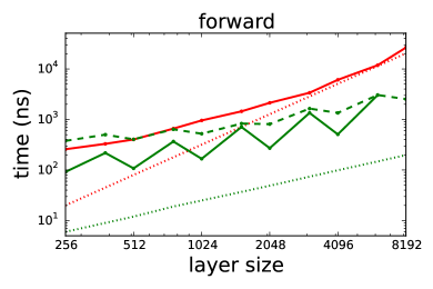
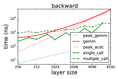
Figure 2: Performance comparison of theoretical and actual performance of our ACDC implementations to an ordinary dense linear layer using a batch size of 128. Peak curves show maximum theoretical performance achievable by the hardware.

5.1 Single call implementation

To minimize traffic to and from main memory intermediate loads or stores during the layer must be eliminated. To accomplish this kernel fusion is used to fuse all of the operations of ACDC into a single call, with intermediate values being stored in temporary low-level memory instead of main memory. This presents two challenges to the implementation.

Firstly, the size of the ACDC layer is limited by the availability of temporary memory on the GPU. This limits the size of the ACDC layer that can be calculated. It also has performance implications: the temporary memory used to store intermediate values in the computation is shared with the registers required for basic calculation, such as loop indices. The more of this space that is used by data, the fewer threads can fit on the GPU at once, limiting parallelism.

Secondly, the DCT and IDCT layers must be written by hand so that they can be efficiently fused with the linear layers. Implementations of DCT and IDCT are non-trivial, and a generic implementation able to handle any input size would be a large project in itself. For this reason, the implementation is constrained to power-of-two and multiples of large power-of-two layer sizes.

5.2 Multiple call implementation

While expected to be less efficient a multiple call implementation is both much simpler programmatically, and much more generically usable. Using the method of Makhoul (1980) it is possible to perform size-$N$ DCTs and IDCTs using size-$N$ FFTs. As such, the NVIDIA library cuFFT can be used to greatly simplify the code required, as well as achieve reasonable performance across a wide range of ACDC sizes. The procedure is as follows:

1. Multiply input by $\mathbf{A}$ and set up $\mathbf{C}_{1}$

2. Perform $\mathbf{C}_{1}$ using a C2C cuFFT call

3. Finalize $\mathbf{C}_{1}$, multiply by $\mathbf{D}$ and setup $\mathbf{C}_{2}$

4. Perform $\mathbf{C}_{2}$ using a C2C cuFFT call

5. Finalize $\mathbf{C}_{2}$

The total memory moved for this implementation is significantly higher as each call requires a load and a store for each element. The performance trade-off with the single call method is therefore one of parallelism against memory traffic.

5.3 Performance Comparison

Figure 2 compares the speed of the single and multiple call implementations of ACDC against dense matrix-matrix multiplication for a variety of layer sizes.

It is clear that in both the forward and backward pass ACDC layers have a significantly lower runtime than fully connected layers using dense matrices. Even if the matrix-matrix operations were running at peak, ACDC still would outperform them by up to 10 times.

As expected, the single call version of ACDC outperforms the multiple call version, although for smaller layer sizes the gap is larger. When the layer size increases the multiple call version suffers significantly more from small per-call overheads. Both single and multiple call versions of ACDC perform significantly worse on non power-of-two layer sizes. This is because they rely on FFT operations, which are known to be more efficient when the input sizes are of lengths $z^{n}$, where $z$ is a small integer.

While the backward pass of ACDC is expected to take approximately the same time as the forward pass, it takes noticeably longer. To compute the parameter gradients one needs the input into the $\mathbf{D}$ operation and the gradient of the output from the $\mathbf{A}$ operation. As the aim of the layer is to reduce memory footprint it was decided instead to recompute these during the backward pass, increasing runtime while saving memory.

6 Experiments

6.1 Linear layers

In this section we show that we are able to approximate linear operators using ACDC as predicted by the theory of Section 3. These experiments serve two purposes

1. They show that recovery of a dense linear operator by SGD is feasible in practice. The theory of Section 3 guarantees only that it is possible to approximate any operator, but does not provide guidance on how to find this approximation. Additionally, Huhtanen & Perämäki (2015) suggest that this is a difficult problem.

2. They validate empirically that our decision to focus on ACDC over the complex AFDF does not introduce obvious difficulties into the approximation. The theory provides guarantees only for the complex case, and the experiments in this section suggest that restricting ourselves to real matrices is not a problem.

We investigate using ACDC on a synthetic linear regression problem

$$\mathbf{Y}=\mathbf{X}\mathbf{W}_{true}+\boldsymbol{\epsilon},$$ (15)

where $\mathbf{X}$ of size $10,000\times 32$ and $\mathbf{W}_{true}$ of size $32\times 32$ are both constructed by sampling their entries uniformly at random in the unit interval. Gaussian noise $\boldsymbol{\epsilon}\sim\mathcal{N}(0,10^{-4})$ is added to the generated targets.

The results of approximating the operator $\mathbf{W}_{true}$ using $\operatorname{ACDC}_{K}$ for different values of $K$ are shown in Figure 3. The theory of Section 3 predicts that, in the complex case, for a $32\times 32$ matrix it should be sufficient to have 32 layers of ACDC to express an arbitrary $\mathbf{W}_{true}$.

We found that initialization of the matrices $\mathbf{A}$ and $\mathbf{D}$ to identity $\mathbf{I}$, with Gaussian noise $\mathcal{N}(0,10^{-2})$ added the diagonals in order to break symmetries, is essential for models having many ACDC layers. (We found the initialization to be robust to the specification of the noise added to the diagonals.)

The need for thoughtful initialization is very clear in Figure 3. With the right initialization (leftmost plot), the approximation results of Section 3 are confirmed, with improved accuracy as we increase the number of ACDC layers. However, if we use standard strategies for initializing linear layers (rightmost plot), we observe very poor optimization results as the number of ACDC layers increases.

This experiment suggests that fewer layers suffice to arrive at a reasonable approximation of the original $\mathbf{W}_{true}$ than what the theory guarantees. With neural networks in mind this is a very relevant observation. It is well known that the linear layers of neural networks are compressible, indicating that we do not need to express an arbitrary linear operator in order to achieve good performance. Instead, we need only express a sufficiently interesting subset of matrices, and the result with 16 ACDC layers points to this being the case.

In Section 6.2 we show that by interspersing nonlinearities between ACDC layers in a convolutional network it is possible to use dramatically fewer ACDC layers than the theory suggests are needed while still achieving good performance.

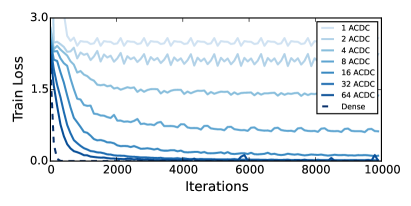
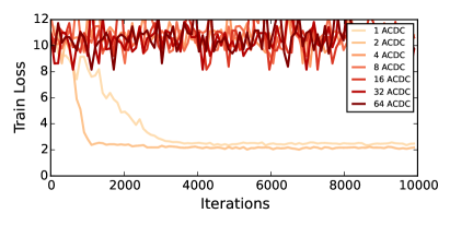
Figure 3: Training loss for different number of ACDC layers compared to loss for the dense matrix. Left: Initialization: $\mathcal{N}(1,\sigma^{2})$ with $\sigma=10^{-1}$. Right: Initialization: $\mathcal{N}(0,\sigma^{2})$ with $\sigma=10^{-3}$. Note the difference in scale on the y-axis.

6.2 Convolutional networks

In this section we investigate replacing the fully connected layers of a deep convolutional network with a cascade of ACDC layers. In particular we use the CaffeNet architecture for ImageNet (Deng et al., 2009). We target the two fully connected layers located between features extracted from the last convolutional layer and the final logistic regression layer, which we replace with $12$ stacked ACDC transforms interleaved with ReLU non-linearities and permutations. The permutations assure that adjacent SELLs are incoherent.

The model was trained using the SGD algorithm with learning rate $0.1$ multiplied by $0.1$ every $100{,}000$ iterations, momentum $0.65$ and weight decay $0.0005$. The output from the last convolutional layer was scaled by $0.1$, and the learning rates for each matrix $\mathbf{A}$ and $\mathbf{D}$ were multiplied by $24$ and $12$. All diagonal matrices were initialized from $\mathcal{N}(1,0.061)$ distribution. No weight decay was applied to $\mathbf{A}$ or $\mathbf{D}$. Additive biases were added to the matrices $\mathbf{D}$, but not to $\mathbf{A}$, as this sufficed to provide the ACDC layer with a bias terms just before the ReLU non-linearities. Biases were initialized to $0$. To prevent the model from overfitting dropout regularization was placed before each of the last 5 SELL layers with dropout probability equal to $0.1$.

The resulting model arrives at $43.26\%$ error which is only $0.67\%$ worse when compared to the reference model, so SELL confidently stays within $1\%$ of the performance of the original network. We report this result, as well as a comparison to several other works in Table 1.

Test Time Post-Processing	Top-1 Err Increase	# of Param	Reduction
Collins & Kohli (2014)	1.81%	15.2M	x4.0
Han et al. (2015b)	0.00%	6.7M	x9
Han et al. (2015a) (P+Q)	0.00%	$\sim$2.3M	x27
Train and Test Time Reduction
Cheng et al. (2015) (Circulant CNN 2)	0.40%	$>$ 16.3M	$<$ x3.8
∗Novikov et al. (2015) (TT4 FC FC)	0.30%	-	x3.9
∗Novikov et al. (2015) (TT4 TT4 FC)	1.30%	-	x7.4
Yang et al. (2015) (Finetuned SVD 1)	0.14%	46.6M	x1.3
Yang et al. (2015) (Finetuned SVD 2)	1.22%	23.4M	x2.0
Yang et al. (2015) (Adaptive Fastfood 16)	0.30%	16.4M	x3.6
ACDC	0.67%	9.7M	x6.0
CaffeNet Reference Model	0.00%	58.7M	x1.0

Table 1: Comparison of SELL with alternative factorization methods achieving marginal performance drop on the ImageNet dataset. Entries in italics incur an increase in top-1 error of $>$1.0%. Entries marked with a star use VGG16, which makes them not directly comparable to our own. Previous works have shown that it is typically possible to achieve $\sim 30\%$ greater compression factors on VGG16 than on AlexNet-style architectures (Han et al., 2015a; b).

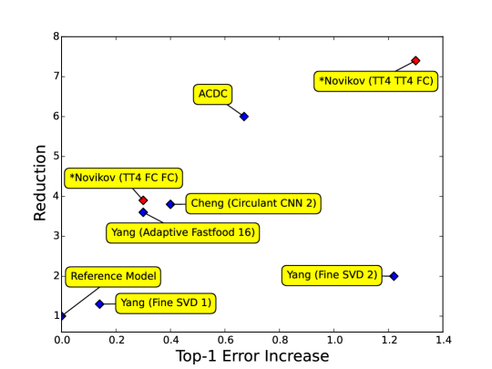
Figure 4: Visual comparison of the tradeoff between parameter and accuracy reduction for train time applicable SELLs. Red entries (marked with a star in the labels) use VGG16, which makes them not directly comparable to the others, as discussed in the caption of Table 1.

The two fully connected layers of CaffeNet, consisting of more than $41$ million parameters, are replaced with SELL modules which contain a combined $165,888$ parameters. These results agree with the hypothesis that neural networks are over-parameterized formulated by Denil et al. (2013) and supported by Yang et al. (2015). At the same time such a tremendous reduction without significant loss of accuracy suggests that SELL is a powerful concept and a way to use parameters efficiently.

This approach is an improvement over Deep Fried Convnets (Yang et al., 2015) and other FastFood (Le et al., 2013) based transforms in the sense that the layers remain narrow and become deep (potentially interleaved with non-linearites) as opposed to wide and shallow, while maintaining comparable or better performance. The result of narrower layers is that the final softmax classification layer requires substantially fewer parameters, meaning that the resulting compression ratio is higher.

Our experiment shows that ACDC transforms are an attractive building block for feedforward convolutional architectures, that can be used as a structured alternative to fully connected layers, while fitting very well into the deep learning philosophy of introducing transformations executed in steps as the signal is propagated down the network rather than projecting to higher-dimensional spaces.

It should be noted that the method of pruning proposed in (Han et al., 2015b) and the follow-up method of pruning, quantizing and Huffman coding proposed in (Han et al., 2015a) achieve compression rates between x9 and x27 on AlexNet by applying a pipeline of reducing operations on a trained models. Usually it is necessary to perform at least a few iterations of such reductions to arrive at the stated compression rates. For the AlexNet model one such iteration takes 173 hours according to (Han et al., 2015b). On top of that as this method requires training the original full model the time cost of that operation should be taken into consideration as well.

Compressing pipelines target models that are ready for deployment and function in the environment where amount of time spent on training is absolutely dominated by the time spent evaluating predictions. In contrast, SELL methods are appropriate for incorporation into the design of a model.

7 Conclusion

We introduced a new Structured Efficient Linear Layer, which adds to a growing literature on using memory efficient structured transforms as efficient replacements for the dense matrices in the fully connected layers of neural networks. The structure of our SELL is motivated by matrix approximation results from Fourier optics, but has been specialized for efficient implementation on NVIDIA GPUs.

We have shown that proper initialization of our SELL allows us to build very deep cascades of SELLs that can be optimized using SGD. Proper initialization is simple, but is essential for training cascades of SELLs with more than a few layers. Working with deep and narrow cascades of SELLs makes our networks more parameter efficient than previous works using shallow and wide cascades because the cost of layers interfacing between the SELL and the rest of the network is reduced (e.g. the size of the input to the dense logistic regression layer of the network is much smaller).

In future work we plan to investigate replacing the diagonal layers of ACDC with other efficient structured matrices such as band or block diagonals. These alternatives introduce additional parameters in each layer, but may give us the opportunity to explore the continuum between depth and expressive power per layer more precisely.

Another interesting avenue of investigation is to include SELL layers in other neural network models such as RNNs or LSTMs. Recurrent nets are a particularly attractive targets as they are typically composed entirely of linear layers. This means that the potential parameter savings are quite substantial, and since the computational bottleneck is in these models comes from matrix-matrix multiplications there is a potential speed advantage as well.

References

- Ailon & Chazelle (2009) Ailon, Nir and Chazelle, Bernard. The Fast Johnson Lindenstrauss Transform and approximate nearest neighbors. SIAM Journal on Computing, 39(1):302–322, 2009.
- Bahdanau et al. (2015) Bahdanau, Dzmitry, Cho, Kyunghyun, and Bengio, Yoshua. Neural machine translation by jointly learning to align and translate. In International Conference on Learning Representations, 2015.
- Bakhtiary et al. (2015) Bakhtiary, Amir H., Lapedriza, Àgata, and Masip, David. Speeding up neural networks for large scale classification using WTA hashing. arXiv preprint arXiv:1504.07488, 2015.
- Blundell et al. (2015) Blundell, Charles, Cornebise, Julien, Kavukcuoglu, Koray, and Wierstra, Daan. Weight uncertainty in neural networks. In ICML, 2015.
- Chen et al. (2015) Chen, Wenlin, Wilson, James T., Tyree, Stephen, Weinberger, Kilian Q., and Chen, Yixin. Compressing neural networks with the hashing trick. In ICML, 2015.
- Cheng et al. (2015) Cheng, Yu, Yu, Felix X, Feris, R, Kumar, Sanjiv, Choudhary, Alok, and Chang, Shih-Fu. An exploration of parameter redundancy in deep networks with circulant projections. In ICCV, 2015.
- Cho et al. (2014) Cho, Kyunghyun, Van Merriënboer, Bart, Gulcehre, Caglar, Bahdanau, Dzmitry, Bougares, Fethi, Schwenk, Holger, and Bengio, Yoshua. Learning phrase representations using rnn encoder-decoder for statistical machine translation. In Empiricial Methods in Natural Language Processing, 2014.
- Collins & Kohli (2014) Collins, Maxwell D. and Kohli, Pushmeet. Memory bounded deep convolutional networks. Technical report, University of Wisconsin-Madison, 2014.
- Deng et al. (2009) Deng, J., Dong, W., Socher, R., Li, L.-J., Li, K., and Fei-Fei, L. ImageNet: A Large-Scale Hierarchical Image Database. In CVPR, 2009.
- Denil et al. (2013) Denil, Misha, Shakibi, Babak, Dinh, Laurent, Ranzato, Marc’Aurelio, and de Freitas, Nando. Predicting parameters in deep learning. In NIPS, pp. 2148–2156, 2013.
- Golub & Van Loan (1996) Golub, Gene H. and Van Loan, Charles F. Matrix Computations. Johns Hopkins University Press, 1996.
- Gong et al. (2014) Gong, Yunchao, Liu, Liu, Yang, Ming, and Bourdev, Lubomir. Compressing deep convolutional networks using vector quantization. arXiv preprint arXiv:1412.6115, 2014.
- Graves et al. (2015) Graves, Alex, Wayne, Greg, and Danihelka, Ivo. Neural Turing machines. Technical report, Google DeepMind, 2015.
- Han et al. (2015a) Han, Song, Mao, Huizi, and Dally, William J. Deep compression: Compressing deep neural network with pruning, trained quantization and Huffman coding. arXiv preprint arXiv:1510.00149, 2015a.
- Han et al. (2015b) Han, Song, Pool, Jeff, Tran, John, and Dally, William J. Learning both weights and connections for efficient neural networks. In NIPS, 2015b.
- Hermans & Vaerenbergh (2015) Hermans, Michiel and Vaerenbergh, Thomas Van. Towards trainable media: Using waves for neural network-style training. arXiv preprint arXiv:1510.03776, 2015.
- Hinton et al. (2015) Hinton, Geoffrey E., Vinyals, Oriol, and Dean, Jeffrey. Distilling the knowledge in a neural network. arXiv preprint arXiv:1503.02531, 2015.
- Hochreiter & Schmidhuber (1997) Hochreiter, Sepp and Schmidhuber, Jürgen. Long short-term memory. Neural computation, 9(8):1735–1780, 1997.
- Huhtanen (2008) Huhtanen, Marko. Approximating ideal diffractive optical systems. Journal of Mathematical Analysis and Applications, 345:53–62, 2008.
- Huhtanen & Perämäki (2015) Huhtanen, Marko and Perämäki, Allan. Factoring matrices into the product of circulant and diagonal matrices. Journal of Fourier Analysis and Applications, 2015.
- Jia et al. (2014) Jia, Yangqing, Shelhamer, Evan, Donahue, Jeff, Karayev, Sergey, Long, Jonathan, Girshick, Ross, Guadarrama, Sergio, and Darrell, Trevor. Caffe: Convolutional architecture for fast feature embedding. arXiv preprint arXiv:1408.5093, 2014.
- Le et al. (2013) Le, Quoc, Sarlós, Tamás, and Smola, Alex. Fastfood – approximating kernel expansions in loglinear time. In ICML, 2013.
- Liu et al. (2015) Liu, Baoyuan, Wang, Min, Foroosh, Hassan, Tappen, Marshall, and Pensky, Marianna. Sparse convolutional neural networks. In CVPR, 2015.
- Makhoul (1980) Makhoul, John. A fast cosine transform in one and two dimensions. IEEE Transactions on Acoustics, Speech and Signal Processing, 28(1):27–34, 1980.
- Müller-Quade et al. (1998) Müller-Quade, Jörn, Aagedal, Harald, Beth, Th, and Schmid, Michael. Algorithmic design of diffractive optical systems for information processing. Physica D: Nonlinear Phenomena, 120(1):196–205, 1998.
- Novikov et al. (2015) Novikov, Alexander, Podoprikhin, Dmitry, Osokin, Anton, and Vetrov, Dmitry. Tensorizing neural networks. In NIPS, 2015.
- Reif & Tyagi (1997) Reif, John and Tyagi, Akhilesh. Efficient parallel algorithms for optical computing with the DFT primitive. Applied Optics, 36(29):7327–7340, 1997.
- Romero et al. (2015) Romero, Adriana, Ballas, Nicolas, Kahou, Samira Ebrahimi, Chassang, Antoine, Gatta, Carlo, and Bengio, Yoshua. FitNets: Hints for thin deep nets. In ICLR, 2015.
- Saade et al. (2015) Saade, Alaa, Caltagirone, Francesco, Carron, Igor, Daudet, Laurent, Dremeau, Angelique, Gigan, Sylvain, and Krzakala, Florent. Random projections through multiple optical scattering: Approximating kernels at the speed of light. arXiv preprint arXiv:1510.06664, 2015.
- Sainath et al. (2013) Sainath, Tara N., Kingsbury, Brian, Sindhwani, Vikas, Arisoy, Ebru, and Ramabhadran, Bhuvana. Low-rank matrix factorization for deep neural network training with high-dimensional output targets. In ICASSP, pp. 6655–6659, 2013.
- Schmid et al. (2000) Schmid, Michael, Steinwandt, Rainer, Müller-Quade, Jörn, Rötteler, Martin, and Beth, Thomas. Decomposing a matrix into circulant and diagonal factors. Linear Algebra and its Applications, 306(1–3):131–143, 2000.
- Sindhwani et al. (2015) Sindhwani, Vikas, Sainath, Tara N, and Kumar, Sanjiv. Structured transforms for small-footprint deep learning. In NIPS, 2015.
- Sukhbaatar et al. (2015) Sukhbaatar, Sainbayar, Szlam, Arthur, Weston, Jason, and Fergus, Rob. End-to-end memory networks. In NIPS, 2015.
- Xu et al. (2015) Xu, Kelvin, Ba, Jimmy, Kiros, Ryan, Cho, Kyunghyun, Courville, Aaron, Salakhutdinov, Ruslan, Zemel, Richard, and Bengio, Yoshua. Show, attend and tell: Neural image caption generation with visual attention. In ICML, 2015.
- Xue et al. (2013) Xue, Jian, Li, Jinyu, and Gong, Yifan. Restructuring of deep neural network acoustic models with singular value decomposition. In INTERSPEECH, pp. 2365–2369, 2013.
- Yang et al. (2015) Yang, Zichao, Moczulski, Marcin, Denil, Misha, de Freitas, Nando, Smola, Alex, Song, Le, and Wang, Ziyu. Deep fried convnets. In ICCV, 2015.