Charged gravastars in higher dimensions

Abstract

We explore possibility to find out a new model of gravastars in the extended $D$-dimensional Einstein-Maxwell spacetime. The class of solutions as obtained by Mazur and Mottola of a neutral gravastar [1, 2] have been observed as a compitent alternative to $D$-dimensional versions of the Schwarzschild-Tangherlini black hole. The outer region of the charged gravastar model therefore corresponds to a higher dimensional Reissner-Nordström black hole. In connection to this junction conditions, therefore we have formulated mass and the related Equation of State of the gravastar. It has been shown that the model satisfies all the requirements of the physical features. However, overall observational survey of the results also provide probable indication of non-applicability of higher dimensional approach for construction of a gravastar with or without charge from an ordinary $4$-dimensional seed as far as physical ground is concerned.

, , ,

1 Introduction

A decade or more ago Mazur and Mottola [1, 2] have proposed a new solution for the endpoint of a gravitationally collapsing neutral system. By extending the concept of Bose-Einstein condensation to gravitational systems they constructed a cold compact object which consists of an (i) interior de Sitter condensate phase, and (ii) exterior Schwarzschild geometry. These are separated by a phase boundary with a small but finite thickness $r_{2}-r_{1}=\delta$ of the thin shell, where $r_{1}$ and $r_{2}$ represent the interior and exterior radii of the gravastar. Therefore, the equation of state (EOS) under consideration are as follows:

I. Interior: $0\leq r<r_{1}$,  with EOS $p=-\rho$,

II. Shell: $r_{1}<r<r_{2}$,  with EOS $p=+\rho$,

III. Exterior: $r_{2}<r$,  with EOS $p=\rho=0.$

Here the presence of matter on the shell is required to achieve the stability of the systems under expansion by exerting an inward force to balance the repulsion from within. These types of gravitationally vacuum stars were termed as gravastars. Thereafter several scientists have been studied these models under different viewpoints and have opened up a new field of research as an alternative to Black Holes [3, 4, 5, 6, 7, 8, 9, 10, 11, 12, 13, 14, 15].

Very recently, a charged $(3+1)$-dimensional gravastar admitting conformal motion has proposed by some of our collaborators [16] in the framework of Mazur and Mottola model [1, 2]. In this work the authors provide an alternative to static black holes. However, energy density here is found to diverge in the interior region of the gravastar. This actually scales like an inverse second power of its radius and unfortunatelly makes the model singular at $r=0$. However, interestingly in one of the solutions it is shown that the total gravitational mass vanishes for vanishing charge and turns the total gravitational mass into an electromagnetic mass under certain conditions. An extention on charged gravastar of Usmani et al. [16] can be found in the work of Bhar [17] admitting conformal motion with higher dimensional space-time.

In the present study we generalize the four-dimensional work on gravastar by Usmani et al. [16] to the higher dimensional space-time, however without admitting conformal motion. Our main motivation here is to construct gravastars in the Einstein-Maxwell geometry and see the higher dimensional effects, if any. Therefore this investigation is also extension of the work of Bhar [17] without admitting conformal motion and that of Rahaman et al. [18] with charge where originally higher dimensional gravastar has been studied. A detailed discussion on higher dimension and its applications in various fields of astrophysics as well as cosmology has been provided in Ref. [18].

The plan of the present investigation is as follows: In Sec. 2 the Einstein-Maxwell space-time geometry has been provided as the background of the study whereas in Sec. 3 we discuss the Interior space-time, Exterior space-time and Thin shell cases of the gravastars with their respective solutions. The related junction conditions are provided in Sec. 4. We explore physical features of the models, viz. proper length, energy condition, entropy, mass and equation of state in Sec. 5. At the end in Sec. 6 we provide some critically discussed concluding remarks.

2 The Einstein-Maxwell space-time geometry

For higher dimensional gravastar, we assume a $D$-dimensional spacetime with the typical mathematical structure $R^{1}XS^{1}XS^{d}~{}(d=D-2)$, where $S^{1}$ is the range of the radial coordinate $r$ and $R^{1}$ is the time axis. Let us therefore consider a static spherically symmetric metric in $D=d+2$ dimension as

$$ds^{2}=-e^{\nu}dt^{2}+e^{\lambda}dr^{2}+r^{2}d\Omega_{d}^{2},$$ (1)

where $d\Omega_{d}^{2}$ is a linear element on a $d$-dimensional unit sphere, parametrized by the angles $\phi_{1},\phi_{2},...,\phi_{d}$, as follows: $d\Omega_{d}^{2}=d\phi_{d}^{2}+\sin_{2}\phi_{d}[d\phi_{d-1}^{2}+\sin_{2}\phi_{d-1}\{d\phi_{d-2}^{2}+...+\sin_{2}\phi_{3}(d\phi_{2}^{2}+\sin_{2}\phi_{2}d\phi_{1}^{2})...\}]$.

Now, the Hilbert action coupled to matter and electromagnetic field can be provided as

$$I=\int d^{D}x\sqrt{-g}\left[\frac{R_{D}}{16\pi G_{D}}+({L}_{m}+{F}_{ik}{F}^{ik})\right],$$ (2)

where $L_{m}$ is the matter part of the Lagrangian and $F_{ij}$ is the electromagnetic field tensor which is related to the electromagnetic potentials through the relation $F_{ij}=A_{i,j}-A_{j,i}.$

In the above Eq. (2) the term $R_{D}$ is the curvature scalar in $D$-dimensional spacetime whereas $G_{D}$ is the $D$-dimensional Newtonian constant and $L_{m}$ is the Lagrangian for matter-energy distribution.

The Einstein-Maxwell field equations now can be written as

$$G^{D}_{ij}=-8\pi G_{D}[T_{ij}^{m}+T_{ij}^{em}],$$ (3)

where $G^{D}_{ij}$ is the Einstein tensor in $D$-dimensional spacetime, $T_{ij}^{m}$ and $T_{ij}^{em}$ are the matter-energy and electromagnetic tensors respectively.

We assume that the interior of the star is filled up with perfect fluid and therefore the matter-energy tensors can be considered in the following form

$$T_{ij}^{m}=(\rho+p)u_{i}u_{j}+pg_{ij},$$ (4)

where $\rho$ is the energy density, $p$ is the isotropic pressure and $u^{i}$ (with $u_{i}u^{i}=1$) is the $D$-velocity of the fluid under consideration.

On the other hand, the electromagnetic tensors can be provided as

$$T_{ij}^{em}=-\frac{1}{4\pi{G}_{D}}\left[F_{jk}F_{i}^{k}-\frac{1}{4}g_{ij}F_{kl}F^{kl}\right].$$ (5)

The corresponding Maxwell electromagnetic field equations are

$${[{(-g)}^{1/2}F^{ij}],}_{j}=4\pi J^{i}{(-g)}^{1/2},$$ (6)

$$F_{[ij,k]}=0,,$$ (7)

where $J^{i}$ is the current four-vector satisfying $J^{i}=\sigma u^{i}$, the parameter $\sigma$ being the charge density.

Hence the Einstein-Maxwell field equation (3), for the metric (1) along with the energy-momentum tensors, Eqs. (4) - (7), can be provided in the following explicit forms

$$-e^{-\lambda}\left[\frac{d(d-1)}{2r^{2}}-\frac{d\lambda^{\prime}}{2r}\right]+\frac{d(d-1)}{2r^{2}}=8\pi G_{D}~{}\rho+E^{2},$$ (8)

$$e^{-\lambda}\left[\frac{d(d-1)}{2r^{2}}+\frac{d\nu^{\prime}}{2r}\right]-\frac{d(d-1)}{2r^{2}}=8\pi G_{D}~{}p-E^{2},$$ (9)

$$\frac{e^{-\lambda}}{2}\left[\nu^{\prime\prime}-\frac{\lambda^{\prime}\nu^{\prime}}{2}+\frac{{\nu^{\prime}}^{2}}{2}-\frac{(d-1)(\lambda^{\prime}-\nu^{\prime})}{r}+~{}~{}~{}~{}~{}~{}~{}~{}~{}~{}~{}~{}~{}~{}~{}~{}~{}~{}~{}~{}~{}\right.$$

$$\left.\frac{(d-1)(d-2)}{r^{2}}\right]-\frac{(d-1)(d-2)}{2r^{2}}=8\pi G_{D}~{}p+E^{2},~{}~{}~{}~{}~{}~{}~{}~{}~{}~{}~{}~{}$$

(10)

where $E$ is the electric field. Here the symbol ‘$\prime$’ denotes differentiation with respect to the radial parameter $r$ and $c=1$ (in geometrical unit).

Therefore, the energy conservation equation in the $D$-dimensions is given by

$$\frac{1}{2}\left(\rho+p\right)\nu^{\prime}+p^{\prime}=\frac{1}{4\pi{G}_{D}r^{d}}(r^{d}E^{2})^{\prime},$$ (11)

with the electric field $E$ as follows

$$(r^{d}E)^{\prime}=\frac{2\pi^{\frac{d+1}{2}}}{\Gamma(\frac{d+1}{2})}r^{d}\sigma(r)e^{\lambda/2}.$$ (12)

In traditional sense, the term $\sigma e^{\lambda/2}$ appearing in the right hand side of Eq. (12), is known as the volume charge density. The assumption $\sigma e^{\lambda/2}=\sigma_{0}r^{m}$, can consistently be understood as the higher dimensional volume charge density being polynomial function of $r$ where the constant $\sigma_{0}$ is the central charge density.

Now from the above Eq. (12) by assuming $\sigma e^{\lambda/2}=\sigma_{0}r^{m}$, we obtain the explicit form of the electric field as given by

$$E=\frac{q}{r^{d}}=\frac{2\pi^{\frac{d+1}{2}}\sigma_{0}}{\Gamma(\frac{d+1}{2})}\frac{r^{m+1}}{(d+m+1)}=Ar^{m+1},$$ (13)

where $A=\frac{2\pi^{\frac{d+1}{2}}\sigma_{0}}{\Gamma(\frac{d+1}{2})(d+m+1)}$.

3 The gravastar models

3.1 Interior space-time

Following [1] we assume that the EOS for the interior region has the form

$$p=-\rho.$$ (14)

The above EOS is known in the literature as a ‘false vacuum’, ‘degenerate vacuum’, or ‘$\rho$-vacuum’ [19, 20, 21, 22] which represents a repulsive pressure, an agent responsible for the accelerating phase of the Universe, and is termed as the $\Lambda$-dark energy [23, 24, 25, 26, 27]. It is argued by [16] that a charged gravastar seems to be connected to the dark star [28, 29, 30].

The above EOS along with Eq. (11) readily provides

$$p=-\rho=k_{1}{r^{2(m+1)}}+k_{2}.$$ (15)

where $k_{1}=\frac{A^{2}(2m+d+2)}{4\pi{G}_{D}(2m+2)}$ and $k_{2}$ is an integration constant. However, if we put $r=0$ in Eq. (15), then it easily assigns the value of the integration constant $k_{2}=p_{c}=-\rho_{c}$. In general there is no sufficient argument to take pressure and density to be zero at the junction surface. Actually, in the thin shell limit the pressure and density are step functions at the junction surface [31]. However, for the sake of brevity and convenience, if one considers boundary condition on the spherical surface that at $r=R$ the pressure and density in Eq. (15) vanish, then it yields $k_{2}=-k_{1}R^{2(m+1)}=-\rho_{c}$, i.e. through $k_{1}$ now $k_{2}$ is also dependent on the charge density $\sigma_{0}$. This simply provides an expression for the central density, $\rho_{c}=k_{1}R^{2(m+1)}$ and thus in the present case we are treating with a spherical stellar system with a constant central density or equivalently pressure which is acting outwardly.

If one agrees with the above argument, then one can trust on the relation between $k_{1}$ and $k_{2}$, and also to the charge density $σ_{0}$ as a consequent. This, therefore, makes someone to speculate about the “electromagnetic mass model (EMM).” It is to be noted that the spherically symmetric system being static the magnetic counterpart will not act here at all and hence the matter stress tensor is not completely electromagnetic in origin rather the electric part is associated only. However, even in this case one can borrow the phrase “electromagnetic mass model (EMM)” because of the fact that Lorentz [32] himself termed it like that and we are in the present situation coining the phrase due to historical reasons only.

Using Eq. (15) in the field equation (8), we get the expression of the metric potential $\lambda$ given by

$$e^{-\lambda}=1-\frac{2A^{2}}{d(d+2m+3)}r^{2(m+2)}+\frac{16\pi G_{D}k_{1}}{d(d+2m+3)}r^{2(m+2)}~{}~{}~{}~{}~{}~{}~{}~{}~{}$$

$$+\frac{16\pi G_{D}k_{2}}{d(d+1)}r^{2}+k_{3}r^{1-d},$$ (16)

where $k_{3}$ is an integration constant. Since $d>2$ for dimension higher than four and the solution is regular at $r=0$, so one can demand for $k_{3}=0$. Thus, Eq. (16) essentially reduces to

$$e^{-\lambda}=1-\frac{2A^{2}}{d(d+2m+3)}r^{2(m+2)}+\frac{16\pi G_{D}k_{1}}{d(d+2m+3)}r^{2(m+2)}+\frac{16\pi G_{D}k_{2}}{d(d+1)}r^{2}.$$ (17)

Again, using Eqs. (8), (9) and (15) one may obtain the following unique relation

$$\ln k=\lambda+\nu,$$ (18)

where $k$ is an integration constant.

Thus we have the interior solutions for the metric potentials $\lambda$ and $\nu$ as follows

$$e^{\nu}=ke^{-\lambda}=k\left[1-\frac{2A^{2}}{d(d+2m+3)}r^{2(m+2)}+\frac{16\pi G_{D}k_{1}}{d(d+2m+3)}r^{2(m+2)}\right.~{}~{}~{}~{}~{}~{}~{}~{}~{}$$

$$\left.+\frac{16\pi G_{D}k_{2}}{d(d+1)}r^{2}\right],~{}~{}~{}~{}$$

(19)

The active gravitational mass $M(r)$ in higher dimensions, can be now calculated as

$$M(R)=\int_{0}^{{r_{1}=R}}~{}\left[\frac{2\pi^{\frac{d+1}{2}}}{\Gamma\left(\frac{d+1}{2}\right)}\right]r^{d}\left[\rho+\frac{E^{2}}{8\pi}\right]dr~{}~{}~{}~{}~{}~{}~{}~{}~{}~{}~{}~{}~{}$$

$$=\frac{2\pi^{\frac{d+1}{2}}}{\Gamma\left(\frac{d+1}{2}\right)}\left[\frac{A^{2}}{8\pi}\frac{R^{2m+d+3}}{2m+d+3}-\frac{k_{1}R^{2m+d+3}}{2m+d+3}-\frac{k_{2}R^{d+1}}{d+1}\right].$$ (20)

This is the usual gravitating mass for a $d$-dimensional sphere of radius $R$ and energy density $\rho$. The space-time metric here turns out to be free from any central singularity. Another interesting point one can easily observe that the density, pressure and mass (Eqs. (15) and (20)) do vanish and via the metric potentials (Eqs. (19)) space-time becomes flat for vanishing charge density $\sigma_{0}$. Therefore, the interior solutions provide electromagnetic mass (EMM) model  [32, 33, 34, 35, 36, 37, 38, 39, 40, 41, 42, 43, 44, 16, 45]. This result suggests that the interior de Sitter vacuum of a charged gravastar is essentially an electromagnetic mass that must generate the gravitational mass [16]. A detailed discussion on this EMM model can be obtained in Ref. [18].

3.2 Exterior space-time

The exterior region defined by $p=\rho=0$ in higher dimensions is nothing but a generalization of Reissner-Nordström solution. Therefore, following [46] the Reissner-Nordström metric can be obtained as

$$ds^{2}=-\left(1-\frac{\mu}{r^{d-1}}+\frac{q^{2}}{r^{2(d-1)}}\right)dt^{2}~{}~{}~{}~{}~{}~{}~{}~{}~{}~{}~{}~{}~{}~{}~{}~{}$$

$$+\left(1-\frac{\mu}{r^{d-1}}+\frac{q^{2}}{r^{2(d-1)}}\right)^{-1}dr^{2}+d\Omega_{d}^{2}.$$ (21)

Here $\mu=16\pi G_{D}M/\Omega_{d}$ is the constant of integration with $M$, the mass of the black hole and ${\Omega}_{d}$, the area of a unit $d$-sphere as ${\Omega}_{d}=2\pi^{(\frac{d+1}{2})}/\Gamma(\frac{d+1}{2})$.

3.3 Intermediate thin shell

Here we assume that the thin shell contains ultra-relativistic fluid of soft quanta and obeys the EOS

$$p=\rho.$$ (22)

This relation represents essentially a stiff fluid model as envisioned by [47] in connection to cold baryonic universe and have been considered by several authors for various situations in cosmology [48, 49] as well as in astrophysics [50, 51, 52].

It is difficult to obtain a general solution of the field equations in the non-vacuum region, i.e. within the shell. We try to find an analytic solution within the thin shell limit, $0<(e^{-\lambda}\equiv h)<<1$. As an advantage of it, we may set $h$ to be zero to the leading order. Under this approximation, the field Eqs. (8) - (10), with the above EOS, may be recast in the following form

$$\frac{h^{\prime}}{2r}=\frac{(d-1)}{r^{2}}-\frac{2E^{2}}{d},$$ (23)

$$\frac{\nu^{\prime}h^{\prime}}{4}+\frac{(d-1)h^{\prime}}{2r}=-\frac{(d-1)}{r^{2}}+2E^{2}.$$ (24)

Integration of Eq. (20) immediately yields

$$h=2(d-1)\ln r-\frac{2A^{2}r^{2(m+2)}}{d(m+2)}+c_{1},$$ (25)

where $c_{1}$ is an integration constant. The other metric potential can be found as

$$e^{\nu}=\frac{c_{2}}{r^{2(2d-1)}}\left(\frac{r^{2m+4}}{d(d-1)-2A^{2}r^{2m+4}}\right)^{\frac{d-1}{m+2}},$$ (26)

where $c_{2}$ is an integration constant.

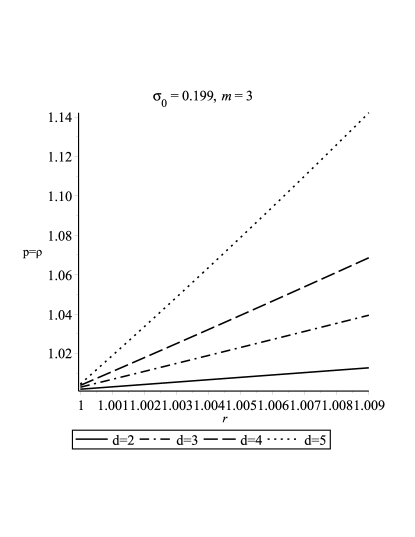
Figure 1: Variation of the pressure and density of the ultra relativistic matter in the shell against $r$ for different dimensions where the specific legends used are shown in the respective plots

Now in order to calculate the pressure as well as the matter density within the thin shell, using the Eq. (8) and the EOS Eq. (19), one may obtain

$$p=\rho=B\epsilon r^{2m+1}+c_{3}e^{-\nu},$$ (27)

where $B=\frac{A^{2}(2m+d+2)}{4\pi{G}_{D}}$ and $c_{3}$ is an integration constant. From Eq. (27) it can be observed that the pressure and matter density is depends on the central charge density and the thickness of the shell. The variation of the matter density over the shell is shown in Fig. 1 for different dimensions which shows that the matter density is increasing from the interior boundary to the exterior boundary.

4 Junction Condition

As mentioned earlier, in the gravastar configuration there are three regions: interior, shell and exterior region. Interior and exterior regions join at the junction interface of the shell. Though at the shell the metric coefficients are continuous but to see whether their derivatives are also continuous there we follow the Darmois-Israel condition [53, 54] to calculate the surface stresses at the junction interface. Therefore following the Lancozs equations for the intrinsic surface stress energy tensor $S_{ij}$, we can determine the surface energy density $(\Sigma)$ and surface pressure $p_{\theta_{1}}=p_{\theta_{2}}=...=p_{\theta_{d-1}}=p_{t}$ as

$$\Sigma=-\frac{d}{4\pi R}\left[\sqrt{1-\frac{\mu}{R^{d-1}}+\frac{q^{2}}{R^{2(d-1)}}}-~{}~{}~{}~{}~{}~{}~{}~{}~{}~{}~{}~{}~{}~{}~{}~{}~{}~{}~{}~{}~{}~{}~{}\right.$$

$$\left.\sqrt{1+\frac{16\pi G_{D}k_{1}R^{2(m+2)}}{d(d+2m+3)}-\frac{2A^{2}R^{2(m+2)}}{d(d+2m+3)}+\frac{16\pi G_{D}k_{2}R^{2}}{d(d+1)}}\right],$$ (28)

$$p_{t}=\frac{1}{8\pi R}\left[\frac{2(d-1)-\frac{(d-1)\mu}{R^{d-1}}}{\sqrt{1-\frac{\mu}{R^{d-1}}+\frac{q^{2}}{R^{2(d-1)}}}}-~{}~{}~{}~{}~{}~{}~{}~{}~{}~{}~{}~{}~{}~{}~{}~{}~{}~{}~{}~{}~{}~{}~{}~{}~{}~{}~{}~{}~{}~{}~{}~{}\right.$$

$$\left.\frac{{2(d-1)+\frac{32\pi G_{D}k_{1}(d+m+1)R^{2(m+2)}}{d(d+2m+3)}-\frac{4A^{2}(d+m+1)R^{2(m+2)}}{d(d+2m+3)}+\frac{32\pi G_{D}k_{2}R^{2}}{d+1}}}{\sqrt{1+\frac{16\pi G_{D}k_{1}R^{2(m+2)}}{d(d+2m+3)}-\frac{2A^{2}R^{2(m+2)}}{d(d+2m+3)}+\frac{16\pi G_{D}k_{2}R^{2}}{d(d+1)}}}\right].$$ (29)

5 Physical features of the models

5.1 Proper length

We consider that matter shell is situated at the surface $r=R$, describing the phase boundary of region I. The thickness of the shell ($\epsilon<<1$) is assumed to be very small. Thus the region III joins at the surface $r=R+\epsilon$.

Now, we calculate the proper thickness between two interfaces i.e. of the shell as

$$\ell=\int_{R}^{R+\epsilon}\sqrt{e^{\lambda}}dr=\int_{R}^{R+\epsilon}\frac{dr}{\sqrt{[c_{1}+2(d-1)\ln r-\frac{2A^{2}r^{2(m+2)}}{d(m+2)}]}}=\int_{R}^{R+\epsilon}\frac{dr}{f(r)}.$$ (30)

where $f(r)=\sqrt{[c_{1}+2(d-1)\ln r-\frac{2A^{2}r^{2(m+2)}}{d(m+2)}]}$.

To solve the above equation, let us consider that $\frac{df(r)}{dr}=\frac{1}{f(r)}$, so that we get

$$\ell=[f(R+\epsilon)-f(R)]\approx\epsilon\frac{df}{dr}\approx\frac{\epsilon}{\sqrt{[c_{1}+2(d-1)\ln r-\frac{2A^{2}r^{2(m+2)}}{d(m+2)}]}}.$$ (31)

As the value of $\epsilon$ is very small so the higher order terms of $\epsilon$ can be neglected. The variation of proper length for different dimensions with polynomial index is shown in Fig. 2.

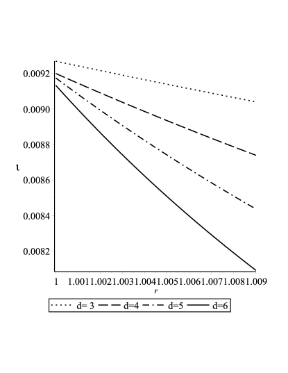
Figure 2: Variation of the length against $r$ for different dimensions where the specific legends used are shown in the respective plots

5.2 Energy

The energy $E$ within the shell can be calculated as

$$E=\int_{R}^{R+\epsilon}\left[\frac{2\pi^{\frac{d+1}{2}}}{\Gamma\left(\frac{d+1}{2}\right)}\right]r^{d}\left[\rho+\frac{E^{2}}{8\pi}\right]dr\approx\left[\frac{2\pi^{\frac{d+1}{2}}}{\Gamma\left(\frac{d+1}{2}\right)}\right]\left[\frac{\epsilon A^{2}}{8\pi}R^{2(m+1)+d}\right].$$ (32)

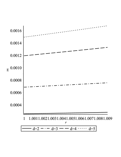
Figure 3: Variation of energy with $r$ for different dimensions where the specific legends used are shown in the respective plots

We have considered the energy ${E}$ within the shell up to the first order in $\epsilon$. The thickness $\epsilon$ of the shell being very small ($\epsilon<<1$), we expand it binomially about $R$ and consider first order of $\epsilon$ only. It can be observed that the energy within the shell (i) is proportional to $\epsilon$ in first order of thickness, and (ii) depends on the dimension $d$ of the spacetime. Fig. 3 shows energy profile of charged gravastar in higher dimension.

5.3 Entropy

Following Mazur and Mottola prescription [1] the entropy can be given as

$$S=\int_{R}^{R+\epsilon}\left[\frac{2\pi^{\frac{d+1}{2}}}{\Gamma\left(\frac{d+1}{2}\right)}\right]r^{d}s(r)\sqrt{e^{\lambda}}dr,$$ (33)

where $s(r)$ stands for the entropy density of the local temperature $T(r)$, which is written as

$$s(r)=\frac{\xi^{2}k_{B}^{2}T(r)}{4\pi\hbar^{2}}=\xi\left(\frac{k_{B}}{\hbar}\right)\sqrt{\frac{p}{2\pi}},$$ (34)

where $\xi$ is a dimensionless constant.

Now the entropy of the fluid within the shell can be given by

$$S\approx\left[\frac{2\pi^{\frac{d+1}{2}}}{\Gamma\left(\frac{d+1}{2}\right)}\right]\frac{\xi k_{B}\epsilon r^{d}}{\hbar\sqrt{2\pi}}\sqrt{\frac{B\epsilon r^{2m+1}+c_{3}e^{-\nu}}{c_{1}+2(d-1)lnr-\frac{2A^{2}r^{2(m+2)}}{d(m+2)}}}.$$ (35)

Following Ref. [16] it can be shown that (i) the thickness of the shell is negligibly small compared to its position from the center of the gravastar (i.e., if $\epsilon<<R$), and (ii) the entropy depends on the thickness of the shell.

5.4 Mass

Now, it is easy to find the surface mass $m_{s}$ of the thin shell from the equation

$$m_{s}=\frac{2\pi^{\frac{d+1}{2}}}{\Gamma(\frac{d+1}{2})}R^{d}\Sigma=\frac{2\pi^{\frac{d+1}{2}}}{\Gamma(\frac{d+1}{2})}\frac{dR^{d-1}}{4\pi}\Bigg{[}X-\sqrt{1-\frac{\mu}{R^{d-1}}+\frac{q^{2}}{R^{2(d-1)}}}\Bigg{]},$$ (36)

where $X=\sqrt{1+\frac{16\pi G_{D}k_{1}R^{2(m+2)}}{d(d+2m+3)}-\frac{2A^{2}R^{2(m+2)}}{d(d+2m+3)}+\frac{16\pi G_{D}k_{2}R^{2}}{d(d+1)}}.$

Using Eq. (36) we can determine the total mass of the gravastar in terms of the mass of the thin shell as

$$\mu=\frac{q^{2}}{R^{d-1}}-\left[\frac{16\pi G_{D}k_{1}R^{2m+d+3}}{d(d+2m+3)}-\frac{2A^{2}R^{2m+d+3}}{d(d+2m+3)}+\frac{16\pi G_{D}k_{2}R^{d+1}}{d(d+1)}\right.$$

$$\left.+\frac{m_{s}^{2}}{F^{2}R^{d-1}}-\frac{2m_{s}}{F}X\right],$$

(37)

where $F=\frac{2\pi^{\frac{d+1}{2}}}{\Gamma(\frac{d+1}{2})}\left[\frac{d}{4\pi}\right]$.

5.5 Equation of State

Let us assume $p_{\theta_{1}}=p_{\theta_{2}}=p_{\theta_{3}}=...=p_{t}=-\mathcal{P}$, here $\mathcal{P}$ is the surface tension as acts on the fluid of the gravastar.

Then Eqs. (28) and (29) yield

$$\mathcal{P}=\omega(R)\Sigma.$$ (38)

Thus the Equation of State parameter $\omega$ can be found as

$$\omega(R)=\frac{-1}{2d}\left[\frac{\frac{2(d-1)-(d-1)\frac{\mu}{R^{d-1}}}{\sqrt{1-\frac{\mu}{R^{d-1}}+\frac{q^{2}}{R^{2(d-1)}}}}+\frac{Y}{X}}{\sqrt{1-\frac{\mu}{R^{d-1}}+\frac{q^{2}}{R^{2(d-1)}}}-X}\right],$$ (39)

where $Y={2(d-1)+\frac{32\pi G_{D}k_{1}(d+m+1)R^{2(m+2)}}{d(d+2m+3)}-\frac{4A^{2}(d+m+1)R^{2(m+2)}}{d(d+2m+3)}+\frac{32\pi G_{D}k_{2}R^{2}}{d+1}}$.

6 Discussions and Conclusions

In the present study we have explored some possibilities to find out a new model of gravastars in contrast to the Mazur-Mottola type model of four-dimensional and neutral gravastar [1, 2], specifically seeking its generalization to: (i) the extended $D$-dimensional spacetime, and (ii) the Einstein-Maxwell geometry. Under these two considerations we have found out a class of solutions and hence some interesting results which can be observed as an alternative to $D$-dimensional versions of the Reissner-Nordström-Tangherlini black hole.

Some of the key physical features of the model are as follows:

(i) We have found out all the physical parameters e.g. metric potentials, thickness of the thin shell, energy, entropy etc. and our result matches to the result of [16] for $d=2$ and $m=0$ i.e. for $4$-dimensional space-time without any polynomial index. All the plots (Figs. 1 - 3) related to these parameters also suggest validity of physical requirements.

(ii) It is interesting to note that all the solutions are regular at the center $r=0$ and positive inside the interior region of the gravastar. Specifically, if we put $r=0$ in Eq. (15) then via the integration constant $k_{2}=p_{c}=-\rho_{c}$ we get a spherical system with a constant central density or pressure which being incompressible makes the gravastar free from singularity as well as stable.

(iii) We observe (from Eqs. (15) and (20)) that the density, pressure and mass like all the physical parameters do vanish and also the space-time becomes flat for vanishing charge density $\sigma_{0}$. Therefore, the interior solutions provides electromagnetic mass (EMM) model  [32, 33, 34, 35, 36, 37, 38, 39, 40, 41, 42, 43, 44, 16, 45]. This result suggests that unlike the work of Usmani et al. [16] and Rahaman et al. [45] the interior de Sitter vacuum of a charged gravastar is always an electromagnetic mass which must generate the gravitational mass rather in the present case a constant central pressure acts as repulsive force which prevents the system to undergo the fatal singularity .

As a final comment, we would like to put an important note here regarding overall observational results of the present investigation on gravastar with higher dimensional space-time. As a sample study a comparison between Figs. 1 - 3 shows that there are lots of quantitative change in the profiles of the physical parameters and as one goes on towards higher dimentions much appreciable results can be observed. All these observational surveys are probable indication of applicability of higher dimensional approach for construction of a gravastar with or without charge from an ordinary $4$-dimensional seed. In connection to this concluding remark we note that in the work of Bhar et al. [55], where they have performed an investigation on the possibility of higher dimensional compact stars, the results are in favour of our present study.

References

- [1] P. Mazur, E. Mottola, arXiv:gr-qc/0109035, Report number: LA-UR-01-5067 (2001).
- [2] P. Mazur, E. Mottola, Proc. Natl. Acad. Sci. USA 101 (2004) 9545 .
- [3] M. Visser et al., Class. Quant. Gravit. 21 (2004) 1135 .
- [4] C. Cattoen, T. Faber, M. Visser, Class. Quant. Gravit. 22 (2005) 4189 .
- [5] B.M.N. Carter, Class. Quant. Gravit. 22 (2005) 4551.
- [6] N. Bilic et al., JCAP 0602 (2006) 013 .
- [7] F. Lobo, Class. Quant. Gravit. 23 (2006) 1525.
- [8] A. DeBenedictis et al., Class. Quant. Gravit. 23 (2006) 2303.
- [9] F. Lobo et al., Class. Quant. Gravit. 24 (2007) 1069.
- [10] D. Horvat et al., Class. Quant. Gravit. 24 (2007) 4191.
- [11] B.M.H. Cecilia et al., Class. Quant. Gravit. 24 (2007) 5637.
- [12] P. Rocha et al., J. Cosmol. Astropart. Phys. 11 (2008) 010.
- [13] D. Horvat, S. Ilijic and A. Marunovic, Class. Quant. Gravit. 26 (2009) 025003.
- [14] K.K. Nandi et al., Phys. Rev. D 79 (2009) 024011.
- [15] B.V. Turimov, B.J. Ahmedov, A.A. Abdujabbarov, Mod. Phys. Lett. A 24 (2009) 733.
- [16] A.A. Usmani, F. Rahaman, S. Ray, K.K. Nandi, P.K.F. Kuhfittig, Sk.A. Rakib, Z. Hasan, Phys. Lett. B 701 (2011) 388.
- [17] P. Bhar, Astrophys. Space Sci., 354 (2014) 457.
- [18] F. Rahaman, S. Chakraborty, S. Ray, A.A. Usmani, S. Islam, Int. J. Theor. Phys. 54 (2015) 50.
- [19] P.C.W. Davies, Phys. Rev. D 30 (1984) 737.
- [20] J.J. Blome, W Priester, Naturwis. 71 (1984) 528.
- [21] C. Hogan, Nat. 310 (1984) 365.
- [22] N. Kaiser, A. Stebbins, Nat. 310 (1984) 391.
- [23] A.G. Riess et al., Astron. J. 116 (1998) 1009.
- [24] S. Perlmutter et al., Astrophys. J. 517 (1999) 565.
- [25] S. Ray, U. Mukhopadhyay, X.-H. Meng, Gravit. Cosmol. 13 (2007) 142.
- [26] A.A. Usmani, P.P. Ghosh, U. Mukhopadhyay, P.C. Ray, S. Ray, Mon. Not. R. Astron. Soc. 386 (2008) L92.
- [27] J. Frieman, M. Turner, D. Huterer, Ann. Rev. Astron. Astrophys. 46 (2008) 385.
- [28] F.S.N. Lobo, gr-qc/0805.2309.
- [29] R. Chan, M.F.A. da Silva, J.F.V. da Rocha, Gen. Relativ. Gravit. 41 (2009a) 1835.
- [30] R. Chan, M.F.A. da Silva, J.F.V. da Rocha, Mod. Phys. Lett. A 24 (2009b) 1137.
- [31] P.O. Mazur, E. Mottola, Class. Quant. Grav. 32 (2015) 215024.
- [32] H.A. Lorentz, Proc. Acad. Sci., Amsterdam 6 (1904) (Reprinted in The Principle of Relativity, Dover, INC., p. 24,1952).
- [33] J.A. Wheeler, Geometrodynamics, Academic, New York, p. 25 (1962).
- [34] R.P. Feynman, R.R. Leighton, M. Sands, The Feynman Lectures on Physics, Addison-Wesley, Palo Alto, Vol. II, Chap. 28 (1964).
- [35] F. Wilczek, Phys. Today 52 (1999) 11.
- [36] P.S. Florides, Proc. Camb. Phil. Soc. 58 (1962) 102.
- [37] F.I. Cooperstock, V. de la Cruz, Gen. Relativ. Gravit. 9 (1978) 835.
- [38] R.N. Tiwari, J.R. Rao, R.R. Kanakamedala, Phys. Rev. D 30 (1984) 489.
- [39] R. Gautreau, Phys. Rev. D 31 (1985) 1860.
- [40] Ø. Grøn, Phys. Rev. D 31 (1985) 2129.
- [41] J. Ponce de Leon, J. Math. Phys. 28 (1987) 410.
- [42] S. Ray, B. Das, Mon. Not. Roy. Astron. Soc. 349 (2004) 1331.
- [43] S. Ray, Int. J. Mod. Phys. D 15 (2006) 917.
- [44] S. Ray et al., Ind. J. Phys. 82 (2008) 1191.
- [45] F. Rahaman, A.A. Usmani, S. Ray, S. Islam, Phys. Lett. B 717 (2015) 1.
- [46] F.R. Tangherlini, Nuo. Cim. 27 (1963) 636.
- [47] Y.B. Zel’dovich, Mon. Not. R. Astron. Soc. 160 (1972) 1P.
- [48] B.J. Carr, Astrophys. J. 201 (1975) 1.
- [49] M.S. Madsen, J.P. Mimoso, J.A. Butcher, G.F.R. Ellis, Phys. Rev. D 46 (1992) 1399.
- [50] T. Buchert, Gen. Relativ. Gravit. 33 (2001) 1381.
- [51] T.M. Braje, R.W. Romani, Astrophys. J. 580 (2002) 1043.
- [52] L.P. Linares, M. Malheiro, S. Ray, Int. J. Mod. Phys. D 13 (2004) 1355.
- [53] G. Darmois, Memorial des sciences mathematiques XXV, Fasticule XXV ch V (Gauthier-Villars, Paris, France, 1927)
- [54] W. Israel, Nuo. Cim. B 44, (1966) 1; ibid. B 48, (1966) 463.
- [55] P. Bhar, F. Rahaman, S. Ray, V. Chatterjee, Eur. Phys. J. C 75 (2015) 190.